Nuclear-structure corrections to the hyperfine splitting in muonic deuterium

Abstract

Nuclear structure corrections of orders $Z\alpha\,E_{F}$ and $(Z\alpha)^{2}E_{F}$ are calculated for the hyperfine splitting of the muonic deuterium. The obtained results disagree with previous calculations and lead to a $5\,\sigma$ disagreement with the current experimental value of the $2S$ hyperfine splitting in $\mu$D.

I Introduction

Nuclear structure effects represent the main limitation for precise theoretical description of atomic energy levels. These effects are particularly important for muonic atoms, where the Compton wavelength of the bound muon $\sim\!\!2$ fm is of the same order as the nuclear size. It is, therefore, not surprising that the uncertainty of modern theoretical predictions of energy levels of light muonic atoms is dominated by the uncertainty of nuclear-structure effects. Specifically, the current theoretical value of the hyperfine splitting (hfs) of the $2S$ state of muonuic deuterium ($\mu$D) is krauth:16

$$E_{\rm hfs}(2S)_{\rm theo}=6.2791\,(50)\,{\rm meV}\,,$$ (1)

where the uncertainty comes almost exclusively from the deuteron polarizability ($\pm 0.0049$ meV). The theoretical value (1) was obtained in Ref. krauth:16 by compiling two independent calculations, by Borie borie:14 and by Faustov et al. Faustov et al. (2014). The theoretical result is in good agreement with the experimental value pohl:16 :

$$E_{\rm hfs}(2S)_{\rm exp}=6.2747(70)_{\rm stat}(20)_{\rm syst}\;{\rm meV}\,.$$ (2)

In this work we will demonstrate that the deuteron structure corrections to hfs in $\mu$D were previously treated incorrectly and that the good agreement with the experimental value was probably accidental. Specifically, the calculation by Borie borie:14 included only the elastic part of the nuclear structure, which does not reproduce even the correct sign of the total nuclear structure effect. Faustov and coworkers Faustov et al. (2014) included both the Zemach and the Low corrections at the same time, which is inconsistent, and, moreover, used an incorrect formula for the nuclear polarizability.

In the present work we derive the nuclear-structure corrections in $\mu$D induced by the two- and three-photon exchange between the bound muon and the nucleus and analyze discrepancies with the previous calculation Faustov et al. (2014) and the experimental result pohl:16 .

The leading-order hfs of atomic levels of light atoms is independent of nuclear structure and is given (for the $nS$ states) by the Fermi contact term,

$$E_{F}=\frac{4g_{N}m_{r}^{3}}{3m_{p}\,m\,n^{3}}(Z\alpha)^{4}\braket{\vec{s}_{N}\cdot\vec{s}_{\mu}}\,,$$ (3)

where $n$ is the principal quantum number, $Z$ is the nuclear charge number, $\alpha$ is the fine-structure constant, $m$ and $m_{p}$ are masses of the lepton and the proton, respectively, $m_{r}$ is the reduced mass of the atom, $\vec{s}_{\mu}$ and $\vec{s}_{N}$ are the spin operators of the lepton and the nucleus, respectively, $g_{N}$ is the ’modified’ $g$-factor of the nucleus defined by

$$\vec{\mu}_{N}=\frac{Ze\,g_{N}}{2\,m_{p}}\,\vec{s}_{N}\,,$$ (4)

$\vec{\mu}_{N}$ is the nuclear magnetic moment operator and $e$ is the elementary charge. Numerical values of $E_{F}$ for the ground and the first excited state of muonic deuterium are

$$E_{F}=\left\{\begin{array}[]{ll}$49.0875\text{\,}\mathrm{meV}$\,,&\mbox{\rm for the $1S$ state}\,,\\ $6.135\,94\text{\,}\mathrm{meV}$\,,&\mbox{\rm for the $2S$ state}\,.\end{array}\right.$$ (7)

If we assume the point nuclear model and account for all known QED corrections, the theoretical result for the $2S$ state is krauth:16

$$E_{\rm hfs}({\rm point})=$6.178\,15(20)\text{\,}\mathrm{meV}$\,,$$ (8)

which corresponds to the sum of entries $h_{1}+h_{2}+h_{4}+h_{5}+h_{7}+h_{8}+h_{9}+h_{9b}+h_{12}+h_{13}+h_{14}+h_{18}$ from Table IV of Ref. krauth:16 . The deviation of the experimental value (2) from the theoretical point-nucleus result (8) can be regarded as the “experimental value” of the nuclear-structure correction,

$$\delta E_{\rm nucl}=E_{\rm hfs}({\rm exp})-E_{\rm hfs}({\rm point})=$0.0966(73)\text{\,}\mathrm{meV}$\,.$$ (9)

From the theoretical side the nuclear-structure correction for light atoms can be described within the $Z\,\alpha$ expansion,

$$\delta E_{\rm nucl}=\delta^{(1)}E_{\rm nucl}+\delta^{(2)}E_{\rm nucl}+\ldots$$ (10)

where $\delta^{(1)}E_{\rm nucl}$ is the two-photon exchange correction of order $(Z\,\alpha)\,E_{F}$, $\delta^{(2)}E_{\rm nucl}$ is the three-photon exchange correction of order $(Z\,\alpha)^{2}\,E_{F}$, and $\ldots$ denotes smaller contributions due to exchange of larger number of photons and radiative corrections. In the following discussion, we calculate the two-photon and the three-photon exchange nuclear-structure corrections for the hfs of $nS$ states of muonic deuterium. Relativistic units ($\hbar=c=1$) are employed throughout.

II Two-photon exchange nuclear structure

The most straightforward way of including the nuclear effects is to assume that the nucleus is described by some elastic electric and magnetic formfactors. This leads to the so-called elastic, or finite-nuclear-size (fns) corrections. The leading fns correction originates from the two-photon exchange. It was derived long ago by Zemach Zemach (1956) and is given by

$$\delta E_{\text{Zem}}=-2\,m_{r}Z\alpha\,r_{Z}E_{F},$$ (11)

where $r_{Z}$ is the Zemach radius defined by

$$r_{Z}=\int d^{3}r_{1}\int d^{3}r_{2}\,\rho_{M}(r_{1})\,\rho_{E}(r_{2})\,\left\lvert\vec{r}_{1}-\vec{r}_{2}\right\rvert\,.$$ (12)

(Note that the subscript $Z$ in $r_{Z}$ is not related to the nuclear charge.) In the above equation, $\rho_{E}$ and $\rho_{M}$ are the charge and the magnetic-moment distributions of the nucleus, respectively, i.e., the Fourier transform of the corresponding formfactors. The numerical value of the Zemach correction for the $2S$ state of $\mu$D, in the nonrecoil limit, with $r_{Z}=2.593(16)$ fm friar_sick:04 , is

$$\delta E_{\text{Zem}}=$-0.1177(33)\text{\,}\mathrm{meV}$\,.$$ (13)

We note the opposite sign of the Zemach correction as compared to the experimental value of the total nuclear structure (9). This demonstrates that the description of the nucleus only through the elastic formfactors is not adequate.

Various hfs corrections arise from excitations of the nucleus by the bound lepton, usually referred to as the inelastic nuclear-structure corrections. In the case of the proton, the inelastic contribution can be obtained from the experimentally accessible spin-dependent structure functions by using dispersion relations Tomalak (2017); Carlson et al. (2008, 2011); Tomalak (2018). For other nuclei, including deuteron, the inelastic spin-dependent structure functions are unknown, and one has to rely on theoretical calculations.

In our calculations we consider the elastic and inelastic contributions together, and use a perturbation expansion over a small parameter, namely, the ratio of the average nucleon binding energy over the nucleon mass. Specifically, the two-photon exchange correction can be represented as

$$\delta^{(1)}E_{\rm nucl}=\delta E_{\rm Low}+\delta E_{\rm 1nucl}+\delta E_{\rm pol}+\ldots\,.$$ (14)

The leading-order term $\delta E_{\rm Low}$ was first derived by Low Low (1950). For the particular case of an $nS$ state in $\mu$D, the numerical value of Low’s correction in the point-nucleon model is

$$\delta E_{\rm Low}\approx-2\,m_{r}\,\alpha\,E_{F}\,\frac{g_{n}}{g_{d}}\langle R\rangle=\frac{2.640}{n^{3}}\,{\rm meV}\,.$$ (15)

Here, $R$ is the distance of the proton from the center of mass. Its expectation value was calculated using the AV18 potential wiringa:95 as $\Braket{R}=$1.629\text{\,}\mathrm{fm}$$.

A more detailed calculation of the leading-order term was performed by Friar and Payne Friar and Payne (2005a, b), with inclusion of the finite nucleon size and meson exchange currents. Their result was reported for the $1S$ state of ordinary (electronic) deuterium, $\delta E_{\rm Low}(e{\rm D})=$87.3\text{\,}\mathrm{kHz}$$. Rescaling it to the $nS$ states of $\mu$D one gets

$$\delta E_{\rm Low}=\frac{m_{r}^{4}(\mu D)}{m_{r}^{4}(eD)}\frac{m(e)}{m(\mu)}\frac{1}{n^{3}}\,\delta E_{\rm Low}(eD)=\frac{2.566}{n^{3}}\,{\rm meV}\,,$$ (16)

in good agreement with the approximate result of Eq. (15).

$\delta E_{\rm 1nucl}$ is the contribution induced by individual nucleons. It is given by the individual nucleon Zemach corrections,

$$\delta E_{\rm 1nucl}=-\frac{8\,\alpha^{2}}{3\,n^{3}}\,\frac{m_{r}^{3}}{m_{p}+m}\,\vec{s}_{\mu}\cdot\bigl{\langle}\sum_{a}g_{a}\,\vec{s}_{a}\,r_{a\rm Z}\bigr{\rangle}.$$ (17)

where $r_{aZ}$ is the effective radius of the nucleon $a$. If only the elastic part is included, the result for the proton is $r_{pZ}=$1.086(12)\text{\,}\mathrm{fm}$$ friar_sick:04 and for the neutron, $r_{nZ}=-0.042$ fm Friar and Payne (2005b). The result for the proton effective radius that includes the recoil and polarizability contributions can be obtained from the $1S$ muonic hydrogen correction $\delta E_{\rm nucl}(\mu H)=$-1.131(24)\text{\,}\mathrm{meV}$$ obtained by Tomalak in Ref. toamalak_arxiv_18 , namely $r_{p\rm Z}=0.883(19)$ fm, and for the neutron from Ref. tomalak , $r_{n\rm Z}=0.06(1)$ fm.

$\delta E_{\rm pol}$ is the contribution of the nuclear vector polarizability. It has been studied for ordinary atoms by Khriplovich and Milstein Khriplovich and Milstein (2004) and later by one of us (Pachucki) Pachucki (2007). Results of Ref. Khriplovich and Milstein (2004) obtained in the logarithmic approximation were shown in Ref. Pachucki (2007) to be incorrect, because the coefficient of logarithm for an arbitrary chosen cutoff vanishes completely. Moreover, the derivation of Ref. Khriplovich and Milstein (2004) is applicable only for the ’electronic’ atoms but not for the muonic ones. Nevertheless, the result of Ref. Khriplovich and Milstein (2004) was later used by Faustov et al. in their calculations of the nuclear structure in $\mu$D Faustov et al. (2014). In the present work we derive the nuclear vector polarizability correction $\delta E_{\rm pol}$ for muonic deuterium.

Following the method of Ref. Pachucki (2007), we obtain the vector polarizability corrections to hfs in $\mu$D in the form

$$\delta E_{\rm pol}= \ -e^{2}\,\psi^{2}(0)\,\int\frac{d\,\omega}{2\,\pi}\,\int\frac{d^{3}k}{(2\,\pi)^{3}}$$ (18)

$$\times\frac{\bigl{(}\omega^{2}\,\epsilon^{klj}+k^{i}\,k^{k}\,\epsilon^{lij}-k^{i}\,k^{l}\,\epsilon^{kij}\bigr{)}\,\sigma^{j}\,\alpha^{kl}}{\omega\,(\omega^{2}+2\,m\,\omega-k^{2})\,(\omega^{2}-2\,m\,\omega-k^{2})\,(\omega^{2}-k^{2})}\,,$$

where $\alpha^{kl}$ is the antisymmetric part of the scattering amplitude tensor $T^{kl}$. In the simplest case of the electric dipole coupling $-\vec{D}\cdot\vec{E}$, $\alpha^{kl}$ takes the form

$$\alpha^{kl}=\omega^{2}\,\biggl{\langle}D^{k}\frac{1}{E_{N}-\tilde{H}_{N}-\omega}\,D^{l}+D^{l}\frac{1}{E_{N}-\tilde{H}_{N}+\omega}\,D^{k}\biggr{\rangle},$$ (19)

where $\tilde{H}_{N}=H_{N}+k^{2}/(2\,M)$, $H_{N}$ is the nuclear internal Hamiltonian, $E_{N}=\Braket{H_{N}}$, $\vec{D}=\sum_{a}e_{a}\vec{R}_{a}$, and $\vec{R}_{a}$ is the nucleon position with respect to the mass center. After integration over $\omega$ and $k$, and expansion in the small parameter

$$X=\sqrt{\frac{2(H_{N}-E_{N})}{m_{r}}}\,,$$ (20)

we obtain the dipole polarizability correction as

$$\delta E_{\text{pol0}}=-\frac{i\,e^{2}}{12\pi}\psi^{2}(0)\,\Bigl{(}\frac{m_{r}}{m}\Bigr{)}^{2}\,\epsilon^{ijk}\sigma^{k}\Braket{D^{i}\,X\,D^{j}}\,.$$ (21)

$\delta E_{\text{pol0}}$ vanishes in the nonrelativistic limit and its numerical contribution is expected to be small, because it requires the presence of both the spin-orbit and the quadrupole-spin interactions between nucleons.

There are, however, other polarizability corrections that yield significant numerical contributions. The first one is the correction due to the magnetic quadrupole interaction,

$$\delta H=-\sum_{a}\frac{e\,g_{a}}{2\,m_{p}}\,R_{a}^{i}\,s_{a}^{j}\,B^{j}_{,i}\,.$$ (22)

The corresponding contribution to the scattering tensor is

$$\delta\alpha^{kl}=i\,\omega\,\sum_{a}\,\frac{e\,g_{a}}{2\,m_{p}}\,\biggl{\langle}\vec{R}_{a}\vec{k}\,(\vec{s}_{a}\times\vec{k})^{k}\,\frac{1}{E_{N}-\tilde{H}_{N}-\omega}\,D^{l}$$

$$+D^{l}\,\frac{1}{E_{N}-\tilde{H}_{N}+\omega}\,\vec{R}_{a}\vec{k}\,(\vec{s}_{a}\times\vec{k})^{k}-(k\leftrightarrow l,\omega\rightarrow-\omega)\biggr{\rangle}\,.$$ (23)

The first term in the small-$X$ expansion gives the following correction to the hyperfine splitting of $\mu$D

$$\delta E_{\text{pol1}}= -\frac{2\alpha}{3}\frac{g_{p}-g_{n}}{g_{d}}E_{F}\,m_{r}^{2}\Braket{\vec{R}\,X\,\vec{R}}\,.$$ (24)

The second correction of the same order in $X$ comes from the magnetic dipole interaction, which is enhanced by the factor of $(g_{p}-g_{n})^{2}$,

$$\delta H=-\frac{e}{2\,m_{p}}\,\biggl{[}\sum_{a}g_{a}\,\vec{s}_{a}-g_{d}\,\vec{s}_{d}\biggr{]}\,\vec{B}=-(\vec{\mu}-\langle\vec{\mu}\rangle)\,\vec{B}.$$ (25)

The corresponding contribution to the scattering tensor is

$$\delta\alpha^{kl}= \biggl{\langle}\bigl{[}(\vec{\mu}-\langle\vec{\mu}\rangle)\times\vec{k}\bigr{]}^{k}\frac{1}{E_{N}-\tilde{H}_{N}-\omega}\,\bigl{[}(\vec{\mu}-\langle\vec{\mu}\rangle)\times\vec{k}\bigr{]}^{l}$$

$$+(k\leftrightarrow l,\omega\rightarrow-\omega)\biggr{\rangle},$$ (26)

which gives the following correction to the hyperfine splitting in $\mu$D

$$\delta E_{\text{pol2}}= \ -\frac{\alpha}{16}\frac{m_{r}^{2}}{m_{p}\,m}\,\frac{(g_{p}-g_{n})^{2}}{g_{d}}\,E_{F}\Braket{(\vec{s}_{p}-\vec{s}_{n})\,X\,(\vec{s}_{p}-\vec{s}_{n})}.$$ (27)

Further corrections are of higher order in $X$. The $X^{2}$ terms vanish, as shown in Ref. Pachucki (2007), and the next-order nonvanishing terms are proportional to $X^{3}$. Namely, the next-order (in $X$) term of the correction coming from $\delta\alpha^{kl}$ in Eq. (23) is

$$\delta E_{\text{pol3}}=\frac{\alpha}{4}\frac{g_{p}-g_{n}}{g_{d}}E_{F}\frac{5m_{r}-2m}{3\,m^{3}}m_{r}^{4}\Braket{\vec{R}\,X^{3}\,\vec{R}}.$$ (28)

Another $X^{3}$ correction, $\delta E_{\text{pol4}}$, comes from the following spin dependent coupling to the electric field Pachucki (2007),

$$\delta H=-\vec{T}\cdot\frac{\partial\vec{E}}{\partial t}\,,$$ (29)

where $\vec{T}$ is defined as

$$\vec{T}=\sum_{a}\,\left(\frac{e_{a}}{2m_{p}}(g_{a}-1)-\frac{Z\,e}{2M}\right)\vec{s}_{a}\times\vec{x}_{a}\,.$$ (30)

The corresponding vector polarizability correction is

$$\delta\alpha^{kl}= \ i\,\omega^{3}\,\biggl{\langle}D^{k}\,\frac{1}{E_{N}-\tilde{H}_{N}-\omega}\,T^{l}+T^{l}\,\frac{1}{E_{N}-\tilde{H}_{N}+\omega}\,D^{k}$$

$$\ -(k\leftrightarrow l,\omega\rightarrow-\omega)\biggr{\rangle},$$ (31)

and the contribution to the hyperfine splitting of $\mu$D is

$$\delta E_{\rm pol4}=-\frac{\alpha}{3}\frac{g_{p}-g_{n}-1}{g_{d}}E_{F}\frac{m_{r}^{4}}{m^{2}}\Braket{\vec{R}\,X^{3}\,\vec{R}}.$$ (32)

The last nuclear polarizability correction $\delta E_{\text{pol5}}$ comes from the fourth-order terms of the expansion of the vector polarizability $\delta\alpha^{kl}$ in the small parameter $\vec{k}\cdot\vec{R}$. In order to derive this correction, we rewrite Eq. (18) by using $k^{i}\,T^{ik}=\omega\,T^{0k}$ and apply the nonrelativistic approximation. The result is

$$\delta E_{\rm hfs}= \ -e^{2}\,\psi^{2}(0)\,\int\frac{d\,\omega}{2\,\pi}\,\int\frac{d^{3}k}{(2\,\pi)^{3}}\frac{(\vec{k}\times\vec{\sigma})^{i}\,(T^{0i}-T^{i0})}{k^{2}\,(2\,m\,\omega-k^{2})(2\,m\,\omega+k^{2})}$$

$$= \ \frac{e^{4}}{m}\,\psi^{2}(0)\,\int\frac{d^{3}k}{(2\,\pi)^{3}}i\frac{(\vec{\sigma}\times\vec{k})^{i}}{k^{4}}\,\sum_{a,b}\biggl{\langle}j^{0}_{a}\,e^{i\,\vec{k}\cdot\vec{R}_{a}}\,\frac{1}{H_{N}-E_{N}+\frac{k^{2}}{2\,m_{r}}}\,j^{i}_{b}\,e^{-i\,\vec{k}\cdot\vec{R}_{b}}\biggr{\rangle}\,,$$ (33)

where, in the nonrelativistic approximation, $j^{0}_{a}=1$ and $j^{i}_{b}=-i\,\vec{\sigma}_{b}\times\vec{k}\,g_{b}/(4\,m_{p})$. By neglecting $H_{N}-E_{N}$ in the above expression one obtains the Low correction given by Eq. (15). The quadratic terms of the expansion of Eq. (II) in $\vec{k}\cdot\vec{R}_{a}$ gives $\delta E_{\rm pol1}$. We now consider the fourth power of $\vec{k}\cdot\vec{R}_{a}$ and obtain for $\mu$D the following correction

$$\delta E_{\text{pol5}}= \ \frac{\alpha}{15}\,E_{F}\,m_{r}^{4}\,\biggl{\{}\frac{5}{6}\frac{g_{p}+g_{n}}{g_{d}}\,\Braket{R^{2}\,X^{3}\,R^{2}}-2\,\frac{g_{p}-g_{n}}{g_{d}}\,\Braket{R^{2}\,\vec{R}\,X^{3}\,\vec{R}}$$

$$\ +\frac{g_{p}+g_{n}}{g_{d}}\,\Braket{\left(R^{i}R^{j}-R^{2}\,\delta^{ij}/{3}\right)\,X^{3}\,\left(R^{i}R^{j}-R^{2}\,\delta^{ij}/{3}\right)}\biggr{\}}\,.$$ (34)

We are not aware of any further significant contributions, therefore we write the nuclear vector polarizability correction as

$$\delta E_{\rm pol}=\sum_{i=1}^{5}\delta E_{{\rm pol}\,i}\,,$$ (35)

and assume a $5\%$ uncertainty due to omitted $\delta E_{\rm pol0}$ and higher-order (in $X$) corrections. Our result disagrees with the result by Faustov and Martynenko Faustov et al. (2014), because they used incorrect formula for the polarizability correction derived for electronic atoms and included in addition the Low correction.

The nuclear vector polarizability is presently the main source of the theoretical uncertainty of the total nuclear-structure correction. This means that in the future, detailed investigations should reanalyze all possible contributions to the nuclear vector polarizability.

III Three-photon-exchange elastic correction

The $(Z\alpha)^{2}\,E_{F}$ elastic contribution to the hyperfine splitting $\delta^{(2)}E_{\text{fns}}$ can be derived by following the approach developed earlier for the case of the Lamb shift in Ref. Pachucki et al. (2018). Instead of a direct use of the Dirac equation, which is possible but tedious, we shall split the total correction into low-energy $\delta E_{L}$ and high-energy $\delta E_{H}$ parts. Both these parts are separately divergent, so we employ dimensional regularization with $d=3-2\epsilon$ (see Appendix A for details) and cancel singularities $\sim 1/\epsilon$ in the sum $\delta^{(2)}E_{\text{fns}}=\delta E_{L}+\delta E_{H}$. For convenience we assume lepton mass $m=1$ from now on and restore it only in the final expression from dimensional analysis.

III.1 Low-energy part

In the low-energy part, where $p\sim Z\alpha$, the nonrelativistic approximation is valid. The nonrelativistic Hamiltonian $H$ with the nuclear electric $G_{E}$ and magnetic $G_{M}$ formfactors (with their respective Fourier transforms $\rho_{E},\rho_{M}$), here normalized to unity, is given by

$$H=\frac{p^{2}}{2}+V(r)+\frac{4\pi Z\alpha}{dm_{p}}\,g_{p}(\vec{s}_{p}\cdot\vec{s}_{\mu})_{\epsilon}\,\rho_{M}(r)\,,$$ (36)

where the potential $V$ is defined by its Fourier transform

$$V(p)=-G_{E}(p^{2})\,\frac{4\pi Z\alpha}{p^{2}}$$ (37)

and where $(\vec{s}_{p}\cdot\vec{s}_{\mu})_{\epsilon}$ is defined in (84).

Because the characteristic momentum $p$ is much smaller than the inverse of the nuclear size, the nuclear formfactors can be expanded in $p^{2}$. We thus obtain

$$H=H_{0}+H_{\rm hfs}+\delta V+\delta H_{\rm hfs}\,,$$ (38)

where

$$H_{0}= \ \frac{p^{2}}{2}-Z\alpha\left[\frac{1}{r}\right]_{\epsilon},$$ (39)

$$H_{\rm hfs}= \ \frac{4\pi Z\alpha}{dm_{p}}\,g_{p}(\vec{s}_{p}\cdot\vec{s}_{\mu})_{\epsilon}\delta^{(d)}(\vec{r}),$$ (40)

$$\delta V= \ -4\pi Z\alpha\,G_{E}^{\prime}(0)\,\delta^{(d)}(\vec{r}),$$ (41)

$$\delta H_{\rm hfs}= \ -\frac{4\pi Z\alpha}{dm_{p}}\,g_{p}(\vec{s}_{p}\cdot\vec{s}_{\mu})_{\epsilon}\,G_{M}^{\prime}(0)\nabla^{2}\delta^{(d)}(\vec{r}).$$ (42)

and where $[1/r]_{\epsilon}$ denotes a $d$-dimensional generalization of the $1/r$ potential. The corresponding correction to the hyperfine splitting of order $(Z\alpha)^{6}$ is

$$\delta E_{L}=2\Braket{\delta V\,\frac{1}{(E_{0}-H_{0})^{\prime}}\,H_{\rm hfs}}+\Braket{\delta H_{\rm hfs}}.$$ (43)

Calculating matrix elements in $d$ dimensions and using $G_{E}^{\prime}(0)=-r_{p}^{2}/6$, $G_{M}^{\prime}(0)=-r_{m}^{2}/6$, with $r_{p}$ and $r_{m}$ being charge and magnetic radius of the nucleus, respectively, we obtain the following expression for the low-energy part,

$$\delta E_{L}= \frac{4}{d}(r_{p}Z\alpha)^{2}E_{F}\bigg{[}-\frac{1}{4\epsilon}-\frac{1}{n}-\frac{1}{2}+\gamma-\ln\frac{n}{2}+$$

$$+\Psi(n)+\ln(Z\alpha)+\frac{r_{m}^{2}}{4r_{p}^{2}n^{2}}\bigg{]}\,.$$ (44)

The singularity $\sim 1/\epsilon$ in the above equation will cancel out with $\delta E_{H}$.

III.2 High-energy part

In the high-energy part $\delta E_{H}$, the lepton momentum is of the order of the inverse of the nuclear size, so one can employ the scattering approximation. Specifically, $\delta E_{H}$ is given by the forward three-photon exchange amplitude, which can be represented by the three diagrams shown in Fig. 1. The resulting expression is

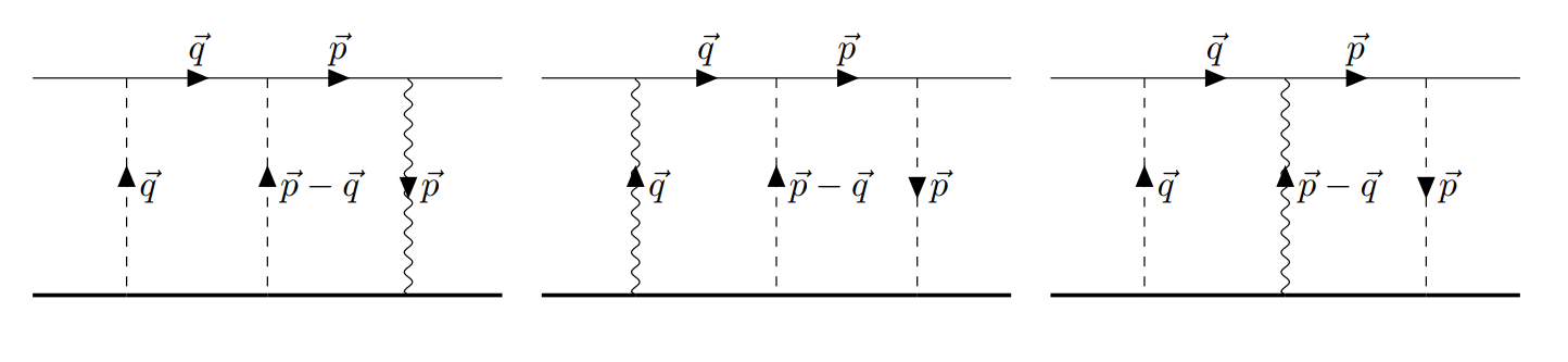
Figure 1: Three diagrams representing contributions to the high-energy part $\delta E_{H}$. Wavy lines represent magnetic photons carrying potential (46), and dashed lines are electric photons carrying potential (37).

$$\delta E_{H}= \delta E_{H1}+\delta E_{H2}+\delta E_{H3}$$ (45)

$$\delta E_{H1}= \psi^{2}(0)\int\frac{d^{d}p}{(2\,\pi)^{d}}\,\int\frac{d^{d}q}{(2\,\pi)^{d}}\bra{\bar{t}}e\vec{\gamma}\cdot\vec{A}(-\vec{p})$$

$$\times\frac{1}{\not{p}-1}\gamma^{0}V(\vec{p}-\vec{q})\frac{1}{\not{q}-1}\gamma^{0}V(\vec{q})\ket{t},$$

$$\delta E_{H2}= \psi^{2}(0)\int\frac{d^{d}p}{(2\,\pi)^{d}}\,\int\frac{d^{d}q}{(2\,\pi)^{d}}\bra{\bar{t}}\gamma^{0}V(-\vec{p})$$

$$\times\frac{1}{\not{p}-1}\gamma^{0}V(\vec{p}-\vec{q})\frac{1}{\not{q}-1}e\vec{\gamma}\cdot\vec{A}(\vec{q})\ket{t},$$

$$\delta E_{H3}= \psi^{2}(0)\int\frac{d^{d}p}{(2\,\pi)^{d}}\,\int\frac{d^{d}q}{(2\,\pi)^{d}}\bra{\bar{t}}\gamma^{0}V(-\vec{p})$$

$$\times\frac{1}{\not{p}-1}e\vec{\gamma}\cdot\vec{A}(\vec{p}-\vec{q})\frac{1}{\not{q}-1}\gamma^{0}V(\vec{q})\ket{t},$$

where $t=(1,\vec{0})$, $\not{p}=(1,\vec{p})^{\nu}\gamma_{\nu}$, and

$$A^{i}(q)=\frac{i\,Z\,e\,g_{p}}{4\,m_{p}}\sigma_{p}^{ik}\frac{q^{k}}{q^{2}}G_{M}(q^{2})\,.$$ (46)

After performing Dirac algebra, $\delta E_{H}$ can be expressed in the coordinate representation as

$$\delta E_{H} = \frac{8\psi^{2}(0)}{dm_{p}}(Z\alpha)^{3}g_{p}\braket{\vec{s}_{p}\cdot\vec{s}_{\mu}}_{\epsilon}$$ (47)

$$\times\int d^{d}r\left(2\pi\rho_{M}(r)[\mathcal{V}_{E}^{(2)}]^{2}+\mathcal{V}_{M}\mathcal{V}_{E}\mathcal{V}_{E}^{(2)}\right)\,,$$

where $d$-dimensional potentials $\mathcal{V}_{E}$ and $\mathcal{V}_{M}$ are defined in Appendix A. The first term under the integral sign is convergent due to the presence of $\rho_{M}$ and thus can be evaluated in three dimensions. The second term, however, contains a singularity $\sim 1/\epsilon$, which has to be separated out. This is achieved by splitting the domain of integration into $(0,\Lambda)$ and $(\Lambda,\infty)$. The integral over $(\Lambda,\infty)$ is evaluated by using the asymptotic form of the potentials in $d$ dimensions. The final result for the high-energy part is

$$\delta E_{H}=\frac{4}{d}(r_{p}Z\alpha)^{2}E_{F}\left[\frac{1}{4\epsilon}+\ln r_{pp}+\frac{1}{2}+\gamma\right]\,.$$ (48)

Here, $r_{pp}$ is the effective radius defined by

$$\ln\frac{r_{pp}}{r_{p}}= \frac{1}{G_{E}^{\prime}(0)}\int_{0}^{\infty}dr\ln\frac{r}{r_{p}}\frac{d}{dr}r^{3}\bigg{\{}2\pi\rho_{M}(r)[V_{E}^{(2)}]^{2}$$

$$+V_{M}V_{E}V_{E}^{(2)}+\frac{1}{r^{2}}\left(\frac{r}{2}-\frac{G_{E}^{\prime}(0)}{r}\right)\bigg{\}},$$ (49)

where $V_{E(M)}$ are three-dimensional versions of potentials $\mathcal{V}_{E(M)}$, which depend on electric and magnetic formfactors, and are presented in Appendix A.

The final result for the elastic three-photon exchange correction, $\delta^{(2)}E_{\text{fns}}=\delta E_{L}+\delta E_{H}$, with $m$ restored from dimensional analysis, is

$$\delta^{(2)}E_{\text{fns}}= \frac{4}{3}E_{F}(mr_{p}Z\alpha)^{2}\bigg{[}-\frac{1}{n}+2\gamma-\ln\frac{n}{2}+\Psi(n)$$

$$+\ln(mr_{pp}Z\alpha)+\frac{r_{m}^{2}}{4r_{p}^{2}n^{2}}\bigg{]}\,.$$ (50)

This expression is valid for any nucleus, both for muonic and electronic atoms.

For the dipole parametrization of the nuclear formfactors

$$G_{E}(q)=G_{M}(q)=\frac{1}{(1+q^{2}/\Lambda^{2})^{2}}\,,$$ (51)

one easily obtains the following results

$$r_{m}=r_{p}\,,\ \ r_{Z}/r_{p}=\frac{35}{16\sqrt{3}}\,,\ \ r_{pp}/r_{p}=5.274\,565\ldots\,,$$ (52)

which are independent of parameter $\Lambda$ and thus valid for any nucleus. Numerical values of the elastic $(Z\alpha)^{2}\,E_{F}$ correction for the $1S$ and $2S$ states of muonic hydrogen are

$$\delta^{(2)}E_{\text{fns}}(\mu{\rm H})=\left\{\begin{array}[]{ll}$-0.0093\text{\,}\mathrm{meV}$\,,&\mbox{\rm for the $1S$ state}\,,\\ $-0.000\,96\text{\,}\mathrm{meV}$\,,&\mbox{\rm for the $2S$ state}\,.\end{array}\right.$$ (55)

The above result for the $2S$ state deviates from the value of $-0.00065$ meV calculated by Indelicato Indelicato (2013) and quoted by Antognini et al. Antognini et al. (2013a) (entry h21 in Table III of that work). One of possible reasons could be the inclusion of the reduced mass in Indelicato’s calculation, while our result is obtained in the nonrecoil limit. We claim that the recoil effect on this relativistic correction cannot be accounted for in terms of the reduced mass. Our analytic result is verified by a numerical calculation in the following subsection.

III.3 Numerical verification

The analytical expression (50) for the fns correction of order $(Z\alpha)^{2}E_{F}$ has been verified by comparison with the numerical evaluation of the fns correction to all orders in $Z\alpha$. Specifically, the numerical all-order fns correction was obtained by evaluating the expectation value of the Fermi-Breit operator $H_{\mu}$ with solutions of the Dirac equation with an extended nucleus and subtracting the point-nucleus result. The (extended-nucleus) Fermi-Breit operator is

$$H_{\mu}=\frac{|e|}{4\pi}\frac{\bm{\alpha}\cdot[\bm{\mu}\times\bm{r}]}{r^{3}}\,F(r)\,,$$ (56)

where $\bm{\mu}$ is the nuclear magnetic moment operator, $\bm{\alpha}$ is the vector of Dirac matrices, and $F(r)$ describes the radial distribution of the magnetic moment, $F(r)\approx 1$ outside of the nucleus. For the dipole parametrization (51), the distribution function is given by

$$F(r)=1-e^{-\lambda r}\Big{(}1+\lambda r+\frac{1}{2}(\lambda r)^{2}\Big{)}\,,$$ (57)

where $\lambda=2\sqrt{3}/r_{m}$.

We define the relativistic fns correction that contains orders $(Z\alpha)^{2}E_{F}$ and higher by subtracting the Zemach contribution from the numerical fns correction,

$$\delta^{(2+)}E_{\text{fns}}=E_{\text{fns,num}}-\delta E_{\text{Zem}}\,.$$ (58)

Results for the relativistic fns correction are presented in Fig. 2, which demonstrates agreement between the numerical and analytical approaches for $Z=0$. The difference between the numerical and analytical results scales linearly with $Z$, representing the contribution of orders $(Z\alpha)^{3}E_{F}$ and higher.

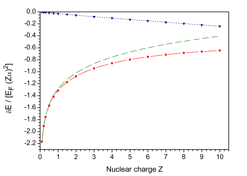
Figure 2: Numerical and analytical results for the fns correction normalized by the factor of $E_{F}(Z\alpha)^{2}$, for the $1S$ state of muonic hydrogen-like ions with the nuclear root-mean-square radius 1 fm, as a function of nuclear charge $Z$. Solid line and dots (red) represent numerical results (58); dashed line (green) shows analytical results (50); dotted line and triangles (blue) show the difference.

IV Three-photon exchange nuclear structure correction

In this section we address the inelastic three-photon exchange nuclear-structure correction $\sim\!(Z\,\alpha)^{2}\,E_{F}$ to the hyperfine splitting, which has not been studied in the literature so far. We will perform an approximate treatment of this correction and evaluate the largest contribution, namely that due to the electric dipole polarizability. Furthermore, we will demonstrate partial cancellations occurring between the elastic and inelastic parts for the case of muonic deuterium, $\mu$D.

The nuclear-structure correction $\delta^{(2)}E_{\rm nucl}$ can be represented as a sum of several contributions,

$$\delta^{(2)}E_{\rm nucl}=\delta E_{\text{DP}}+\delta E_{L}(D)+\delta E_{H}(p)+\delta E_{H}(pn)$$ (59)

where $\delta E_{\text{DP}}$ is the low-energy dipole polarizability contribution, $\delta E_{L}(D)$ is the elastic low-energy part, and $\delta E_{H}(p)$ and $\delta E_{H}(pn)$ are the high-energy corrections.

It is convenient to introduce the common factor

$$\mathcal{E}=\frac{4\pi\,\alpha}{3m_{p}}\,\psi^{2}(0)\,,$$ (60)

which will frequently appear in formulas below.

IV.1 Elastic low-energy contribution

The elastic low-energy part $\delta E_{L}(D)$ can be obtained from Eq. (44) by replacing the proton charge $r_{p}$ and magnetic $r_{m}$ radii with their deuteron counterparts $r_{d}$ and $r_{md}$, because at low energies muon sees the nucleon as a whole. The resulting expression is

$$\delta E_{L}(D)= \frac{4}{d}(r_{d}\alpha)^{2}\mathcal{E}\bigg{[}-\frac{1}{4\epsilon}-\frac{1}{n}-\frac{1}{2}+\gamma-\ln\frac{n}{2}+$$

$$\Psi(n)+\ln\alpha+\frac{r_{md}^{2}}{4r_{d}^{2}n^{2}}\bigg{]}\,g_{d}\,\Braket{\vec{s}_{d}\cdot\vec{s}_{\mu}}_{\epsilon},$$ (61)

where $\Braket{\vec{s}_{d}\cdot\vec{s}_{\mu}}_{\epsilon}$ is defined in Eq. (84).

IV.2 Polarizability contribution

We derive here the leading dipole polarizability correction $\delta E_{\text{DP}}$ and represent it as a sum of two terms

$$\delta E_{\text{DP}}=\delta E_{\text{DP1}}+\delta E_{\text{DP2}}$$ (62)

The first one $\delta E_{\text{DP1}}$ is obtained by taking the second-order matrix element with dipole interaction in the nonrelativistic approximation and perturbing it with the magnetic dipole-dipole interaction $H_{\text{hfs}}$. The result is

$$\delta E_{\text{DP1}}= \ \alpha^{2}\delta_{\text{hfs}}\biggl{\langle}\psi\phi_{N}\bigg{|}\vec{R}\cdot\vec{\nabla}\left[\frac{1}{r}\right]_{\epsilon}$$ (63)

$$\ \times\frac{1}{E_{N}+E_{0}-H_{N}-H_{0}}\vec{R}\cdot\vec{\nabla}\left[\frac{1}{r}\right]_{\epsilon}\bigg{|}\psi\phi_{N}\biggr{\rangle}\,.$$

Here, $\vec{R}$ is the proton position with respect to the deuteron mass center and $\delta_{\text{hfs}}$ denotes the first-order perturbation due to the hyperfine interaction $H_{\text{hfs}}$ which is an analog of $H_{\rm hfs}$ in Eq. (40) for the deuterium

$$H_{\text{hfs}}=\frac{4\pi\alpha}{dm_{p}}\delta^{(d)}(\vec{r})\,g_{d}(\vec{s}_{d}\cdot\vec{s}_{\mu})_{\epsilon},$$ (64)

where $H_{N}$ is the nuclear Hamiltonian and $H_{0}$ is the nonrelativistic muon Hamiltonian defined in Eq. (39). The perturbative treatment of $H_{\text{hfs}}$ means that the polarizability correction is expressed as a sum of two terms, originating from perturbations of the denominator and the wave function. However, the first term vanishes and $\delta E_{\rm DP1}$ becomes

$$\delta E_{\text{DP1}} = 2\alpha^{2}\bigg{\langle}\psi\phi_{N}\bigg{\rvert}\vec{R}\cdot\vec{\nabla}\left[\frac{1}{r}\right]_{\epsilon}\frac{1}{E_{0}+E_{N}-H_{0}-H_{N}}\vec{R}\cdot\vec{\nabla}\left[\frac{1}{r}\right]_{\epsilon}\frac{1}{(E_{0}-H_{0})^{\prime}}H_{\text{hfs}}\bigg{\lvert}\psi\phi_{N}\bigg{\rangle}\,,$$ (65)

Because we are interested in the leading correction only, we neglect the $D$-wave in the ground deuteron state and neglect the Coulomb corrections, so

$$\delta E_{\text{DP1}} = \frac{12}{d^{2}}\alpha^{2}\mathcal{E}\sum_{\Lambda}\bra{\phi_{N}}\vec{R}\ket{\Lambda}\bra{\Lambda}\vec{R}\ket{\phi_{N}}g_{d}\braket{\vec{s}_{d}\cdot\vec{s}_{\mu}}_{\epsilon}\int\frac{d^{d}p}{(2\pi)^{d}}\frac{d^{d}q}{(2\pi)^{d}}\frac{4\pi}{p^{2}}\frac{4\pi}{q^{2}}\frac{\vec{p}\cdot\vec{q}}{(\vec{p}-\vec{q})^{2}}\frac{2}{p^{2}+2\Lambda}.$$ (66)

After integration we obtain the following expression for the polarizability correction

$$\delta E_{\text{DP1}}=\frac{4}{d}(r_{s}\alpha)^{2}\mathcal{E}\bigg{(}\frac{1}{4\epsilon}+\frac{2}{3}-\frac{1}{2}\ln 2\bar{E}\bigg{)}\Braket{g_{d}\vec{s}_{d}\cdot\vec{s}_{\mu}}_{\epsilon}\\ \,,$$ (67)

where $\bar{E}$ is the mean excitation energy defined by

$$\ln\frac{\bar{E}}{m}=\frac{1}{r_{s}^{2}}\Braket{\phi_{N}}{\vec{R}\ln\biggl{[}\frac{(H_{N}-E_{N})}{m}\biggr{]}\vec{R}}{\phi_{N}}\,.$$ (68)

and $r_{s}$ is the deuteron structure radius

$$r_{s}=\sqrt{\Braket{R^{2}}}\,.$$ (69)

The mean excitation energy (68) was calculated in Ref. Pachucki et al. (2018) using the AV18 potential wiringa:95 , with the result

$$\bar{E}=$7.37(7)\text{\,}\mathrm{MeV}$.$$ (70)

The pion-less EFT in the next-to-leading order Friar (2013) reproduces this result with $2\text{\,}\mathrm{\char 37\relax}$ accuracy.

The second dipole polarizability contribution $\delta E_{\rm DP2}$ is the Coulomb distortion correction to the leading two-photon exchange contribution $\delta E_{\rm pol1}$ in Eq. (24). We derive it by considering the nonrelativistic formula for the second order correction to energy that comes from the electric dipole interaction and the magnetic quadrupole term in Eq. (22)

$$\delta E_{\rm DP2}= \ 4\pi\alpha^{2}\,\frac{g_{p}-g_{n}}{dm_{p}}\Braket{\vec{s}_{d}\cdot\vec{s}_{\mu}}_{\epsilon}\delta_{C}\biggl{\langle}\psi\phi_{N}|\vec{R}\cdot\vec{\nabla}\left[\frac{1}{r}\right]_{\epsilon}\frac{1}{H_{0}+H_{N}-E_{0}-E_{N}}\vec{R}\cdot\vec{\nabla}\,\delta(\vec{r})|\psi\phi_{N}\biggr{\rangle},$$ (71)

where $\delta_{C}$ denotes the Coulomb correction, namely that beyond $E_{\rm pol1}$ in Eq. (24). This Coulomb correction is the forward scattering three-photon exchange amplitude, which takes the following form in the momentum representation

$$\delta E_{\rm DP2} =\frac{3\alpha^{2}}{d}\frac{g_{p}-g_{n}}{g_{d}}E_{F}\sum_{\Lambda^{\prime}}\braket{\phi_{N}}{R^{k}}{\Lambda}\braket{\Lambda}{R^{i}}{\phi_{N}}\int\frac{d^{d}p}{(2\pi)^{d}}\frac{d^{d}q}{(2\pi)^{d}}\frac{4\,\pi\,p^{k}}{p^{2}}\frac{4\,\pi\,q^{i}}{\frac{q^{2}}{2}+\Lambda}\biggl{[}\frac{1}{\frac{p^{2}}{2}+\Lambda}\frac{1}{\left\lvert\vec{p}-\vec{q}\right\rvert^{2}}+\frac{2}{\left\lvert\vec{p}-\vec{q}\,\right\rvert^{4}}\biggr{]}.$$ (72)

After integration we obtain for $\delta E_{\rm DP2}$

$$\delta E_{\rm DP2}=\frac{4}{3}(\alpha\,r_{s})^{2}\frac{g_{p}-g_{n}}{g_{d}}E_{F}\left(\frac{3}{4}-\ln 2\right)$$ (73)

Its value is heavily suppressed by the numerical factor in the parentheses.

IV.3 High-energy contribution $\delta E_{H}(pn)$

When muon momentum is of the order of the inverse of internucleon distance, the muon sees different positions of the proton and the neutron inside the nucleus, and effectively one can discern which photon interacts with which nucleon in the three-photon exchange. Because one can neglect the nuclear excitation energy in comparison to the muon kinetic energy, the high-energy contribution can be represented as an expectation value of the effective interaction potential,

$$\delta E_{H}(pn)=\langle\phi_{N}|\delta V_{H}|\phi_{N}\rangle\,,$$ (74)

where

$$\delta V_{H} =\psi^{2}(0)\,\int\frac{d^{d}p}{(2\,\pi)^{d}}\,\int\frac{d^{d}q}{(2\,\pi)^{d}}\bigl{[}\delta V_{H1}+\delta V_{H2}+\delta V_{H2}\bigr{]}\,,$$ (75)

and

$$\delta V_{H1} =\bra{\bar{t}}e\vec{\gamma}\cdot\vec{A}_{a}(-\vec{p})e^{i\vec{p}\cdot\vec{R}_{a}}\frac{1}{\not{p}-1}\gamma^{0}V_{b}(\vec{p}-\vec{q})e^{i(\vec{q}-\vec{p})\cdot\vec{R}_{b}}\frac{1}{\not{q}-1}\gamma^{0}e^{-i\vec{q}\cdot\vec{R}_{c}}V_{c}(\vec{q})\ket{t},$$

$$\delta V_{H2} =\bra{\bar{t}}\gamma^{0}V_{c}(-\vec{p})e^{i\vec{p}\cdot\vec{R}_{c}}\frac{1}{\not{p}-1}\gamma^{0}V_{b}(\vec{p}-\vec{q})e^{i(\vec{q}-\vec{p})\cdot\vec{R}_{b}}\frac{1}{\not{q}-1}e^{-i\vec{q}\cdot\vec{R}_{a}}e\vec{\gamma}\cdot\vec{A}_{a}(\vec{q})\ket{t},$$

$$\delta V_{H3} =\bra{\bar{t}}\gamma^{0}V_{b}(-\vec{p})e^{i\vec{p}\cdot\vec{R}_{b}}\frac{1}{\not{p}-1}e\vec{\gamma}\cdot\vec{A}_{a}(\vec{p}-\vec{q})e^{i(\vec{q}-\vec{p})\cdot\vec{R}_{a}}\frac{1}{\not{q}-1}\gamma^{0}e^{-i\vec{q}\cdot\vec{R}_{c}}V_{c}(\vec{q})\ket{t}.$$

Indices $(a,b,c)\in\{p,n\}$ discern whether the interacting nucleon is the proton or the neutron. We neglect all the contributions where the electric photon interacts with the neutron ($b=c=p$) and thus are left with two cases. We first consider the case when the magnetic photon hits the neutron ($a=n$). This gives the following correction

$$\delta E_{H}(pn)=\frac{8\psi^{2}(0)}{dm_{p}}\alpha^{3}g_{n}\braket{\vec{s}_{n}\cdot\vec{s}_{\mu}}_{\epsilon}$$ (76)

$$\times\bigg{\langle}\phi_{N}\bigg{\rvert}\int d^{d}r\bigg{(}2\pi\rho_{M}(\vec{r}+2\,\vec{R})\,[\mathcal{V}_{E}^{(2)}]^{2}$$

$$+\mathcal{V}_{M}(\vec{r}+2\,\vec{R})\,\mathcal{V}_{E}\mathcal{V}_{E}^{(2)}\bigg{)}\bigg{\lvert}\phi_{N}\bigg{\rangle}\,,$$

which is almost the same as Eq. (47), but has magnetic terms shifted by the proton-neutron distance. All the potentials in Eq. (76) are functions of $r$, unless explicitly written and magnetic potentials refer to the neutron formfactor, while electric ones to the proton one, both through definitions (86). The treatment of Eq. (76) follows the same pattern as that of Eq. (47). The only difference is that magnetic factors are shifted by $2\,\vec{R}$, which leads to additional terms. The result is

$$\delta E_{H}(pn) =\frac{4}{d}(r_{p}\alpha)^{2}\mathcal{E}g_{n}\Braket{\vec{s}_{n}\cdot\vec{s}_{\mu}}_{\epsilon}$$

$$\times\bigg{(}\frac{1}{4\epsilon}+\gamma-\frac{1}{2}+\frac{3r_{pn}^{2}+2r_{s}^{2}}{r_{p}^{2}}+\ln 2r_{l}\bigg{)},$$ (77)

where $r_{l}$ is defined as

$$\ln\left(2mr_{l}\right)=\braket{\phi_{N}}{\ln\left(2mR\right)}{\phi_{N}}$$ (78)

and its value can be found in Table 1. The effective proton-neutron radius $r_{pn}$ in Eq. (IV.3) is defined as

$$2\pi{r_{pn}^{2}}=\bigg{\langle}\phi_{N}\bigg{\rvert}\int d^{3}r\Bigg{(}2\pi\rho_{M}(\vec{r}+2\,\vec{R})[V_{E}^{(2)}]^{2}$$ (79)

$$+V_{M}(\vec{r}+2\,\vec{R})\,V_{E}\,V_{E}^{(2)}+\frac{1}{\lvert\vec{r}+2\,\vec{R}\rvert}\,\bigg{(}\frac{1}{2}-\frac{G_{E}^{\prime}(0)}{r^{2}}\bigg{)}\Bigg{)}\bigg{\lvert}\phi_{N}\bigg{\rangle}.$$

where $\rho_{M}$ and $V_{M}$ correspond to the neutron, while $G_{E}$ and $V_{E}$ correspond to the proton. It is worth noting that in the point-nucleon limit the proton-neutron effective radius $r_{pn}$, given by Eq. (79), is equal to the deuteron structure radius ($r_{pn}\rightarrow r_{s}$).

IV.4 High-energy contribution $\delta E_{H}(p)$

In the case when all three photons interact with the proton, one should use the complete four-vector current, as in the two-photon case. We are not able to perform such a calculation at present, and thus we assume that the dominating contribution comes from the elastic part in the nonrecoil limit,

$$\delta E_{H}(p)= \frac{4}{d}(r_{p}\alpha)^{2}\mathcal{E}\left[\frac{1}{4\epsilon}+\ln r_{pp}+\frac{1}{2}+\gamma\right]\!g_{p}\Braket{\vec{s}_{p}\cdot\vec{s}_{\mu}}_{\epsilon}\,.$$ (80)

IV.5 Total three-photon exchange correction

Summing all contributions in Eq. (59) and restoring $m$’s from dimensional analysis, we obtain the three-photon nuclear-structure correction of order $(Z\,\alpha)^{2}\,E_{F}$ for $\mu$D,

$$\delta^{(2)}E_{\rm nucl}= \frac{4}{3}(m\alpha)^{2}E_{F}\bigg{[}r_{pn}^{2}\frac{3g_{n}}{2g_{d}}+r_{md}^{2}\frac{1}{4n^{2}}+r_{s}^{2}\bigg{(}\frac{g_{n}}{g_{d}}-\gamma$$

$$+\frac{g_{p}-g_{n}}{g_{d}}\left(\frac{3}{4}-\ln 2\right)+\frac{1}{6}-\frac{1}{2}\ln\frac{2\bar{E}}{m}\bigg{)}$$

$$+r_{d}^{2}\left(2\gamma-\frac{1}{n}-\ln\frac{n}{2}+\Psi(n)+\ln\alpha\right)$$

$$+r_{p}^{2}\bigg{(}g_{p}\ln(mr_{pp})+g_{n}\ln(2mr_{l})-g_{n}\bigg{)}\frac{1}{2g_{d}}\bigg{]}\,.$$

In deriving this final formula we made use of an approximate identity $\braket{g_{d}\vec{s}_{d}}\approx\braket{g_{p}\vec{s}_{p}+g_{n}\vec{s}_{n}}/$ to cancel out the $\epsilon$ singularity and $\braket{\vec{s}_{p}}=\braket{\vec{s}_{n}}=\braket{\vec{s}_{d}}/2$ for further simplifications. Numerical values for all parameters in the final formula are listed in Table 1.

Table 1: Effective radii and $g$-factors for the three-photon nuclear-structure correction for $\mu$D, given by Eq. (IV.5). Proton-neutron radius $r_{pn}$ is taken in the point-nucleon limit ($r_{pn}=r_{s}$) and $r_{l}$ is obtained with the AV18 potential wiringa:95

Variable	Value	Units	Source
$r_{p}$	$0.84087(39)$	fm	Ref. Antognini et al. (2013b)
$r_{d}$	$2.1256(8)$	fm	Ref. Pohl et al. (2017)
$r_{s}$	$1.954661(79)$	fm	Ref. Pachucki et al. (2018)
$r_{md}$	$2.312(10)$	fm	Ref. Afanasev et al. (1998)
$r_{pp}$	$4.435$	fm	Eq. (III.2)
$r_{pn}$	$1.955$	fm	Eq. (79)
$r_{p\rm Z}$	$0.883(19)$	fm	Ref. toamalak_arxiv_18
$r_{n\rm Z}$	$0.06(1)$	fm	Ref. tomalak
$r_{l}$	$1.339$	fm	Eq. (78)
$g_{p}$	$5.585694702(17)$		Ref. Mohr et al. (2016)
$g_{d}$	$0.8574382311(48)$		Ref. Mohr et al. (2016)
$g_{n}$	$-3.82608545(90)$		Ref. Mohr et al. (2016)

Our final results for the three-photon exchange deuteron structure correction $\delta^{(2)}E_{\rm nucl}$ are presented in Table 2. We assume a $25\text{\,}\mathrm{\char 37\relax}$ uncertainty of these results, due to neglect of the polarizability corrections beyond the electric dipole contribution and of the unknown inelastic proton contribution, although we must admit that we can not well justify this uncertainty estimate.

Our results for the three-photon exchange structure correction disagree with corresponding formulas obtained by Faustov et al. Faustov et al. (2014) (given by Eqs. (55), (58), and (59) of that work). The reason for this disagreement is two-fold. First, Faustov et al. considered only the low-energy part of the nuclear-structure correction, omitting completely the high-energy part. Second, the term proportional to the deuteron magnetic radius $r_{md}$ in their calculation contains an additional factor of $1/n^{3}$, due to a mistake in evaluation of the matrix element presented in Eq. (89).

V Summary

A summary of all known nuclear-structure contributions to the hyperfine splitting of the $1S$ and $2S$ states in $\mu$D is presented in Table 2.

Table 2: Nuclear structure corrections for hyperfine splitting of the $1S$ and $2S$ states of muonic deuterium, in meV. Numerical results are obtained with the AV18 potential wiringa:95 .

Correction	$1S$	$2S$	Source
$\delta E_{\rm pol1}$	$-1.1007$	$-0.1376$	Eq. (24)
$\delta E_{\rm pol2}$	$-0.0823$	$-0.0103$	Eq. (27)
$\delta E_{\rm pol3}$	$0.1513$	$0.0189$	Eq. (28)
$\delta E_{\rm pol4}$	$-0.1979$	$-0.0283$	Eq. (32)
$\delta E_{\rm pol5}$	$-0.0327$	$-0.0041$	Eq. (34)
$\delta E_{\rm pol}$	$-1.2623(631)$	$-0.1578(79)$	Eq. (35)
$\delta E_{\rm 1nucl}$	$-0.9450(224)$	$-0.1181(28)$	Eq. (17)
$\delta E_{\rm Low}$	$2.566$	$0.3208$	Eq. (16)
$\delta^{(1)}E_{\rm nucl}$	$0.3587(670)$	$0.0448(84)$	Eq. (14)
$\delta^{(2)}E_{\rm nucl}$	$-0.0547(137)$	$-0.0065(16)$	Eq. (IV.5)
$\delta E_{\rm nucl,theo}$	$0.304(68)$	$0.0383(86)$	Eq. (10)
$\delta E_{\rm nucl,exp}$		$0.0966(73)$	Eq. (9)
difference		$0.0583(113)$

We find that the total theoretical result for the deuteron structure correction for the $2S$ state differs from the experimental value by about $5\,\sigma$. A possible reason for this discrepancy might be our insufficient knowledge of the spin-dependent coupling of nucleus to the electromagnetic field, in particular the unknown corrections to the nonrelativistic current in Eq. (II). Another possible reason could be a mistake in calculations of QED effects for the point nucleus, although it looks much less probable since these calculations were performed independently by two groups borie:14 ; Faustov et al. (2014).

Summarizing, in the present work we have calculated the two- and three-photon exchange nuclear structure corrections to the hyperfine splitting of the $nS$ states in $\mu$D. The obtained results disagree with the previous theoretical calculation Faustov et al. (2014) and with the experimental result pohl:16 .

Appendix A Dimensional regularization

In order to extend spin $\frac{1}{2}$ into $d$ dimensions, we define antisymmetric tensor

$$\sigma^{ij}=\frac{i}{2}[\gamma^{i},\gamma^{j}]\,,$$ (82)

that in the three-dimensional limit simplifies to

$$\sigma^{ij}\overset{d\rightarrow 3}{=}2\varepsilon^{ijk}s^{k}.$$ (83)

Additionally, for the deuteron we define $\sigma_{d}^{ij}=\sigma_{p}^{ij}+\sigma_{n}^{ij}$ and use the following convenient notation

$$(\vec{s}_{a}\cdot\vec{s}_{b})_{\epsilon} =\frac{1}{8}\sigma_{a}^{ij}\sigma_{b}^{ij}$$ (84)

Throughout our calculations we extensively used the following result for the general $d$-dimensional integral,

$$\int\frac{d^{d}p}{(2\pi)^{d}}\frac{4\pi}{p^{n}}e^{i\vec{p}\cdot\vec{r}}=2^{2-n}\pi^{1-d/2}\frac{\Gamma\left(\frac{d-n}{2}\right)}{\Gamma\left(\frac{n}{2}\right)}r^{n-d}\,.$$ (85)

Two special cases are of particular importance (with $d=3-2\epsilon$):

$$\mathcal{V}(r) =\int\frac{d^{d}p}{(2\pi)^{d}}\frac{4\pi}{p^{2}}e^{i\vec{p}\cdot\vec{r}} =\pi^{\epsilon-1/2}\Gamma(1/2-\epsilon)\frac{1}{r^{1-2\epsilon}},$$

$$\mathcal{V}^{(2)}(r) =\int\frac{d^{d}p}{(2\pi)^{d}}\frac{4\pi}{p^{4}}e^{i\vec{p}\cdot\vec{r}} =\frac{1}{4}\pi^{\epsilon-1/2}\Gamma(-1/2-\epsilon)r^{1+2\epsilon}.$$

We define also the associated potentials:

$$\mathcal{V}_{X} = 4\pi\int\frac{d^{d}p}{(2\pi)^{d}}\frac{G_{X}(p^{2})}{p^{2}}e^{i\vec{p}\cdot\vec{r}},$$

$$\mathcal{V}_{X}^{(2)} = 4\pi\int\frac{d^{d}p}{(2\pi)^{d}}\frac{G_{X}(p^{2})}{p^{4}}e^{i\vec{p}\cdot\vec{r}},$$ (86)

where $X\in\{E,M\}$. Asymptotic forms of these potentials at $r\rightarrow\infty$ are:

$$\mathcal{V}_{X} \rightarrow \mathcal{V}+\text{local terms},$$

$$\mathcal{V}_{X}^{(2)} \rightarrow \mathcal{V}^{(2)}+G_{X}^{\prime}(0)\mathcal{V}+\text{local terms}\,.$$

The corresponding three-dimensional potentials are

$$V_{X}= \ 4\pi\int\frac{d^{3}p}{(2\pi)^{3}}\frac{G_{X}(p^{2})}{p^{2}}e^{i\vec{p}\cdot\vec{r}},$$

$$V_{X}^{(2)}= \ 4\pi\int\frac{d^{3}p}{(2\pi)^{3}}\frac{[G_{X}(p^{2})-1]}{p^{4}}e^{i\vec{p}\cdot\vec{r}},$$ (87)

with the asymptotic form

$$V_{X} \rightarrow \frac{1}{r}+\text{local terms},$$

$$V_{X}^{(2)} \rightarrow -\frac{r}{2}+\frac{G_{X}^{\prime}(0)}{r}+\text{local terms}.$$ (88)

Furthermore, we point out that in the framework of dimensional regularization the following matrix element vanishes

$$\Braket{\vec{p}~{}\delta^{(d)}(\vec{r})~{}\vec{p}}=0.$$ (89)

References

• (1) J.J. Krauth, M. Diepold, B. Franke, A. Antognini, F. Kottmann, and R. Pohl, Ann. Phys. 366, 168 (2016).
• (2) E. Borie, arXiv:1103.1772-v7 [physic.atom-ph] (2014).
• Faustov et al. (2014) R. N. Faustov, A. P. Martynenko, G. A. Martynenko, and V. V. Sorokin, Phys. Rev. A 90, 012520 (2014).
• (4) R. Pohl et al., Science 353, 669 (2016).
• Zemach (1956) A. C. Zemach, Phys. Rev. 104, 1771 (1956).
• (6) J. Friar and I. Sick, Phys. Lett. B, 579, 285 (2004)
• Tomalak (2017) O. Tomalak, Eur. Phys. J. C 77, 858 (2017).
• Carlson et al. (2008) C. E. Carlson, V. Nazaryan, and K. Griffioen, Phys. Rev. A 78, 022517 (2008).
• Carlson et al. (2011) C. E. Carlson, V. Nazaryan, and K. Griffioen, Phys. Rev. A 83, 042509 (2011).
• Tomalak (2018) O. Tomalak, Eur. Phys. J. A 54, 3 (2018).
• Low (1950) F. Low, Phys. Rev. 77, 361 (1950).
• (12) R. B. Wiringa, V. G. J. Stoks, and R. Schiavilla, Phys. Rev. C 51, 38 (1995).
• Friar and Payne (2005a) J. Friar and G. Payne, Phys. Lett. B 618, 68 (2005a).
• Friar and Payne (2005b) J. L. Friar and G. L. Payne, Phys. Rev. C 72, 014002 (2005b).
• (15) O. Tomalak, arXiv:1808.09204 [hep-ph].
• (16) O. Tomalak, arXiv:1812.03884 [hep-ph].
• Khriplovich and Milstein (2004) I. B. Khriplovich and A. I. Milstein, JETP 98, 181 (2004).
• Pachucki (2007) K. Pachucki, Phys. Rev. A 76, 022508 (2007).
• Pachucki et al. (2018) K. Pachucki, V. Patkóš, and V. A. Yerokhin, Phys. Rev. A 97, 062511 (2018).
• Indelicato (2013) P. Indelicato, Phys. Rev. A 87, 022501 (2013).
• Antognini et al. (2013a) A. Antognini, F. Kottmann, F. Biraben, P. Indelicato, F. Nez, and R. Pohl, Ann. Phys. 331, 127 (2013a).
• Friar (2013) J. L. Friar, Phys. Rev. C 88, 034003 (2013).
• Antognini et al. (2013b) A. Antognini, F. Nez, K. Schuhmann, F. D. Amaro, F. Biraben, J. M. R. Cardoso, D. S. Covita, A. Dax, S. Dhawan, M. Diepold, et al., Science 339, 417 (2013b).
• Pohl et al. (2017) R. Pohl, F. Nez, T. Udem, A. Antognini, A. Beyer, H. Fleurbaey, A. Grinin, T. W. Hänsch, L. Julien, F. Kottmann, et al., Metrologia 54, L1 (2017).
• Afanasev et al. (1998) A. V. Afanasev, V. D. Afanasev, and S. V. Trubnikov, arXiv:nucl-th/9808047 (1998).
• Mohr et al. (2016) P. J. Mohr, D. B. Newell, and B. N. Taylor, Rev. Mod. Phys. 88, 035009 (2016).