MODELING NONLINEAR AUDIO EFFECTS WITH END-TO-END DEEP NEURAL NETWORKS

Abstract

In the context of music production, distortion effects are mainly used for aesthetic reasons and are usually applied to electric musical instruments. Most existing methods for nonlinear modeling are often either simplified or optimized to a very specific circuit. In this work, we investigate deep learning architectures for audio processing and we aim to find a general purpose end-to-end deep neural network to perform modeling of nonlinear audio effects. We show the network modeling various nonlinearities and we discuss the generalization capabilities among different instruments.

Index Terms—  audio effects modeling, virtual analog, deep learning, end-to-end, distortion.

1 Introduction

Audio effects modeling is the process of emulating an audio effect unit and often seeks to recreate the sound of an analog reference device [1]. Correspondingly, an audio effect unit is an analog or digital signal processing system that transforms certain characteristics of the sound source. These transformations can be linear or nonlinear, with memory or memoryless. Most common audio effects’ transformations are based on dynamics, such as compression; tone such as distortion; frequency such as equalization (EQ) or pitch shifters; and time such as artificial reverberation or chorus.

Nonlinear audio effects such as overdrive are widely used by musicians and sound engineers [2]. These type of effects are based on the alteration of the waveform which leads to amplitude and harmonic distortion. This transformation is achieved via the nonlinear behavior of certain components of the circuitry, which apply a waveshaping nonlinearity to the audio signal amplitude in order to add harmonic and inharmonic overtones. Thus, a waveshaping transformation consists in using a nonlinear function to distort the incoming waveform into a different shape, which depends on the amplitude of the incoming signal [3].

Since a nonlinear element cannot be characterized by its impulse response, frequency response or transfer function [1], digital emulation of nonlinear audio effects has been extensively researched [4]. Different methods have been proposed such as memoryless static waveshaping [5, 6], where system-identification methods are used in order to model the nonlinearity; dynamic nonlinear filters [7], where the waveshaping curve changes its shape as a function of system-state variables; analytical methods [8, 9], where the nonlinearity is linearized via Volterra series theory or black-box modeling such as Wiener and Hammerstein models [10, 11]; and circuit simulation techniques [12, 13, 14], where nonlinear filters are derived from the differential equations that describe the circuit. Recurrent neural networks have been explored as preliminary studies in [15, 16, 17], where the proposed models may require a more extensive evaluation.

In order to achieve optimal results, these methods are often either greatly simplified or highly optimized to a very specific circuit. Thus, without resorting to further complex analysis methods or prior knowledge about the circuit, it is difficult to generalize the methods among different audio effects. This lack of generalization is accentuated when we consider that each unit of audio effects is also composed of components other than the nonlinearity. These components also need to be modeled and often involve filtering before and after the waveshaping, as well as hysteresis or attack and release gates.

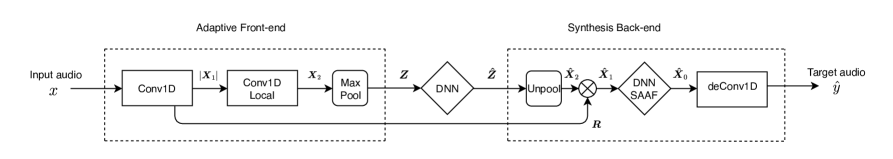
Fig. 1: Block diagram of the proposed model; adaptive front-end, synthesis back-end and latent-space DNN.

End-to-end learning corresponds to the integration of an entire problem as a single indivisible task that must be learned from end-to-end. The desired output is obtained from the input by learning directly from the data [18]. Deep learning architectures using this principle have experienced significant growth in music information retrieval [19, 20], since by learning directly from raw audio, the amount of required prior knowledge is reduced and the engineering effort is minimized [21].

End-to-end deep neural networks (DNN) for audio processing have been implemented in [22], where EQ modeling was achieved with convolutional neural networks (CNN). We build on this model in order to emulate much more complex transformations such as nonlinearities. To the best of our knowledge, prior to this work, deep learning architectures has not been successfully implemented to model nonlinear and linear audio effects.

We explore nonlinear emulation as a content-based transformation without explicitly obtaining the solution of the nonlinear system. We show the model performing nonlinear modeling for distortion, overdrive, amplifier emulation and combinations of linear and nonlinear audio effects.

2 Methods

2.1 Model

The model is entirely based on the time-domain and is divided into three parts: adaptive front-end, synthesis back-end and latent-space DNN. We build on the model from [22] and we incorporate a new layer into the synthesis back-end. The model is depicted in Fig. 1, and may seem similar to the nonlinear system measurement technique from [8], as it is based on a parallel combination of the cascade of input filters, memoryless nonlinearities, and output filters.

The adaptive front-end consist of a convolutional encoder. It contains two CNN layers, one pooling layer and one residual connection. The front-end performs time-domain convolutions with the raw audio in order to map it into a latent-space. It also generates a residual connection which facilitates the reconstruction of the waveform by the back-end.

The input layer has $128$ one-dimensional filters of size $64$ and is followed by the absolute value as nonlinear activation function. The second layer has $128$ filters of size $128$ and each filter is locally connected. This means we follow a filter bank architecture since each filter is only applied to its corresponding row in $|\boldsymbol{X}_{1}|$ and we also decrease significantly the number of trainable parameters. This layer is followed by the softplus nonlinearity.

From Fig. 1, $\boldsymbol{R}$ is the matrix of the residual connection, $\boldsymbol{X}_{1}$ is the feature map or frequency decomposition matrix after the input signal $x$ is convolved with the kernel matrix $\boldsymbol{W}_{1}$, and $\boldsymbol{X}_{2}$ is the second feature map obtained after the local convolution with $\boldsymbol{W}_{2}$, the kernel matrix of the second layer. The max-pooling layer is a moving window of size $16$, where positions of maximum values are stored and used by the back-end. Also, in the front-end, we include a batch normalization layer before the max-pooling operation.

The latent-space DNN contains two layers. Following the filter bank architecture, the first layer is based on locally connected dense layers of $64$ hidden units and the second layer consists of a fully connected layer of $64$ hidden units. Both of these layers are followed by the softplus function. Since $\boldsymbol{Z}$ corresponds to a latent representation of the input audio. The DNN modifies this matrix into a new latent representation $\boldsymbol{\hat{Z}}$ which is fed into the synthesis back-end. Thus, the front-end and latent-space DNN carry out the input filtering operations of the given nonlinear task.

The synthesis back-end inverts the operations carried out by the front-end and applies various dynamic nonlinearities to the modified frequency decomposition of the input audio signal $\hat{X}_{1}$. Accordingly, the back-end consists of an unpooling layer, a deep neural network with smooth adaptive activation functions (DNN-SAAF) and a single CNN layer.

DNN-SAAF: These consist of four fully connected dense layers of $128$, $64$, $64$ and $128$ hidden units respectively. All dense layers are followed by the softplus function with the exception of the last layer. Since we want the network to learn various nonlinear filters for each row of $\hat{X}_{1}$, we use locally connected Smooth Adaptive Activation Functions (SAAF) [23] as the nonlinearity for the last layer.

SAAFs consist of piecewise second order polynomials which can approximate any continuous function and are regularized under a Lipschitz constant to ensure smoothness. It has been shown that the performance of CNNs in regression tasks has improved when adaptive activation functions have been used [23], as well as their generalization capabilities and learning process timings [24, 25, 26].

We tested different types of adaptive activation functions, such as parametric hyperbolic tangent, parametric sigmoid and fifth order polynomials. Nevertheless, we found stability problems and non optimal results when modeling complex nonlinearities.

The back-end accomplishes the reconstruction of the target audio signal by the following steps. First, a discrete approximation $\boldsymbol{\hat{X}}_{2}$ is obtained by upsampling $\boldsymbol{Z}$ at the locations of the maximum values from the pooling operation. Then the approximation $\boldsymbol{\hat{X}}_{1}$ of matrix $\boldsymbol{X}_{1}$ is obtained through the element-wise multiplication of the residual $\boldsymbol{R}$ and $\boldsymbol{\hat{X}}_{2}$. In order to obtain $\hat{X}_{0}$, the nonlinear filters from DNN-SAAF are applied to $\hat{X}_{1}$. Finally, the last layer corresponds to the deconvolution operation, which can be implemented by transposing the first layer transform.

We train two types of models: model-1 without dropout layers within the dense layers of the latent-space DNN and DNN-SAAF, and model-2 with dropout layers among the hidden units of these layers. All convolutions are along the time dimension and all strides are of unit value. This means, during convolution, we move the filters one sample at a time. The models have approximately $600k$ trainable parameters, which represents a model that is not very large or difficult to train.

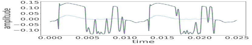
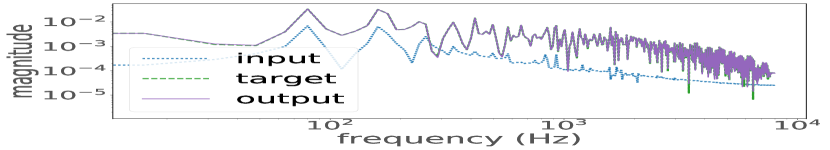
(a)

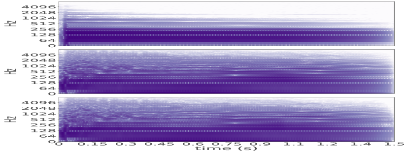
(b)

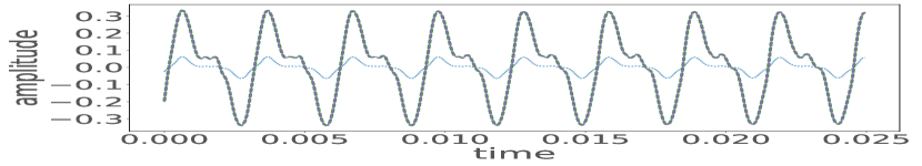
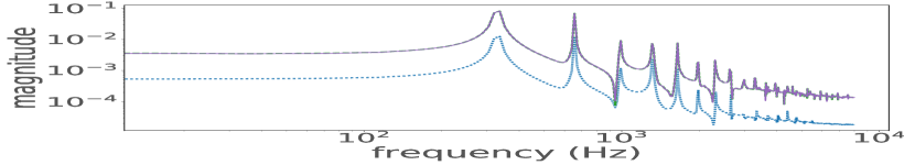
(c)

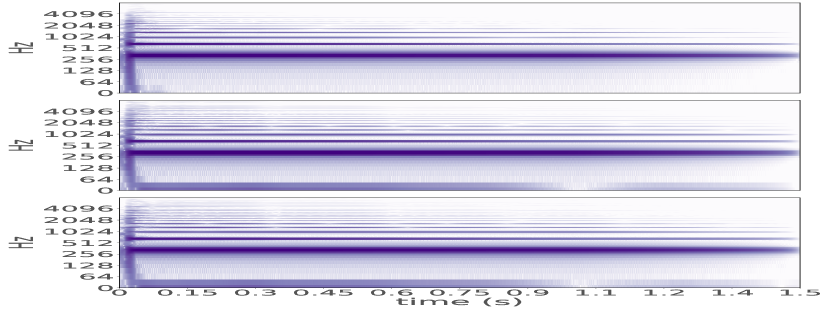
(d)

Fig. 2: Results with the test dataset for 2a-b) model-1 bass guitar distortion setting # 1, and 2c-d) model-2 electric guitar overdrive setting # 2. A segment of the input, target and output frames and their respective FFT magnitudes is shown. Also, from top to bottom: input, target and output spectrograms of the test samples; color intensity represents higher magnitude.

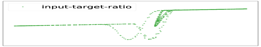
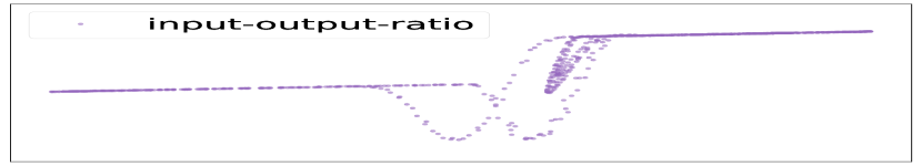
(a)

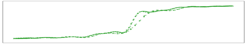
(b)

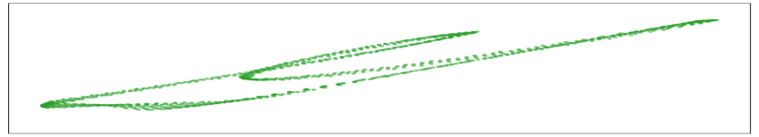
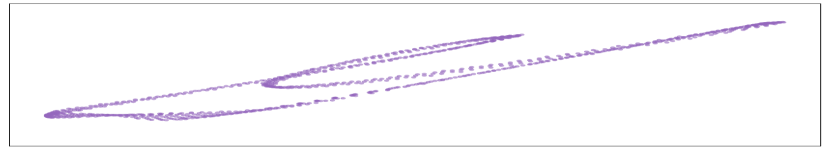
(c)

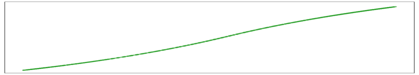
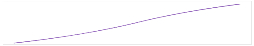
(d)

Fig. 3: Input-Target and Input-Output waveshaping curve for selected settings. 3a) model-1 bass guitar distortion task #1. 3b) model-1 electric guitar distortion setting #2. 3c) model-2 bass guitar overdrive setting #1. 3d) model-2 electric guitar overdrive setting #2. X-axis is input amplitude and Y-axis is target/output amplitude.

Based on end-to-end deep neural networks, we introduce a general purpose deep learning architecture for modeling nonlinear audio effects. Thus, for an arbitrary combination of linear and nonlinear memoryless audio effects, the model learns how to process the audio directly in order to match the target audio. Given a nonlinearity, consider $x$ and $y$ the raw and distorted audio signals respectively. In order to obtain a $\hat{y}$ that matches the target $y$, we train a deep neural network to modify $x$ based on the nonlinear task.

2.2 Training

The training of the model is performed in two steps. The first step is to train only the convolutional layers for an unsupervised learning task, while the second step is within a supervised learning framework for the entire network. During the first step only the weights of Conv1D and Conv1D-Local are optimized and both the raw audio $x$ and distorted audio $y$ are used as input and target functions.

Once the model is pretrained, the latent-space DNN and DNN-SAAF are incorporated into the model, and all the weights of the convolutional and dense layers are updated. The loss function to be minimized is the mean absolute error ($mae$) between the target and output waveforms. In both training procedures the input and target audio are sliced into frames of $1024$ samples with hop size of $64$ samples. The mini-batch was $32$ frames and $1000$ iterations were carried out for each training step.

2.3 Dataset

The audio is obtained from the IDMT-SMT-Audio-Effects dataset [27], which corresponds to individual 2-second notes and covers the common pitch range of various 6-string electric guitars and 4-string bass guitars.

The recordings include the raw notes and their respective effected versions after $3$ different settings for each effect. We use unprocessed and processed audio with distortion, overdrive, and EQ. In addition, we also apply a custom audio effects chain (FxChain) to the raw audio. The FxChain consist of a lowshelf filter ($gain=+20$dB) followed by a highshelf filter ($gain=-20$dB) and an overdrive ($gain=+30$dB). Both filters have a cut-off frequency of $500$ Hz. Three different configurations were explored by placing the overdrive as the last, second and first effect of the cascade.

We use $624$ raw and distorted notes for each audio effect setting. The test and validation notes correspond to 10% of this subset and contain recordings of a different electric guitar and bass guitar. In order to reduce training times, the recordings were downsampled to $16$ kHz, however, the model could be trained with higher sampling rates.

3 Results & Analysis

Table 1: mae values of the bass guitar and electric guitar models with the test datasets.

Fx	$\#$	Bass		Guitar
		model-1	model-2	model-1	model-2
Distortion	1	0.00318	0.00530	0.00459	0.00331
	2	0.00263	0.00482	0.00366	0.00428
	3	0.00123	0.00396	0.00121	0.00586
Overdrive	1	0.00040	0.00437	0.00066	0.00720
	2	0.00011	0.00131	0.00048	0.00389
	3	0.00037	0.00206	0.00072	0.00436
EQ	1	0.00493	0.00412	0.00842	0.00713
	2	0.00543	0.00380	0.00522	0.00543
FxChain	1	0.01171	0.02103	0.01421	0.01423
	2	0.01307	0.01365	0.01095	0.00957
	3	0.01380	0.01773	0.01778	0.01396

Table 2: Evaluation of the generalization capabilities of the models. mae values for model-1 and model-2 when tested with a different instrument recording and with the NSynth test dataset.

Fx	$\#$	Bass		Guitar
		model-1	model-2	model-1	model-2
FxChain-different instrument	1	0.02235	0.01670	0.10375	0.09501
	2	0.02153	0.01374	0.06705	0.06397
	3	0.02936	0.02072	0.10900	0.10254
FxChain-NSynth	1	0.32153	0.21707	0.35964	0.32280
	2	0.18381	0.10517	0.22182	0.18303
	3	0.22020	0.14572	0.25810	0.26031

The training procedures were performed for each type of nonlinear effect and for both instruments. Then, the models were tested with samples from the test dataset and the audio results are available online. Since the mae depends on the amplitude of the output and target waveforms, Tables 1-2 show the energy-normalized mae for the different models when tested with various test subsets.

Table 1 shows that the models performed well on each nonlinear audio effect task for bass guitar and electric guitar models respectively. Overall, for both instruments, model-1 achieved better results with the test datasets. For selected distortion and overdrive settings, Fig. 2 shows selected input, target and output frames as well as their FFT magnitudes and spectograms. It can be seen that, both in time and frequency, the models accomplished the nonlinear target with high and almost identical accuracy. Fig. 3 shows the amplitude ratio between a test input frame and its respective target and output. It can be seen that the models were able to match precisely the input-target waveshaping curve or ratio for selected settings. The models correctly accomplished the timing settings from the nonlinear effects, such as attack and release, which are evident in the hysteresis behavior of Figs. 3-a-b-c.

We obtained the best results with the overdrive task #2 for both instruments. This is due to the waveshaping curves from Fig. 3-d, where it can be seen that the transformation does not involve timing nor filtering settings. We obtained the largest error for FxChain setting #3. Due to the extreme filtering configuration after the overdrive, it could be more difficult for the network to model both the nonlinearity and the filters.

It is worth mentioning that the EQ task is also nonlinear, since the effects that were applied include amplifier emulation, which involves nonlinear modeling. Therefore, for this task, the models are also achieving linear and nonlinear modeling. Also, the audio samples for all the effects from the IDMT-SMT-Audio-Effects dataset have a fade-out applied in the last 0.5 seconds of the recordings. Thus, when modeling nonlinear effects related to dynamics, this represents an additional challenge to the network. We found that the network might capture this amplitude modulation, although additional tests are required.

For the FxChain task, we evaluate the generalization capabilities of model-1 and model-2. We test the models with recordings from different instruments (e.g. Bass guitar models tested with electric guitar test samples and vice versa). As expected, bass guitar models performed better with lower guitar notes and conversely. Also, to evaluate the performance of the models with a broader data set, we use the test subset of the NSynth Dataset [28]. This dataset consists of individual notes of 4 seconds from more than $1000$ instruments. This was done for each FxChain setting and the energy-normalized $mae$ values are shown in Table 2.

It is evident that model-2 outperforms model-1 when tested with different instrument recordings. This is due to the dropout layers of model-2, which regularized the modeling and increased its generalization capabilities. Since model-1 performed better when tested with the corresponding instrument recording, we could point towards a trade-off between optimization for a specific instrument and generalization among similar instruments. This also means the CNN and DNN layers within the models are being tuned to find certain feature patterns of the respective instrument recordings. In other words, even though model-2 is more flexible than model-1, the latter one is more reliable when optimizing a particular instrument.

Other black-box modelling methods suitable for this FxChain task, such as Wiener and Hammerstein (WH) models, would require additional optimization in order to find the optimal combination of linear/nonlinear components [11]. Moreover, further assumptions on the WH static nonlinearity functions (i.e. invertibility) are needed and common nonlinearities which are not invertible are for example a dead-zone and a saturation [29]. Therefore, the proposed end-to-end deep learning architecture represents an improvement of the state-of-the art in terms of flexibility, regardless of the trade-off between the two models. It makes less assumptions about the modeled audio system and is thus more suitable for generic black-box modeling of nonlinear and linear audio effects.

4 Conclusion

In this work, we introduced a general purpose deep learning architecture for audio processing in the context of nonlinear modeling. Complex nonlinearities with attack, release and filtering settings were correctly modeled by the network. Since the model was trained on a frame-by-frame basis, we can conclude that most transformations that occur within the frame-size will be captured by the network. To achieve this, we explored an end-to-end network based on convolutional front-end and back-end layers, latent-space DNNs and smooth adaptive activation functions. We showed the model matching distortion, overdrive, amplifier emulation and combination of linear and nonlinear audio effects.

Generalization capabilities among instruments and optimization towards an specific instrument were found among the trained models. Models with dropout layers tended to perform better with different instruments, whereas models without this type of regularization were better adjusted to the respective instrument of the training data. As future work, further generalization could be explored with the use of weight regularizers as well as training data with a wider range of instruments. Also, the exploration of recurrent neural networks to model transformations involving long term memory such as dynamic range compression or different modulation effects. Although the model is currently running on a GPU, real-time implementations could be explored, as well as shorter input frames for low-latency applications.

The Titan Xp used for this research was donated by the NVIDIA Corporation.

References

- [1] Julius Orion Smith, Physical audio signal processing: For virtual musical instruments and audio effects, W3K Publishing, 2010.
- [2] Udo Zölzer, DAFX: digital audio effects, John Wiley & Sons, 2011.
- [3] Miller Puckette, The theory and technique of electronic music, World Scientific Publishing Company, 2007.
- [4] Jyri Pakarinen and David T Yeh, “A review of digital techniques for modeling vacuum-tube guitar amplifiers,” Computer Music Journal, vol. 33, no. 2, pp. 85–100, 2009.
- [5] Stephan Möller, Martin Gromowski, and Udo Zölzer, “A measurement technique for highly nonlinear transfer functions,” in 5th International Conference on Digital Audio Effects (DAFx-02), 2002.
- [6] Francesco Santagata, Augusto Sarti, and Stefano Tubaro, “Non-linear digital implementation of a parametric analog tube ground cathode amplifier,” in 10th International Conference on Digital Audio Effects (DAFx-07), 2007.
- [7] Matti Karjalainen et al., “Virtual air guitar,” Journal of the Audio Engineering Society, vol. 54, no. 10, pp. 964–980, 2006.
- [8] Jonathan S Abel and David P Berners, “A technique for nonlinear system measurement,” in 121st Audio Engineering Society Convention, 2006.
- [9] Thomas Hélie, “On the use of volterra series for real-time simulations of weakly nonlinear analog audio devices: Application to the moog ladder filter,” in 9th International Conference on Digital Audio Effects (DAFx-06), 2006.
- [10] Felix Eichas and Udo Zölzer, “Virtual analog modeling of guitar amplifiers with wiener-hammerstein models,” in 44th Annual Convention on Acoustics (DAGA 2018).
- [11] Pere Lluís Gilabert Pinal, Gabriel Montoro López, and Eduardo Bertran Albertí, “On the wiener and hammerstein models for power amplifier predistortion,” in IEEE Asia-Pacific Microwave Conference, 2005.
- [12] David T Yeh et al., “Numerical methods for simulation of guitar distortion circuits,” Computer Music Journal, vol. 32, no. 2, pp. 23–42, 2008.
- [13] David T Yeh and Julius O Smith, “Simulating guitar distortion circuits using wave digital and nonlinear state-space formulations,” in 11th International Conference on Digital Audio Effects (DAFx-08), 2008.
- [14] David T Yeh, Jonathan S Abel, and Julius O Smith, “Automated physical modeling of nonlinear audio circuits for real-time audio effects part i: Theoretical development,” IEEE transactions on audio, speech, and language processing, vol. 18, no. 4, pp. 728–737, 2010.
- [15] John Covert and David L. Livingston, “A vacuum-tube guitar amplifier model using a recurrent neural network,” in IEEE SoutheastCon 2013.
- [16] Thomas Schmitz and Jean-Jacques Embrechts, “Nonlinear real-time emulation of a tube amplifier with a long short time memory neural-network,” in 144th Audio Engineering Society Convention, 2018.
- [17] Zhichen Zhang et al., “A vacuum-tubeguitar amplifier model using long/short-term memory networks,” in IEEE SoutheastCon 2018.
- [18] Urs Muller et al., “Off-road obstacle avoidance through end-to-end learning,” in Advances in neural information processing systems, 2006.
- [19] Jordi Pons et al., “End-to-end learning for music audio tagging at scale,” in 31st Conference on Neural Information Processing Systems (NIPS), 2017.
- [20] Shrikant Venkataramani, Jonah Casebeer, and Paris Smaragdis, “Adaptive front-ends for end-to-end source separation,” in 31st Conference on Neural Information Processing Systems (NIPS), 2017.
- [21] Sander Dieleman and Benjamin Schrauwen, “End-to-end learning for music audio,” in International Conference on Acoustics, Speech and Signal Processing (ICASSP). IEEE, 2014.
- [22] Marco A. Martínez Ramírez and Joshua D. Reiss, “End-to-end equalization with convolutional neural networks,” in 21st International Conference on Digital Audio Effects (DAFx-18), 2018.
- [23] Le Hou et al., “Convnets with smooth adaptive activation functions for regression,” in Artificial Intelligence and Statistics, 2017, pp. 430–439.
- [24] Mirko Solazzi and Aurelio Uncini, “Artificial neural networks with adaptive multidimensional spline activation functions,” in Proceedings of the IEEE-INNS-ENNS International Joint Conference on Neural Networks (IJCNN), 2000, vol. 3, pp. 471–476.
- [25] Aurelio Uncini, “Audio signal processing by neural networks,” Neurocomputing, vol. 55, no. 3-4, pp. 593–625, 2003.
- [26] Luke B Godfrey and Michael S Gashler, “A continuum among logarithmic, linear, and exponential functions, and its potential to improve generalization in neural networks,” in 7th International Joint Conference on Knowledge Discovery, Knowledge Engineering and Knowledge Management (IC3K). IEEE, 2015, vol. 1, pp. 481–486.
- [27] Michael Stein et al., “Automatic detection of audio effects in guitar and bass recordings,” in 128th Audio Engineering Society Convention, 2010.
- [28] Jesse Engel et al., “Neural audio synthesis of musical notes with wavenet autoencoders,” 34th International Conference on Machine Learning, 2017.
- [29] Anna Hagenblad, Aspects of the identification of Wiener models, Ph.D. thesis, Linköpings Universitet, 1999.