Natural parameterizations of
closed projective plane curves

Abstract

A natural parametrization of smooth projective plane curves which tolerates the presence of sextactic points is the Forsyth-Laguerre parametrization. On a closed projective plane curve, which necessarily contains sextactic points, this parametrization is, however, in general not periodic. We show that by the introduction of an additional scalar parameter $\alpha\leq\frac{1}{2}$ one can define a projectively invariant $2\pi$-periodic global parametrization on every simple closed convex sufficiently smooth projective plane curve without inflection points. For non-quadratic curves this parametrization, which we call balanced, is unique up to a shift of the parameter. The curve is an ellipse if and only if $\alpha=\frac{1}{2}$, and the value of $\alpha$ is a global projective invariant of the curve. The parametrization is equivariant with respect to duality.

Keywords: projective plane curve, Forsyth-Laguerre parametrization, global invariant

MSC 2010: 53A20, 52A10

1 Parameterizations of projective plane curves

Projective plane curves have been intensely studied in the second half of the 19-th and the beginning of the 20-th century and are a classical subject of differential geometry. In this paper we consider periodic parameterizations of closed projective plane curves. The well-known natural local parameterizations cannot in general be extended to the whole curve. We show that under some non-degeneracy assumptions there nevertheless exists a natural periodic global parametrization. On non-quadratic curves it gives rise to a projectively invariant metric on the curve.

The most natural way to represent curves in the real projective plane is by projective images of vector-valued solutions of third-order linear differential equations. This representation has already been studied in the 19-th century by Halphen, Forsyth, Laguerre, and others. For a detailed account see [10] or [1], for a more modern exposition see [8].

Let $\gamma$ be a regularly parameterized (i.e., with non-vanishing tangent vector) curve of class $C^{k}$, $k\geq 5$, in $\mathbb{RP}^{2}$ without inflection points. Then there exist coefficient functions $c_{0},c_{1},c_{2}$ of class $C^{k-3}$ such that $\gamma$ is the projective image of a vector-valued solution $y(t)$ of the ODE

$$y^{\prime\prime\prime}(t)+c_{2}(t)y^{\prime\prime}(t)+c_{1}(t)y^{\prime}(t)+c_{0}(t)y(t)=0.$$ (1)

By multiplying the solution $y(t)$ by a non-vanishing scalar function we may achieve that the coefficient $c_{2}$ vanishes identically and that $\det(y^{\prime\prime},y^{\prime},y)\equiv 1$ [8, p. 30]. Subsequently decomposing the differential operator on the left-hand side of (1) in its skew-symmetric and symmetric part, we arrive at the ODE

$$[y^{\prime\prime\prime}(t)+2\alpha(t)y^{\prime}(t)+\alpha^{\prime}(t)y(t)]+\beta(t)y(t)=0$$ (2)

with the coefficient functions

$$\alpha=\frac{1}{2}c_{1}-\frac{1}{6}c_{2}^{2}-\frac{1}{2}c_{2}^{\prime},\quad\beta=c_{0}-\frac{1}{3}c_{1}c_{2}+\frac{2}{27}c_{2}^{3}-\frac{1}{3}c_{2}^{\prime\prime}-\alpha^{\prime}$$

being of class $C^{k-4},C^{k-5}$, respectively [10, p. 16]. The lift $y$ of $\gamma$ is then of class $C^{k-2}$.

The function $\beta$ transforms as the coefficient of a cubic differential $\beta(t)\,dt^{3}$ under reparametrizations of the curve $\gamma$. This differential is called the cubic form of the curve [8, pp. 15, 41]. Its cubic root $\sqrt[3]{\beta(t)}\,dt$ is called the projective length element, and its integral along the curve is the projective arc length. Points on $\gamma$ where $\beta$ vanishes are called sextactic points. In the absence of sextactic points the curve may hence be parameterized by its projective arc length, which is equivalent to achieving $\beta\equiv 1$ and is the most natural parametrization of a curve in the projective plane [1, p. 50].

A simple closed strictly convex curve has at least six sextactic points. This is the content of the six-vertex theorem [8, p. 73] which was first proven in [7], according to [9]. Therefore such a curve does not possess a global parametrization by projective arc length.

Another common way to parameterize curves in the projective plane is the Forsyth-Laguerre parametrization which is characterized by the condition $\alpha\equiv 0$ in (2). This parametrization is unique up to linear-fractional transformations of the parameter $t$ [10, pp. 25–26], see also [1, pp. 48–50] and [8, p. 41]. This implies that the curve $\gamma$ carries an invariant projective structure, which was called the projective curvature in [8, p. 15]. It is closely related to the projective curvature in the sense of [1, p. 107], which is defined as the value of the coefficient $\alpha$ in the projective arc length parametrization. Locally projective structures on closed curves in general have been studied in [5].

To (2) we may associate the second-order differential equation

$$x^{\prime\prime}(t)+\frac{1}{2}\alpha(t)x(t)=0,$$ (3)

whose solution is of class $C^{k-2}$. It is not hard to check [4, p. 121] that if $x_{1},x_{2}$ are linearly independent solutions of ODE (3), then the products $x_{1}^{2},x_{1}x_{2},x_{2}^{2}$ are linearly independent $C^{k-2}$ solutions of the ODE

$$w^{\prime\prime\prime}(t)+2\alpha(t)w^{\prime}(t)+\alpha^{\prime}(t)w(t)=0$$ (4)

which can be obtained from (2) by retaining the skew-symmetric part only. These solutions satisfy the homogeneous quadratic relation $x_{1}^{2}\cdot x_{2}^{2}=(x_{1}x_{2})^{2}$. Hence the vector-valued solution of ODE (4) maps to the projective ellipse $\varsigma$ defined by this relation.

This construction is equivariant with respect to reparametrizations of the curve $\gamma$ in the following sense [8, Theorem 1.4.3].

Lemma 1.1.

Let $t\mapsto s(t)$ be a reparametrization of the curve $\gamma$, and let $\tilde{\alpha}(s)$ be the corresponding coefficient in ODE (2) in the new parameter. Let $x(t)$ be a vector-valued solution of ODE (3) with linearly independent components. Then there exists a non-vanishing scalar function $\sigma(s)$ such that $\tilde{x}(s)=\sigma(s)x(t(s))$ is a vector-valued solution of the ODE $\frac{d^{2}\tilde{x}(s)}{ds^{2}}+\frac{1}{2}\tilde{\alpha}(s)\tilde{x}(s)=0$. ∎

Obviously the scalar $\sigma(s)$ may be chosen to be positive. In fact, if we restrict to reparametrizations satisfying $\frac{ds}{dt}>0$ and normalize the solutions $x(t),\tilde{x}(s)$ such that $\det(x,\frac{dx}{dt})=\det(\tilde{x},\frac{d\tilde{x}}{ds})\equiv 1$, then $\sigma(s)=\sqrt{\frac{ds}{dt}}$ [6, eq. (2)].

Now if two vector-valued functions $x(t),\tilde{x}(t)$ satisfying ODE (3) with coefficient functions $\alpha(t),\tilde{\alpha}(t)$, respectively, are related by a scalar factor, $\tilde{x}(t)=\sigma(t)x(t)$ for some non-vanishing $\sigma$, and $\det(x,x^{\prime})=\det(\tilde{x},\tilde{x}^{\prime})\equiv 1$, then $\alpha$ and $\tilde{\alpha}$ coincide [8, Theorem 1.3.1]. We can then reformulate above lemma as follows.

Corollary 1.2.

Let $\gamma(t)$ be a curve in $\mathbb{RP}^{2}$ without inflection points, and let $y(t)$ be a lift of $\gamma$ satisfying ODE (2) with some coefficient function $\alpha(t)$. Let $t\mapsto s(t)$ be a reparametrization of the curve $\gamma$. Let $x(t),\tilde{x}(s)$ be vector-valued solutions of ODE (3) with linearly independent components and with coefficient functions $\alpha(t),\tilde{\alpha}(s)$, respectively. Suppose further that $\det(x,\frac{dx}{dt})=\det(\tilde{x},\frac{d\tilde{x}}{ds})\equiv 1$, and that there exists a non-vanishing scalar function $\sigma(s)$ such that $\tilde{x}(s)=\sigma(s)x(t(s))$ for all $s$. Then $\gamma(s)$ has a lift $\tilde{y}(s)$ which is a solution of ODE (2) with $\tilde{\alpha}(s)$ as the corresponding coefficient. ∎

It follows from the above that we may choose $\tilde{y}(s)=\sigma^{2}(s)y(t(s))$.

If $\gamma$ is represented as the projective image of a solution $y(t)$ of ODE (2), then the dual curve $\gamma^{*}$ is represented as the projective image of a solution $z(t)$ of the adjoint ODE [10, p. 61], [8, p. 16]

$$[z^{\prime\prime\prime}(t)+2\alpha(t)z^{\prime}(t)+\alpha^{\prime}(t)z(t)]-\beta(t)z(t)=0.$$ (5)

Simple closed convex projective plane curves (i.e., without self-intersections, contained and convex in some affine chart on $\mathbb{R}P^{2}$) are canonically isomorphic to the manifold of boundary rays of convex proper three-dimensional cones. The solution $y(t)$ evolves on the boundary $\partial K$, while $z(t)$ evolves on $\partial K^{*}$, the boundary of the dual cone (see Fig. 1).

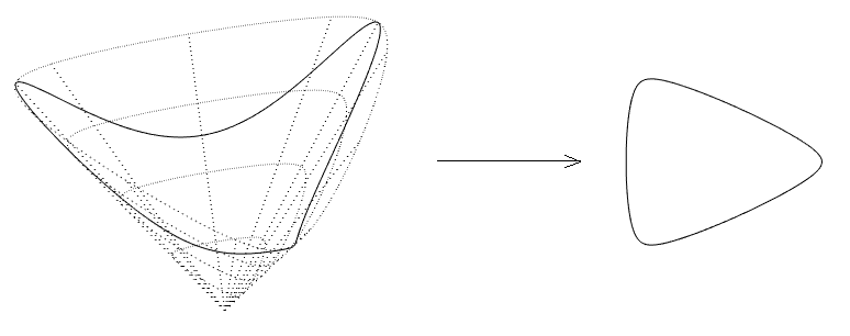
Figure 1: Solution $y(t)$ on the boundary of the cone $K$ and its projection onto the simple closed convex curve $\gamma$ in an affine chart in $\mathbb{R}P^{2}$.

Since the curve $\gamma$ is closed, we may parameterize it $2\pi$-periodically by a variable $t\in\mathbb{R}$. In this case the coefficient functions $\alpha(t),\beta(t)$ are also $2\pi$-periodic. The behaviour of solutions of ODEs with periodic coefficients is the subject of Floquet theory [3]. Namely, a shift of the variable $t$ by $2\pi$ maps the solution space of ODE (3) to itself, and there exists $T\in SL(2,\mathbb{R})$ such that $x(t+2\pi)=Tx(t)$ for all $t\in\mathbb{R}$. The map $T$ is called the monodromy of equation (3). The conjugacy class of the monodromy as well as the winding number of the vector-valued solution $x(t)$ of (3) around the origin over one period are invariant under reparametrizations $t\mapsto s(t)$ of $\gamma$ satisfying $s(t+2\pi)=s(t)+2\pi$, i.e., preserving the periodicity condition [8, pp. 24–25, 34–35].

Equation (3) with periodic coefficient function has been well studied and is known under the name Hill equation. In [6] a complete classification of the coefficient functions under the equivalence relation generated by the group of orientation-preserving diffeomorphisms of $S^{1}$ and a construction of corresponding normal forms has been achieved. The equations can be classified according to several criteria. They may be divided in stable, semi-stable and unstable ones, according to the asymptotic behaviour of the solutions, or into oscillating and non-oscillating ones, according to the behaviour of the argument of the vector-valued solution. Stable solutions are always oscillating. The normal forms of the non-oscillating and the stable equations have constant coefficient functions, while in the remaining cases their coefficient functions are sinusoidal.

In [4] it has been established that the $2\pi$-periodic solutions of equation (4) can be seen as vector fields generating diffeomorphisms of $S^{1}$ which preserve the coefficient function in (3), and at least one non-trivial periodic solution always exists. If such a solution is nowhere zero, then it can be used to construct a diffeomorphism of $S^{1}$ which takes the coefficient function $\alpha$ to a constant. Moreover, this diffeomorphism is unique up to a rotation of $S^{1}$ if and only if $\alpha\not=\frac{n^{2}}{2}$ for all $n\in\mathbb{N}_{+}$. Equations with different values of the constant are non-equivalent.

Our strategy will consist in constructing diffeomorphisms of $S^{1}$ which transform the coefficient function of Hill equation (3) to a constant $\alpha\leq\frac{1}{2}$. In particular, we prove the following result.

Theorem 1.3.

Let $\gamma$ be a simple closed convex projective plane curve of class $C^{k}$, $k\geq 5$, without inflection points. Then there exists a $2\pi$-periodic parametrization of $\gamma$ of class $C^{k-1}$ by a real variable $t$ and a $2\pi$-periodic lift $y:\mathbb{R}\to\mathbb{R}^{3}$ of $\gamma$ of class $C^{k-2}$ such that $y(t)$ is a solution of ODE (2) with $\alpha\equiv const$. Here the value of the constant $\alpha$ is uniquely determined by the curve $\gamma$.

Since the classification results in [6, 4] have been established in the $C^{\infty}$ setting, we shall provide an independent proof.

We shall now briefly summarize the contents of the paper. First we explicitly describe the solution $z(t)$ of the adjoint ODE (5) in terms of $y(t)$ (Lemma 2.1). Next we show that during each period of length $2\pi$ the projective image of the vector-valued solution $w(t)$ of ODE (4) can make at most one turn around the ellipse $\varsigma$ on which it evolves. Equivalently, the solution $x(t)$ of ODE (3) can make at most one half of a turn around the origin (Lemma 2.2). This heavily restricts the behaviour of the solution $x(t)$ (Lemma 2.3) and allows to construct a reparametrization of $\gamma$ which makes the coefficient $\alpha$ constant (Theorem 1.3). The value of the constant $\alpha$ depends on the eigenvalues of the monodromy $T$ of ODE (3) and is hence uniquely determined by the curve $\gamma$. It follows in particular that in general the Forsyth-Laguerre parametrization cannot be extended to the whole closed curve $\gamma$ (Corollary 2.5).

We call a $2\pi$-periodic parametrization of $\gamma$ balanced if the corresponding coefficient function $\alpha$ in (2) is constant.

2 Balanced parametrizations

Let $\gamma$ be a simple closed convex projective plane curve of class $C^{k}$, $k\geq 5$, without inflection points. Let the lift $y(t)$ of $\gamma$ be a $2\pi$-periodic vector-valued solution of ODE (2) such that $\det(y^{\prime\prime},y^{\prime},y)\equiv 1$. The $2\pi$-periodic coefficient functions $\alpha,\beta$ are then of class $C^{k-4},C^{k-5}$, respectively, and $y$ is of class $C^{k-2}$.

Denote $Y=(y^{\prime\prime}+\alpha y,y^{\prime},y)\in SL(3,\mathbb{R})$, then (2) is equivalent to the matrix-valued ODE

$$Y^{\prime}=Y\cdot A_{-},$$ (6)

where for convenience we denoted $A_{\pm}=\begin{pmatrix}0&1&0\\ -\alpha&0&1\\ \pm\beta&-\alpha&0\end{pmatrix}$. We now describe the dual objects in terms of the matrix $Y$.

Lemma 2.1.

Assume above conditions. Let $\gamma^{*}$ the dual projective curve of $\gamma$. There exists a vector-valued solution $z$ of (5) which is a lift of $\gamma^{*}$ and satisfies $\det(z^{\prime\prime},z^{\prime},z)\equiv 1$. The matrix $Z=(z^{\prime\prime}+\alpha z,z^{\prime},z)\in SL(3,\mathbb{R})$ is given by $Z=Y^{-T}Q$ with

$$Q=\begin{pmatrix}0&0&1\\ 0&-1&0\\ 1&0&0\end{pmatrix}.$$

Proof.

Denote the matrix product $Y^{-T}Q$ by $Z$ and let $z$ be its third column. Clearly $Z$ is unimodular and $2\pi$-periodic. In particular, $z$ is non-zero everywhere. Further, by (6) the product $Z$ satisfies the differential equation

$$Z^{\prime}=-Y^{-T}(YA_{-})^{T}Y^{-T}Q=-ZQ^{-1}A_{-}^{T}Q=Z\cdot A_{+}.$$

It follows that $Z=(z^{\prime\prime}+\alpha z,z^{\prime},z)$ and $z$ is a solution of ODE (5). It follows also that $\det(z^{\prime\prime},z^{\prime},z)\equiv 1$. Finally, we have $Y^{T}Z=Q$, which implies $\langle y(t),z(t)\rangle=\langle y^{\prime}(t),z(t)\rangle=0$ for all $t$. Hence the vector $z(t)$ is orthogonal to the plane spanned by $y(t)$ and $y^{\prime}(t)$, and the projective image of $z(t)$ is the corresponding point $\gamma^{*}(t)$ on the dual projective curve. Thus $z$ satisfies all required conditions. ∎

Note that the dual curve $\gamma^{*}$ is also simple closed convex and of class $C^{k}$ without inflection points. Let now $t_{0}\in\mathbb{R}$ and set $y_{0}=y(t_{0})$, $z_{0}=z(t_{0})$. Define the scalar $C^{k-2}$ functions $\mu(t)=\langle y(t),z_{0}\rangle$, $\nu(t)=\langle y_{0},z(t)\rangle$. By convex duality these functions are nonnegative, and $\mu(t)=0$ or $\nu(t)=0$ if and only if $t-t_{0}$ is an integer multiple of the period $2\pi$.

Assume the notations of Lemma 2.1. We have $ZQY^{T}=I$ and hence

$$0 =\langle y_{0},z_{0}\rangle=y_{0}^{T}ZQY^{T}z_{0}=(\nu^{\prime\prime}+\alpha\nu,\nu^{\prime},\nu)Q(\mu^{\prime\prime}+\alpha\mu,\mu^{\prime},\mu)^{T}$$

$$=\nu\mu^{\prime\prime}+2\alpha\nu\mu+\mu\nu^{\prime\prime}-\nu^{\prime}\mu^{\prime}.$$

For $t_{0}<t<t_{0}+2\pi$ define the $C^{k-3}$ functions $\xi=\frac{\mu^{\prime}}{\mu}$, $\theta=\frac{\nu^{\prime}}{\nu}$. Dividing the above relation by $\mu\nu$ and expressing the result in terms of $\xi,\theta$ we obtain

$$\xi^{\prime}+\theta^{\prime}+\xi^{2}-\xi\theta+\theta^{2}+2\alpha=0.$$

Introducing the variable $\psi=\frac{1}{4}(\xi+\theta)$ and taking into account $\xi^{2}-\xi\theta+\theta^{2}=4\psi^{2}+\frac{3}{4}(\xi-\theta)^{2}$ we obtain the differential inequality

$$\psi^{\prime}+\psi^{2}+\frac{\alpha}{2}=-\frac{3}{16}(\xi-\theta)^{2}\leq 0.$$ (7)

Lemma 2.2.

Assume the conditions at the beginning of this section. Let $t_{0}\in\mathbb{R}$ be arbitrary, and let $x(t)$ be a non-trivial scalar solution of ODE (3). Then $x(t)$ cannot have two distinct zeros in the interval $(t_{0},t_{0}+2\pi)$. If $x(t_{0})=x(t_{0}+2\pi)=0$, then $\beta\equiv 0$ and $\gamma$ is an ellipse.

The first assertion follows by virtue of [2, Proposition 9, p. 130] from the existence of a function $\psi(t)$ satisfying (7) on $(t_{0},t_{0}+2\pi)$. We shall, however, give an elementary proof below.

Proof.

Let $t_{m}\in(t_{0},t_{0}+2\pi)$ be arbitrary and define the positive function

$$q(t)=\exp\left(\int_{t_{m}}^{t}\psi(t)\,dt\right)=\left(\frac{\mu(t)\nu(t)}{\mu(t_{m})\nu(t_{m})}\right)^{1/4}$$

on $(t_{0},t_{0}+2\pi)$, where $\psi(t)$ is the function from (7). Then we obtain $q^{\prime\prime}+\frac{\alpha}{2}q=(\psi^{\prime}+\psi^{2}+\frac{\alpha}{2})q\leq 0$.

Let $x(t)$ be an arbitrary non-trivial solution of ODE (3) on $(t_{0},t_{0}+2\pi)$ and consider the function $r(t)=x^{\prime}(t)q(t)-x(t)q^{\prime}(t)$. We have $r^{\prime}=x^{\prime\prime}q-xq^{\prime\prime}=-x(q^{\prime\prime}+\frac{\alpha}{2}q)$.

Suppose for the sake of contradiction that $x(t_{1})=x(t_{2})=0$ for $t_{0}<t_{1}<t_{2}<t_{0}+2\pi$ and $x(t)>0$ for all $t\in(t_{1},t_{2})$. Then $x^{\prime}(t_{1})>0$, $x^{\prime}(t_{2})<0$, and hence $r(t_{1})>0$, $r(t_{2})<0$. But $r^{\prime}(t)\geq 0$ on $(t_{1},t_{2})$, a contradiction. The case when $x(t)$ is negative on $(t_{1},t_{2})$ is treated similarly. This proves the first claim.

Since $t_{0}$ is arbitrary, it follows that no non-trivial solution of ODE (3) can have two consecutive zeros at a distance strictly smaller than $2\pi$.

Let now $x(t)$ be a non-trivial solution of ODE (3) such that $x(t_{0})=x(t_{0}+2\pi)=0$. Then $x(t)$ has constant sign on $(t_{0},t_{0}+2\pi)$, and $r^{\prime}(t)$ is either nonnegative or non-positive, depending on the sign of $x$. In any case the function $r(t)$ is monotonous on $(t_{0},t_{0}+2\pi)$. Note that $q(t)$ and $q^{\prime}(t)$ can be continuously prolonged to $t_{0}$ and $t_{0}+2\pi$ and the limits of $q(t)$ vanish. We hence have $\lim_{t\to t_{0}}r(t)=\lim_{t\to t_{0}+2\pi}r(t)=0$. It follows that $r\equiv 0$, $r^{\prime}\equiv 0$, and therefore $q^{\prime\prime}+\frac{\alpha}{2}q\equiv 0$ on $(t_{0},t_{0}+2\pi)$. But then inequality (7) is actually an equality and $\xi\equiv\theta$. Then there exists a constant $c>0$ such that $\mu\equiv c\nu$. But $\mu(t)$ is a solution of ODE (2), while $\nu(t)$ and hence also $c\nu(t)$ is a solution of (5). Subtracting (5) from (2) with $z,y$ replaced by $\mu$, respectively, we obtain $2\beta(t)\mu(t)=0$ on $(t_{0},t_{0}+2\pi)$. It follows that $\beta\equiv 0$, $y(t)$ is a solution of ODE (4) and hence $\gamma$ is an ellipse. This completes the proof. ∎

Lemma 2.2 allows to restrict the global behaviour of the solutions of ODE (3).

Lemma 2.3.

Assume the conditions at the beginning of this section. Then exactly one of the following cases holds:

• There exists a solution $x(t)$ of ODE (3), normalized such that $\det(x,x^{\prime})\equiv 1$, that is contained in the open positive orthant and crosses each ray of this orthant exactly once, and whose monodromy equals $T=\operatorname{diag}(\lambda^{-1},\lambda)$ for some $\lambda>1$.

• There exists a solution $x(t)$ of ODE (3), normalized such that $\det(x,x^{\prime})\equiv 1$, that is contained in the open right half-plane and crosses each ray of this half-plane exactly once, and whose monodromy equals $T=\begin{pmatrix}1&0\\ 2\pi&1\end{pmatrix}$.

• There exists a solution $x(t)$ of ODE (3), normalized such that $\det(x,x^{\prime})\equiv 1$, that is bounded and turns infinitely many times around the origin, and whose monodromy equals $T=\begin{pmatrix}\cos\varphi&-\sin\varphi\\ \sin\varphi&\cos\varphi\end{pmatrix}$ for some $\varphi\in(0,\pi)$. For every $t_{0}\in\mathbb{R}$ the solution turns by an angle of $\varphi$ around the origin in the interval $[t_{0},t_{0}+2\pi]$.

• There exists a $4\pi$-periodic solution $x(t)$ of ODE (3), normalized such that $\det(x,x^{\prime})\equiv 1$, and whose monodromy equals $T=-I$.

The curve $\gamma$ is an ellipse if and only if case (iv) holds.

Proof.

Let $x(t)$ be an arbitrary solution of ODE (3) with linearly independent components, normalized such that $\det(x,x^{\prime})\equiv 1$. Any other such solution can then be obtained by the action of an element of $SL(2,\mathbb{R})$. The solution $x$ turns counter-clockwise around the origin and intersects every ray transversally.

First we shall treat the case when $\gamma$ is not an ellipse. By Lemma 2.2 every scalar solution of ODE (3) has its consecutive zeros placed at distances strictly larger than $2\pi$. Hence $x$ turns by an angle strictly less than $\pi$ in any time interval of length $2\pi$. In particular, it follows that the solution $x(t)$ cannot cross any 1-dimensional eigenspace of the monodromy $T$. Indeed, suppose that for some $t_{0}\in\mathbb{R}$ the vector $x(t_{0})$ is an eigenvector of $T$. Then $x(t_{0}+2\pi)=Tx(t_{0})$ is a positive or negative multiple of $x(t_{0})$, and $x$ must have made at least half of a turn around the origin in the interval $[t_{0},t_{0}+2\pi]$, a contradiction.

We shall now distinguish several cases according to the spectrum of the monodromy $T$ of ODE (3). Let $T\in SL(2,\mathbb{R})$ be such that $x(t+2\pi)=Tx(t)$ for all $T$. If $\tilde{x}=Ax$ for some $A\in SL(2,\mathbb{R})$, then $\tilde{x}(t+2\pi)=\tilde{T}\tilde{x}(t)$ with $\tilde{T}=ATA^{-1}$. We may hence conjugate $T$ with an arbitrary unimodular matrix by switching to another solution $x$.

Case 1: The eigenvalues of $T$ are given by $\lambda,\lambda^{-1}$ for some $\lambda>1$. By conjugation with a unimodular matrix we may achieve $T=\operatorname{diag}(\lambda^{-1},\lambda)$. Since $x(t)$ cannot cross the axes, it must be confined to an open quadrant. For every point $q$ in the second or fourth open quadrant the vector $Tq$ has a polar angle strictly less than that of $q$. But $x(t)$ turns in the counter-clockwise direction, and hence cannot be contained in these quadrants. By possibly multiplying $x$ by $-1$ we may hence achieve that $x$ is contained in the open positive orthant. Now for any $t_{0}\in\mathbb{R}$ the angles of the vectors $T^{k}x(t_{0})$ tend to $\frac{\pi}{2}$ and those of $T^{-k}x(t_{0})$ to 0 as $k\to+\infty$. Therefore the angles of $x(t)$ sweep the interval $(0,\frac{\pi}{2})$ as $t$ sweeps the real line. This is the situation described in case (i) of the lemma.

Case 2: The eigenvalues of $T$ equal 1. Since $x(t)$ cannot be an eigenvector of $T$ for any $t$, we must have $T\not=I$ and the Jordan normal form of $T$ contains a single Jordan cell. By conjugation with a unimodular matrix we may then achieve that $T=\begin{pmatrix}1&0\\ \pm 2\pi&1\end{pmatrix}$. Since $x(t)$ cannot cross the vertical axis, it must be contained in the left or right open half-plane. By multiplying by $-1$ we may assume the solution is contained in the right half-plane. Now if the $(2,1)$ element in $T$ equals $-2\pi$, then for every point $q$ in the open right half-plane the vector $Tq$ has a polar angle strictly less than that of $q$. This is in contradiction with the counter-clockwise movement of $x$, and this case cannot appear. Hence the $(2,1)$ element in $T$ equals $2\pi$. Then for any $t_{0}\in\mathbb{R}$ the angles of the vectors $T^{k}x(t_{0})$ tend to $\frac{\pi}{2}$ and those of $T^{-k}x(t_{0})$ to $-\frac{\pi}{2}$ as $k\to+\infty$. Therefore the angles of $x(t)$ sweep the interval $(-\frac{\pi}{2},\frac{\pi}{2})$ as $t$ sweeps the real line. This is the situation described in case (ii) of the lemma.

Case 3: The eigenvalues of $T$ equal $e^{\pm i\varphi}$ for $\varphi\in(0,\pi)$. By conjugation with an element in $SL(2,\mathbb{R})$ we may achieve that $T=\begin{pmatrix}\cos\varphi&\mp\sin\varphi\\ \pm\sin\varphi&\cos\varphi\end{pmatrix}$. If the $(2,1)$ element of $T$ has negative sign, then for every $q\not=0$ the angle of $Tq$ equals $2\pi-\varphi$ plus the angle of $q$. Since $x$ moves counter-clockwise, it must hence sweep an angle of at least $2\pi-\varphi>\pi$ on any interval of length $2\pi$, which is not possible. Hence the $(2,1)$ element of $T$ has positive sign, and for every $q\not=0$ the angle of $Tq$ equals $\varphi$ plus the angle of $q$. Since $x$ cannot make a complete turn around the origin in an interval of length $2\pi$, the angle swept by the solution on any such interval equals $\varphi$. Finally note that since $T$ acts by a rotation, the norm of the solution $x$ is $2\pi$-periodic and hence uniformly bounded. This is the situation described in case (iii) of the lemma.

Case 4: The eigenvalues of $T$ equal $-1$. Similarly to Case 2 we have $T\not=-I$, and the Jordan normal form of $T$ consists of a single Jordan cell. The eigenspace to the eigenvalue $-1$ then divides $\mathbb{R}^{2}$ in two half-planes. For every $q$ in one of the open half-planes, the point $Tq$ lies in the other open half-plane. Hence the solution $x(t)$ must cross the eigenspace, leading to a contradiction. Hence this case does not occur.

Case 5: The eigenvalues of $T$ equal $-\lambda,-\lambda^{-1}$ for some $\lambda>1$. By conjugation with a unimodular matrix we may achieve $T=\operatorname{diag}(-\lambda^{-1},-\lambda)$. Similarly to Case 1 the solution $x(t)$ must then be contained in some open quadrant. But the map $T$ maps every quadrant to the opposite quadrant. Hence $x$ must cross the axes, which leads to a contradiction. Thus this case does not occur either.

We now consider the case when $\gamma$ is an ellipse. By Lemma 2.2 we have $\beta\equiv 0$ and (2), (4) represent the same ODE. Since all solutions $y$ of ODE (2) are $2\pi$-periodic, the solutions $w$ of (4) are also $2\pi$-periodic. But the solutions $w$ are homogeneous quadratic functions of the solutions $x$ of ODE (3). Hence the latter are $4\pi$-periodic, and $T^{2}=I$. If $T=I$, then every two consecutive zeros of every non-trivial scalar solution of ODE (3) have a distance strictly smaller than $2\pi$, leading to a contradiction with Lemma 2.2. Hence $T=-I$, and we are in the situation described in case (iv) of the lemma.

This completes the proof. ∎

Remark 2.4.

The cases i) — iv) in the formulation of the lemma correspond to the unstable non-oscillating, semi-stable non-oscillating, stable with $\Theta<1$, and stable with $\Theta=1$ cases, correspondingly, in the classification in [6]. The cases 4 and 5 in the proof correspond to the semi-stable and unstable oscillating cases in [6].

Corollary 2.5.

Assume the conditions at the beginning of this section. If the eigenvalues of the monodromy of ODE (3) differ from 1, then the curve $\gamma$ does not possess a global periodic Forsyth-Laguerre parametrization.

Proof.

Suppose $\gamma$ possesses a periodic Forsyth-Laguerre parametrization by a variable $s$. In this parametrization any non-zero vector-valued solution $\tilde{x}(s)$ of ODE (3) with independent components is a straight affine line, and hence sweeps a total angle of $\pi$ in the plane.

Let now $\gamma$ be parameterized $2\pi$-periodically by a variable $t$. Every non-zero vector-valued solution $x(t)$ of ODE (3) with independent components must also sweep a total angle of $\pi$. From Lemma 2.3 it follows that the monodromy of ODE (3) has eigenvalues equal to 1. ∎

We are now in a position to construct the reparametrization $t\mapsto s(t)$ which makes the coefficient $\alpha$ in ODE (2) constant.

of Theorem 1.3.

We shall begin with an arbitrary regular $2\pi$-periodic parametrization of $\gamma$ of class $C^{k}$. As laid out in Section 1, there exists a $2\pi$-periodic lift $y(t)$ of $\gamma$ which solves ODE (2) with some $2\pi$-periodic functions $\alpha(t)$, $\beta(t)$ of class $C^{k-4},C^{k-5}$, respectively. The coefficient function $\alpha$ gives rise to ODE (3). We shall construct a $2\pi$-periodic parametrization of $\gamma$ by a new variable $s$ from the vector-valued $C^{k-2}$ solutions $x(t)=(x_{1}(t),x_{2}(t))$ of ODE (3) described in Lemma 2.3. Note that if we write $x_{1}=r\cos\phi$, $x_{2}=r\sin\phi$, then the condition $\det(x,x^{\prime})\equiv 1$ implies $r^{2}\phi^{\prime}\equiv 1$ and $\phi^{\prime}=r^{-1/2}$. Since $r(t)$ is of class $C^{k-2}$, the angle $\phi$ is of class $C^{k-1}$. We consider the four cases (i) — (iv) in Lemma 2.3 separately.

Case (i): Set $s(t)=\frac{\pi}{\log\lambda}\log\frac{x_{2}(t)}{x_{1}(t)}$. Note that $s$ is an analytic function of the angle $\phi$ and hence $s(t)$ is a $C^{k-1}$ function. We have $s(t+2\pi)=\frac{\pi}{\log\lambda}\log\frac{\lambda x_{2}(t)}{\lambda^{-1}x_{1}(t)}=s(t)+2\pi$, and the new parameter $s$ parameterizes $\gamma$ $2\pi$-periodically. Set further $c=\frac{\pi}{\log\lambda}>0$ and $\tilde{\alpha}=-\frac{1}{2c^{2}}<0$. Then the vector-valued function $\tilde{x}(s)=(\sqrt{c}\lambda^{-s/2\pi},\sqrt{c}\lambda^{s/2\pi})$ obeys the differential equation $\frac{d^{2}\tilde{x}}{ds^{2}}+\frac{\tilde{\alpha}}{2}\tilde{x}=0$ and we have $\frac{\tilde{x}_{2}(s(t))}{\tilde{x}_{1}(s(t))}=\lambda^{s(t)/\pi}=\frac{x_{2}(t)}{x_{1}(t)}$ for all $t$. Moreover, $\det(\tilde{x},\frac{d\tilde{x}}{ds})\equiv 1$. By Corollary 1.2 the coefficient $\alpha$ in ODE (2) in the new coordinate $s$ identically equals the constant $\tilde{\alpha}$. The coefficient $\beta$ in the new variable is given by $\tilde{\beta}(s)=\beta(t)(\frac{ds}{dt})^{-3}$, because $\beta$ transforms as the coefficient of a cubic differential. Hence $\tilde{\beta}(s)$ is as $\beta(t)$ a $C^{k-5}$ function. Therefore the solution $\tilde{y}(s)$ of ODE (2) in the variable $s$ is of class $C^{k-2}$.

Case (ii): Set $s(t)=\frac{x(t_{2})}{x(t_{1})}$. Again $s$ is an analytic function of the angle $\phi$ and $s(t)$ is a $C^{k-1}$ function. We have $s(t+2\pi)=\frac{2\pi x(t_{1})+x(t_{2})}{x(t_{1})}=s(t)+2\pi$, and $s$ parameterizes $\gamma$ $2\pi$-periodically. Define $\tilde{x}(s)=(1,s)$, then $\det(\tilde{x},\frac{d\tilde{x}}{ds})\equiv 1$, $\frac{d^{2}\tilde{x}}{ds^{2}}=0$, and $\frac{\tilde{x}_{2}(s)}{\tilde{x}_{1}(s)}=\frac{x(t_{2})}{x(t_{1})}$. By Corollary 1.2 the coefficient $\alpha$ in ODE (2) in the new coordinate $s$ identically equals zero. As in the previous case the coefficient $\tilde{\beta}(s)$ is a $C^{k-5}$ function and the solution $\tilde{y}(s)$ of ODE (2) in the variable $s$ is of class $C^{k-2}$.

Case (iii): Set $s(t)=\frac{2\pi}{\varphi}\phi(t)$. Again $s$ is a $C^{k-1}$ function and $s(t+2\pi)=\frac{2\pi}{\varphi}(\phi(t)+\varphi)=s(t)+2\pi$, and $s$ parameterizes $\gamma$ $2\pi$-periodically. Define $c=\frac{2\pi}{\varphi}$, $\tilde{\alpha}=\frac{2}{c^{2}}$, and $\tilde{x}(s)=(\sqrt{c}\cos\frac{s}{c},\sqrt{c}\sin\frac{s}{c})$. Then $\det(\tilde{x},\frac{d\tilde{x}}{ds})\equiv 1$, $\frac{d^{2}\tilde{x}}{ds^{2}}+\frac{\tilde{\alpha}}{2}\tilde{x}=0$, and the angles of $x(t)$ and $\tilde{x}(s)$ both equal $\phi$. By Corollary 1.2 the coefficient $\alpha$ in ODE (2) in the new coordinate $s$ identically equals the constant $\tilde{\alpha}$. As in the previous case the coefficient $\tilde{\beta}(s)$ is a $C^{k-5}$ function and the solution $\tilde{y}(s)$ of ODE (2) in the variable $s$ is of class $C^{k-2}$.

Case (iv): The curve $\gamma$ is an ellipse, and by an appropriate choice of the coordinate basis in $\mathbb{R}^{3}$ we may achieve that $\gamma$ is the projective image of the vector-valued function $y(t)=(1,\cos t,\sin t)$. This function is a solution of ODE (2) with $\alpha\equiv\frac{1}{2}$, $\beta\equiv 0$, and the variable $t$ parameterizes $\gamma$ analytically and $2\pi$-periodically.

Finally we show that the value of the constant $\alpha$ is uniquely determined by $\gamma$. Let the lift $y(t)$ of $\gamma$ be a $2\pi$-periodic solution of ODE (2) with constant coefficient $\alpha$. Let $x(t)$ be the solution from Lemma 2.3.

If $\alpha<0$, then $x(t)$ must be a hyperbola, hence case (i) is realized, and $\alpha$ relates to the spectrum of the monodromy $T$ of ODE (3) by $\alpha=-\frac{\log^{2}\lambda}{2\pi^{2}}$.

If $\alpha=0$, then by Corollary 2.5 the eigenvalues of $T$ equal 1.

If $\alpha\in(0,\frac{1}{2})$, then $x(t)$ must be an ellipse and sweeps an angle strictly less than $\pi$ in any interval of length $2\pi$. Hence case (iii) is realized, and $\alpha$ is related to the spectrum of $T$ by $\alpha=\frac{\varphi^{2}}{2\pi^{2}}$.

If $\alpha\geq\frac{1}{2}$, then $x(t)$ must also be an ellipse and sweeps an angle of at least $\pi$ in any interval of length $2\pi$. Hence case (iv) is realized, $x(t)$ sweeps an angle of exactly $\pi$, and $\alpha=\frac{1}{2}$.

In any case $\alpha$ is uniquely determined by the spectrum of $T$. However, the spectrum of $T$ depends only on $\gamma$. Hence $\alpha$ is also uniquely determined by $\gamma$. ∎

Definition 2.6.

Let $\gamma$ be a simple closed convex projective plane curve of class $C^{k}$, $k\geq 5$, without inflection points. We call a $2\pi$-periodic parametrization of $\gamma$ by a real variable $t$ balanced if there exists a $2\pi$-periodic lift $y(t)$ of $\gamma$ to $\mathbb{R}^{3}$ which is a vector-valued solution of ODE (2) with $\alpha\equiv const$.

By Theorem 1.3 a balanced parametrization always exists. In the case of non-quadratic curves the balanced parametrization is unique up to a shift of the variable $t$ by [4, Lemma 2], and hence defines an invariant metric on the curve. For an ellipse every two balanced parametrizations are related by a projective transformation.

References

- [1] Elie Cartan. Leçons sur la théorie des espaces à connexion projective. Gauthiers-Villars, Paris, 1937.
- [2] C. de la Vallée Poussin. Sur l’équation différentielle linéaire du second ordre. J. Math. Pure Appl., 8:125–144, 1929.
- [3] Gaston Floquet. Sur les équations différentielles linéaires à coefficients périodiques. Annales de l’Ecole Normale Supérieure, 12:47–88, 1883.
- [4] Alexandre A. Kirillov. Infinite dimensional Lie groups; their orbits. Invariants and representations. The geometry of moments, pages 101–123. Number 970 in Lect. Notes Math. Springer, 1982.
- [5] Nicholaas H. Kuiper. Locally projective spaces of dimension 1. Michigan Math. J., 2:95–97, 1953.
- [6] V.F. Lazutkin and T.F. Pankratova. Normal forms and versal deformations for Hill’s equation. Funct. Anal. Appl., 9:306–311, 1975.
- [7] S. Mukhopadhyaya. New methods in the geometry of a plane arc I. Bull. Calcutta Math. Soc., 1:31–37, 1909.
- [8] V. Ovsienko and S. Tabachnikov. Projective geometry old and new, volume 165 of Cambridge Tracts in Mathematics. Cambridge University Press, Cambridge, 2005.
- [9] Gudlaugur Thorbergsson and Masaaki Umehara. Sextactic points on a simple closed curve. Nagoya Math. J., 167:55–94, 2002.
- [10] E.J. Wilczynski. Projective differential geometry of curves and ruled surfaces. Teubner, Leipzig, 1906.