UV background fluctuations traced by metal ions at $z\approx 3$

Abstract

Here we investigate how LyC-opaque systems present in the intergalactic medium at $z\approx 3$ can distort the spectral shape of a uniform UV background (UVB) through radiative transfer (RT) effects. With this aim in mind, we perform a multi-frequency RT simulation through a cosmic volume of $10h^{-1}$ cMpc scale polluted by metals, and self-consistently derive the ions of all the species. The UVB spatial fluctuations are traced by the ratio of He$\,\rm\scriptstyle II\$ and H$\,\rm\scriptstyle I\$ column density, $\eta$, and the ratio of C$\,{\rm{\scriptstyle IV\ }}$ and Si$\,{\rm{\scriptstyle IV\ }}$ optical depths, $\zeta$. We find that: (i) $\eta$ spatially fluctuates through over-dense systems ($\Delta$) with statistically significant deviations $\delta\eta>25$% in 18% of the volume ; (ii) same fluctuations in $\zeta$ are also present in $34$% of the enriched domain (only 8% of the total volume) and derive from a combination of RT induced effects and in-homogeneous metal enrichment, both effective in systems with $\Delta>1.5$.

1 INTRODUCTION

Since the first observations, the He$\,{\rm{\scriptstyle II\ }}$ opacity of the intergalactic medium (IGM) at $z\approx 3$ has been interpreted as “patchy” and highly in-homogeneous (Reimers et al., 1997; Hogan et al., 1997; Heap et al., 2000; Smette et al., 2002; Syphers et al., 2011; Syphers & Shull, 2014), as highlighted by the Ly-$\alpha$ forest parameter $\eta$. In a photo-ionised IGM, $\eta$ is proportional to the UV background spectral shape (UVBSS) and its scatter in space could reflect spatial fluctuations of the UVB at the ionisation edges of H$\,{\rm{\scriptstyle I\ }}$ and He$\,{\rm{\scriptstyle II\ }}$ (Miralda-Escude, 1993). In the last twenty years different interpretations were provided on the origin of these fluctuations. Spectroscopic observations reported variations of $\eta\in[20-200]$ over scales of $\left[2\text{\textendash}10\right]$ Mpc (Shull et al., 1999; Fardal et al., 1998; Fechner & Reimers, 2007), which could be interpreted as a local ionisation effect in the proximity of quasars (Shull et al., 2004, 2010; Worseck et al., 2007). A decrease of $\eta$ in redshift, on the other hand, could indicate an evolution in the UVBSS (Zheng et al., 2004). Optical depth ratios from metal lines have been often suggested as additional/independent probes of UVBSS spatial variations: $\zeta\equiv\tau_{\textrm{SiIV}}/\tau_{\textrm{CIV}}$ for example, is sensitive to the UVBSS on either side of the He$\,{\rm{\scriptstyle II\ }}$ ionisation edge (Songaila et al., 1995; Songaila & Cowie, 1996; Giroux & Shull, 1997; Savaglio et al., 1997; Songaila, 1998) and to $[\texttt{Si}/\texttt{C}]$. This optical depth ratio was observed to abruptly change around $z=3$ by Songaila (1998) and interpreted as a sudden hardening of the UVB; a redshift evolution of $\zeta$ was also found by Agafonova et al. (2005); Agafonova et al. (2007) and Levshakov et al. (2008). Independent measurements, on the other hand, did not confirm the previous findings (Kim et al., 2002; Aguirre et al., 2004). Thus far observations are too scarce to draw a definitive conclusion on the amplitude of the UVBSS fluctuations and on their significance level (e.g. see McQuinn & Worseck 2014 for a case against fluctuations).

Most models of the UVB are not suitable to address this problem because they are generally limited by the assumption of spatial homogeneity and do not account for RT effects, important when density contrasts are present (Maselli & Ferrara 2005, hereafter MF05; Bolton et al. 2006; McQuinn 2009; Ciardi et al. 2012; Meiksin & Tittley 2012; Davies & Furlanetto 2014; Davies et al. 2017). Bolton and Viel (2011, hereafter BV11) adopted a set of spatially in-homogeneous UVB models confirming fluctuations in $\eta$ but they did not find any significant difference in the values of $\zeta$ across models.

By performing a RT simulation of a spatially uniform UVB through a realistic cosmic web polluted by metals, here we show that both random gas clumps of the IGM and RT effects can induce spatial fluctuations in the UVBSS. These distortions are traced as scatter in space of $\eta$ and $\zeta$ and computed by the new features of the cosmological RT code CRASH3 (Graziani et al. 2013, hereafter GR13). We find that: (i) non negligible spatial oscillations of $\eta$ and $\zeta$ come naturally from both RT effects and in-homogeneous distribution in space of gas over-densities $\Delta$; (ii) $\zeta$ can be used as tracer of UVBSS in the metal enriched sub-domain but one has to be aware of the fact that it suffers the complex interplay between radiative and chemical feedback.

This paper is structured as follows. In Section 2 we introduce the numerical simulations, while Section 3 discusses the fluctuations in $\eta$ and $\zeta$. Section 4 finally summarizes the conclusions.

2 Numerical simulations

The galaxy formation simulation adopted in this work was performed on a box of $10h^{-1}$ Mpc comoving by using a modified version of the GADGET-2 code (Springel, 2005), as described in Maio et al. (2010). The code includes the whole set of chemistry reactions leading to molecule creation and destruction, as well as metal production and spreading. Metals are released by AGB stellar winds and supernovae (SNII, SNIa) explosions following star formation and according to the stellar lifetimes and production yields. They are successively spread over the neighbours of stellar particles according to the SPH kernel (Tornatore et al., 2007) within a kinetic feedback scheme accounting for winds with velocity of 500 km s^-1. A cosmic UVB (Haardt & Madau 1996, hereafter HM96) is also included as photo-ionisation radiation field.

One density snapshot at redshift $z\approx 3$ was ionized after mapping gas and metals on a Cartesian grid of resolution $N_{c}^{3}=128^{3}$ cells. Its cosmic web is enriched in $\approx 23$% of the total domain: $\approx 17$% has metallicity $Z<0.1Z_{\odot}$, while only $\approx 1$% has $Z>1Z_{\odot}$. The contribution of metals to the gas cooling function adopted in the RT simulation is also accounted for, as described in GR13.

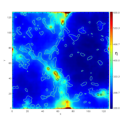
Figure 1: Slice cut through the simulation box showing the spatial distribution of $\eta$ at the equilibrium time $t_{eq}$. The distance in the x- and y-axis is shown in cell units (1 cell $\approx 78$ h^-1 ckpc), the depth of the slice is 1 cell. Iso-contour lines refer to $\Delta\approx 1$ (white solid), $\Delta\approx 5$ (black dashed), $\Delta\approx 10$ (black solid).

For consistency with the hydrodynamic simulation, CRASH3 adopts a HM96 UVB sampled by emitting $10^{4}$ photon packets from $32^{3}$ grid nodes uniformly covering the cosmic volume. The HM96 spectral shape, defined as $J(\nu)/J_{912}$ , is sampled by $101$ bins, more concentrated around the ionisation frequencies of H and He and extends up to $\nu_{\texttt{max}}\approx 124$ Å($E_{\nu,\texttt{max}}\approx 100$ eV) to allow a direct comparison with the MF05 results. During the run it is tracked in regions with $Z>0$ to derive metal ions with the CLOUDY (v.10, Ferland et al. 1998) module embedded in CRASH3. Periodic boundary conditions are set up by reusing the escaping packets 10 times to approximately cover the mean free path of ionising photons at $z=3$ ($\approx 100h^{-1}$ cMpc, Fan et al. 2002). The simulation starts from a neutral gas at $T_{0}=100$ K and proceeds until an ionisation equilibrium is reached ($t_{eq}=5.5\cdot 10^{6}$ yr). The resulting volume averaged ionisation fractions are $\overline{x}_{\texttt{HII}}\approx 0.999997$, $\overline{x}_{\textrm{HeII}}\approx 0.036899$ and $\overline{x}_{\textrm{HeIII}}\approx 0.963097$

3 Results

Here we show the spatial fluctuations of $\eta$ and $\zeta$ at $t_{eq}$ and we study them as function of $\Delta$. The relative fluctuation of $\eta$ (or $\zeta$) around the highest probability value ($\eta_{p}$) of its distribution is defined as $\delta\eta\equiv\left|\dfrac{\eta-\eta_{p}}{\eta_{p}}\right|$, while $\overline{\eta}$ indicates the volume averaged value. The statistical distributions of both quantities are computed in all the cells in which they are investigated, i.e. the cosmic volume for $\eta$ and the over-dense, metal polluted domain for $\zeta$.

3.1 Fluctuations of $\eta$

To compute $\eta$ at simulation run-time we adopt the notation of Fardal et al. (1998):

$$\eta=\frac{\alpha_{\textrm{HeII}}(T)}{\alpha_{\textrm{HI}}(T)}\frac{n_{\textrm{HeIII}}}{n_{\textrm{HII}}}\frac{\Gamma_{\textrm{HI}}}{\Gamma_{\textrm{HeII}}},$$ (1)

where $\alpha_{\textrm{HeII}}$ and $\alpha_{\textrm{HI}}$ are the Case A He$\,{\rm{\scriptstyle II\ }}$ and H$\,{\rm{\scriptstyle I\ }}$ recombination coefficients, while $\Gamma_{\textrm{HeII}}$ and $\Gamma_{\textrm{HI}}$ are their photo-ionisation rates computed in each cell of the domain.

In Figure 1 we show $\eta$ in a slice with a central over-dense filament enriched by metals. The under-dense regions ($\approx 33$% of the plane, dark-blue areas) are characterized by $\eta\approx 260$, while the central filament shows values in the range $350<\eta<450$. Higher values, up to $\eta=600$, are found instead in the densest clumps visible at the borders of the figure. To highlight the tight correlation between $\eta$ and $\Delta$, we over-plot $\Delta$ iso-contour lines. As argued in MF05, at photo-ionisation equilibrium $\eta$ increases with $\Delta$ for a combination of reasons: (i) the recombination rates show a weak dependence on $T$ and then the ratio is expected to weakly reflect the increase of $T$ in $\Delta>1$ (Theuns et al., 1998); (ii) helium recombines $5.5$ times faster than hydrogen and in over-dense regions the ratio $\frac{n_{\textrm{HeII}}}{n_{\textrm{HI}}}$ drives the increase of $\eta$ with $\Delta$ as the Universe is more opaque in He$\,{\rm{\scriptstyle II\ }}$; (iii) $\Gamma_{\textrm{HI}}$ is always one order magnitude larger than $\Gamma_{\textrm{HeII}}$. Note that spatial fluctuations in $T$ are also present and will be investigated in a companion paper.

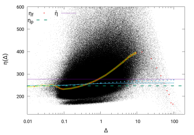
Figure 2: Scatter plot of $\eta$ (black points) as function of $\Delta$ at the equilibrium time $t_{eq}$. The average value at fixed $\Delta$, $\eta_{f}$, is shown as red crosses, while the highest probability value $\eta_{p}$ in the volume as dashed green line and the volume average value $\overline{\eta}$ as violet solid line. The yellow shadow area indicates the average noise in $\eta_{f}$ intrinsic in our RT algorithm. Finally, dotted (solid) light-blue lines show the values of $\eta_{\texttt{eq}}(\Delta,Z)$ assuming a uniform HM96 UVB and gas metallicity $Z=0.01$ Z_⊙ ($Z=3$ Z_⊙).

Figure 2 shows, as scatter plot, the values of $\eta$ found in each cell of the cosmic volume as function of their over-density $\Delta$. The average of $\eta$ at fixed over-density (${\eta_{f}}$) is also shown as reference with red crosses. The yellow transparent area indicates the effects of the CRASH3 numerical noise on $\eta$, evaluated by propagating a spatially homogeneous UVB through a medium with constant number density ; the fluctuations induced on $\eta$ by that noise are always lower than 1.5% in all tests. A significant scatter is found around each ${\eta_{f}}$ (red crosses) and around both $\eta_{p}$ (violet solid line) and $\overline{\eta}$ (dashed green line), computed from the global statistic. Note that regions with $\Delta<0.1$ exhibit a low scatter at fixed number density: 5-8% around ${\eta_{f}}\approx 252$, with only few cells reaching 15%. In $0.1<\Delta\leq 10$, $\eta_{f}$ increases with $\Delta$ and the scatter shows typical statistically significant variations of 20-30%, with values as high as 60% in the range $7\leq\Delta\leq 10$. As discussed in MF05, in very dense regions with $\Delta>10$ recombination dominates over ionisation, inducing an inversion of the trend, with $\eta_{f}$ decreasing with increasing $\Delta$. Finally note that the small cloud of points in which $\eta<200$ ($0.1<\Delta<10$) is created by cells hosting photon emission nodes. In these cells in fact our ionization algorithm tends to fully ionize the gas and to lower the value of $\eta$; their total number is, on the other hand, lower than 1% with a negligible impact on the global statistic. As a comparison, we computed $\eta_{\texttt{eq}}(\Delta,Z)$, i.e. the value of $\eta$ determined by Cloudy photo-ionisation equilibrium models assuming a spatially homogeneous HM96 UVB, as described in Section 2. All $\eta_{\texttt{eq}}(\Delta,Z)$ lie between the values corresponding to the min/max of the gas metallicity ($0.01$ Z_⊙, dotted; $3$ Z_⊙, solid light-blue lines). In under-dense regions $\eta_{\texttt{eq}}\approx\eta_{f}$ because the RT effects are minimized and $Z$ is usually low. $\eta_{\texttt{eq}}$ slightly increases with $\Delta$ at all $Z$ remaining confined in $\eta_{p}<\eta_{\texttt{eq}}(\Delta)<\overline{\eta}$; the divergence between dotted and solid light-blue lines is caused by the decrease of $T$ at increasing $Z$ but with modest effects because $\alpha_{\textrm{HeII}}/\alpha_{\textrm{HI}}\propto(T/10^{4.3})^{0.06}$. Finally note that at $\Delta>1$ the RT effects become important and then $\eta_{\texttt{eq}}$ rapidly separate from $\eta_{f}$.

The statistical distribution of $\eta$ shows $\eta_{p}\approx 247$ and $\overline{\eta}\approx 277$. In $\approx 82$% of the domain $\delta\eta\leq 25$%, while a fluctuation within $25$%$<\delta\eta\leq 50$% is found in 11% of the cells. Finally, values in $50$%$<\delta\eta\leq 75$% are found in 4% of the domain and a remaining 3% shows $\delta\eta>75$%.

The above results are in global agreement with MF05, but it should be noted that our statistic shows higher fluctuations when $\Delta>1$ due to the improved feedback model of the hydrodynamical simulation, which creates sharper density gradients and enhances the RT effects. As a result, the spatial UVB fluctuations increase. Finally, we point out that while our analysis is not meant to quantitatively reproduce observations (this will be addressed in a companion project with an updated UVB model, i.e. Haardt & Madau 2012), the predicted value of $\overline{\eta}\approx 277$ is consistent with the one observed in Heap et al. (2000) and Syphers & Shull (2014) at $z\approx 3$. Our fluctuation range is reasonable as well, as it is consistent with the estimates in Shull et al. (2004) inferred at a similar scale (i.e $10h^{-1}$ Mpc comoving), although it is in tension with values found in McQuinn & Worseck (2014). Note, though, that the latter results refer to lower redshift data ($z<2.7$), where the progress of reionization could have significantly reduced the fluctuations of $\eta$.

3.2 Fluctuations of $\zeta$

Here we discuss the scatter in $\zeta$, which provides an additional evidence of the UVBSS spatial fluctuations using metal ions. Since CRASH3 does not include the metal contribution to the gas optical depth (see GR13 for more details), $\zeta$ computed in this paper fluctuates as a result of absorption by H and He only, and of in-homogeneous chemical enrichment. Spectral distortions around the ionisation energy of H$\,{\rm{\scriptstyle I\ }}$ and He$\,{\rm{\scriptstyle II\ }}$ impact in fact the ionization of both Si$\,{\rm{\scriptstyle IV\ }}$ and C$\,{\rm{\scriptstyle IV\ }}$ and alter the ratio of their ionization fractions. In addition, fluctuations of $[\texttt{Si}/\texttt{C}]$ are expected in different density environments because metals are followed individually during their spreading outside the formation sites. For an easier comparison with BV11, we compute $\zeta$ in each cell of the over-dense, polluted volume as:

$$\zeta=1.7\frac{x_{\texttt{SiIV}}}{x_{\texttt{CIV}}}10^{[\texttt{Si}/\texttt{C}]-0.77},$$ (2)

where $x_{\texttt{SiIV}}$ and $x_{\texttt{CIV}}$ are the ionization fractions of Si$\,{\rm{\scriptstyle IV\ }}$ and C$\,{\rm{\scriptstyle IV\ }}$, respectively. $\zeta$ can then be studied as a combination of two terms: $x\equiv x_{\texttt{SiIV}}/x_{\texttt{CIV}}$ (mainly affected by RT) and $y\equiv 10^{[\texttt{Si}/\texttt{C}]-0.77}$, reflecting the in-balance of atom abundances created by mechanical and chemical feedback. Hereafter we focus on the sub-domain $\Delta>1.5$ because it is significantly metal polluted and simultaneously shows large fluctuations in the UVB spectral shape through $\eta$.

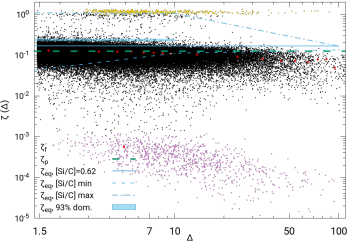
Figure 3: Scatter plot of $\zeta$ (black points) as function of $\Delta$ at $t_{eq}$. The average value at fixed $\Delta$, $\zeta_{f}$, is shown as red crosses, while the highest probability value $\zeta_{p}$ as dashed green line. Violet points indicate cells in which $x\equiv x_{\texttt{SiIV}}/x_{\texttt{CIV}}<10^{-3}$, while gold points mark cells in which $x=1$. Dashed/dashed-dotted light-blue lines show $\zeta_{\texttt{eq}}(\Delta,[\texttt{Si}/\texttt{C}])$ computed at the minimum/maximum values of $[\texttt{Si}/\texttt{C}](\Delta)$, while a case at the highest probability value of $[\texttt{Si}/\texttt{C}](1.5)\approx 0.62$ is shown as a solid line. Finally note that in about 93% of the domain $1.5\leq\Delta<10$, $\zeta_{\texttt{eq}}$ has values in the cyan shadow area.

Figure 3 shows the scatter plot of $\zeta(\Delta)$. Deviations of $\zeta$ from $\zeta_{f}$ are present everywhere, but contrary to $\eta$ there is no tight dependence on $\Delta$ and $\zeta_{f}$ decreases of about 25% from $\Delta<7$ ($\zeta_{f}\approx 0.125$) to higher over-densities where $\zeta_{f}\approx 0.1$. Large fluctuations (up to several orders of magnitude) are clearly visible around any $\zeta_{f}$, but when a statistically significant number of cells is considered their amplitude reduces to $\approx$60%. In specific cases (see the cloud of violet points) $\zeta$ scatters in $10^{-5}<\zeta<10^{-3}$ because of the extremely low values of $x$ ($x<10^{-3}$), i.e. either the spectral shape created in these cells is highly altered by absorption at the ionization potential of Si$\,{\rm{\scriptstyle IV\ }}$ ($\approx 45$ eV) or a hard spectrum generates higher ionization states (see for example the model UVB3 studied in BV11). Another limited set of points (gold cloud) is determined by the conditions: $x=1$, and $y$ almost constant. In these cells either Si$\,{\rm{\scriptstyle IV\ }}$ and C$\,{\rm{\scriptstyle IV\ }}$ are fully ionized or in ionization states higher than IV. As in Figure 2, the light-blue lines refer to $\zeta_{\texttt{eq}}(\Delta,[\texttt{Si}/\texttt{C}])$ computed by assuming a uniform UVB. At constant $[\texttt{Si}/\texttt{C}](1.5)\approx 0.62$ (i.e. $y(\Delta)\approx 0.7$, solid line), $\zeta_{\texttt{eq}}(\Delta)$ shows a global decrease of only 4%, driven by a decrease of $x$ with increasing $\Delta$. When the UVB is assumed homogeneous in space, the only term inducing significant spatial fluctuations is then $y$. By adopting the min/max values of $y(\Delta)$ we can trace the dashed/dashed-dotted lines, also showing that the maximum variation of $[\texttt{Si}/\texttt{C}]$ is found in $1.5<\Delta<10$, while it significantly reduces at higher over-density. These extreme cases, on the other hand, must be taken with a grain of salt as they are found in less than 7% of the cells; the scatter of $[\texttt{Si}/\texttt{C}]$ from the average value is $\leq 4$% in the remaining 93%, i.e. $\zeta_{\texttt{eq}}$ is confined in the cyan shadow area..

In Figure 4 we show the statistic of $\zeta$ computed over $N_{c}^{3}$ cells (total domain, solid blue lines) and over the total number of cells polluted by metals (polluted domain, dashed blue lines); in this way the reader can have a feeling of the percentage of the cosmic (or enriched) volume in which $\zeta$ can be used as tracer of the UVBSS. To separate the contributions of $x$ and $y$, we also show the analogous histograms obtained from a simulation having $[\texttt{Si}/\texttt{C}]=0.77$ (i.e. $y=1$, green lines).

The fluctuations described in Figure 3 are confirmed by the width of the blue histograms and can now be quantified. Fluctuations of $\delta\zeta\leq 25$% around $\zeta_{p}\approx 0.125$ are present in $66$% of the domain; $25$%$<\delta\zeta\leq 50$% in 25% of cells, $50$% $<\delta\zeta\leq 75$% in 6% and finally, only 3% of the cells experience $\delta\zeta>75$%. By comparing with the green histograms, the effects of a pure RT feedback come to light: they generate a more asymmetrical distribution, with a peak shifted to $\zeta_{p}\approx 0.183$. The cells with $\delta\zeta>25$% are also systematically reduced because the above domains change to 74%, 20%, 4%, 2%. We can then conclude that the combined radiative and chemical feedback terms increase the domain in which $\zeta$ shows relevant fluctuations, although the radiative effects remain dominant.

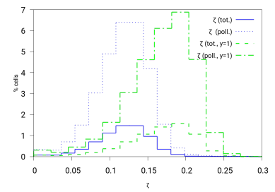
Figure 4: Percentage of cells with $\zeta$ in $\Delta>1.5$ at $t_{eq}$ (blue lines). Same case with $y=1$ is shown as green lines. The percentage is determined over the total volume (solid/dashed lines) and the polluted volume (dotted/dashed-dotted).

In conclusion, we emphasize that the possibility of using $\zeta$ as additional tracer of UVBSS fluctuations is severely limited by the number of mildly over-dense and polluted systems found in the cosmic web.

4 Conclusions

In this paper we post-process a hydrodynamic simulation which includes metal pollution with the multi-frequency cosmological radiative transfer (RT) code CRASH3 to study the amplitude and statistical relevance of spatial fluctuations of the UV background spectral shape (UVBSS) at the epoch of helium reionisation ($z\approx 3$). As the slope of the UVBSS can not be inferred by direct observations, its fluctuations must be constrained by combining the observed scatter in two quantities sensitive to the shape around the He$\,{\rm{\scriptstyle II\ }}$ ionisation potential: $\eta\equiv N_{\textrm{HeII}}/N_{\textrm{HI}}$ and $\zeta\equiv\tau_{\textrm{SiIV}}/\tau_{\textrm{CIV}}$. Note that a theoretical investigation of this problem can not be effectively performed with conventional UVB models which do not include an accurate RT. In this work, for the first time in the literature, we employ a radiative transfer approach through H, He and metal species to evaluate $\eta$ and $\zeta$ self-consistently, guaranteeing that the significant spatial fluctuations obtained are indeed due to the combined effect of metal enrichment and radiation transfer. In particular:

• we find a tight correlation of the $\eta$ parameter and over-dense systems of the cosmic web on a scale of $10h^{-1}$ cMpc and a resolution of $\approx 78$ h^-1 ckpc; these spatial fluctuations can reach values higher than $25$% in 18% of the domain and are due to RT effects through the cosmic web;

• by computing metal ions self-consistently with the RT it is possible to reproduce spatial fluctuations of $\zeta$ higher than $25$% in 34% of the metal enriched, over-dense systems with $\Delta>1.5$ (i.e. $8$% of the total volume). To be effectively used as tracer of the UVBSS, $\zeta$ requires then the presence of a statistically relevant number of polluted, over-dense systems along observed lines of sight;

• although radiative effects remain dominant, $\zeta$ depends on both UVBSS distortions and spatial fluctuations of $[\texttt{Si}/\texttt{C}]$; we have shown that their combined effects increase the domain in which $\delta\zeta>25$%.

Future studies will focus on complementary sources of UVB fluctuations, mainly associated with the variability of quasars at the epoch of helium reionisation, and will compare their statistical significance with the present findings.

References

- Agafonova et al. (2005) Agafonova I. I., Centurión M., Levshakov S. A., Molaro P., 2005, AAP, 441, 9
- Agafonova et al. (2007) Agafonova I. I., Levshakov S. A., Reimers D., Fechner C., Tytler D., Simcoe R. A., Songaila A., 2007, AAP, 461, 893
- Aguirre et al. (2004) Aguirre A., Schaye J., Kim T.-S., Theuns T., Rauch M., Sargent W. L. W., 2004, ApJ, 602, 38
- Asplund et al. (2004) Asplund M., Grevesse N., Sauval A. J., Allende Prieto C., Kiselman D., 2004, AAP, 417, 751
- Bolton et al. (2006) Bolton J. S., Haehnelt M. G., Viel M., Carswell R. F., 2006, MNRAS, 366, 1378
- Ciardi et al. (2012) Ciardi B., Bolton J. S., Maselli A., Graziani L., 2012, MNRAS, 423, 558
- Davies & Furlanetto (2014) Davies F. B., Furlanetto S. R., 2014, MNRAS, 437, 1141
- Davies et al. (2017) Davies F. B., Furlanetto S. R., Dixon K. L., 2017, MNRAS, 465, 2886
- Fan et al. (2002) Fan X., Narayanan V. K., Strauss M. A., White R. L., Becker R. H., Pentericci L., Rix H.-W., 2002, AJ, 123, 1247
- Fardal et al. (1998) Fardal M. A., Giroux M. L., Shull J. M., 1998, AJ, 115, 2206
- Fechner & Reimers (2007) Fechner C., Reimers D., 2007, AAP, 461, 847
- Ferland et al. (1998) Ferland G. J., Korista K. T., Verner D. A., Ferguson J. W., Kingdon J. B., Verner E. M., 1998, PASP, 110, 761
- Giroux & Shull (1997) Giroux M. L., Shull J. M., 1997, AJ, 113, 1505
- Graziani et al. (2013) Graziani L., Maselli A., Ciardi B., 2013, MNRAS, 431, 722
- Graziani et al. (2018) Graziani L., Ciardi B., Glatzle M., 2018, MNRAS, 479, 4320
- Grevesse & Sauval (1998) Grevesse N., Sauval A. J., 1998, SSR, 85, 161
- Haardt & Madau (1996) Haardt F., Madau P., 1996, ApJ, 461, 20
- Haardt & Madau (2012) Haardt F., Madau P., 2012, ApJ, 746, 125
- Heap et al. (2000) Heap S. R., Williger G. M., Smette A., Hubeny I., Sahu M. S., Jenkins E. B., Tripp T. M., Winkler J. N., 2000, ApJ, 534, 69
- Hogan et al. (1997) Hogan C. J., Anderson S. F., Rugers M. H., 1997, AJ, 113, 1495
- Kim et al. (2002) Kim T.-S., Cristiani S., D’Odorico S., 2002, AAP, 383, 747
- Levshakov et al. (2008) Levshakov S. A., Agafonova I. I., Reimers D., Hou J. L., Molaro P., 2008, AAP, 483, 19
- Maio et al. (2010) Maio U., Ciardi B., Dolag K., Tornatore L., Khochfar S., 2010, MNRAS, 407, 1003
- Maselli & Ferrara (2005) Maselli A., Ferrara A., 2005, MNRAS, 364, 1429
- McQuinn (2009) McQuinn M., 2009, ApJL, 704, L89
- McQuinn & Worseck (2014) McQuinn M., Worseck G., 2014, MNRAS, 440, 2406
- Meiksin (2009) Meiksin A. A., 2009, Reviews of Modern Physics, 81, 1405
- Meiksin & Tittley (2012) Meiksin A., Tittley E. R., 2012, MNRAS, 423, 7
- Miralda-Escude (1993) Miralda-Escude J., 1993, MNRAS, 262, 273
- Reimers et al. (1997) Reimers D., Kohler S., Wisotzki L., Groote D., Rodriguez-Pascual P., Wamsteker W., 1997, AAP, 327, 890
- Savaglio et al. (1997) Savaglio S., Cristiani S., D’Odorico S., Fontana A., Giallongo E., Molaro P., 1997, AAP, 318, 347
- Shull et al. (1999) Shull J. M., Roberts D., Giroux M. L., Penton S. V., Fardal M. A., 1999, AJ, 118, 1450
- Shull et al. (2004) Shull J. M., Tumlinson J., Giroux M. L., Kriss G. A., Reimers D., 2004, ApJ, 600, 570
- Shull et al. (2010) Shull J. M., France K., Danforth C. W., Smith B., Tumlinson J., 2010, ApJ, 722, 1312
- Smette et al. (2002) Smette A., Heap S. R., Williger G. M., Tripp T. M., Jenkins E. B., Songaila A., 2002, ApJ, 564, 542
- Songaila (1998) Songaila A., 1998, AJ, 115, 2184
- Songaila & Cowie (1996) Songaila A., Cowie L. L., 1996, AJ, 112, 335
- Songaila et al. (1995) Songaila A., Hu E. M., Cowie L. L., 1995, NATURE, 375, 124
- Springel (2005) Springel V., 2005, MNRAS, 364, 1105
- Syphers & Shull (2014) Syphers D., Shull J. M., 2014, ApJ, 784, 42
- Syphers et al. (2011) Syphers D., Anderson S. F., Zheng W., Meiksin A., Haggard D., Schneider D. P., York D. G., 2011, ApJ, 726, 111
- Theuns et al. (1998) Theuns T., Leonard A., Efstathiou G., Pearce F. R., Thomas P. A., 1998, MNRAS, 301, 478
- Tornatore et al. (2007) Tornatore L., Borgani S., Dolag K., Matteucci F., 2007, MNRAS, 382, 1050
- Worseck et al. (2007) Worseck G., Fechner C., Wisotzki L., Dall’Aglio A., 2007, AAP, 473, 805
- Zheng et al. (2004) Zheng W., et al., 2004, ApJ, 605, 631