Coarse-graining of overdamped Langevin dynamics via the Mori-Zwanzig formalism

Abstract.

The Mori–Zwanzig formalism is applied to derive an equation for the evolution of linear observables of the overdamped Langevin equation. To illustrate the resulting equation and its use in deriving approximate models, a particular benchmark example is studied both numerically and via a formal asymptotic expansion. The example considered demonstrates the importance of memory effects in determining the correct temporal behaviour of such systems.

1. Introduction

Molecular dynamics (MD) is a widely–used simulation technique which captures the atomistic details of material systems, allowing the prediction of their properties and behavior [48, 18]. However, despite the vast increases in computational capacity over recent decades, it is still not always possible to work with MD models at full resolution, particularly when studying large, complex systems over long time–scales. Fortunately, in many cases, the objectives of a simulation occur within a small region of interest. This observation has led to the development of coarse–grained MD (CGMD) models, in which excess degrees of freedom are incorporated implicitly [19, 50, 17, 46, 26, 28, 55, 16, 15].

Building reliable and efficient CGMD models attuned to the quantities of interest is a difficult problem. First, the simulator must find appropriate variables which capture the quantities of interest [23], often termed reaction coordinates. Once these are fixed, an appropriate proxy model for the reaction coordinates must be obtained, which implicitly incorporates the interaction between the reaction coordinates and unresolved degrees of freedom [48, 16, 36, 15, 31, 58]. If the objectives of a simulation are ‘static’ macroscopic equilibrium properties such as free energy or reaction rates, then a wide variety of choices of proxy dynamics which appropriately sample the relevant measures are available. However, if the objective is to capture a dynamical property of the physical system such as kinematic viscosity or a diffusion rate, then it is important to capture the correct effective dynamics of the reaction coordinates arising due to the relevant dynamics of the full system over moderate timescales [44, 48, 24, 18, 8, 57].

In recent years, a variety of studies of CGMD schemes have been undertaken, aiming to analyse the predictions of such schemes. In all cases, the ultimate goal is to obtain verifiable, statistically accurate predictions of the true dynamics for various applications. The wide variety of mathematical techniques used includes

• optimal prediction techniques [9, 10, 7, 20];

• information-theoretic tools [46, 4, 27, 45, 14];

• statistical filtering and ensemble methods [1, 5, 42];

• identification of an appropriate parametrization [35, 47, 22, 11];

• series expansion [53, 62, 34];

• pathwise estimates [32, 37, 29, 33]; and

• conditional expectations [30].

Here, our focus is on the Mori–Zwanzig (MZ) approach to CGMD benchmark problem [49, 64, 2, 3, 65]. The MZ formalism provides an exact expression of the dynamics for a CGMD scheme, and is governed by three terms which separate out different contributions to the true dynamics, each of which has a different statistical physical meaning. This decomposition allows a study of the sources of error: the first term accounts for a conservative dynamics due to the effective interactions between the coarse grained variables; the second is a history-dependent term determined by a time integral of a memory kernel which represents the interactions between the resolved and unresolved variables; and the third term represents the random thermal fluctuations arising from unresolved variables. In different situations, each of these terms may have a more or less important role, but to correctly capture the dynamical properties and validate an effective model, it is critical to measure the relative size and behaviour of these terms accurately.

Our study concentrates particularly on the memory term, which may heuristically be thought of as measuring the extent to which the set of reaction coordinates is decoupled from the unresolved degrees of freedom. In recent years, there have been tremendous efforts to investigate memory terms from MZ projections, for a variety of classes of dynamics, see for example [2, 9, 12, 38, 60, 23, 6, 39, 56, 59, 40, 61]. One common approach is to hope that a time-scale separation between the resolved and unresolved variables occurs, i.e. the fluctuations of the unresolved variables occur on a much faster timescale than those of the resolved variables, and therefore the two sets of variables are weakly correlated. In such cases, the memory kernel decay rapidly, approximating a delta function in time [8].

Our aim in this paper is to demonstrate that while such delta approximations of the memory kernel are appropriate in many situations, it is not generally to be expected that the memory kernel is independent of the value of the reaction coordinate, even in the simple situation where the chosen reaction coordinates are linear. To capture the correct dynamics, further careful analysis and sampling of the memory is therefore required.

As an illustration of this issue, we consider the dynamical behaviour of a gradient flow with stochastic forcing (often called the overdamped Langevin equation), demonstrating that at least in this case, a naïve approach to approximating the memory kernel yields a poor approximation of the dynamics. We hope that the benchmark problem we consider here will provide insight which will enable the study of CGMD derived from full Langevin dynamics based on reliable asymptotic analysis in future.

1.1. Outline

This paper is organized as follows. In Section 2, we review the Mori–Zwanzig formalism applied to general gradient flow systems, and in Theorem 2.1, derive an exact equation for the evolution of linear observables within an abstract framework. Our benchmark example is discussed in Section 3, and an asymptotic analysis is performed to obtain approximations of the various terms in the MZ equation. Finally, we study this particular example numerically in Section 4.

2. Formulation of the problem

As our reference fine–scale dynamical system, we consider the following overdamped Langevin dynamics defined on $\mathbb{R}^{N}$:

$$d\mathbf{X}_{t}=-\nabla_{\mathbf{x}}V(\mathbf{X}_{t})dt+\sqrt{2\beta^{-1}}d\mathbf{B}_{t}.$$ (2.1)

Here, $\mathbf{B}_{t}$ denotes a standard vector–valued Brownian motion, $V(\cdot)$ is a potential energy and $\beta$ is the inverse temperature. Throughout this work, we assume that $V$ is at least of class $C^{2}$, and satisfies the following conditions:

1. There exist constants $\gamma>0$ and $\delta\geq 0$ and $R>0$ such that

   $$-\nabla V(\mathbf{x})\cdot\mathbf{x}\leq\gamma|\mathbf{x}|^{2}+\delta\qquad\text{for all }|\mathbf{x}|\geq R.$$

2. The gradient $\nabla V(\mathbf{x})$ is globally Lipschitz, i.e. there exists $\alpha>0$ such that

   $$\big{|}\nabla V(\mathbf{x})-\nabla V(\mathbf{y})\big{|}\leq\alpha\,|\mathbf{x}-\mathbf{y}|.$$

Under condition (1), it is well–known [54] that the dynamics defined by (2.1) are ergodic with respect to the Gibbs measure, $\mu$, given by $d\mu(\mathbf{x})=\frac{1}{Z}e^{-\beta V(\mathbf{x})}d\mathbf{x}$ where $Z$ is the partition function

$$Z:=\int e^{-\beta V(\mathbf{x})}d\mathbf{x}.$$

Given a regular function $\mathbf{F}:\mathbb{R}^{N}\rightarrow\mathbb{R}^{m}$, which may be thought of as describing a family of reaction coordinates, we may apply Itô’s formula to deduce that the value of $\mathbf{F}(\mathbf{X}_{t})$ is governed by the Itô SDE

$$d\mathbf{F}(\mathbf{X}_{t})=\Big{(}-\nabla V(\mathbf{X}_{t})\cdot\nabla\mathbf{F}(\mathbf{X}_{t})+\beta^{-1}\Delta\mathbf{F}(\mathbf{X}_{t})\Big{)}dt+\sqrt{2\beta^{-1}}\nabla\mathbf{F}(\mathbf{X}_{t})\cdot d\mathbf{B}_{t}.$$ (2.2)

In particular, if we consider a linear coarse–graining selector $\mathbf{F}(\mathbf{x}):=\Phi\mathbf{x}$, where $\Phi\in\mathbb{R}^{m\times N}$ is a constant matrix, (2.2) becomes

$$d\mathbf{F}(\mathbf{X}_{t})=-\Phi\nabla V(\mathbf{X}_{t})dt+\sqrt{2\beta^{-1}}\Phi\,d\mathbf{B}_{t}.$$ (2.3)

Such linear coordinates are commonly used in CGMD schemes, particularly for large molecules such as polymers [17, 13, 52]. If we are interested in the value of the reaction coordinates described by $\mathbf{F}$ alone, then (2.3) provides an equation for their evolution. In general however, since the first term on the right–hand side of the equation depends on the full process $\mathbf{X}_{t}$, this is not a closed equation for the value of $\mathbf{F}(\mathbf{X}_{t})$.

In order to formulate a closed approximate equation for $\mathbf{F}(\mathbf{X}_{t})$, we use the Mori–Zwanzig formalism, which uses projection operators to decompose the equations describing observables of a dynamical system into terms involving the value of the observables alone, and ‘error’ terms describing the contribution of variations of $\mathbf{X}_{t}$ which do not directly change the value of the observable.

In this case, the projection operator we choose to apply is the Zwanzig projection, which involves taking a conditional expectation with respect to the Gibbs distribution, i.e.

$$\mathcal{P}\mathbf{g}=\mathbb{E}_{\mu}\big{[}\mathbf{g}\,\big{|}\,\mathbf{F}(\mathbf{x})=\mathbf{h}\big{]}:=\frac{\int_{\mathbf{F}^{-1}(\mathbf{h})}\mathbf{g}(\mathbf{x})\,e^{-\beta V(\mathbf{x})}d\mathbf{x}}{\int_{\mathbf{F}^{-1}(\mathbf{h})}e^{-\beta V(\mathbf{x})}d\mathbf{x}};$$ (2.4)

note that in the above formula, we have cancelled the common factor $\frac{1}{Z}$ from the numerator and denominator. It may be verified that $\mathcal{P}$ is an orthogonal projection on the space of square–integrable observables, i.e. $L^{2}(\mathbb{R}^{N};e^{-\beta V(\mathbf{x})}d\mathbf{x})$, and we can therefore define its orthogonal counterpart,

$$\mathcal{Q}:=\mathcal{I}-\mathcal{P}.$$

In particular, we note that the evolution of (2.3) can be divided into the stationary, mean–zero process induced by the Brownian motion, and the evolution of the mean value of $\mathbf{F}(\mathbf{X}_{t})$. To consider the behaviour of the latter quantity given knowledge of $\mathbf{X}_{0}$, we define

$$\mathbf{h}_{t}(\mathbf{x})=\mathbb{E}\big{[}\mathbf{F}(\mathbf{X}_{t})\,\big{|}\,\mathbf{X}_{0}=\mathbf{x}].$$ (2.5)

The evolution of this quantity is governed by the usual generator of the SDE (2.1),

$$\mathcal{L}:=-\nabla V\cdot\nabla+\beta^{-1}\Delta.$$ (2.6)

Using this definition, the Feynmann–Kac formula governing the evolution of $\mathbf{h}$ states that the function $\mathbf{h}$ solves the PDE

$$\partial_{t}\mathbf{h}_{t}=\mathcal{L}\mathbf{h}_{t}\qquad\text{with}\qquad\mathbf{h}_{0}=\mathbf{F}.$$ (2.7)

Using the definition of $\mathcal{P}$, we apply the Mori–Zwanzig formalism to provide a different expression of (2.7), stated in the following theorem.

Theorem 2.1.

Let $\mathbf{X}_{t}$ satisfy the SDE on $\mathbb{R}^{N}$

$$d\mathbf{X}_{t}=-\nabla V(\mathbf{X}_{t})dt+\sqrt{2\beta^{-1}}d\mathbf{B}_{t},$$

and given a constant matrix of full rank $\Phi\in\mathbb{R}^{N\times m}$, the observable

$$\mathbf{h}_{t}(\mathbf{x})=\mathbb{E}\big{[}\mathbf{F}(\mathbf{X}_{t})\,\big{|}\,\mathbf{X}_{0}=\mathbf{x}];$$ (2.8)

satisfies the following integro–differential equation:

$$\partial_{t}\mathbf{h}_{t}(\mathbf{x})=-\Phi\Phi^{T}\,\nabla\mathcal{S}\big{(}\mathbf{h}_{t}(\mathbf{x})\big{)}+\int_{0}^{t}\mathcal{M}_{s}\big{(}\mathbf{h}_{t-s}(\mathbf{x})\big{)}\cdot\nabla\mathcal{S}\big{(}\mathbf{h}_{t-s}(\mathbf{x})\big{)}-\frac{1}{\beta}\mathsf{div}\,\mathcal{M}_{s}\big{(}\mathbf{h}_{t-s}(\mathbf{x})\big{)}ds+\mathcal{F}_{t}(\mathbf{x}),$$ (2.9)

where:

1. $\mathcal{S}:\mathbb{R}^{m}\to\mathbb{R}$ is the effective potential, defined to be

   $$\mathcal{S}(\mathbf{h}):=-\frac{1}{\beta}\log Z_{\Phi}(\mathbf{h})\text{ with }Z_{\Phi}(\mathbf{h}):=\int_{\mathbf{F}^{-1}(\mathbf{h})}e^{-\beta V(\mathbf{x})}d\mathbf{x},$$ (2.10)

2. $\mathcal{M}_{s}:\mathbb{R}^{m}\to\mathbb{R}^{m\times m}$ is the memory kernel, defined to be

   $$\mathcal{M}_{s}(\mathbf{h}):=\beta\,\mathbb{E}\big{[}e^{s\mathcal{Q}\mathcal{L}}\mathcal{Q}\mathcal{L}\mathbf{F}\otimes\mathcal{Q}\mathcal{L}\mathbf{F}\,\big{|}\,\mathbf{F}(\mathbf{x})=\mathbf{h}\big{]}=\beta\,\mathbb{E}\big{[}\mathcal{F}_{s}\otimes\mathcal{F}_{0}\,\big{|}\,\mathbf{F}(\mathbf{x})=\mathbf{h}\big{]},$$ (2.11)

3. and $\mathcal{F}_{t}:\mathbb{R}^{N}\to\mathbb{R}$ is the fluctuating force, defined to be

   $$\mathcal{F}_{t}:=e^{t\mathcal{Q}\mathcal{L}}\mathcal{Q}\mathcal{L}\mathbf{F}.$$ (2.12)

A proof of this result is given in Appendix A, and involves adapting standard variants of the Mori–Zwanzig formalism already present in the literature to this stochastic setting.

Remark 2.1.

The Mori–Zwanzig formalism [63, 49, 64, 51] uses projection operators to rewrite the equations governing observables of a dynamical system. Various formulations have been developed in recent years with a variety of applications in mind, and influence our own derivation, including: [38] treating crystalline solids via the harmonic approximation; [62] for the harmonic oscillators based on operator series expansions of the orthogonal dynamics propagator; [43] for the full Langevin dynamics model based on reduced-order modeling; [25] for a model based on dissipative particle dynamics; and [52] for a ‘hybrid’ coarse–graining map of a Hamiltonian model.

Recombining the evolution of the mean $\mathbf{h}_{t}$ given by (2.9) and adding back the Brownian motion, we find that (2.3) can be written

$$d\mathbf{F}(\mathbf{X}_{t}) =-\Phi\Phi^{T}\,\nabla\mathcal{S}\big{(}\mathbf{F}(\mathbf{X}_{t})\big{)}dt+\int_{0}^{t}\mathcal{M}_{s}\big{(}\mathbf{F}(\mathbf{X}_{t-s})\big{)}\cdot\nabla\mathcal{S}\big{(}\mathbf{F}(\mathbf{X}_{t-s})\big{)}ds\,dt$$ (2.13)

$$\hskip 56.9055pt-\int_{0}^{t}\frac{1}{\beta}\mathsf{div}\,\mathcal{M}_{s}\big{(}\mathbf{F}(\mathbf{X}_{t-s})\big{)}ds\,dt+d\mathcal{F}_{t}+\sqrt{2\beta^{-1}}\Phi d\mathbf{B}_{t}.$$

It is important to note at this point that (2.13) is equivalent to considering the full evolution (2.3), in particular because $\mathcal{F}_{t}$ is unknown. Equation (2.13) therefore remains unclosed; however, the power of this formulation is that if $\mathcal{F}_{t}$ has statistics which are well–captured by some proxy process $\widetilde{\mathcal{F}}_{t}$, and $\mathcal{S}$ is either known or accurately approximated, then we can obtain a closed–form approximate dynamics

$$d\mathbf{h}_{t}=-\Phi\Phi^{T}\nabla\mathcal{S}(\mathbf{h}_{t})dt+\bigg{(}\int_{0}^{t}\widetilde{\mathcal{M}}_{s}(\mathbf{h}_{t-s})\nabla\mathcal{S}(\mathbf{h}_{t-s})-\frac{1}{\beta}\mathsf{div}\,\widetilde{\mathcal{M}}_{s}(\mathbf{h}_{t-s})ds\bigg{)}\,dt\\ +d\widetilde{\mathcal{F}}_{t}+\sqrt{2\beta^{-1}}\Phi d\mathbf{B}_{t},$$

where $\widetilde{\mathcal{M}}_{s}(\mathbf{h})$ is the autocovariance function of $\widetilde{\mathcal{F}}_{t}(\mathbf{h})$ (see for example [41]).

To explore this formulation and better understand the relationship between the terms involved, the remainder of the paper is devoted to an exploration of a dynamics where an accurate approximation (2.9) and the terms within it.

3. A benchmark problem

In this section, we will consider the overdamped Langevin equation (2.1) in the particular case where $\mathbf{x}\in\mathbb{R}^{2}$, and the potential energy is defined to be

$$V(x,y):=\frac{\mu}{2}x^{2}+\frac{\lambda}{2}\big{(}\tau\sin(\omega x)-y\big{)}^{2}$$ (3.1)

with $\mu$, $\lambda$, $\tau$, $\omega\geq 0$ being parameters. Specifying even further, we will focus on the case where $\lambda\gg\mu$, so that there is a separation between the timescale of relaxation for the $x$ and $y$ variables. As such, $x$ is a ‘slow’ variable, and is a natural candidate for a reaction coordinate of the system; as in Section 2, we therefore consider

$$\mathbf{F}(\mathbf{x})=\Phi\mathbf{x}\qquad\text{where}\qquad\Phi:=\left(\begin{array}[]{cc}1&0\end{array}\right).$$

The second term in (3.1), i.e. $\frac{\lambda}{2}\big{(}\tau\sin(\omega x)-y\big{)}^{2}$, has been chosen to emulate a form of free energy barrier to the dynamics, since when $\tau\sim 1$, $\omega\gg 1$ and $\beta\gg 1$, we expect trajectories of the dynamics to remain close to the manifold $y=\sin(\omega x)$; see Figure 1 for representations of different energy landscapes.

(a) $\mu=2,\lambda=20,\omega=10,\tau=2$

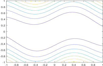
(b) $\mu=2,\lambda=20,\omega=4,\tau=0.2$

Figure 1. Contour plots of the potential energy $V(x,y)$ defined in (3.1): $\lambda/\mu\gg 1$ and $\omega\tau$ is chosen to be $\gg 1$ for figure (a) and $<1$ for figure (b), respectively.

As a consequence, we expect that as $\tau$ and $\omega$ increase with $\frac{\lambda}{\mu}\gg 1$, the dynamics should to take progressively longer to approach a fixed neighbourhood of the global equilibrium at $0$ from a generic initial condition, since the dynamics must effectively ‘travel further’ along the meandering valley in the potential to get there.

3.1. Derivation of approximate dynamics

Under the assumptions described above, we compute $\mathcal{P}\mathcal{L}\mathbf{F}$ and $\mathcal{Q}\mathcal{L}\mathbf{F}$, and use these to derive approximations of the terms involved in (2.9).

1. Computation of $\mathcal{P}\mathcal{L}\mathbf{F}$. The effective potential $\mathcal{S}(x)$ defined in (2.10) is equal to

   $$\begin{split}\mathcal{S}(x)=&-\frac{1}{\beta}\log\left(\int_{\mathbb{R}}e^{-\beta V(x,y)}dy\right)=\frac{\mu}{2}x^{2}+\mathsf{const},\end{split}$$ (3.2)

   as the unresolved variable $y$ follows normal distribution $y\sim N(\tau\sin(\omega x),\frac{1}{\beta\lambda})$, and hence

   $$\mathcal{P}\mathcal{L}\mathbf{F}=\left(\begin{array}[]{c}-\mu x\\ 0\end{array}\right).$$ (3.3)

2. Computation of $\mathcal{Q}\mathcal{L}\mathbf{F}$. Clearly $\mathcal{Q}\mathcal{L}\mathbf{F}=\mathcal{L}\mathbf{F}-\mathcal{P}\mathcal{L}\mathbf{F}$, so using (3.3), we have

   $$\mathcal{Q}\mathcal{L}\mathbf{F}=\mathcal{Q}\mathcal{L}\left(\begin{array}[]{c}x\\ y\end{array}\right)=\left(\begin{array}[]{c}-\lambda\tau\omega\left(\tau\sin(\omega x)-y\right)\,\cos(\omega x)\\ -\lambda\left(y-\tau\sin(\omega x)\right)\end{array}\right).$$

3. Approximation of $\mathcal{M}_{s}$. Recalling the definition of the memory function $\mathcal{M}_{s}(\mathbf{F})$ from (2.11), we must compute or otherwise approximate the expression $\mathcal{Q}\mathcal{L}e^{s\mathcal{Q}\mathcal{L}}\mathbf{F}\otimes\mathcal{Q}\mathcal{L}\mathbf{F}$. To do so, we define characteristic curves of the orthogonal dynamics, $\widetilde{\mathbf{x}}_{s}=(\widetilde{x}_{s},\widetilde{y}_{s})=e^{s\mathcal{Q}\mathcal{L}}\widetilde{\mathbf{x}}_{0}$, and find that

   $$\begin{split}&\mathcal{Q}\mathcal{L}e^{s\mathcal{Q}\mathcal{L}}\mathbf{F}(\widetilde{\mathbf{x}}_{0})\otimes\mathcal{Q}\mathcal{L}\mathbf{F}(\widetilde{\mathbf{x}}_{0})=\Phi\dot{\widetilde{\mathbf{x}}}_{s}\otimes\Phi\dot{\widetilde{\mathbf{x}}}_{0}\\ &\qquad=\lambda^{2}\tau^{2}\omega^{2}\left(\tau\sin(\omega\widetilde{x}_{s})-\widetilde{y}_{s}\right)\cos(\omega\widetilde{x}_{s})\cdot\,\left(\tau\sin(\omega\widetilde{x}_{0})-\widetilde{y}_{0}\right)\cos(\omega\widetilde{x}_{0}).\end{split}$$ (3.4)

   We now change variable with the intention of linearizing, setting $\widetilde{u}_{s}:=\widetilde{x}_{s}-\widetilde{x}_{0}$ and $\widetilde{v}_{s}:=\widetilde{y}_{s}-\tau\sin(\omega\widetilde{x}_{0})$. Expressed in these new variables, the action of the orthogonal dynamics is equivalent to solving the ODE system

   $$\left(\begin{array}[]{c}\dot{\widetilde{u}}_{s}\\ \dot{\widetilde{v}}_{s}\end{array}\right) =\left(\begin{array}[]{c}-\lambda\tau\omega\left(\tau\sin(\omega(\widetilde{x}_{0}+\widetilde{u}_{s}))-\tau\sin(\omega\widetilde{x}_{0})-\widetilde{v}_{s}\right)\,\cos\big{(}\omega(\widetilde{x}_{0}+\widetilde{u}_{s})\big{)}\\ -\lambda\left(\tau\sin(\omega\widetilde{x}_{0})+\widetilde{v}_{s}-\tau\sin\big{(}\omega(\widetilde{x}_{0}+\widetilde{u}_{s})\big{)}\right)\end{array}\right).$$

   Since we have assumed that $\lambda\gg\mu$, given knowledge of $\widetilde{x}_{0}$ alone, we expect that initial conditions for the orthogonal dynamics to be concentrated near $(\widetilde{x}_{0},\widetilde{y}_{0})=(\widetilde{x}_{0},\tau\sin(\omega\widetilde{x}_{0}))$, and so linearising on this basis, we obtain

   $$\left(\begin{array}[]{c}\dot{\widetilde{u}}_{s}\\ \dot{\widetilde{v}}_{s}\end{array}\right)=\lambda\left(\begin{array}[]{cc}-\tau^{2}\omega^{2}\cos^{2}(\omega\widetilde{x}_{0})&\tau\omega\cos(\omega\widetilde{x}_{0})\\ \tau\omega\cos(\omega\widetilde{x}_{0})&-1\end{array}\right)\left(\begin{array}[]{c}\widetilde{u}_{s}\\ \widetilde{v}_{s}\end{array}\right)+\mathcal{O}(\widetilde{u}_{s}^{2},\widetilde{v}_{s}^{2},\widetilde{u}_{s}\widetilde{v}_{s}).$$ (3.5)

   Noting in particular that $\widetilde{u}_{0}=0$ since $\widetilde{u}_{s}=\widetilde{x}_{s}-\widetilde{x}_{0}$, and neglecting higher–order terms in (3.5), the solution is approximately

   $$\left(\begin{array}[]{c}\widetilde{u}_{s}\\ \widetilde{v}_{s}\end{array}\right) \approx\frac{1}{1+\tau^{2}\omega^{2}\cos^{2}(\omega\widetilde{x}_{0})}\left(\begin{array}[]{c}\widetilde{v}_{0}\tau\omega\cos(\omega\widetilde{x}_{0})\\ \widetilde{v}_{0}\tau^{2}\omega^{2}\cos^{2}(\omega\widetilde{x}_{0})\end{array}\right)$$

   $$\qquad\qquad+\frac{e^{-\lambda\big{(}1+\tau^{2}\omega^{2}\cos^{2}(\omega\widetilde{x}_{0})\big{)}s}}{1+\tau^{2}\omega^{2}\cos^{2}(\omega\widetilde{x}_{0})}\left(\begin{array}[]{c}-\widetilde{v}_{0}\tau\omega\cos(\omega\widetilde{x}_{0})\\ \widetilde{v}_{0}\end{array}\right),$$

   and therefore

   $$\dot{\widetilde{x}}_{s}=\dot{\widetilde{u}}_{s}\approx\lambda\tau\omega\widetilde{v}_{0}\cos(\omega\widetilde{x}_{0})e^{-\lambda\big{(}1+\tau^{2}\omega^{2}\cos^{2}(\omega\widetilde{x}_{0})\big{)}s}.$$ (3.6)

   When conditioning on knowledge of $\widetilde{x}_{0}$, it follows that $\widetilde{y}_{0}\sim\mathcal{N}(\tau\sin(\omega\widetilde{x}_{0}),\frac{1}{\lambda\beta})$, and therefore $\widetilde{v}_{0}\sim\mathcal{N}(0,\frac{1}{\lambda\beta})$: the memory kernel is therefore approximately

   $$\mathcal{M}_{s}(\mathbf{h}) =\beta\,\mathbb{E}[\mathcal{Q}\mathcal{L}e^{s\mathcal{Q}\mathcal{L}}\mathbf{F}\otimes\mathcal{Q}\mathcal{L}\mathbf{F}\,|\,\mathbf{F}(\mathbf{x})=\mathbf{h}]$$ (3.7)

   $$\approx\beta\int_{\mathbb{R}}\dot{\widetilde{u}}_{s}(\mathbf{h},\widetilde{y}_{0})\otimes\dot{\widetilde{u}}_{0}(\mathbf{h},\widetilde{y}_{0})e^{-\beta\lambda\left(\widetilde{y}_{0}-\tau\sin(\omega\mathbf{h})\right)^{2}}d\widetilde{y}_{0}$$

   $$=\lambda\tau^{2}\omega^{2}\cos^{2}(\omega\mathbf{h})e^{-\lambda\big{(}1+\tau^{2}\omega^{2}\cos^{2}(\omega\mathbf{h})\big{)}s},$$

   where in the above formula, $\dot{\widetilde{u}}_{0}=\lim_{s\to 0+}\dot{\widetilde{u}}_{s}$. Recalling the form of (2.9), we note that we must also approximate the divergence of $\mathcal{M}_{s}$; using the expression derived in (3.7), in this case we obtain

   $$\mathsf{div}\mathcal{M}_{s}(\mathbf{h})\approx-\lambda\tau^{2}\omega^{3}\sin(2\omega\mathbf{h})\left(1-\lambda\tau^{2}\omega^{2}\cos^{2}(\omega\mathbf{h})s\right)e^{-\lambda\big{(}1+\tau^{2}\omega^{2}\cos^{2}(\omega\mathbf{h})\big{)}s}.$$ (3.8)

4. Approximation of memory integral. Our next step is to approximate the first integral term involving the memory kernel in (2.9). Noting the form of (3.7), we see that this is an integral of exponential type, and therefore we apply the method of steepest descents to derive an approximation.

   We note that the exponential term in the approximate expressions (3.7) and (3.8) are maximal when $s=0$; if $\mathbf{h}_{t-s}\approx\mathbf{h}_{t}$ for small $s$, we obtain

   $$\int_{0}^{t}\mathcal{M}_{s}(\mathbf{h}_{t-s})\cdot\nabla\mathcal{S}(\mathbf{h}_{t-s})ds \approx\int_{0}^{t}\lambda\tau^{2}\omega^{2}\cos^{2}(\omega\mathbf{h}_{t-s})\,\mu\mathbf{h}_{t-s}e^{-\lambda(1+\tau^{2}\omega^{2}\cos^{2}(\omega\mathbf{h}_{t-s}))s}ds$$

   $$\approx\int_{0}^{\infty}\lambda\tau^{2}\omega^{2}\cos^{2}(\omega\mathbf{h}_{t})\,\mu\mathbf{h}_{t}e^{-\lambda(1+\tau^{2}\omega^{2}\cos^{2}(\omega\mathbf{h}_{t}))s}ds$$

   $$\approx\frac{\tau^{2}\omega^{2}\cos^{2}(\omega\mathbf{h}_{t})}{1+\tau^{2}\omega^{2}\cos^{2}(\omega\mathbf{h}_{t})}\mu\mathbf{h}_{t},$$

   and via a similar approximation for the divergence term, we have

   $$\int_{0}^{t}-\frac{1}{\beta}\mathsf{div}\left(\mathcal{M}_{s}(\mathbf{h}_{t-s})\right)ds$$

   $$\qquad\approx\int_{0}^{t}\frac{1}{\beta}\lambda\tau^{2}\omega^{3}\sin(2\omega\mathbf{h}_{t-s})\left(1-\lambda\tau^{2}\omega^{2}\cos^{2}(\omega\mathbf{h}_{t-s})s\right)e^{-\lambda(1+\tau^{2}\omega^{2}\cos^{2}(\omega\mathbf{h}_{t-s}))s}ds$$

   $$\qquad\approx\int_{0}^{\infty}\frac{1}{\beta}\lambda\tau^{2}\omega^{3}\sin(2\omega\mathbf{h}_{t})\left(1-\lambda\tau^{2}\omega^{2}\cos^{2}(\omega\mathbf{h}_{t})s\right)e^{-\lambda(1+\tau^{2}\omega^{2}\cos^{2}(\omega\mathbf{h}_{t}))s}ds$$

   $$\qquad\approx\frac{1}{\beta}\frac{\tau^{2}\omega^{3}\sin(2\omega\mathbf{h}_{t})}{(1+\tau^{2}\omega^{2}\cos^{2}(\omega\mathbf{h}_{t}))^{2}}.$$

   Combining these approximations, we obtain an approximation of the memory contributions in (2.9) as

   $$\begin{split}&\int_{0}^{t}\mathcal{M}_{s}(\mathbf{h}_{t-s})\cdot\nabla\mathcal{S}(\mathbf{h}_{t-s})-\frac{1}{\beta}\mathsf{div}\,\mathcal{M}_{s}(\mathbf{h}_{t-s})ds\\ &\qquad\qquad\approx\frac{\tau^{2}\omega^{2}\cos^{2}(\omega\mathbf{h}_{t})}{1+\tau^{2}\omega^{2}\cos^{2}(\omega\mathbf{h}_{t})}\mu\mathbf{h}_{t}+\frac{1}{\beta}\frac{\tau^{2}\omega^{3}\sin(2\omega\mathbf{h}_{t})}{(1+\tau^{2}\omega^{2}\cos^{2}(\omega\mathbf{h}_{t}))^{2}}.\end{split}$$ (3.9)

   Notably, if $\tau\sim 1$, the second term is negligible compared with the first both when $\omega\ll 1$, and when $\omega\gg 1$. We will therefore discard the latter term in these cases.

5. Fluctuating force. Above, we have shown that the memory kernel can be approximated as

   $$\mathcal{M}_{s}(\mathbf{h})\approx\frac{\tau^{2}\omega^{2}\cos^{2}(\omega\mathbf{h})}{1+\tau^{2}\omega^{2}\cos^{2}(\omega\mathbf{h})}\delta_{0}(s).$$

   Since $\mathcal{M}_{s}$ is the autocovariance of $\mathcal{F}_{t}$ multiplied by $\beta$, and the autocovariance of the white noise already present is $\beta^{-1}\delta_{0}(s)$, it is natural, in view of the Fluctuation–Dissipation Theorem, to define a new stochastic forcing which has an autocovariance that is the sum of these two contributions, i.e.

   $$d\mathcal{F}_{t}+\sqrt{2\beta^{-1}}d\mathbf{B}_{t}\approx\sqrt{\frac{2\beta^{-1}}{1+\tau^{2}\omega^{2}\cos^{2}(\omega\mathbf{h})}}d\mathbf{B}_{t}$$

Combining the approximations above, in the case where $\omega\gg 1$, we obtain the closed–form approximate equation

$$d\mathbf{h}_{t}=-\frac{\mu\mathbf{h}_{t}}{1+\tau^{2}\omega^{2}\cos^{2}(\omega\mathbf{h}_{t})}dt+\sqrt{\frac{2\beta^{-1}}{1+\tau^{2}\omega^{2}\cos^{2}(\omega\mathbf{h}_{t})}}d\mathbf{B}_{t}$$ (3.10)

Notably, the drift term in this equation is independent of $\beta$.

3.2. Other choices of approximate dynamics

The derivation of the effective dynamics (3.9) was informed by the Mori–Zwanzig formalism, but other choices could be made, and may be more appropriate in other circumstances.

1. Discarding memory and fluctuating force. In [30], the authors consider another choice of effective dynamics, which in our setting, amounts to considering

   $$d\boldsymbol{\xi}_{t}=-\Phi\Phi^{T}\nabla\mathcal{S}(\boldsymbol{\xi}_{t})dt+\sqrt{2\beta^{-1}\Phi\Phi^{T}}d\mathbf{B}_{t}.$$ (3.11)

   This is equivalent to (2.13) where the memory and fluctuating force terms have been neglected entirely. For the evolution of the mean $\mathbf{h}_{t}$, this choice of dynamics yields

   $$\partial_{t}\mathbf{h}_{t}=-\Phi\Phi^{T}\nabla\mathcal{S}(\mathbf{h}_{t})dt$$ (3.12)

   as the effective equation for the observable we consider. The authors have proved error bounds on the time marginals of the resulting probability distribution when compared the true dynamics captured by (2.3); applying [30, Proposition 3.1] to our case gives the bound

   $$H(\psi_{t}|\phi_{t})\leq\frac{\beta\tau^{2}\omega^{2}}{4}\left[H\left(\psi_{0}\middle|\mu\right)-H\left(\psi_{t}\middle|\mu\right)\right],$$ (3.13)

   where:

   1. $H(\mu|\nu)$ is the relative entropy of a measure $\mu$ with respect to $\nu$, i.e.

      $$H(\mu|\nu):=\int\log\left(\frac{d\mu}{d\nu}\right)d\mu;$$

   2. $\mu$ is the Gibbs measure;

   3. $\psi_{t}$ is the distribution of the ‘true’ dynamics at time $t$; and

   4. $\phi_{t}$ is the distribution of solutions to (3.11) at time $t$.

   Clearly, the constant in (3.13) is large when $\tau\omega\gg 1$; this reflects the fact that neglecting the memory in this case is not sufficient to accurately capture the dynamical properties of the system, and a more sophisticated approach is needed.

2. A more naïve memory approximation. To highlight the need to conduct dynamical sampling to approximate $\mathcal{M}_{s}$ correctly, we remark that the approximation of the memory terms obtained in (3.9) is notably not the same as simply choosing to approximate

   $$\mathcal{M}_{s}(\mathbf{h}) \approx\widetilde{\mathcal{M}}_{s}(\mathbf{h}):=\beta\,\mathbb{E}[\mathcal{Q}\mathcal{L}\mathbf{x}\otimes\mathcal{Q}\mathcal{L}\mathbf{x}\,|\,\mathbf{F}(\mathbf{x})=\mathbf{h}]\,\delta_{0}(s),$$

   $$=\left(\sqrt{\frac{\lambda\beta}{2\pi}}\int\beta\,\lambda^{2}\tau^{2}\omega^{2}(\tau\sin(\omega\mathbf{h})-y)^{2}\cos^{2}(\omega\mathbf{h})e^{-\frac{1}{2}\beta\lambda(\tau\sin(\omega\mathbf{h})-y)^{2}}dy\right)\,\delta_{0}(s)$$

   $$=\lambda\tau^{2}\omega^{2}\cos^{2}(\omega\mathbf{h})\delta_{0}(s).$$

   Using $\widetilde{\mathcal{M}}_{s}$ would result in the approximate dynamics

   $$\begin{split}\partial_{t}\mathbf{h}_{t}&=\big{(}\lambda\tau^{2}\omega^{2}\cos^{2}(\omega\mathbf{h}_{t})-1\big{)}\mu\mathbf{h}_{t}+\frac{\lambda}{\beta}\tau^{2}\omega^{3}\sin(2\omega\mathbf{h}_{t}).\end{split}$$ (3.14)

   Since we have chosen $\lambda\gg 1$, we see that this approximation will yield qualitatively different dynamics to both the true dynamics for $\mathbf{F}$, (2.3), and the approximate dynamics given by (3.9); we investigate this numerically in Section 4.

The remarks above suggests that in general, careful dynamical sampling of the memory kernel is required to accurately capture the interaction between chosen reaction coordinates and the neglected degrees of freedom.

4. Numerical simulations

In this section, we conduct a numerical study of the various choices of approximate effective dynamics for the observable in the toy example considered in Section 3.1. In particular, we inspect the validity of some of the approximations made, and compare the different choices of effective dynamics described in Section 3.

4.1. Investigation of the memory kernel

The derivation of the effective dynamics for $\mathbf{h}_{t}$ made in Section 3.1 relies crucially upon a series of approximations to the memory integral in (2.9); we therefore first consider the validity of these assumptions.

1. Sampling of the memory kernel. To understand the error committed by using the approximation of the memory kernel given in (3.7), we computed the memory kernel by statistically sampling trajectories of the orthogonal dynamics. The result of this simulation for 2 different cases when $\tau\omega$ is of different sizes are shown in Figure 3. The empirical memory exhibits monotone decay in time for all values of $x_{0}$ considered, and decay is more rapid when $\tau\omega$ is large, in agreement with (3.7).

   

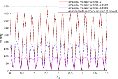
   (a) $\omega=10$, $\tau=2$

   

   (b) $\omega=4$, $\tau=.2$

   Figure 2. Comparison of empirical memory kernel and approximate form given in (3.7). In both cases $\lambda=20$ and $\mu=2$.

   

   (a) $|\cos(\omega x_{0})|=1$

   

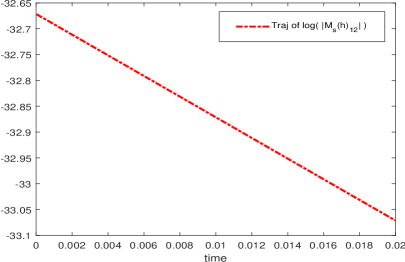
   (b) $\cos(\omega x_{0})=0$

   Figure 3. Average trajectories of $\log\left|\mathbf{M}_{s}(\mathbf{h})_{12}\right|$ under different initial condition of $x_{0}$ (see (4.1)) based on a sample of 2000 initial conditions of $y_{0}$. Initial conditions of $y_{0}$ satisfy $y_{0}\sim\mathcal{N}(\tau\sin(\omega x_{0}),\frac{1}{\beta\lambda})$, and parameters of $V$ are $\lambda=20$, $\mu=2$, $\tau=2$ and $\omega=10$.

2. The memory kernel and choice of reaction coordinate. In practice, it is impractical to compute and then integrate over long trajectories of the memory term, so a good coarse-graining selector should lead to a fast decay of the memory kernel [23].

   With this in mind, in general we set $\Sigma=\sqrt{\Phi\Phi^{T}}$, and consider

   $$\mathbf{M}_{s}(\mathbf{h}) :=\beta\mathbb{E}\big{[}e^{s\mathcal{Q}\mathcal{L}}\mathcal{Q}\mathcal{L}\mathbf{x}\otimes\mathcal{Q}\mathcal{L}\mathbf{x}\,\big{|}\,\Phi\mathbf{x}=\mathbf{h}\big{]}$$ (4.1)

   $$=\beta\mathbb{E}\left[\left(\begin{array}[]{cc}e^{s\mathcal{Q}\mathcal{L}}\mathcal{Q}\mathcal{L}\Sigma^{-1}\Phi\mathbf{x}\otimes\mathcal{Q}\mathcal{L}\Sigma^{-1}\Phi\mathbf{x}&e^{s\mathcal{Q}\mathcal{L}}\mathcal{Q}\mathcal{L}\Sigma^{-1}\Phi\mathbf{x}\otimes\mathcal{Q}\mathcal{L}\Psi\mathbf{x}\\ e^{s\mathcal{Q}\mathcal{L}}\mathcal{Q}\mathcal{L}\Psi\mathbf{x}\otimes\mathcal{Q}\mathcal{L}\Sigma^{-1}\Phi\mathbf{x}&e^{s\mathcal{Q}\mathcal{L}}\mathcal{Q}\mathcal{L}\Psi\mathbf{x}\otimes\mathcal{Q}\mathcal{L}\Psi\mathbf{x}\end{array}\right)\,\middle|\,\Phi\mathbf{x}=\mathbf{h}\right]$$

   $$=\left(\begin{array}[]{cc}\mathbf{M}_{s}(\mathbf{h})_{11}&\mathbf{M}_{s}(\mathbf{h})_{12}\\ \mathbf{M}_{s}(\mathbf{h})_{21}&\mathbf{M}_{s}(\mathbf{h})_{22}\end{array}\right).$$

   We see that $\mathbf{M}_{s}(\mathbf{h})_{11}=\Sigma^{-1}\mathcal{M}_{s}(\mathbf{h})\Sigma^{-1}$, recalling the definition of $\mathcal{M}_{S}$ from (2.11). We also note that if dynamical sampling of the orthogonal dynamics is used to approximate $\mathcal{M}_{s}$ in practice, all of the information needed to compute $\mathbf{M}_{s}$ is available.

   Intuitively, the off–diagonal blocks of $\mathbf{M}_{s}$ describe the correlation between the action of the fluctuating force on the reaction coordinates and orthogonal variables, and in particular, $\mathbf{M}_{s}(\mathbf{h})_{12}$ describes the influence of the unknown variables $\Psi\mathbf{x}$ at the current time on the dynamics of $\Phi\mathbf{x}$ at later times. We can therefore test the strength of the ‘coupling’ between the reaction coordinates and the other degrees of freedom by considering the magnitude of $\mathbf{M}_{s}(\mathbf{h})_{12}$; a log plot is shown in Figure 3 demonstrating very rapid decay of the corresponding entry.

   We note that the errors introduced by the delta approximation of memory kernel are accumulated over time, so, if the $L^{\infty}$ norms of entire trajectories of $\mathbf{M}_{s}(\mathbf{h})_{12}$ is small, (that is when $\cos(\omega x_{0})$ is equal to zero), then the memory kernel decays faster and the delta approximation (3.9) is more appropriate.

4.2. Comparison of different effective dynamics

In this section, we compare the various choices of effective dynamics described in Section 3 with the true dynamics. In order to compare with the ‘true’ dynamics, given by (2.9), we perform statistical sampling on the full dynamics, given by (2.3).

1. Simulations without thermostat. We first simulated the evolution of the mean value of the observable $\mathbf{F}(\mathbf{X}_{t})$ for various choices of dynamics without thermostat. For convenience, we recall the relevant governing equations are:

   $$\partial_{t}\mathbf{h}_{t} =-\frac{\mu\mathbf{h}_{t}}{1+\tau^{2}\omega^{2}\cos^{2}(\omega\mathbf{h}_{t})}$$ (3.10)

   $$\partial_{t}\mathbf{h}_{t} =-\mu\mathbf{h}_{t}$$ (3.12)

   $$\partial_{t}\mathbf{h}_{t} =\big{(}\lambda\tau^{2}\omega^{2}\cos^{2}(\omega\mathbf{h}_{t})-1\big{)}\mu\mathbf{h}_{t}+\frac{\lambda}{\beta}\tau^{2}\omega^{3}\sin(2\omega\mathbf{h}_{t}).$$ (3.14)

   We fixed an initial condition $\mathbf{h}_{0}=x_{0}$, and compared with the ‘true’ dynamics without thermostat, i.e. we considered $\mathbf{h}_{t}:=\mathbb{E}[\mathbf{F}(\mathbf{X}_{t})|\mathbf{F}(\mathbf{X}_{0})=x_{0}]$ by sampling

   $$d\mathbf{F}(\mathbf{X}_{t})=-\Phi\nabla V(\mathbf{X}_{t})dt,\quad\text{where}\quad X_{0}=x_{0}\quad\text{and}\quad Y_{0}\sim\mathcal{N}\left(\tau\sin(\omega x_{0}),\tfrac{1}{\beta\lambda}\right).$$ (4.2)

   Figure 5 shows the results of these simulations, showing that the trajectories of (3.10) and averages of (4.2) match with each other very well, whereas the effective system (3.12) neglecting the memory contributions relaxes much faster, and the naïve choice of memory made to arrive at (3.14) yields incorrect behaviour.

   

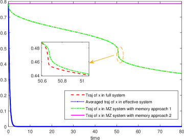
   (a) $\tau=2$, $\omega=10$

   

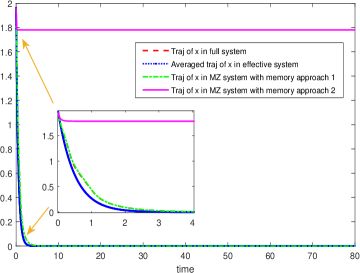
   (b) $\tau=0.2$, $\omega=4$

   Figure 4. Trajectories of $\mathbf{h}_{t}$ evolving under (4.2), (3.12), (3.10) (Approach 1) and (3.14) (Approach 2), respectively shown in red, green, blue and magenta. Parameters of $V$ are $\lambda=20$, $\mu=2$, and the time step was $\Delta t=10^{-5}$ and $T=80$.

   

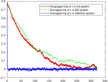
   (a) $\beta=1$

   

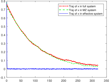
   (b) $\beta=10$

   

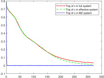
   (c) $\beta=100$

   Figure 5. Trajectories of $\mathbf{h}_{t}$ averaged over 500 trajectories of (2.1), (4.3) and (4.4), with identical realisations of Brownian motion in each case. Parameters of $V$ are $\lambda=20$ and $\mu=2$, $\tau=2$, $\omega=10$, and the time step was $\Delta t=10^{-5}$, total time was $T=320$.

2. Simulations with thermostat. We next included the thermostat once more, considering sample averages of the effective dynamics

   $$d\mathbf{h}_{t} =-\frac{\mu\mathbf{h}_{t}}{1+\tau^{2}\omega^{2}\cos^{2}(\omega\mathbf{h}_{t})}dt+\sqrt{\frac{2\beta^{-1}\Phi\Phi^{T}}{1+\tau^{2}\omega^{2}\cos^{2}(\omega\mathbf{h}_{t})}}d\mathbf{B}_{t}$$ (4.3)

   $$d\mathbf{h}_{t} =-\mu\mathbf{h}_{t}+\sqrt{2\beta^{-1}\Phi\Phi^{T}}d\mathbf{B}_{t}.$$ (4.4)

   For comparison, we again sampled the true dynamics of $\mathbf{h}_{t}$ including the thermostat, i.e.

   $$d\mathbf{F}(\mathbf{X}_{t})=-\Phi\nabla V(\mathbf{X}_{t})dt+\sqrt{2\beta^{-1}}\Phi d\mathbf{B}_{t}.$$ (2.3)

   Simulations were performed at different choices of inverse temperature, and averages were taken over 500 identical realisations of the Brownian motion, aiming to minimise statistical error. In each case, initial conditions were chosen such that

   $$\cos(\omega X_{0})=0,\qquad Y_{0}=\tau\sin(\omega Z_{0}).$$

   The results of this simulation are shown in Figure 5.

   Consistent with our observation that the effective dynamics (3.10) is independent of $\beta$, we observe good agreements between (4.3) and the full dynamics for all choices of $\beta$, with increasing accuracy as $\beta\to\infty$. In comparison, (4.4) reflects the dynamical properties of the system poorly in all cases.

5. conclusion

In this paper, we have employed the Mori–Zwanzig framework to rigorously derive an effective equation for linear reaction coordinates, describing features of an underlying overdamped Langevin dynamics. Such models are appropriate for a variety of applications where we wish to capture only limited aspects of a complex model, such as MD systems in the high friction limit. The equation we derived enables us to understand the sources of error and thereby inform a choice of effective dynamics which better captures dynamical features of the evolution which are not well–represented by the dynamics of the effective potential alone. We hope that this approach can serve to aid practitioners in understanding the sources of error in a coarse–grained model, particularly in the presence of entropic barriers.

We validated our analytic results by considering a benchmark example of overdamped Langevin system in a case where relaxation is impeded by a winding free energy barrier. This necessitated the careful asymptotic treatment of interactions between resolved and unresolved variables in order to correctly capture the dynamical behaviour of the system. In particular, although a time-scale separation occurs within the system we considered, we nevertheless showed that careful asymptotic analysis or dynamical sampling is required in general to ensure accuracy. The approximate model we constructed based upon the equations we derived exhibited a drastic improvement in predicting the dynamical behaviour of the reaction coordinates over the common approach of using the effective potential alone to describe the dynamics.

Our work prompts several questions, which we hope to address in future:

1. Practical sampling algorithms and error analysis. It would be of practical interest to devise an algorithm to generate effective dynamics based on the asymptotic approximation we considered here, and conduct a rigorous error analysis in this case.

2. Extensions to nonlinear coarse–grained variables and full Langevin dynamics. In this work, we have considered the overdamped Langevin setting with linear reaction coordinates. It would be of significant interest to extend this analysis to nonlinear variables and full Langevin dynamics using our reliable asymptotic analysis approach in future.

Appendix A Proof of Theorem 2.1

In this section, we provide a proof of our main mathematical result, Theorem 2.1. The proof follows a similar strategy to other derivations using the Mori–Zwanzig formalism given in the literature, notably [10, 21, 25].

A.1. Construction of ‘orthogonal’ variables

Our first step to construct variables which capture directions in phase space which are ‘orthogonal’ to those captured by the reaction coordinates $\mathbf{F}$, i.e. a foliation of the phase space.

Recall that $\Phi\in\mathbb{R}^{m\times N}$ is a matrix of full rank by assumption, and therefore it follows that the symmetric strictly positive definite square root matrix $\Sigma:=\sqrt{\Phi\Phi^{T}}\in\mathbb{R}^{m\times m}$ exists. Recalling the construction of the singular value decomposition, we find that there exist orthogonal matrices $U\in\mathbb{R}^{m\times m}$ and $V\in\mathbb{R}^{N\times N}$ such that

$$\Sigma^{-1}\Phi=UDV^{T},\quad\text{where}\quad D=\left(\begin{array}[]{cc}\mathrm{I}_{m}&0\end{array}\right)\in\mathbb{R}^{m\times N},$$

where $\mathrm{I}_{m}\in\mathbb{R}^{m\times m}$ is the identity matrix, and $0$ denotes a submatrix of zeros. Defining

$$E:=\left(\begin{array}[]{cc}0&\mathrm{I}_{N-m}\end{array}\right)\in\mathbb{R}^{(N-m)\times N},$$

where again $\mathrm{I}_{N-m}\in\mathbb{R}^{(N-m)\times(N-m)}$ is an identity matrix and $0$ denotes a matrix of zeros, we set

$$\Psi:=EV^{T}\in\mathbb{R}^{(N-m)\times N},\qquad\text{and}\qquad\Phi^{*}:=\Phi^{T}\Sigma^{-2}\in\mathbb{R}^{N\times m}$$

and it follows that

$$\Phi^{*}\Phi+\Psi^{T}\Psi=\mathrm{I}_{N\times N}.$$ (A.1)

From the construction above, we see that $\Phi^{*}\Phi\in\mathbb{R}^{N\times N}$ is an orthogonal projection acting on the phase space $\mathbb{R}^{N}$, and the matrix $\Psi$ ‘selects’ exactly the unresolved variables, so that if $\Phi\mathbf{x}=\mathbf{h}$ and $\Psi\mathbf{x}=\widetilde{\mathbf{x}}$, we have

$$\mathbf{x}=\Phi^{*}\Phi\mathbf{x}+\Psi^{T}\Psi\mathbf{x}=\Phi^{*}\mathbf{h}+\Psi^{T}\widetilde{\mathbf{x}}.$$

Given $\Phi$, we may use the construction of $\Psi$ in order to define the partition function $Z_{\Phi}:\mathbb{R}^{m}\to\mathbb{R}$,

$$Z_{\Phi}(\mathbf{h}):=\int e^{-\beta V(\Phi^{*}\mathbf{h}+\Psi^{T}\widetilde{\mathbf{x}})}d\widetilde{\mathbf{x}}.$$

A.2. Dyson–Duhamel principle

Next, we define

$$\mathbf{h}_{t}(\mathbf{x})=\mathbb{E}\big{[}\mathbf{F}(\mathbf{x}_{t})\,\big{|}\,\mathbf{x}_{0}=\mathbf{x}\big{]}.$$

Applying the Feynman–Kac formula, we recall that $\mathbf{h}_{t}$ solve the PDE

$$\partial_{t}\mathbf{h}_{t}=\mathcal{L}\mathbf{h}_{t}=-\nabla V\cdot\nabla\mathbf{h}_{t}+\beta^{-1}\Delta\mathbf{h}_{t},\quad\text{with}\quad\mathbf{h}_{0}(\mathbf{x})=\mathbf{F}(\mathbf{x}).$$

In semigroup notation, we will write $\mathbf{h}_{t}=e^{t\mathcal{L}}\mathbf{F}$, and so the Feynman–Kac formula becomes

$$\partial_{t}\mathbf{h}_{t}=e^{t\mathcal{L}}\mathcal{L}\mathbf{F}.$$ (A.2)

Given mutually orthogonal projection operators $\mathcal{P}$ and $\mathcal{Q}$, applying the Dyson–Duhamel principle entails that we have the identity

$$e^{t\mathcal{L}}=\int_{0}^{t}e^{(t-s)\mathcal{L}}\mathcal{P}\mathcal{L}e^{s\mathcal{Q}\mathcal{L}}ds+e^{t\mathcal{Q}\mathcal{L}},$$ (A.3)

which can be verified by differentiation with respect to $t$. Writing $\mathcal{L}\mathbf{F}=\mathcal{P}\mathcal{L}\mathbf{F}+\mathcal{Q}\mathcal{L}\mathbf{F}$ in (A.2) and applying (A.3), we find that

$$\partial_{t}\mathbf{h}_{t}=e^{t\mathcal{L}}\mathcal{P}\mathcal{L}\mathbf{F}+\int_{0}^{t}e^{(t-s)\mathcal{L}}\mathcal{P}\mathcal{L}e^{s\mathcal{Q}\mathcal{L}}\mathcal{Q}\mathcal{L}\mathbf{F}\,ds+e^{t\mathcal{Q}\mathcal{L}}\mathcal{Q}\mathcal{L}\mathbf{F}.$$ (A.4)

Our main focus will now be on the first two terms in (A.4), since the latter term is $\mathcal{F}_{t}$ as defined in (2.12). To rewrite the former term, we apply the definition of projection operator $\mathcal{P}$, the definitions of $\Phi$, $\Psi$ and $Z_{\Phi}$ and the chain rule, giving

$$\mathcal{P}\mathcal{L}\mathbf{F}(\mathbf{x})=\Sigma^{2}\,\mathbb{E}\big{[}-\Sigma^{-2}\Phi\nabla V\,\big{|}\,\mathbf{F}(\mathbf{x})\big{]}\\ =\frac{\Sigma^{2}}{Z_{\Phi}\big{(}\mathbf{F}(\mathbf{x})\big{)}}\int-(\Phi^{*})^{T}\nabla V(\Phi^{*}\,\mathbf{F}(\mathbf{x})+\Psi^{T}\widetilde{\mathbf{x}})e^{-\beta V(\Phi^{*}\,\mathbf{F}(\mathbf{x})+\Psi^{T}\widetilde{\mathbf{x}})}d\widetilde{\mathbf{x}}=-\Sigma^{2}\nabla\mathcal{S}\big{(}\mathbf{F}(\mathbf{x})\big{)},$$

where we recall the definition of the effective potential $\mathcal{S}$ given in (2.10).

A.3. Orthogonal dynamics

Next, we consider the action of $e^{s\mathcal{Q}\mathcal{L}}$, which will subsequently allow us to treat the integral term in (A.4). We begin by noting that

$$\mathcal{Q}\mathcal{L}\mathbf{F}(\mathbf{x})=\mathcal{L}\mathbf{F}(\mathbf{x})-\mathcal{P}\mathcal{L}\mathbf{F}(\mathbf{x})=-\Phi\nabla V(\mathbf{x})+\Sigma^{2}\nabla\mathcal{S}\big{(}\mathbf{F}(\mathbf{x})\big{)},$$

and define $\mathbf{g}_{t}:\mathbb{R}^{N}\to\mathbb{R}^{m}$ to be the solution to

$$\partial_{t}\mathbf{g}_{t}(\mathbf{x})=\mathcal{Q}\mathcal{L}\mathbf{F}(\mathbf{x})\cdot\nabla\mathbf{g}_{t}(\mathbf{x}),\qquad\mathbf{g}_{0}(\mathbf{x})=\mathcal{Q}\mathcal{L}\mathbf{F}(\mathbf{x});$$

using semigroup notation, we write this as $\mathbf{g}_{s}=e^{s\mathcal{Q}\mathcal{L}}\mathcal{Q}\mathcal{L}\mathbf{F}$.

Under assumptions (1) and (2) made in Section 2, it can be verified that $\Sigma^{2}\nabla\mathcal{S}\circ\mathbf{F}$ is globally Lipschitz. Using this fact, it can therefore be shown using the method of characteristics that $\mathbf{g}_{s}$ exists and is a $C^{1}$ diffeomorphism on $\mathbb{R}^{N}$; for similar results in the Hamiltonian setting, see [21].

Moreover, defining $\mathbf{a}_{s}:=\mathbf{g}_{s}(\mathbf{x})\in\mathbb{R}^{m}$ and $\mathbf{b}_{s}:=\mathbf{g}_{s}(\mathbf{y})\in\mathbb{R}^{m}$, then we use the fact that $\nabla\mathcal{S}$ and $\nabla V$ are Lipschitz along with Young’s inequality to deduce that

$$\frac{d}{ds}\frac{1}{2}\left|\mathbf{a}_{s}-\mathbf{b}_{s}\right|^{2}$$

$$\qquad=-\Big{(}\Phi\nabla V(\Phi^{*}\mathbf{a}_{s}+\Psi^{T}\Psi\mathbf{x})-\Phi\nabla V(\Phi^{*}\mathbf{b}_{s}+\Psi^{T}\Psi\mathbf{y})-\Sigma^{2}\nabla\mathcal{S}(\mathbf{a}_{s})+\Sigma^{2}\nabla\mathcal{S}(\mathbf{b}_{s})\Big{)}\cdot(\mathbf{a}_{s}-\mathbf{b}_{s}),$$

$$\qquad\lesssim\Big{(}\big{|}\Phi^{*}(\mathbf{a}_{s}-\mathbf{b}_{s})+\Psi^{T}\Psi(\mathbf{x}-\mathbf{y})\big{|}+|\mathbf{a}_{s}-\mathbf{b}_{s}|\Big{)}|\mathbf{a}_{s}-\mathbf{b}_{s}|,$$

$$\qquad\lesssim|\mathbf{a}_{s}-\mathbf{b}_{s}|^{2}+|\mathbf{x}-\mathbf{y}|^{2}.$$

Applying Gronwall’s inequality in the usual way, it follows that there exists $\alpha>0$ such that

$$|\mathbf{g}_{s}(\mathbf{x})-\mathbf{g}_{s}(\mathbf{y})|\leq|\mathbf{x}-\mathbf{y}|\sqrt{s}e^{\alpha s},\qquad\text{and thus}\qquad|\nabla\mathbf{g}_{s}(\mathbf{x})|\leq\sqrt{s}e^{\alpha s}.$$ (A.5)

A.4. Memory integral

Now that we have established properties of $\mathbf{g}_{s}$, we return to the integral term in (A.4). For now, we fix $\mathbf{x}\in\mathbb{R}^{N}$, and set $\mathbf{h}:=\mathbf{F}(\mathbf{x})$.

Consider $\mathcal{P}\mathcal{L}\mathbf{g}_{s}$; using the partition of the identity constructed in (A.1) we may write

$$\begin{split}&\mathcal{P}\mathcal{L}\mathbf{g}_{s}(\mathbf{x})\\ &\quad=\frac{1}{Z_{\Phi}(\mathbf{h})}\int\Big{(}-\nabla\mathbf{g}_{s}(\Phi^{*}\mathbf{h}+\Psi^{T}\widetilde{\mathbf{x}})\cdot\nabla V(\Phi^{*}\mathbf{h}+\Psi^{T}\widetilde{\mathbf{x}})+\beta^{-1}\Delta\mathbf{g}_{s}(\Phi^{*}\mathbf{h}+\Psi^{T}\widetilde{\mathbf{x}})\Big{)}e^{-\beta V(\Phi^{*}\mathbf{h}+\Psi^{T}\widetilde{\mathbf{x}})}d\widetilde{\mathbf{x}}\\ &\quad=\frac{1}{Z_{\Phi}(\mathbf{h})}\int\Big{(}-\nabla\mathbf{g}_{s}(\Phi^{*}\mathbf{h}+\Psi^{T}\widetilde{\mathbf{x}})\Phi^{*}\Phi\nabla V(\Phi^{*}\mathbf{h}+\Psi^{T}\widetilde{\mathbf{x}})+\beta^{-1}\Delta\mathbf{g}_{s}(\Phi^{*}\mathbf{h}+\Psi^{T}\widetilde{\mathbf{x}})\Phi^{*}\Phi\\ &\hskip 113.81102pt-\nabla\mathbf{g}_{s}(\Phi^{*}\mathbf{h}+\Psi^{T}\widetilde{\mathbf{x}})\Psi^{T}\Psi\nabla V(\Phi^{*}\mathbf{h}+\Psi^{T}\widetilde{\mathbf{x}})+\beta^{-1}\Delta\mathbf{g}_{s}(\Phi^{*}\mathbf{h}+\Psi^{T}\widetilde{\mathbf{x}})\Psi^{T}\Psi\Big{)}\\ &\hskip 369.88582pt\times e^{-\beta V(\Phi^{*}\mathbf{h}+\Psi^{T}\widetilde{\mathbf{x}})}d\widetilde{\mathbf{x}}.\end{split}$$

We collect terms involving matrix products with $\Phi$ and $\Psi$ separately, and using the chain rule, we find that

$$\begin{split}\mathcal{P}\mathcal{L}\mathbf{g}_{s}(\mathbf{x})&=\underbrace{\frac{1}{Z_{\Phi}(\mathbf{h})}\int\mathsf{div}_{\widetilde{\mathbf{x}}}\left(\frac{1}{\beta}\nabla_{\widetilde{\mathbf{x}}}\mathbf{g}_{s}(\Phi^{*}\mathbf{h}+\Psi^{T}\widetilde{\mathbf{x}})e^{-\beta V(\Phi^{*}\mathbf{h}+\Psi^{T}\widetilde{\mathbf{x}})}\right)d\widetilde{\mathbf{x}}}_{=:T_{1}}\\ &\hskip 34.1433pt+\underbrace{\frac{1}{Z_{\Phi}(\mathbf{h})}\int\mathsf{div}_{\mathbf{h}}\left(\frac{1}{\beta}\nabla_{\mathbf{h}}\mathbf{g}_{s}(\Phi^{*}\mathbf{h}+\Psi^{T}\widetilde{\mathbf{x}})\Sigma^{2}e^{-\beta V(\Phi^{*}\mathbf{h}+\Psi^{T}\widetilde{\mathbf{x}})}\right)d\widetilde{\mathbf{x}}}_{=:T_{2}},\end{split}$$

where subscripts denote the variable with respect which derivatives are taken. In particular, in the formula above, $\mathbf{g}_{s}(\Phi^{*}\mathbf{h}+\Psi^{T}\mathbf{x})$ is treated as a composition of functions. We now consider each of the terms $T_{1}$ and $T_{2}$ separately.

To treat $T_{1}$, we apply the divergence theorem. Truncating the domain of integration to $B_{R}(0)\subset\mathbb{R}^{N-m}$, a ball of radius $R$ centred at $0$, and considering the limit as $R\to\infty$, we have

$$\begin{split}T_{1}&=\frac{1}{Z_{\Phi}(\mathbf{h})}\lim\limits_{R\rightarrow\infty}\int_{B_{R}(0)}\mathsf{div}_{\widetilde{\mathbf{x}}}\left(\frac{1}{\beta}\nabla_{\widetilde{\mathbf{x}}}\mathbf{g}_{s}(\Phi^{*}\mathbf{h}+\Psi^{T}\widetilde{\mathbf{x}})e^{-\beta V(\Phi^{*}\mathbf{h}+\Psi^{T}\widetilde{\mathbf{x}})}\right)d\widetilde{\mathbf{x}}\\ &=\frac{1}{Z_{\Phi}(\mathbf{h})}\lim\limits_{R\rightarrow\infty}\int_{\partial B_{R}(0)}\left(\frac{1}{\beta}\nabla_{\widetilde{\mathbf{x}}}\mathbf{g}_{s}(\Phi^{*}\mathbf{h}+\Psi^{T}\widetilde{\mathbf{x}})e^{-\beta V(\Phi^{*}\mathbf{h}+\Psi^{T}\widetilde{\mathbf{x}})}\right)\cdot\vec{\nu}\,d\widetilde{S}.\end{split}$$ (A.6)

Applying (A.5) and the growth assumptions on $V$ to pass to the limit, we see that $T_{1}=0$.

For $T_{2}$, we note that we may commute differentiation and integration, and so multiplying and dividing by $Z_{\Phi}(\mathbf{h})$, we obtain, we obtain

$$\begin{split}T_{2}&=\frac{1}{Z_{\Phi}(\mathbf{h})}\mathsf{div}_{\mathbf{h}}\left(\int\frac{1}{\beta}\nabla_{\mathbf{h}}\mathbf{g}_{s}(\Phi^{*}\mathbf{h}+\Psi^{T}\widetilde{\mathbf{x}})\Sigma^{2}e^{-\beta V(\Phi^{*}\mathbf{h}+\Psi^{T}\widetilde{\mathbf{x}})}d\widetilde{\mathbf{x}}\right)\\ &=\frac{1}{Z_{\Phi}(\mathbf{h})}\mathsf{div}_{\mathbf{h}}\left(\frac{Z_{\Phi}(\mathbf{h})}{\beta}\frac{1}{Z_{\Phi}(\mathbf{h})}\int\nabla_{\mathbf{h}}\mathbf{g}_{s}(\Phi^{*}\mathbf{h}+\Psi^{T}\widetilde{\mathbf{x}})\Sigma^{2}e^{-\beta V(\Phi^{*}\mathbf{h}+\Psi^{T}\widetilde{\mathbf{x}})}d\widetilde{\mathbf{x}}\right).\end{split}$$ (A.7)

A.5. Memory kernel

To complete our analysis, we must show the identity

$$\mathcal{M}_{s}(\mathbf{h})=-\frac{1}{Z_{\Phi}(\mathbf{h})}\int\nabla_{\mathbf{h}}\mathbf{g}_{s}(\Phi^{*}\mathbf{h}+\Psi^{T}\widetilde{\mathbf{x}})\Sigma^{2}e^{-\beta V(\Phi^{*}\mathbf{h}+\Psi^{T}\widetilde{\mathbf{x}})}d\widetilde{\mathbf{x}},$$ (A.8)

where we recall that $\mathcal{M}_{s}$ was defined in (2.11).

Since we may again commute differentiation and integration, we use the product rule to write

$$\begin{split}&-\frac{1}{Z_{\Phi}(\mathbf{h})}\int\nabla_{\mathbf{h}}\mathbf{g}_{s}(\Phi^{*}\mathbf{h}+\Psi^{T}\widetilde{\mathbf{x}})\Sigma^{2}e^{-\beta V(\Phi^{*}\mathbf{h}+\Psi^{T}\widetilde{\mathbf{x}})}d\widetilde{\mathbf{x}}\\ &\quad=-\frac{1}{Z_{\Phi}(\mathbf{h})}\int\nabla_{\mathbf{h}}\left(\mathbf{g}_{s}(\Phi^{*}\mathbf{h}+\Psi^{T}\widetilde{\mathbf{x}})e^{-\beta V(\Phi^{*}\mathbf{h}+\Psi^{T}\widetilde{\mathbf{x}})}\right)\Sigma^{2}d\widetilde{\mathbf{x}}\\ &\quad\qquad-\frac{1}{Z_{\Phi}(\mathbf{h})}\int\mathbf{g}_{s}(\Phi^{*}\mathbf{h}+\Psi^{T}\widetilde{\mathbf{x}})\otimes\beta\,(\Phi^{*})^{T}\nabla V(\Phi^{*}\mathbf{h}+\Psi^{T}\widetilde{\mathbf{x}})e^{-\beta V(\Phi^{*}\mathbf{h}+\Psi^{T}\widetilde{\mathbf{x}})}\,\Sigma^{2}d\widetilde{\mathbf{x}}\\ &\quad=-\frac{1}{Z_{\Phi}(\mathbf{h})}\nabla_{\mathbf{h}}\left(\int\mathbf{g}_{s}(\Phi^{*}\mathbf{h}+\Psi^{T}\widetilde{\mathbf{x}})e^{-\beta V(\Phi^{*}\mathbf{h}+\Psi^{T}\widetilde{\mathbf{x}})}d\widetilde{\mathbf{x}}\right)\\ &\quad\qquad-\frac{1}{Z_{\Phi}(\mathbf{h})}\int\left(\mathbf{g}_{s}(\Phi^{*}\mathbf{h}+\Psi^{T}\widetilde{\mathbf{x}})\otimes\beta\,\Phi\nabla V(\Phi^{*}\mathbf{h}+\Psi^{T}\widetilde{\mathbf{x}})e^{-\beta V(\Phi^{*}\mathbf{h}+\Psi^{T}\widetilde{\mathbf{x}})}\right)d\widetilde{\mathbf{x}},\\ &\quad=\underbrace{-\frac{1}{Z_{\Phi}(\mathbf{h})}\nabla_{\mathbf{h}}\Big{(}Z_{\Phi}(\mathbf{h})\mathbb{E}[\mathbf{g}_{s}|\mathbf{F}(\mathbf{x})=\mathbf{h}]\Big{)}}_{=:T_{11}}+\underbrace{\vphantom{\frac{1}{Z_{\Phi}(\mathbf{h})}}\beta\,\mathbb{E}[\mathbf{g}_{s}\otimes\mathcal{L}\mathbf{F}|\mathbf{F}(\mathbf{x})=\mathbf{h}]}_{=:T_{12}}.\end{split}$$

Next, we recall that $\mathbf{g}_{s}=e^{s\mathcal{Q}\mathcal{L}}\mathbf{F}$, and $\mathcal{P}\mathcal{Q}=0$, so

$$\mathbb{E}\big{[}\mathbf{g}_{s}\big{|}\mathbf{F}(\mathbf{x})\big{]}=\mathbb{E}\big{[}e^{s\mathcal{Q}\mathcal{L}}\mathcal{Q}\mathcal{L}\mathbf{F}\big{|}\mathbf{F}(\mathbf{x})\big{]}=\left(\mathcal{P}\mathcal{Q}\mathcal{L}e^{s\mathcal{Q}\mathcal{L}}\mathbf{F}\right)(\mathbf{x})=0,$$ (A.9)

and therefore $T_{11}=0$. To treat $T_{12}$, we note that since $\mathcal{P}+\mathcal{Q}=\mathcal{I}$, we may split $T_{12}$ into

$$\begin{split}T_{12}&=\beta\,\mathbb{E}[e^{s\mathcal{Q}\mathcal{L}}\mathcal{Q}\mathcal{L}\mathbf{F}\otimes\mathcal{Q}\mathcal{L}\mathbf{F}|\mathbf{F}(\mathbf{x})=\mathbf{h}]+\beta\,\mathbb{E}[e^{s\mathcal{Q}\mathcal{L}}\mathcal{Q}\mathcal{L}\mathbf{F}\otimes\mathcal{P}\mathcal{L}\mathbf{F}|\mathbf{F}(\mathbf{x})=\mathbf{h}]\\ &=\mathcal{M}_{s}(\mathbf{h})+\beta\,\mathcal{P}e^{s\mathcal{Q}\mathcal{L}}\mathcal{Q}\mathcal{L}\mathbf{F}\otimes\mathcal{P}\mathcal{L}\mathbf{F}.\end{split}$$

Once again, the latter term vanishes thanks to (A.9), and so we have proved identity (A.8).

A.6. Conclusion of the proof

Applying identity (A.8) to (A.7) and using the product rule and the definition of the effective potential given in (2.10), we find that

$$T_{2}=\frac{1}{Z_{\Phi}(\mathbf{h})}\mathsf{div}\left(-\frac{Z_{\Phi}(\mathbf{h})}{\beta}\mathcal{M}_{s}(\mathbf{h})\right)=\mathcal{M}_{s}(\mathbf{h})\nabla\mathcal{S}(\mathbf{h})-\frac{1}{\beta}\mathsf{div}\mathcal{M}_{s}(\mathbf{h}).$$

Combining our analysis of each of the terms, we have therefore shown that

$$\partial_{t}\mathbf{h}_{t}=-\Sigma^{2}\nabla\mathcal{S}(\mathbf{h}_{t})+\int_{0}^{t}\mathcal{M}_{s}(\mathbf{h}_{t-s})\nabla\mathcal{S}(\mathbf{h}_{t-s})-\frac{1}{\beta}\mathsf{div}\mathcal{M}_{s}(\mathbf{h}_{t-s})\,ds+\mathcal{F}_{t}$$

Hence, we prove the theorem.

References

- [1] R. V. Abramov and A. J. Majda. Quantifying uncertainty for non-gaussian ensembles in complex systems. SIAM Journal on Scientific Computing, 26:411–447, 2004.
- [2] M. Berkowitz, J. Morgan, and J. A. McCammon. Generalized Langevin dynamics simulations with arbitrary time-dependent memory kernels. The Journal of Chemical Physics, 78:3256, 1983.
- [3] B. J. Berne and R. Pecora. Dynamic light scattering: With applications to chemistry, biology, and physics. Dover: New York, 2000.
- [4] M. Branicki and A. J. Majda. Quantifying uncertainty for predictions with model error in non-Gaussian systems with intermittency. Nonlinearity, 25(9), 2012.
- [5] M. Branicki and A. J. Majda. An information-theoretic framework for improving imperfect dynamical predictions via multi-model ensemble forecasts. Journal of Nonlinear Science, 25:489–538, 2015.
- [6] M. Chen, X. Li, and C. Liu. Computation of the memory functions in the generalized Langevin models for collective dynamics of macromolecules. The Journal of Chemical Physics, 141:064112, 2014.
- [7] A. Chorin and P. Stinis. Problem reduction, renormalization, and memory. Communications in Applied Mathematics and Computational Science, 1:1–27, 2006.
- [8] A. J. Chorin and O. H. Hald. In Stochastic Tools in Mathematics and Science. Springer, 2013.
- [9] A. J. Chorin, O. H. Hald, and R. Kupferman. Optimal prediction and the mori–zwanzig representation of irreversible processes. Proceedings of the National Academy of Sciences of the United States of America, 97:6253–6257, 2000.
- [10] A. J. Chorin, O. H. Hald, and R. Kupferman. Optimal prediction with memory. Physica D, 166:239–257, 2002.
- [11] A. J. Chorin and F. Lu. Discrete approach to stochastic parametrization and dimension reduction in nonlinear dynamics, 2015.
- [12] E. Darve, J. Solomon, and A. Kia. Computing generalized Langevin equations and generalized Fokker–Planck equations. Proceedings of the National Academy of Sciences of the United States of America, 106:10884–10889, 2009.
- [13] N. di Pasquale, D. Marchisio, and P. Carbone. Mixing atoms and coarse-grained beads in modelling polymer melts. The Journal of Chemical Physics, 137(16):164111, 2012.
- [14] M. Dobson. Information theoretic fitting for coarse-grained molecular dynamics. preprint. 2016 SIAM Conference on Mathematical Aspects of Materials Science.
- [15] W. E. In Principles of Multiscale Modeling. Cambridge University Press, 2011.
- [16] W. E, B. Engquist, X. Li, W. Ren, and E. Vanden-Eijnden. Heterogeneous multiscale methods: A review. Communications in Computational Physics, 2:367–450, 2007.
- [17] P. Espanol and P. Warren. Statistical mechanics of dissipative particle dynamics. Europhysics Letters, 30:191, 1995.
- [18] D. J. Evans and G. Morriss. Statistical mechanics of nonequilibrium liquids. Cambridge University Press, 2008.
- [19] G. W. Ford, M. Kac, and P. Mazur. Statistical mechanics of assemblies of coupled oscillators. Journal of Mathematical Physics, 6:504–515, 1965.
- [20] M. Frank and B. Seibold. Optimal prediction for radiative transfer: A new perspective on moment closure. Kinetic and Related Models, 4:717–733, 2011.
- [21] D. Givon, R. Kupferman, and O. H. Hald. Existence proof for orthogonal dynamics and the Mori-Zwanzig formalism. Israel Journal of Mathematics, 145(1):221–241, Dec 2005.
- [22] I. Grooms and A. J. Majda. Efficient stochastic superparameterization for geophysical turbulence. Proceedings of the National Academy of Sciences of the United States of America, 110:4464–4469, 2013.
- [23] N. Guttenberg, J. F. Dama, M. G. Saunders, G. A. Voth, J. Weare, and A. R. Dinner. Minimizing memory as an objective for coarse-graining. The Journal of Chemical Physics, 138:094111, 2013.
- [24] C. Hartmann. Model reduction in classical molecular dynamics, 2007. PhD Thesis. Fachbereich Mathematik und Informatik Freie Universitat Berlin.
- [25] C. Hijón, P. Español, E. Vanden-Eijndenc, and R. Delgado-Buscalioni. Mori–Zwanzig formalism as a practical computational tool. Faraday Discussions, 144:301–322, 2010.
- [26] S. Izvekov and G. A. Voth. Modeling real dynamics in the coarse-grained representation of condensed phase systems. Journal of Chemical Physics, 125:151101–151104, 2006.
- [27] M. A. Katsoulakis and P. Plechac. Information-theoretic tools for parametrized coarse-graining of non-equilibrium extended systems. The Journal of Chemical Physics, 139:74–115, 2013.
- [28] T. Kinjo and S. aki Hyodo. Equation of motion for coarse-grained simulation based on microscopic description. Physical Review E, 75:051109, 2007.
- [29] S. Klus, F. Nüske, P. Koltai, H. Wu, I. Kevrekidis, C. Schütte, and F. Noé. Data-driven model reduction and transfer operator approximation. Journal of Nonlinear Science, 28:985–1010, 2018.
- [30] F. Legoll and T. Lelievre. Effective dynamics using conditional expectations. Nonlinearity, 23:2131–2163, 2010.
- [31] F. Legoll and T. Lelievre. Some remarks on free energy and coarse-graining. In Numerical Analysis and Multiscale Computations, B. Engquist, O. Runborg, R. Tsai eds., Springer Lecture Notes in Computational Science and Engineering, volume 82, pages 279–329. Springer, 2012.
- [32] F. Legoll, T. Lelievre, and S. Olla. Pathwise estimates for an effective dynamics. Stochastic Processses and their Applications, 127:2841–2863, 2017.
- [33] F. Legoll, T. Lelievre, and U. Sharma. Effective dynamics for non-reversible stochastic differential equations: a quantitative study. manuscript.
- [34] H. Lei, N. Baker, and X. Li. Data-driven parameterization of the generalized Langevin equation. Proceedings of the National Academy of Sciences of the United States of America, 113:14183–14188, 2016.
- [35] H. Lei, B. Caswell, and G. E. Karniadakis. Direct construction of mesoscopic models from microscopic simulations. Physical Review E, 81:026704, 2010.
- [36] T. Lelièvre, M. Rousset, and G. Stoltz. In Free energy computations: A mathematical perspective. Imperial College Pressr, 2010.
- [37] T. Lelièvre and W. Zhang. Pathwise estimates for effective dynamics: the case of nonlinear vectorial reaction coordinates. 2018. hal-01794919.
- [38] X. Li. A coarse-grained molecular dynamics model for crystalline solids. International Journal for Numerical Methods in Engineering, 83:986–997, 2010.
- [39] Z. Li, X. Bian, X. Li, and G. E. Karniadakis. Incorporation of memory effects in coarse-grained modeling via the Mori-Zwanzig formalism. The Journal of Chemical Physics, 143:243128, 2015.
- [40] Z. Li, H. S. Lee, E. Darve, and G. E. Karniadakis. Computing the non-Markovian coarse-grained interactions derived from the Mori–Zwanzig formalism in molecular systems: application to polymer melts. The Journal of Chemical Physics, 146, 2017.
- [41] G. Lindgren. Stationary stochastic processes: Theory and applications. Chapman and Hall/CRC, 2012.
- [42] F. Lu, X. Tu, and A. J. Chorin. Accounting for model error from unresolved scales in ensemble kalman filters by stochastic parameterization, 2017.
- [43] L. Ma, X. Li, and C. Liu. Coarse-graining Langevin dynamics using reduced-order techniques, 2018. arxiv:1802.10133.
- [44] A. Majda and X. Wang. Nonlinear dynamics and statistical theories for basic geophysical flows. Cambridge University Press, 2006.
- [45] A. J. Majda. Introduction to turbulent dynamical systems in complex systems. In Frontiers in Applied Dynamical Systems: Reviews and Tutorials. Springer, 2016.
- [46] A. J. Majda, R. V. Abramov, and M. J. Grote. Information theory and stochastics for multiscale nonlinear systems. American Mathematical Society, 2005.
- [47] A. J. Majda, M. Branicki, and Y. Frenkel. Improving complex models through stochastic parameterization and information theory, 2011. ECMWF-WCRP, Thorpex Workshop on Model Uncertainty.
- [48] G. F. Mazenko. In Nonequilibrium Statistical Mechanics. Wiley-Vch, 2006.
- [49] H. Mori. Transport, collective motion, and Brownian motion. Progress of Theoretical Physics, 33(3):423–455, 1965.
- [50] T. Munakata. Generalized Langevin-equation approach to impurity diffusion in solids: perturbation theory. Physical Review B, 33:8017, 1985.
- [51] S. Nordholm and R. Zwanzig. A systematic derivation of exact generalized Brownian motion theory. Journal of Statistical Physics, 13(4):340–370, 1975.
- [52] N. D. Pasquale, T. Hudson, and M. Icardi. Systematic derivation of hybrid coarse-grained models, 2018. arxiv:1804.08157.
- [53] F. Pinski, G. Simpson, A. M. Stuart, and H. Weber. Algorithms for Kullback-Leibler approximation of probability measures in infinite dimensions. SIAM Journal on Scientific Computing, 37(6):2733–2757, 2014.
- [54] G. O. Roberts and R. L. Tweedie. Exponential convergence of Langevin distributions and their discrete approximations. Bernoulli, 2(4):341–363, 12 1996.
- [55] I. Snook. The langevin and generalised Langevin approach to the dynamics of atomic, polymeric and colloidal systems. Elsevier, Amsterdam, 2017.
- [56] P. Stinis. Renormalized Mori–Zwanzig-reduced models for systems without scale separation. Proceedings of the Royal Society A, 471:20140446, 2015.
- [57] T. D. Swinburne. Stochastic dynamics of crystal defects, 2015. PhD Thesis. Imperial College London, Department of Physics.
- [58] M. E. Velinova. In Coarse-grained Molecular Dynamics. Delve Pub, 2017.
- [59] D. Venturi, H. Cho, and G. E. Karniadakis. Mori-Zwanzig approach to uncertainty quantification. In Handbook of Uncertainty Quantification, pages 1–36. Springer, 2016.
- [60] Y. Yoshimoto, I. Kinefuchi, T. Mima, A. Fukushima, T. Tokumasu, and S. Takagi. Bottom-up construction of interaction models of non-Markovian dissipative particle dynamics. Physical Review E, 88:043305, 2013.
- [61] Y. Zhu, J. Dominy, and D. Venturi. On the estimation of the Mori-Zwanzig memory integral. Journal of Mathematical Physics, 59:103501, 2018.
- [62] Y. Zhu and D. Venturi. Faber approximation to the Mori-Zwanzig equation. Journal of Computational Physics, 372:694–718, 2018.
- [63] R. Zwanzig. Memory effects in irreversible thermodynamics. Physical Review, 124(4):983–922, 1961.
- [64] R. Zwanzig. Nonlinear generalized Langevin equations. Journal of Statistical Physics, 9:215–220, 1973.
- [65] R. Zwanzig. Nonequilibrium statistical mechanics. In Nonequilibrium statistical mechanics. Oxford University Press, 2001.