Combinatorialization of spaces of nondegenerate spherical curves
Victor Goulart
goulart@mat.puc-rio.brNicolau C. Saldanha
saldanha@puc-rio.brMathematics Department
PUC-Rio, Brazil
Abstract
A parametric curve of
class on the -sphere is said to be
nondegenerate (or locally convex) when
for all values of the parameter .
We orthogonalize this ordered basis to obtain
the Frenet frame of
assuming values in the orthogonal
group
(or its universal double cover, ),
which we decompose into Schubert or Bruhat cells.
To each nondegenerate curve we assign
its itinerary: a word in the
alphabet that
encodes the succession of non open Schubert cells
pierced by the complete flag of
spanned by the columns of .
Without loss of generality, we can focus on
nondegenerate curves with initial and final flags
both fixed at the (non oriented) standard complete flag.
For such curves, given a word , the subspace of curves
following the itinerary is a contractible
globally collared topological submanifold of finite codimension.
By a construction reminiscent of Poincaré duality,
we define abstract cell complexes mapped
into the original space of curves by
weak homotopy equivalences.
The gluing instructions come from a partial order in the
set of words.
The main aim of this construction is to attempt to determine
the homotopy type of spaces of nondegenerate curves for .
The reader may want to contrast
the present paper’s combinatorial approach
with the geometry-flavoured methods of
previous works.
1 Introduction
For a fixed positive integer ,
consider the -sphere
with respect to the usual Euclidean metric
of . A parametric curve
of class is said to be nondegenerate
[32, 33, 34, 40, 59, 65] or locally convex
[2, 51, 52, 53, 54]
if and only if its derivatives up to
order
span a complete flag
of for all .
Without loss of generality, we shall consider
only positive nondegenerate curves,
i.e., those satisfying
.
Consider the Frenet frame of a
nondegenerate curve
at time to be the orthogonal matrix
obtained
by Gram-Schmidt orthonormalization of the ordered basis
.
We denote by the same symbol the
Frenet curve just defined and its lift to the universal double cover
of the special orthogonal group, the group .
We denote by the resulting
space of nondegenerate curves satisfying
with the subspace topology
induced by the standard -norm of
. It is easily seen that
is contractible; fixing the final frame
at a definite element
produces subspaces .
Our main problem is to determine
the homotopy type of such subspaces. The present paper
provides a recipe for the construction of an abstract cell
complex weak homotopy equivalent to .
Consider the subgroup
of diagonal matrices and its lift .
The group is often called the Clifford group
(see [38]) and
is the classical quaternion group.
Define our working space of
nondegenerate curves as
(1)
the space of nondegenerate curves whose flags
begin and end at the standard complete flag
of .
It is shown in [54] that for each
we can determine explicitly an
element such that
the spaces and
are homeomorphic. Therefore, in order to understand
all the spaces , one may restrict attention
to the disjoint union of spaces
in Equation 1.
It is worth pointing out that some but not all
of the remaining spaces exhibit the same
homotopy type (see historical remarks below
and final remarks on Section 18).
For a number of technical reasons, we shift to a
slightly relaxed notion of nondegeneracy that replaces
each space with a homotopy equivalent
smooth Hilbert manifold
(see Appendix B).
We deliberately blur the distinction
between the original space and its Hilbert manifold
version by using the same notation for both throughout.
Since we are mainly interested
in describing homotopy types, this slight
abuse is mostly harmless.
Let be the group of permutations of
.
For , let
be the number of inversions of .
We denote by the set of finite words in the
alphabet .
For , set
,
where .
For , we define below its
itinerary .
Let be the set of curves with itinerary :
this yields a stratification
(2)
into topological submanifolds .
Theorem 1.
For each , there is a unique
such that
is a contractible globally collared submanifold of
of codimension .
In order to define the itinerary ,
recall the Bruhat decomposition
of the real general linear group
into double cosets
of the subgroup of invertible
real upper triangular matrices, indexed by the
group . The permutation matrix is defined by
.
We denote the image of the integer
under the permutation
by .
The above partition yields a cell decomposition
of the real complete flag variety
into Schubert cells , whose dimension is .
The (strong) Bruhat order on
[8, 30, 67]
is defined by if and only if
(with respect to either Zariski or the usual topology).
The Lie group is the
universal cover of the flag variety .
The unsigned Bruhat cells
are the -fold covers of the respective Schubert cells
;
we have if and only if .
Although these are well known facts
[7, 16, 17, 37, 67],
the aspects of the subject that are going to
bear on the proofs of Theorems 1 and
2 shall be derived from scratch
in the following sections, in a language specially adapted
to our purposes.
We shall often regard as a Coxeter-Weyl
group of type with transpositions
as generators. The Coxeter element
is the unique element with . The Bruhat cell
is an open dense subset of .
We show in Lemma 8.2 that
for each there are only
finitely many instants
at which
.
Let be such that .
Set .
By a construction similar to Poincaré duality,
we obtain from the stratification in Equation
2
a CW complex and a weak homotopy equivalence
.
Theorem 2.
There exists a CW complex with one cell
for each word
and a compatible family of continuous maps
. Compatibility means
that there exists a continuous map
defined by (for each ).
The map is a weak homotopy equivalence.
The sense in which this complex is a dual to the stratification
is explained in Section 15, particularly in the concept
of valid complexes.
The maps are constructed rather explicitly in Sections
11 and 15.
The map turns out to intersect only at ,
in a topologically transversal manner.
One important concept in this construction is a partial order
in the set of words .
We define if and only if
.
It turns out that the image
under is contained in strata for .
This combinatorial approach has already
allowed further progress on the subject, which we
expect to cover in a forthcoming paper
[3]. A sample may
be found in the conjectures stated in our final remarks
(Section 18).
The space
of closed nondegenerate curves
was originally studied by J. Little in the
seventies [40], and shown to have three
connected components: , containing
curves with an odd number of transversal
self-intersections; , the subspace of simple curves; and
, containing curves with positive even number
of self-intersections (we will make sense of this
notation in due course). The works of B. Khesin,
B. Shapiro and M. Shapiro in the nineties
[34, 59, 65]
extended this result for and
arbitrary, showing that has one or
two connected components: one if and only if it does not
contain convex curves (defined in Appendix
A) and two otherwise, one of
them being the contractible subspace of the said
convex curves. The former results are reobtained
in the present paper within our combinatorial framework.
In [54] it is shown that each space
is homeomorphic to one of the spaces
, ;
also, several among the latter are homeomorphic.
In [53] the spaces were
completely classified into three homotopy types explicitly described.
The analogous problem of describing the homotopy
types of the spaces for is currently open.
We hope to contribute to this problem, in particular
solving it for , in a subsequent paper
[3] using the
combinatorial framework proposed in the present
work (see conjectures in our final remarks, Section
18). Some partial results for
were obtained in [2] by
different methods, more akin to those of [53].
One common motivation for the study of such problems
is the study of linear ordinary differential operators
[47].
This point of view was the original motivation of B. Khesin
and B. Shapiro for considering the problem in the
early nineties
[32, 33, 34, 61].
The second named author was first led to consider
this problem while studying the topology and geometry of critical
sets of nonlinear differential operators with periodic
coefficients, in a series of works with D. Burghelea
and C. Tomei
[13, 14, 15, 55]
In Section 2 we review some basics of the symmetric group: useful representations of a permutation and the poset structures given by the strong and weak Bruhat orders. We also introduce the multiplicities of a permutation.
In Section 3,
we study the hyperoctahedral group and the double cover
of .
We are particularly interested in the maps and , which will
come up constantly in our discussion.
In Section 4 we introduce
triangular systems of coordinates in large open subsets
of the group and study
locally convex curves in the nilpotent lower triangular group
.
In Section 5 we recall the important concept
of total positivity. More generally, we define the subsets
for .
We review some classical results and prove some useful facts.
In Section 6, we consider the related concept of
accessibility in the triangular group and prove the contractibility
of certain sets which will come up later.
In Section 7 we prove several useful results
about the well known stratification of the group
in Bruhat cells. We also recall the useful notion of projective transformations.
In Section 8 we review the chopping operation defined in [54] and introduce the dual notion of advancing.
We also study the singular set of a locally convex curve :
the set of values of for
which .
In Section 9, we revisit the concept of accessibility,
now in the spin group. We prove the contractibility of several
subsets of .
Section 10 contains the proof of
Theorem 1, divided in a series of lemmas.
In Section 11 we construct the restriction
to an open ball around the origin of the cell
in the complex .
In Section 12 we define the
multiplicity vector for a word and study a few examples
of the restrictions constructed in Section 11.
In Section 13 we prove a few basic necessary facts
about the partial order defined in .
Section 14 contains a few remarks about
lower and upper subsets of the poset .
In Section 15 we prove Theorem 2.
In Sections 16 and 17 we explicitly construct
the and -skeletons of the complex .
As a corollary, we obtain the well known classification of
connected components of .
The -skeleton is of course a key ingredient towards proving
the simple connectivity of connected components of
(see Conjecture 18.3).
Section 18 contain our final remarks,
with an emphasis on results which we expect to prove in a
forthcoming paper [3]
and which are stated here as conjectures.
Appendix A reviews the notion of convexity
of spherical curves and studies its relation with the notion of itinerary.
In Appendix B we define precisely the
smooth Hilbert manifold homeomorphic to to which
Theorems 1 and 2 apply.
This paper is an extended version of the Ph.D. thesis
[26] of the first author, supervised by the second.
The first named author is grateful to his co-advisor
Boris Khesin for the warm hospitality during his time
as a visiting graduate student at the
Department of Mathematics of the University of Toronto.
The second author thanks the kind hospitality of Stockholm
University during his visits.
Both authors would like to thank Emília Alves, Boris Khesin,
Ricardo Leite, Carlos Gustavo Moreira,
Paul Schweitzer, Boris Shapiro, Carlos Tomei,
David Torres, Cong Zhou and Pedro Zülkhe for helpful conversations
and gratefully acknowledge the financial support of
PUC-Rio, CAPES, CNPq and FAPERJ (Brazil).
2 The symmetric group
Consider the symmetric group
(acting on )
as the Coxeter-Weyl group , i.e.,
use the generators
, , …, .
For and
we use the notation (rather than )
so that .
A permutation can be denoted in many ways:
one common notation is as a list of values
,
the so called complete notation;
another is as a product of the generators above;
for instance, . Notice that
we enclose between brackets a expression
of a permutation in terms of Coxeter generators.
We adopt this device to avoid confusion
between the single permutation with that expression and
a string of generators with no product intended. Strings of
permutations are to appear prominently in this paper,
encoding the so called itinerary of a nondegenerate
curve.
For , let be
the permutation matrix defined by
;
for instance, for we have:
For , let be the length of
with the generators ,
(we reserve the symbol for lengths of the itineraries mentioned above).
Equivalently,
is the number of inversions of ;
the set of inversions is
A set
is the set of inversions of a permutation
if and only if
Also, if then
.
Let
be the nilpotent triangular groups
of real upper and lower triangular matrices
with all diagonal entries equal to .
For consider the subgroups
(3)
affine subspaces of dimension .
If then
any can be written uniquely as
, , .
A reduced word for is an identity
or, more formally, it is a finite sequence of indices
satisfying the identity above.
Two reduced words for the same permutation
are connected by a finite sequence of local moves of two kinds:
(4)
(5)
corresponding to the identities for
and , respectively.
Recall that there exists a unique
with , the Coxeter element
(elsewhere usually denoted by : we spare the letter
for itineraries, as mentioned above);
write
Recall that the (strong) Bruhat order in the symmetric group
can be defined as follows: if
some reduced word for is a substring of some reduced word for
(a substring here need not have consecutive letters).
Write if
is an immediate predecessor of
(in the Bruhat order).
Recall that
if and
;
here , ,
, ,
, .
We have
(with )
if and only if there exist with
If is written as ,
it is easy to find its immediate predecessors:
look for integers appearing in the list
,
to the left of ,
such that the integers which appear in the list between and
are either larger than or smaller than ;
the permutation is then obtained
by switching the entries and .
In the matrix , we must look for positive entries
, such that the interior of the rectangle
with these vertices includes no positive entry. Then
is obtained by flipping these entries
to the diagonal position while leaving the complement
of the rectangle unchanged.
The strong Bruhat order must not be confused with the left ang right
weak Bruhat orders.
Define the weak left Bruhat order
by taking the transitive closure of:
if
and (for some ).
Equivalently, if
.
Similarly,
if
and (for some );
the transitive closure
is characterized by .
Notice that either
or
imply ;
on the other hand,
,
but and .
For more on Coxeter groups and Bruhat orders, see [8, 30].
Lemma 2.1.
Consider and
such that .
Then
if and only if
.
Similarly, if and only if
.
Proof.
The condition
is equivalent to .
But
and ,
proving the first equivalence.
The second one is similar.
∎
Define
A simple computation verifies that
We may therefore recursively define
the previous remarks, together with the connectivity of reduced words
under the moves in Equations 4 and 5,
show that this is well defined.
Equivalently, is the smallest
(in the strong Bruhat order) satisfying both
and .
Notice that is not a lattice with the strong Bruhat order;
the operation above uses more than one partial order.
In general, we may have
and .
We do have associativity:
.
Example 2.2.
Take , ,
.
We have .
Another useful representation of a permutation is in terms of its
multiplicities, which we now define.
For and , let
With the convention ,
we have ,
so that the multiplicity vector easily
determines . The reason for calling
a multiplicity will become clear in section 12.
If we write
if, for all , .
If (in the Bruhat order)
then
and .
Example 2.3.
For , let and .
We have
but .
For , let and .
We have
and .
Lemma 2.4.
Let
with .
Then
Here we use Iverson notation:
Proof.
This is an easy computation.
∎
The notion of multiplicity is closely related
to a beautiful 1-1 correspondence, discovered
by S. Elnitsky [19], between commutation
classes of reduced words for a permutation
and the rhombic tilings of
a certain (possibly degenerate) -gon
associated to .
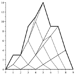
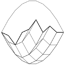
An equivalent (if somewhat deformed) version
of this construction is obtained by considering
tesselations by parallelograms of the plane region
between the graphs
of
and . These decompositions
can be performed directly on the graph of
, as shown in figure
1 below.
Figure 1: Conjugate tilings of the graph of
and of the
Elnitsky’s polygon for
corresponding
to the commutation class of the reduced word
.
3 Signed permutations
Let be the hyperoctahedral group of signed permutation matrices,
i.e., orthogonal matrices such that there exists a permutation
with for all .
The group is a Coxeter group (whence the notation)
but we shall not use this presentation.
Let .
Let
be the normal subgroup of diagonal matrices,
isomorphic to .
We have ,
the quotient map being denoted by .
Consider the universal double covering
of the special orthogonal group and let
and
.
The group has elements
and is a normal subgroup of ;
the quotient is again the symmetric group ;
In other words, we have the exact sequences
Recall that . The Clifford group
(see [38])
is a natural generalization of the classical quaternion group .
Let be the matrix with only two nonzero entries:
(6)
Consider given by and let and , so that .
The matrix has nonzero entries
is a rotation of in the plane
spanned by and .
Notice that .
Lemma 3.1.
The following identities hold:
Proof.
These are simple computations.
∎
Each element can be written
uniquely as
In particular, the elements , ,
generate .
Furthermore, if and
,
take :
we have and therefore
with .
In particular, the elements , ,
generate .
We make this construction more systematic.
Lemma 3.2.
If is expressed by two reduced words
then
.
Proof.
Both moves (as in Equations 4 and 5)
are taken care of by Lemma 3.1.
∎
Let .
For , take a reduced word
: set
Lemma 3.2 shows that the maps
are well defined.
Notice that these maps are not homomorphisms.
Similarly, non-reduced words do not work
in the above formulas for and ;
has order but has order .
Also, define
so that for all .
Notice that these notations are consistent
with the previously introduced special cases and .
Let where
notice that
and therefore .
Lemma 3.3.
For any and for any
we have
Proof.
The permutation restricts to a bijection between the two sets:
with cardinalities
and .
∎
Lemma 3.4.
Consider and set . We have
and therefore
The nonzero entries of are
We also have .
Proof.
The first expression for the diagonal entries of
follows directly from the first two formulae,
which we now prove by induction on .
The base cases are easy.
Assume ,
so that ,
where . By the induction hypotheses we have
To see that for all values of , consider separately the cases , , and . The second formula is similar. The alternate expressions for are obtained via Lemma 3.3.
Finally, setting
and we have
and therefore , hence .
∎
If then, by definition,
We show how to obtain a different recursive formula for .
these imply the formulas for .
We then have, for even,
and, for odd,
Finally, notice that even implies
and therefore
;
conversely, odd implies
and therefore .
∎
Lemma 3.6.
Let ,
.
1.
If is odd then
and .
2.
If is even then
and .
Proof.
We know (by definition) that
.
As in Lemma 3.5, write
.
We know from Lemma 3.4
that we can take .
Thus
If is odd then
and therefore and
.
If is even then
and therefore and
.
∎
Example 3.7.
Using this result it is easy to compute given .
Take, say, .
Take
We therefore have
Example 3.8.
We have that
is a reduced word so that
and .
From Lemma 3.4, we have and
Notice that, for odd, we have is in the center of .
Lemma 3.9.
Proof.
For we have if and only if , with and .
For we have if and only if with ,
.
Also, if and
only if , with
,
.
For , take
;
we have ,
.
∎
4 Triangular coordinates
Let be the nilpotent group of real lower triangular matrices
with all diagonal entries equal to ;
let be the group of real upper triangular matrices
with all diagonal entries strictly positive.
Recall the decomposition:
a matrix can be (uniquely) written as ,
and
provided each of its northwest minors has positive determinant.
This condition holds in a contractible open neighborhood
of the identity matrix ;
for in this set, and are smoothly and uniquely defined.
We shall be more interested in ,
the intersection of this neighborhood with ,
which is also a contractible open subset.
Let take
to the unique such that
there exists with :
the map is a diffeomorphism.
Indeed, its inverse
is given by the decomposition:
given let
be the unique matrix for which there exists
with .
For , let ;
let take
to so that we can write ,
.
Conversely, let ,
.
We have ;
the family
is an atlas for .
For each , the set
has two
contractible connected components: we call them and
where , ,
and .
Let be
:
the family
is an atlas for .
In particular,
the preimage of the set under
has two contractible components .
We abuse notation and write
and for the diffeomorphisms
obtained by composition.
Recall that is
the matrix with only two nonzero entries given in Equation 6.
Let be the matrix with only one nonzero entry
.
Let and be the left-invariant vector fields
in and generated by and ,
respectively:
Lemma 4.1.
The diffeomorphisms and
take the vector fields
and to smooth positive multiples of each other.
Proof.
Given , take a short arc of the
integral line of through :
let be sufficiently small so that
for
. Also write
, so that
for a smooth path
.
Differentiating the last equation, we have
Since the left hand side is in
and the rightmost summand of the right hand side
is in , it is readily seen that
.
∎
A smooth curve or
is locally convex
if, for all ,
the logarithmic derivative
is tridiagonal with strictly positive subdiagonal entries,
i.e., a positive linear combination of , .
Notice that in this case
is locally convex in the sense of the Introduction;
conversely, if is smooth and locally convex
(in the sense of the Introduction), then
is locally convex (in the sense we just introduced).
In other works [54, 53],
the alternate name holonomic was also used
to designate this kind of curves. The reason for calling
locally convex in the first place
is given in Appendix A.
Similarly, a smooth
curve
is locally convex if, for all ,
the logarithmic derivative
is a positive linear combination of , .
Example 4.2.
Set , where
(7)
We have
It is not hard to verify that, for and
,
(8)
The symmetric product induces a Lie algebra homomorphism
with
(that is, taking
to ) and
.
We therefore also have a Lie group homomorphism
, for all , .
Equation 8 therefore holds for any value of .
We therefore have for all
, with
Also, the equation
,
which is trivially true for , can be obtained
for arbitrary using the Lie group homomorphism
above and noticing that .
For , the curve
is locally convex and satisfies
,
.
For , the curves
and
are locally convex.
Notice that the entry of
either or
is a polynomial of degree in the variable .
One advantage of working with triangular coordinates
is that there is then a simple integration formula.
Indeed, let satisfy
.
Then
More generally,
(9)
The set of smooth locally convex curves then has an easy generalization.
A curve is locally convex if it is absolutely continuous
and its logarithmic derivative
is almost everywhere a positive linear combination of , .
In this case the functions
belong to and Equation 9 above
makes perfect sense;
notice that if each is in
then is in .
Equivalently, a curve
is locally convex if and only if
there exist finite absolutely continuous (positive) Borel measures
on such that
for any index
and for any nondegenerate interval
such that
(10)
Similarly, a curve is
locally convex if it is absolutely continuous and
its logarithmic derivative
is almost everywhere a positive linear combination of the
vectors , . Equivalently,
is locally convex if and only if,
near any point , there is a system of triangular coordinates
with
locally convex in the previous sense.
Let be the set of subsets
with ;
let be the sum of the elements of the set .
The -th exterior (or alternating) power of
has a basis indexed by .
For ,
write:
Notice that implies
.
With respect to the basis above, the matrix of the
linear endomorphism given by
has nonzero entries all equal and in positions
such that .
Write if there exists
such that and
define a partial order in
by taking the transitive closure.
Equivalently, for
we have
If , , write
notice that given and
there may exist many such -tuples .
Order the indices consistently with the partial order
introduced above (or, more directly, order the subsets
increasing in the sum of their elements).
The matrix is then strictly lower triangular.
If and ,
define to be the submatrix of
obtained by selecting the rows in and the columns in .
The entry of is
.
Clearly, implies
;
also, is lower triangular with diagonal entries
equal to and therefore .
The matrix is therefore lower triangular
with diagonal entries equal to .
Furthermore, the map
is a group homomorphism.
The following result generalizes
Equations 9 and 10 above.
Lemma 4.3.
Let be locally convex
with and let
,
.
Let
with and .
Then
Proof.
These are straightforward computations.
∎
5 Totally positive matrices
A matrix is totally positive if
for all and for all
indices ,
Let
be the set of totally positive matrices.
Totally positive matrices were introduced
independently in [23] and
[58] and have since found widespread
applications [4, 9, 31, 43].
The concept of totally positive elements has been
generalized to a reductive group and its flag
manifold by G. Lusztig [41, 42, 43]
and to Grassmannians by A. Postnikov [48, 49].
The relation of the subject with intersections of
Bruhat (Schubert) cells has been studied in
[21, 50, 63, 64].
See also [22]. Our particular definition
is analogous to that of [6],
where and
: this one is a
good reference for facts mentioned
without proof in the present section.
Let : for any reduced word
, ,
the map
is a diffeomorphism.
Moreover, there exists a stratification
of its closure :
is a smooth manifold of dimension ,
and if is a reduced word
(so that )
then the map
is a diffeomorphism.
Equivalently, if then the map
is a diffeomorphism.
Different reduced words yield different diffeomorphisms
but the same set :
the equation
(11)
provides the transition between adjacent parameterizations
(i.e., between reduced words connected by the local move
in Equation 5;
the local move in Equation 4
corresponds to a mere relabeling).
In general,
the sets are
neither subgroups nor semigroups and should not be confused
with the subgroups
.
For instance, consists of a single point and
is an open half line;
in this case, .
For and
(12)
we have
On the other hand,
If then there exist matrices
such that , but the converse is not at all true,
not even if we pay attention to signs of diagonal entries
of the matrices .
In [63, 64]
it is shown that the set of matrices
which admit such a decomposition is almost always disconnected;
each cell is contractible,
and so is its closure ;
see also Lemma 7.6 below.
Lemma 5.1.
Consider , and
indices .
If there exists ,
, such that
then, for all ,
.
Conversely, if no such exists
then, for all ,
.
Proof.
Write a reduced word .
Assume first that such exists
and that
(where of course ).
Set
We have ,
as desired.
Conversely, assume that
,
.
We have
Consider such that the above product
is positive.
Let be such that
:
this obtains a reduced word for .
∎
The first claim can be proved by induction on ;
the case is trivial.
For the case , consider and two cases.
If , we take a reduced word
with . Then
The case is even more direct.
The induction step is now easy.
The other claims follow from the first,
but a direct proof may be instructive:
consider , .
If and we have
as desired; the other cases are similar.
∎
Write if
and if ;
notice that is in general
not equivalent to .
Lemma 5.2 implies that these are partial orders:
(13)
Lemma 5.3.
Consider .
We have that if and only if
there exists a locally convex curve
with and .
Proof.
We first prove that the existence of implies .
Given and with ,
Lemma 4.3 gives us a formula
for :
is therefore totally positive.
Notice that the curve is not required to be smooth.
Conversely,
let for fixed positive .
Consider a small closed ball of radius
centered at and contained in ,
the image of a continuous map
with such that the topological degree of
around equals
(here ).
Consider a fixed reduced word .
Define continuous functions
such that .
For , let
Integrate to obtain functions
Notice that is a locally convex curve if .
Define :
clearly , i.e., .
By continuity, there exists such that for all
we have .
The topological degree of
around equals .
There exists therefore
with .
We have that ,
is a locally convex curve with
, .
∎
We know by now that if for
and is a locally convex curve
with then for all .
The following lemma shows that,
at least from the point of view of certain entries,
the curve goes in with positive speed.
Lemma 5.4.
Given , ,
there exist and indices
and
such that ,
and,
for all locally convex curves
with and (and well defined),
if then
and .
Proof.
Consider and a pair of indices , ,
such that for
(see Lemma 5.1).
Keep and fixed and search for maximal
such that for .
Maximality implies that there exists ,
and an index such that and
for .
Let , .
Write
so that and .
Clearly, and, for all ,
so that , as desired.
∎
Remark 5.5.
We now present an explicit construction.
Given , take minimal such that
. Set then .
Equivalently, is minimal such that
for ,
and .
If we follow the proof of Lemma 5.4, we have
and .
Let
where and
is any reduced word
(therefore ).
Of course, each cell
is a contractible submanifold of dimension ,
forming the stratification
Notice that
.
Lemma 5.6.
Consider an interval and a locally convex curve
.
1.
If and
for some then
and
.
2.
If and
for some then
and
.
3.
If then
.
Proof.
As in the first item, assume ,
. From Lemma 5.3,
and, by definition,
.
By Lemma 5.2,
,
proving the first claim.
Assume by contradiction that :
from the claim just proved, ,
a contradiction.
The second item is analogous.
The third item follows from the previous ones.
∎
Lemma 5.7.
Consider a reduced word ;
consider
Then if and only if and
if and only if .
Proof.
Let ; let
By definition, if and only if
:
this clearly holds for .
For , we have
and therefore , .
Finally, assume by contradiction that for we have
.
If consider a reduced word
and write
so that
which implies , contradicting .
We thus have :
consider a reduced word and write
so that
which implies ,
contradicting .
∎
6 Accessibility in triangular coordinates
For
we shall be interested in the interval
where the strata are
The sets will be called accessibility sets,
suggesting that for ,
if and only if there exists
a locally convex curve
with and .
We can now explicitly describe the strata
.
The first stratum is a point:
.
Next we have line segments:
The next strata are surfaces:
Translating this parametrization back to coordinates
shows that is contained in the plane
and is contained in the hyperbolic paraboloid .
Finally, the open stratum can be described as
A quasiproduct is a finite sequence
of open sets such that there exist
a constant
and continuous functions
for such that
and
Notice that is homeomorphic to .
Lemma 6.2.
If , each stratum
is an open, bounded and contractible subset of .
Moreover, if is a reduced word
and , , then
where the sequence is a quasiproduct;
the functions
are rational and bounded.
Notice that implies
that and that
there exists with .
Computing in this product yields
:
it follows that the interval is bounded.
The proof is by induction on ; the case is easy.
Write
We assume by induction that is a quasiproduct;
we need to construct the function
that obtains .
Let be a reduced word with .
Given , let
and write
so that is a function of :
define .
It follows from Equation 11 that is a rational function.
As in Lemma 5.7,
if and only if , as claimed.
∎
7 Bruhat cells
For , let
be the unsigned Bruhat cell
notice that this set is not connected. The set
is the lift of the corresponding Schubert cell
in the complete flag manifold
under the inclusion map.
These cells, particularly the intersection of translated Bruhat
cells, have been extensively studied [16, 17, 21, 37, 50, 63, 64].
As in [26, 53, 54],
the signed Bruhat cell
for is
where is the group of upper triangular matrices
with positive diagonal.
The signed Bruhat cell is homeomorphic
to the Schubert cell :
the signed Bruhat cells are therefore contractible and disjoint.
Each unsigned Bruhat cell is a disjoint union of signed Bruhat cells.
The preimage of each cell by
is a disjoint union of two contractible components:
we call these connected components the
(lifted) Bruhat cells in :
for , let be the connected component of containing .
The group of upper triangular matrices
with positive diagonal entries acts on :
define .
This action preserves Bruhat cells and may be lifted to an action
on the spin group : we write .
Also, if and
is a locally convex curve
then ,
, is also a locally convex curve.
Also, the nilpotent subgroup acts simply transitively
on open Bruhat cells
and transitively on any Bruhat cell ([54]).
The map , ,
can be considered to be induced from the projective transformation
we thus say that acts on
(or or ) and on spaces of
locally convex curves by projective transformations.
Remark 7.1.
Consider such that
.
Let be the only such matrix for which
.
We define a projective transformation,
a homeomorphism from to ,
taking to
.
We are particularly interested in the restriction
.
The following result is a simple corollary of these observations;
compare with Lemma 5.3.
Lemma 7.2.
For any there exists a locally convex curve
,
, ,
and for all .
Moreover, if is a continuous function
then there exists a continuous function
such that for any the locally convex curve
, ,
satisfies
, ,
and for all .
Recall that
, , .
Equation 8 implies that,
for , ,
where
Define by ;
define and .
∎
If then .
If , ,
then .
If ,
,
then
where
and is given by Equation 6
(recall that ).
We generalize this observation below.
The reader will notice the similarities between these results
and the discussion above concerning total positivity in the triangular group.
Lemma 7.3.
Let ,
with
,
, .
Then the map
is a diffeomorphism. Similarly, if
then the map
is a diffeomorphism.
Before presenting the proof, we see a few applications.
Corollary 7.4.
Let be a reduced word
(so that ).
Let .Then the map
is a diffeomorphism.
Proof.
The proof is by induction on .
The cases are easy and have been discussed above.
The induction step is provided by Lemma 7.3.
∎
A crucial difference between this case and the triangular case
is that and are semigroups
(i.e., closed under sums and products, respectively)
but and are not.
Consider .
Then .
Furthermore, if then
does not belong to .
Similarly, ;
if then does not belong to .
Proof.
The case is trivial;
for we have
and
(where and
). We thus have
as desired.
We proceed to the induction step.
Assume (a reduced word)
and .
Consider ;
write ,
, .
By induction, we have .
Consider the curves and
defined by
and .
In particular, .
The curve is tangent to the vector field
and therefore, from Lemma 4.1,
the curve is tangent to the vector field .
We thus have
for some smooth increasing function
.
But implies
and therefore .
Thus, we have .
From Lemma 7.3,
, as desired.
Clearly, for we have ,
implying .
The claims concerning
follow from the claims for
either by taking inverses or by similar arguments.
∎
Corollary 7.7.
Consider
.
Consider
and ,
, .
If then
and
for all .
Proof.
Let be a reduced word. Let
Define and .
The curve ,
is taken to with
and
for some strictly increasing function .
Invertibility of the map in Lemma 7.3
implies that .
Furthermore,
for some .
∎
We prove the first claim; the second one is similar.
Notice that .
We first prove that for all and
we have .
Given the initial remark and connectivity,
it suffices to prove that
(the unsigned Bruhat cell).
Abusing the distinction between and ,
consider and .
We have .
We have
for some and
and therefore
.
But since , we have
where has at most a single nonzero nondiagonal entry
at position
.
We have , as desired.
At this point we know that
is a smooth function.
It is also injective.
Indeed, assume .
If we have both
and
,
contradicting the disjointness of the cells.
The case is similar and the case
is trivial.
Given , the matrix is almost upper,
with a positive entry in position .
There exist unique and such that
,
.
The matrix
therefore also belongs to .
Let , ,
be the smooth function defined by the above argument.
Given , write ,
.
Notice that
Thus, ,
proving surjectivity of .
Injectivity implies that even though is not well defined
(as a function of ), is well defined
(and smooth, again as a function of ):
this gives a formula for and proves its smoothness.
∎
Remark 7.8.
The following function constructed in the proof will be used later.
For ,
, ,
there is a real analytic function .
Set
and ;
we can define
if and only if .
Lemma 7.9.
Consider ,
, ,
, .
There exists a smooth function
with the following properties.
For all ,
the derivative is surjective.
For all ,
if and only if
.
For any smooth locally convex curve
we have for all .
Proof.
We present an explicit contruction of the
coordinate functions .
Write
,
i.e., write as ,
,
(see Equation 3 in Section 2
for the subgroups ,
).
Notice that if then
for .
Thus, every can be uniquely written as
, ,
.
Notice that if
and then
and
belong to the same Bruhat cell.
Also,
if and only if .
The function can be defined in terms of
;
in other words, we define an affine function
and
set .
We describe a generic element of the set ,
or, more concretely, of .
Start with the matrix .
In order to obtain
,
we are free to change the empty entries of
which are below and to the left of nonzero entries of .
Call these entries ,
where we number them as we read, top to bottom and left to right.
Apply the sign of the entry of on the same row.
Thus, for instance, the matrix below yields to following :
Finally, set .
If is in position set
,
and
(see Lemma 5.4).
The desired property of
follows from
Remark 5.5.
Equivalently,
if then
,
which is clearly strictly increasing with positive derivative.
∎
Remark 7.10.
The explicit construction of the function will be used again.
We shall also consider the smooth projection
defined
by .
8 Chop, advance and the singular set
The maps
are defined by
For , we have
and .
In particular, .
Lemma 8.1.
For ,
let
be a locally convex curve such that .
There exists such that
for all , .
There exists such that
for all , .
Proof.
If necessary, apply a projective transformation so that
, .
For any locally convex curve as in the statement,
there exists such that
the restriction can be
written in triangular coordinates:
, .
It follows from Lemma 5.6
that for any .
Thus, for all .
The proof for is similar.
∎
The chopping map was introduced in [54],
where a different combinatorial description is given, together
with the topological characterization in Lemma 8.1.
The notations
and are used there;
is called the Arnold matrix.
For , let
be the space of locally convex curves
such that and .
There are many possible choices for the exact definition
and topology of these spaces.
As a small example, one can admit only smooth curves and
consider the (Fréchet) topology induced by the family of
-seminorms in .
As a large example, one can admit all the absolutely continuous
curves (as in Section 4, next to Equation
10) with the required condition
on the logarithmic derivative. For most arguments, the exact
choice is immaterial. This issue is discussed in detail in
Appendix B.
Clearly, is homeomorphic to ;
let .
If then a projective transformation
yields a homeomorphism between and .
In [54] (Prop. 6.4)
it is proved that if then
and are homeomorphic (for nice topologies).
Define
Thus, understanding is in a sense sufficient
to understand all spaces
.
Moreover, the particularly interesting cases
and, for odd, ,
are explicitly contained in .
It follows from Proposition A.1 in
Appendix A that
is the unique
for which contains convex curves:
the space has precisely connected components.
Recall that is open if and only if
.
Define the singular set
as the complement of the open cells:
The singular set of a locally convex curve
is
Lemma 8.2.
Given a locally convex curve ,
the set is finite.
Proof.
We know from Lemma 8.1
that for each there exists
such that
Take a finite subcover of .∎
A curve is convex if and only if
.
We prove in Appendix A
the equivalence between this notion of convexity and
the geometric, more classical one used for instance in
[34, 53, 59, 65].
In particular, if is convex
and then is convex.
Also, if is locally convex
with and the restrictions
are convex
(for all ), then
is also convex.
It then follows that implies
that is convex.
The reciprocal is not true. Indeed,
for any , , take
,
. For small
, is convex but
(see also Example 9.2 below).
The following lemma is closely related to the known fact
that convex curves form a connected component of :
it shows more generally that, when a curve is deformed,
points in the singular set
may join or split but never vanish or appear out of nowhere.
Lemma 8.3.
Let be a compact set;
let be a continuous function.
Let
Then is a compact set and satisfies the following condition:
We comment a little before the proof.
Recall that the Hausdorff distance between two compact nonempty sets
is
Let be the set of compact subsets of ;
this is a metric space with the Hausdorff distance where
the empty set is an isolated point.
Corollary 8.4.
The map is continuous.
Proof.
It follows from the condition in Lemma 8.3
that the composite is continuous.
Since is metrizable and is arbitrary,
this implies the continuity of the map .
∎
Let
be the subset of convex curves.
In particular, we write .
The following result is well known
[5, 59, 65] and is presented here
for completeness and as an example of an application.
Lemma 8.5.
If then the subset
is either empty or a contractible connected component.
It is nonempty if and only if
.
Proof.
From Corollary 8.4
and the fact that is an isolated point
it follows that is a union of connected components.
It suffices to prove that it is contractible.
Consider first the case .
By applying a projective transformation we may assume
.
Take ,
.
For , let be such that
.
For and
define by:
The map ,
is continuous (even at ).
The general case follows from the chopping lemma
(Prop. 6.4 in [54]);
see also Remark 9.6.
∎
Write
so that is continuous.
We assume without loss of generality that
is fixed for all .
Notice that defined by
is closed and therefore compact.
Furthermore, the sets and
are open and disjoint from .
From Lemma 8.1,
for each there exists
such that
and
.
By compactness of there exists such that
and
,
implying the compactness of .
Consider now .
Take (resp. )
minimal (resp. maximal) such that
(resp. );
recall that if and only if .
Take and
such that
.
Applying a projective transformation, we may assume that
.
Define
in the maximal interval around .
The curve is locally convex and satisfies
:
it can not go to infinity without first leaving
and it can not leave before .
It follows that there exists
such that is defined in ,
.
Take such that the balls of radius centered
at are contained in
and ,
respectively.
Take such that implies
for all ,
and
(where ).
The locally convex curve must cross
at some :
we have , as desired.
∎
9 Accessibility in the spin group
For
and we define
For each there exists a locally convex curve
with and .
Indeed, just take a locally convex curve
with and
and define .
Similarly, for
no such curve exists.
For , choose
such that , .
For define
;
this turns out to be well defined and the properties above still hold.
We want to define for any
.
This will require a certain detour.
We shall first present a topological construction (using curves),
then an algebraic one (using coordinates)
and then finally prove their equivalence.
For , set
A locally convex curve
satisfying for
will necessarily satisfy
and .
Notice that .
Given , we have
and therefore
Recall that, from Lemma 3.9,
precisely for .
In order to extend locally convex curves in
to the boundary and not mix up entry points with exit points
we define a new larger space:
where for (and only there).
We abuse notation by writing
in this context, .
A locally convex curve corresponds to
a locally convex curve
satisfying for
with , .
For and ,
let
be the set of locally convex curves
such that ,
and for all .
For ,
write if and only if
, ,
and
(compare with Lemma 5.3).
Lemma 9.1.
Consider and .
The set is either empty or contractible.
If then
and .
Example 9.2.
Recall from Lemma 8.5 that
is a contractible connected component if
and is empty otherwise.
It is entirely possible to have
, ,
and
so that .
In this case, there are convex curves in
but they never belong to .
A simple case is , as in Example 4.2,
and .
Recall that for we have .
We have
and the curve is convex.
By Corollary 8.4,
the function is continuous.
By definition, .
Since is an isolated point in ,
the set is a union of
connected components of .
We know from [54] that if is not convex
then is in the same connected component as
with added loops,
which clearly does not have empty singular set.
Thus the only connected component of
which may be contained in
is .
∎
Given and ,
consider :
let
Lemma 9.3.
Consider .
Consider ,
.
Consider
and ,
.
If then
for all .
Proof.
From Corollary 7.7,
if
then .
In this case, take
and .
Consider a locally convex curve .
As in the proof of Lemma 8.1,
take so that
and, using Lemma 5.6,
there exists such that
is well defined in ,
.
We have
and therefore
(Lemma 5.2 and
Equation 13).
By Lemma 5.3,
there exists a locally convex curve
,
and
.
Define
Notice that for we have
and therefore
.
The curve
is locally convex and satisfies
,
and for all .
By definition, .
In general, there is an upper matrix
such that the correponding projective transformation
takes to ,
reducing to the previous case.
∎
We now present an algebraic definition.
Consider .
Consider such that
,
.
We first define sets
where is a reduced word.
When is fixed (and thus so are and )
we write for simplicity
.
Set ,
;
set so that
either
or .
Set
.
We assume defined
and proceed to construct :
notice here that
is well defined if
(see Remark 7.8 for the definition of ).
Lemma 9.4.
The sets , ,
defined above satisfy
where is a quasiproduct;
is diffeomorphic to .
Notice that the inclusion in the statement is necessary to make sense
of the definition of .
The reader should compare this result with
Lemma 6.2.
Proof.
The proof is by induction on ; the case is trivial.
Take
,
,
.
We assume by induction hypothesis that
.
We therefore have
(the last equation follows from
Lemma 7.3).
We also assume by induction hypothesis that
.
If ,
Lemma 7.3 implies
.
If ,
let .
The map
is well defined:
take
and
such that
.
By our recursive definition,
;
by Lemma 7.3,
.
∎
We now prove that the two definitions are equivalent.
Lemma 9.5.
Consider and
a reduced word in .
Then .
Proof.
The proof is by induction on ; the case is trivial.
Assume therefore
for .
Consider ,
, ,
.
It follows from Lemma 9.3
that implies
and therefore
we have to prove that these two sets are equal.
Given ,
let be the set such that,
for all ,
It follows from Lemma 9.3
that is either empty
or an initial interval.
We claim that is not empty.
By appying a projective transformation,
we may assume that
so that , .
Take .
Define ,
with maximal connected domain containing .
Consider in this domain
and ,
, .
Take such that
;
define by
.
Take locally convex
such that
and .
Finally, take ,
This curve is locally convex so that
and , as claimed.
We claim that is open.
Assume by contradiction ,
.
By appying a projective transformation,
we may assume that .
As in the previous paragraph, take a curve
going from to ,
use to take its initial segment to
and slightly perturb it to obtain
, .
The argument is so similar that we feel a repetition is pointless.
At this point we know that there exists a function
such that .
We are left with proving that
.
We first prove that
for all .
If then
and we are done.
If ,
take ,
and .
Recall that in this case there exists ,
.
By definition of ,
so that
for , .
Thus any locally convex curve starting at
immediately enters .
Thus there is no convex curve going from to
and therefore no convex curve going from to .
It follows that
and therefore ,
proving our claim.
We finally prove that
.
Consider ,
and .
Notice that
and
for all .
By compactness and Lemma 8.1,
there exists such that for all
and for all we have
both and
.
Apply Lemma 7.2 to construct
a family
of convex curves
going from to .
Extend this to
by defining
for .
For each
the arc is convex:
indeed, for we have that
; the claim follows
from Proposition A.1.
Multiply by to obtain the family
of convex curves
going from to .
We prove that for all we have
,
i.e., that
for all .
We know that is convex and that
and therefore from Lemma 9.1,
that .
We know by construction that
for all .
Apply again Lemma 7.2 to construct
convex arcs
from to
.
Extend to
by for .
We have .
Also, from Corollary 8.4,
is a continuous function of .
Since is an isolated point,
we have for all ,
as desired.
This implies that
and therefore .
Since this holds for any
we have ,
completing our proof.
∎
Remark 9.6.
We saw in Lemmas 8.5 and
9.1 that,
given and ,
the set is either empty
or equal to and contractible.
In Lemma 9.1 we saw an explicit contraction
if
but otherwise used the chopping lemma.
We now present a more explicit contraction in general.
For any , we have
and
.
Apply the contraction in the proof of Lemma 8.5
to each arc, leaving fixed.
This takes us to a set of curves parametrized
by .
We now know that is diffeomorphic to
(with a rather explicit diffeomorphism).
10 Itineraries and paths of curves
Given ,
,
let its itinerary and path be
Thus, is a word in
;
here is the alphabet.
For ,
let its length be .
From Lemma 9.1,
is convex if and only if
is the empty word of length .
Define the stratification
One of our aims is to describe these strata.
Example 10.1.
Consider again the case .
We draw the locally convex curves
instead of the corresponding locally convex curves
.
A letter corresponds to the curve
transversally crossing the equator (i.e., the great circle )
at a point different from .
A letter occurs when the tangent geodesic (great circle)
to at includes the points
but the -coordinate of is non-zero.
A letter indicates that the curve is tangent to the equator,
but not at .
A letter declares that the curve crosses the equator transversally
and not at .
Finally, proclaims that the curve is tangent to the equator
at .
Figure 2 shows a two-parameter family
of (portions of) curves in illustrating all these cases.
Notice that we also write a word as a string of letters.
For instance, and .
Square brackets are used to avoid confusion between, say,
, and ,
of respective lengths , and .
Figure 2: A family of curves in .
The equator is dashed and the fat dot indicates .
The vector is at the right.
Given the path of some ,
it is easy to determine
the corresponding itinerary .
Conversely, given an itinerary
,
define
for ,
and
for , by
(14)
In particular, we have ,
where we define the hat of a word by
.
We adopt here the conventions , ,
, , .
It follows from Lemma 8.1
that if and
then
Thus, if then
.
Given
and , ,
define by
A sequence
is an accessible path for if
Let
be the set of accessible paths for .
Lemma 10.2.
Consider .
For any ,
is accessible, i.e.,
belongs to .
Proof.
Consider and the arc .
Except for the modified domain, this arc belongs to
and therefore
,
as desired.
∎
Lemma 10.3.
Consider .
For any accessible path , the set
is contractible (and nonempty).
Proof.
The set of sets is contractible.
At this point, the values of ,
of ,
of
and of
with
are all given.
The set of arcs
with ,
and for all
is homeomorphic to ;
by Lemma 9.1, this set is contractible
(with an explicit contraction given by Remark 9.6).
Concatenate the above arcs to construct ;
this yields the desired result.
∎
Lemma 10.4.
Consider ;
the set
is diffeomorphic to ,
.
In particular, is contractible (and nonempty).
Proof.
Start constructing the set from the -th coordinate
and proceed backwards.
Use Lemma 9.4
for the inductive step.
The set is parametrized by a quasiproduct.
∎
Lemma 10.5.
Consider ; the set
is contractible (and nonempty).
Proof.
Let be the set of paths
such that the arcs are the base points of
the contractible sets .
Here we assume that ;
we may use the construction in Remark 9.6
to select a basepoint.
Lemma 10.3 gives us a deformation retract
from to ,
a homotopy
which starts with an arbitrary curve
and deforms it: for .
The homotopy satisfies
and
for all .
We have , i.e.,
the arcs are the base points of
the contractible sets
.
Also, if
then for all .
Let
be the set of paths
such that .
There is an easy deformation retract
from to :
affinely reparametrize each interval .
Lemma 10.2 shows that
is homeomorphic to :
the homeomorphism takes to .
Lemma 10.4 shows us how to construct a homotopy
with and
where is a base point.
Compose with the homeomorphism above to define
a deformation retract from to a point.
Concatenate to construct the desired contraction.
∎
In Appendix B
we endow and with smooth Hilbert manifold structures.
The construction is similar to that given in [36]
for a different but similar space of curves.
Our structure allows for curves which are, say,
piecewise with logarithmic derivative
a positive linear combination
of the vectors .
Here by piecewise we mean that there exists a finite family
of compact intervals
covering
such that is of class in each interval .
The proof of Lemma 10.5 above
obtains a rather explicit contraction.
A slightly shorter proof is possible using
the metrizable topological manifold structure provided by
Lemma 10.6 below, Theorem 15 of [46]
and the long exact sequence of homotopy groups for the fibration
, via
Lemmas 10.2, 10.3 and 10.4.
We prefer to be more self-contained.
For everything that follows, however, we cannot postpone
any longer the adoption of a manifold structure
for the spaces (see Appendix B).
Let be a (finite or infinite dimensional) manifold and :
the subset is
a (globally) collared topological submanifold of codimension
if and only if there exists an open set ,
,
which is a tubular neighborhood of
(based on [10]).
We say that as above is a tubular neighborhood if
there exist
an open neighborhood , ,
a continuous projection
and a continuous map
such that the map is a homeomorphism.
Recall that being a projection implies .
Compact oriented surfaces of class contained in
are examples of collared topological submanifolds:
in this case can be taken to be the normal projection.
For set
;
for set
.
In Section 15 we shall construct a CW complex
with one cell for each word ;
we shall have .
Lemma 10.6.
Consider ;
The set
is a collared topological submanifold of codimension .
It turns out that is not a submanifold of class ;
see Remark 10.9 below.
Before proving Lemma 10.6
we state and prove a preliminary result.
Lemma 10.7.
Consider ,
and , .
If is locally convex
and there exists with
then .
Proof.
Consider a projective transformation for which
.
By continuity, there exists an open set , ,
such that .
We may furthermore assume that
implies .
Consider as in the statement.
Apply triangular coordinates to define the curve
,
.
For define
and the curve .
Notice that
is locally convex and satisfies
and .
Given we have
;
by compactness, there exists such that
.
The curve therefore
admits triangular coordinates
,
.
We have
and therefore .
From Lemma 5.6,
implies ,
i.e., .
Thus is the last element of .
A similar argument using the sets instead of
proves that is also the first element of .
∎
Let
be the smooth projection defined in Remark 7.10.
Set .
There exist convex arcs in
from to
and from to .
For , set
;
clearly, is either an open interval or empty;
for ,
is an interval of the form
for some .
Set
an open subset.
For the times are well defined
and, from Lemma 7.9, the functions
are also continuous.
For , set ;
from the continuity of and
several uses of Lemma 5.4,
the function is also continuous.
For instance, checking that the pair
satisfies item 2 above involves looking for the smallest
such that, for defined by
, we have
:
Lemmas 5.4 and 5.6
imply that this is a continuous function of .
We have ;
we define ,
,
and .
Also, the map
is continuous.
For , ,
, and
as above we therefore have the following properties:
1.
For each , .
2.
Each arc is convex,
with image in ; also, .
3.
Each arc is convex,
with image in .
4.
For ,
we have .
5.
There exist convex arcs in
from to
and from to .
Define , ,
and
, ,
(the functions are constructed in Lemma 7.9).
We claim that, for ,
if and only if .
Indeed, if and we have
.
We already know that
.
By Lemma 10.7 we have
and therefore .
We now construct a projection
.
Given , the curve ,
,
will coincide with except in the intervals
and will satisfy .
The restrictions
and
will be convex arcs contained in
joining to
and to , respectively.
These two convex arcs are obtained from the convex arcs
and
by projective transformations as in Remark 7.1.
Notice that .
If we have
and therefore .
We now have a continuous map
;
let be its image.
We construct the inverse map ;
in the process we see that the set
is an open neighborhood of .
Indeed, given
construct , ,
and
as above.
Given ,
there exist unique
with
and .
If there exist convex arcs contained in
from to and
from to then
and the curve
is constructed as before.
More precisely,
coincides with except
in the intervals
.
The convex arcs
and
are obtained from the arcs
and
by projective transformations.
Recall that there exists a natural diffeomorphism
from the product of triangular groups
to ,
taking to
(see the proof of Lemma 7.9).
Endow and
with the euclidean metrics coming from the usual sets of coordinates
(i.e., the entries)
and use the above diffeomorphism to endow
with a flat euclidean metric.
Similarly, endow the cartesian product
with a flat euclidean metric.
Let
be the open set of triples such that
there exist convex arcs contained in
from to and from to .
Let be the continuous function
taking a triple
to one half of the distance
(in the flat euclidean metric constructed above)
from the complement , i.e.,
.
Given ,
define
where, as above, .
Notice that is continuous (see for instance the proof of Lemma A.4)
and that if then
(by construction).
Let be the open and closed balls
of radius , respectively.
Define by
.
Let
and
so that .
This completes the construction of
the tubular neighborhood of .
∎
Remark 10.8.
The maps and
constructed in the proof of Lemma 10.6
will be used again in the future.
More precisely, in Section 11 below
we follow the constructions of above
and of the map in Remark 7.10
in order to describe examples of strata .
Remark 10.9.
In the proof of Lemma 10.6 above,
the auxiliary times are continuous functions of
but it is easy to construct finite dimensional smooth families
of curves (with each curve not of class )
such that is a continuous function of the variable ,
but is not a function of class of .
Similarly, the subset is not
a submanifold of class .
A more restrictive topology on for which
all curves are necessarily of class (for some )
solves this difficulty but creates others.
More precisely, the subset is then
a submanifold of class .
On the other hand,
several proofs as given above no longer apply:
some examples are the proof of Lemma 10.3
and the construction of and in the proof
of Lemma 10.6.
These difficulties are surmountable,
but imply longer proofs.
Well known results from the homotopy theory of infinite-dimensional manifolds
(see [11, 12, 13, 28, 44])
combine to show that different versions
of the space , with different manifold structures,
are pairwise homotopy equivalent
and therefore homeomorphic.
This is discussed in Appendix B;
in particular we cite Theorem 2 of [13]
(Fact B.2)
and Theorem 0.1 of [11]
(Fact B.3).
11 Transversal sections
The proof that is a topological submanifold
implicitly gives us (topologically) transversal sections.
We now construct an explicit transversal section,
starting with the case ;
in this case we write .
The construction roughly corresponds to going back
to Lemma 10.6,
then to Lemma 7.9
and Remark 7.10,
then to Lemma 5.4
and Remark 5.5,
and following the steps.
A key difference is that strictly following Lemma 10.6
gives curves which fail to be smooth precisely at the times ;
the curves produced by our construction in this section
are smooth (indeed algebraic) in a neighborhood of ,
even though they still violate smoothness elsewhere.
We first present the construction as an algorithm,
then provide examples.
Consider , , and
.
Consider ,
,
so that
and .
Let .
We first construct an explicit transversal section
to the Bruhat cell
passing through
(compare with
Remarks 5.5 and
7.10).
First we define a matrix
where , , are new variables.
For ,
set .
There are zero entries in which are simultaneously
below a nonzero entry and to the left of a nonzero entry:
these are the pairs for which
and .
Number the positions from to in the same order
you would read or write them on a page
(top to bottom and left to right).
For each such position ,
set .
The other entries of are set to :
this defines the desired matrix
or, equivalently, a function
where is obtained
by evaluating at .
As an example, the two matrices below correspond to
and (so that ) and
and (so that ):
Notice that the map is a homeomorphism from to
.
The function
is the desired transversal section to the Bruhat cell .
In order to define ,
,
lift the map starting at .
Consider defined by .
Let be the lower triangular nilpotent matrix
whose only nonzero entries are
(see Example 4.2).
For each define a curve
by the IVP
so that .
Since entries of are polynomials in and ,
we may equivalently consider the matrix
,
,
whose entries are polynomials in and ,
of degree at most in the variable and satisfying
As an example, the two matrices below again correspond to
, and , :
(15)
Notice that, given ,
the curve
is locally convex.
Let
be the locally convex curve defined by
, .
Clearly, ,
for and
for .
We now construct the desired transversal surface
.
Choose above such that
and ;
let .
For sufficiently small ,
there exists a convex arc contained in
going from to .
Similarly,
for sufficiently small ,
there exists a convex arc contained in
going from to .
Fix such a small .
By continuity, there exists a small such that,
if then there exists a convex arc
contained in
going from to .
Similarly, for sufficiently small
if then there exists a convex arc
in contained in
going from to .
Fix such a small .
Use Lemma 7.2
to define such convex arcs
going from to and
going from to .
For , set ;
for , set ;
for ,
set .
Consider now sufficiently small so that,
for all with ,
we have
(where is the open neighborhood of
constructed in Lemma 10.6).
Define by
.
Lemma 11.1.
Consider , ,
and construct the map as above.
This map is topologically transversal to ,
with a unique intersection at .
Proof.
Uniqueness of intersection follows from Lemma 7.9.
Topological transversality follows from taking the composition
, where
is constructed in Lemma 10.6.
The map
is a positive multiple of the identity.
∎
Notice that the maps and
consistently provide us
with a transversal orientation to .
This completes the process of contructing a transversal section
to at the path ,
, .
By applying affine transformations in the interval
and projective transformations in the group ,
this defines a map from
() to convex arcs
with ,
and if and only if .
We may furthermore assume that
for all
and that
for .
More generally, for any ,
for any path
and for any set
we show how to construct
a smooth map , ,
transversal to at ,
,
.
Make the convention , ,
and .
Define such that
.
First, choose such that for all , ,
,
and
.
Define by
:
by taking sufficiently small we may assume that
.
Choose fixed convex arcs
,
,
.
In each interval ,
define as above a map associating to each
a convex arc
with ,
.
Set ,
and
,
.
Finally, for ,
concatenate these arcs to define :
the map is the desired transversal section.
In the next section we continue the description of these examples.
We first discuss the concept of multiplicity.
12 Multiplicities
Recall that the multiplicity of is the vector
Consider a matrix and .
Let be the southwest minor.
For a locally convex curve ,
let , ,
be the function defined by
the determinant of the southwest minor of :
(16)
Write
if is a zero of multiplicity
of the function , that is, if
is continuous and non-zero at .
Notice that for a general locally convex curve ,
as above is not always well defined;
if is smooth near , however,
is well defined.
Let the multiplicity vector be
Recall that if and only if
there exist upper triangular matrices and such that
.
It is a basic fact of linear algebra that this happens if and only if
for all .
In other words, for ,
if and only if ;
roots of the functions indicate times
for which .
The next lemma generalizes this remark
and shows how to define the multiplicity vector in general.
It also justifies the notation .
Lemma 12.1.
For a locally convex curve
and , if is smooth in an open interval
containing and
then
We use this formula to define
even if is not smooth.
First, however, an easy result in linear algebra.
Lemma 12.2.
Let be non-negative integers.
Let be the matrix with entries
Then
If is obtained from
by substituting for then .
Proof.
We have .
All monomials in the expansion of have therefore degree .
The first column of consists of ones;
the second column has -th entry equal to .
The third column has -th entry equal to :
an operation on colums leaves the determinant unchanged
but now makes the third column have entries .
Perform similar operations on columns to obtain a Vandermonde matrix,
implying , as desired.
∎
Assume without loss of generality that , .
Notice that projective transformations
have the effect of multiplying the functions
by a positive multiple and therefore do not affect
the multiplicity vector.
We may therefore assume that
.
We thus have
and otherwise.
As in Section 11,
we use generalized triangular coordinates:
,
,
.
Notice that is a positive multiple
of , so that we may work with .
Let ,
;
let .
For given ,
set .
For we have ;
also, .
For , we have that
the derivative of the function
is a smooth positive multiple of ;
we thus have
where is smooth and .
Similarly, for , ,
we have
or, equivalently,
where we follow the convention that for .
Consider now as a function of .
Write the entries as above.
The powers of can be taken out of the determinant,
yielding a factor .
The terms and can be taken out,
giving us a nonzero constant multiplicative factor.
Multiply the -th row by :
the remaining matrix has entries
The matrix is just like the matrix
in Lemma 12.2,
and therefore, .
By continuity, is nonzero near .
∎
For ,
set its multiplicity to be
Example 12.3.
We shall write , , , …As in Section 11,
let be a family of convex arcs
and let be a matrix with polynomial entries.
Let be the determinant of the southwest
minor of ,
so that is an explicit polynomial in rational coefficients
in and (or for ).
In our first example (, ;
see the matrices in Equation 15), we have
Thus, has two real roots if and
has two real roots if
.
Thus, if the itinerary is and
if the itinerary is .
If (resp. ) and
the itinerary is (resp. );
the reader should compare these results
with Figures 2 and 6.
Figure 3: A transversal section to .
In our second example (, ),
we have
Thus, has a simple root at .
If , has no real roots;
if , has roots .
Similarly, for , has no real roots
and for , has roots .
It is now easy to verify the itineraries in Figure 3.
Notice that this section is transversal to
(as promised)
but is not transversal to
(which was never promised).
13 The poset
Let , ;
let .
Let , .
Recall from Example 4.2
that
for .
Let .
The curve ,
,
,
is locally convex with image contained in .
Moreover, it can be expressed in triangular coordinates
and is therefore convex
(see Appendix A):
where ,
.
The itinerary of is .
For ,
define (or, more precisely, )
if there exists a convex curve
with .
Our first remark is that this condition does not depend
on the choice of .
Lemma 13.1.
Consider ,
.
Consider .
Then there exists
with
if and only if there exists
with .
Furthermore, if there exists
such that
then there exists a homotopy
such that for all .
Proof.
We start with the first claim.
Assume without loss of generality that .
Given as above, can be constructed by attaching arcs:
set
Conversely, given we apply a projective transformation
to obtain .
More precisely, set
,
.
Notice that a diagonal projective transformation
takes
to :
for ;
apply this projective transformation and reparametrize the domain
to obtain and therefore
with .
For the second claim, given ,
apply a projective transformation as above to define
satisfying the conditions in the statement
(compare with the construction of the homotopy
in the proof of Lemma 8.5).
∎
Lemma 13.2.
Consider , , ,
and .
If there exists a sequence
of curves
with for all
and then .
Notice that the converse is already known:
if we constructed in Lemma 13.1
a path of curves of itinerary tending to .
Proof.
By reparametrizing the domain
and applying a projective transformation, we may assume
and
where and .
Consider such that
implies .
For ,
define .
Notice that
.
Take such that
and
.
Set and
.
Take such that
and
.
Take open neighborhoods , , and
of
,
,
and
, respectively, such that,
for all , ,
we have
.
Let ,
;
notice that
, .
For sufficiently large we have
, .
By Corollary 8.4,
for sufficiently large we also have
.
For such large , define a locally convex curve
which coincides with except in the intervals
and
.
In these arcs, is defined so that
and
:
the above conditions guarantee that this is possible.
The restriction of any such curve
to the interval yields,
by definition, .
∎
We are ready to define a poset structure in .
Recall that the Bruhat order in the symmetric group
can be defined as follows:
if and only if
.
For , set
notice the reversion.
From the previous results, this coincides with our first definition
for .
Lemma 13.3.
For and ,
the following conditions are equivalent:
(i)
;
(ii)
given
and an open neighborhood of
there exists ;
(iii)
given , ,
and an open neighborhood of there exists
with and
coinciding outside .
Proof.
Condition (iii) clearly implies (ii);
(ii) is a rewording of the second definition of (i);
the old definition of (i) implies (iii).
∎
The set of polynomials with coefficients
in is well ordered by
For , define
In particular, implies ,
.
Clearly, given there exist only finitely many words
with .
As usual in set theory, identify the ordinal
with the set of ordinals smaller than ,
i.e.,
There exists therefore a bijection
such that
if and
then .
Lemma 13.4.
Consider ,
,
, .
Then
and (in the Bruhat order),
and
for .
Furthermore, , .
Proof.
Notice first of all that the empty word is known to be isolated
in the poset :
this follows either from Lemma 8.3 above
or from the known fact that
convex curves form a connected component of
(as in Lemma 8.5).
This implies .
By definition of the Bruhat order, .
Also, from Lemma 10.7 and
we have .
It then follows that
and ; the rest is easy.
∎
Conjecture 13.5.
If ,
and
then .
Remark 13.6.
Conjecture 13.5 above
implies Conjecture 2.4 in [61].
The cases and are easy.
The case and is essentially answered
in [62] (with different notation).
Notice that for the words which appear
in the transversal section constructed
in Sections 11 and 12
the claim is correct.
Conjecture 13.5 would simplify some arguments below
but it will be neither proved nor used.
We might also ask whether implies
.
We do not have a counterexample,
but lean towards disbelieving the implication.
The example
shows that and
do not imply .
We sum up some of our conclusions.
Lemma 13.7.
The set is a poset.
Consider ,
.
(i)
if and only if there exist nonempty words
such that
is the concatenation of
and, for all ,
;
(ii)
if then ,
and ;
(iii)
is well-founded;
(iv)
is converse well-founded, and given
there are only finitely many such that .
Proof.
By definition, the relation is reflexive and transitive.
Item (i) follows from Lemmas 13.3 and 13.4.
It now follows that implies
, completing the proof the is a poset.
Item (ii) follows from Lemma 13.4.
Item (iii) is a corollary of (ii);
(iv) follows from (ii) and the finiteness of .
∎
Example 13.8.
Consider , ,
and the map transversal to
constructed in Lemma 11.1.
By construction of ,
if and
there exists a continuous map such that
, and for all .
In particular, .
As we shall see, the reciprocal does not hold.
Thus, for instance, again with , and ,
it follows from the transversal sections constructed
in Example 12.3 that
Notice that .
Also, by transitivity we have
but none of the itineraries on the left hand side appear
in the transversal section constructed in
Example 12.3.
It is easy, on the other hand, to perturb the map
to obtain other maps transversal to .
Take
where is to be thought of as a fixed real number
of small absolute value: say, .
The previous construction corresponds of course to .
Figure 4 shows the resulting sections.
Figure 4: Two other transversal sections to
( and ).
Notice that the two diagrams differ combinatorially.
For , the itinerary appears and does not;
for it is the other way round.
14 Lower and upper sets
A subset is a lower set if,
for all and ,
implies .
In particular, and are lower sets.
If is a lower set then
is an open subset.
Given ,
let and
:
both are lower sets.
The map transversal section to
constructed in Lemma 11.1
is of the form .
Figure 5 is a diagram of
;
compare with Figure 2.
Figure 5: The lower set .
For , let
a lower set.
For instance, is the set of words of degree ,
i.e., words whose letters are generators .
The set
is a disjoint union of contractible open sets ,
.
Similarly, is an upper set if,
for all and ,
implies .
If is an upper set then
is a closed subset.
A few examples are in order.
Example 14.1.
The following are examples of upper sets:
The example follows directly from Lemma 13.7:
there is no letter in
of greater dimension than .
For ,
verify that there are no other letters
with
(notice also that , ).
Also, the only letters with
are , and
(notice that , ;
see also Lemma 3.9).
The only letters with
are the elements of and .
We do not have for , however.
Indeed, the only point in
is the identity.
Consider a locally convex curve
with and .
Set , .
If for some then .
Otherwise, must cross and
at two distinct times , :
thus .
The only letters with
are the elements of .
15 Valid complexes
Here is the closed disk of dimension .
Let be a lower set.
A valid (CW) complex (for )
has the following ingredients and properties:
(i)
A CW complex
with one cell of dimension
for each .
The continuous gluing maps
have image contained in .
Let be the inclusion
(with quotient at the boundary).
(ii)
For each ,
we have a continuous map
(which will be called the cell).
(iii)
The maps are compatible:
if then
.
In particular, if ,
, and
then .
The union of the cells
defines a continuous map .
(iv)
For any ,
the cell is a topological embedding in the interior of ,
smooth in the ball of radius ,
and intersects some tubular neighborhood
transversally around .
More precisely, for
as in the characterization of such tubular neighborhoods,
the map is a homeomorphism from
an open neighborhood of to an open neighborhood of .
(v)
If , ,
then
(and therefore ).
We abuse notation and identify a valid complex
with the corresponding family of cells and write
(notice that this family yields all the necessary information).
A valid complex is good if for every lower set
the map
is a weak homotopy equivalence.
Remark 15.1.
Given a valid complex
and a lower set ,
the subcomplex
is also valid (for ).
We call this subcomplex
the restriction of to .
A restriction of a good complex is also good.
Let be a totally ordered set.
Let be a family of lower sets such that
implies .
Let ,
which is therefore also a lower set.
For each , let be a valid complex.
Assume that if then
is the restriction
of to .
Then the union of all the valid complexes
(for all ) is a valid complex for .
A family of valid complexes is a chain
if it satisfies the conditions above.
Lemma 15.2.
Let be a chain of good complexes.
Let and
be the union of the complexes .
Then is a good complex.
Proof.
Let be a continuous map
which is homotopically trivial in ,
i.e., there exists a map
,
.
By compactness, there exists such that the image of
is contained in so that we may write
.
Since is good,
there exists
such that .
Let be a continuous map.
By compactness, there exists such that the image
of is contained in .
Since is good,
there exists
such that
is homotopic to in
(and therefore also in ).
This completes the proof that
is a weak homotopy equivalence.
The proof for is similar.
∎
Lemma 15.3.
Let be lower sets
with .
Let be a good complex (for ).
Then this complex can be extended to a valid complex
(for ).
Moreover, all such valid complexes are good.
Before proving Lemma 15.3 we present
the main conclusion for this section.
Lemma 15.4.
For any lower set
there exists a valid complex .
All such valid complexes are good.
Proof.
We prove by transfinite induction on
that there exists a chain of good complexes
.
For there is nothing to do.
For apply Lemma 15.3.
For a limit ordinal apply Lemma 15.2.
The fact that all valid complexes are good is likewise
proved by transfinite induction.
We again use Lemma 15.3 for successor ordinals
and Lemma 15.2 for limit ordinals.
∎
Assume given (and good):
we construct the cell so that is also good.
Let .
For a small ball around the origin,
construct as in Section 11
a smooth map
with
and topologically transversal to at this point.
By taking sufficiently small,
the image under of a ball
of radius around the origin satisfies the following condition:
and imply
.
Let be the sphere of radius around the origin
so that .
Since is good,
the map
is a weak homotopy equivalence.
There exists therefore a map
such that
is homotopic (in ) to .
In other words, there exists
coinciding with in ,
assuming values in outside
and with boundary .
This completes the construction of a valid complex
and the proof of the first claim.
We now prove the second claim.
More precisely, let be such that extending
the good complex by
is a valid complex (for ):
we prove that it is a good complex.
In other words, we prove
that the map
is a weak homotopy equivalence for any lower set
.
Again, we present the proof for ;
the general case is similar.
The construction is similar to that of certain classical results
involving CW complexes;
a minor difference here is that
is not a smooth submanifold.
Recall that
is a contractible closed subset (of ) and
a (globally) collared topological submanifold
of codimension .
Indeed, in Lemma 10.6
we constructed a tubular neighborhood of ,
a projection
and a map
(where is the unit open ball)
such that
is a homeomorphism (see Remark 10.8).
By construction,
the map intersects
transversally so that
is an open neighborhood of .
The map (where defined) is a homeomorphism
from a neighborhood of to a neighborhood of ;
indeed, in the example constructed in the first part of the proof,
it is the multiplication by a positive constant.
As we shall see, the tubular neighborhood (and not smoothness)
is the essential ingredient in the proof.
Consider a compact manifold of dimension
and continuous map .
We prove that there exists
such that
is homotopic to .
First deform to obtain a map
which intersects transversally;
this is similar to the more familiar construction for smooth maps.
By using the contractibility of ,
we may deform to obtain a map
which intersects
only along the image of .
More precisely, take as a base point;
let
be a homotopy such that,
for all ,
and
;
assume without loss of generality that
for is an open neighborhood
, ;
let be a bump function
with support contained in the neighborhood above
and constant equal to in a smaller open ball
, .
For , we define
to coincide with outside ;
if define
to satisfy
Thus, the set of points such that
and
consists of open tubes taken to the image of the cell .
By removing these open tubes we have ,
a manifold with boundary, also of dimension .
Let so that
both the map
and the inclusion
are weak homotopy equivalences
(since is assumed to be good).
The restriction
has boundary
for .
There exists
with
and such that
is homotopic to
(in ).
Define to coincide with in
and such that
coincides with
in the tubes .
This is our desired map.
Conversely, consider a compact manifold with boundary
and its boundary .
Consider a maps
and
such that .
We prove that there exists a map
with .
Furthermore, and
are homotopic in ,
with the homotopy constant in the boundary.
Again, we may assume without loss of generality that
is transversal to .
As in the previous paragraph,
use the contractibility of to deform
in towards ,
thus defining ;
notice that this keeps the boundary fixed, as required.
Again remove tubes around points taken to ,
thus defining , also a manifold with boundary.
By hypothesys, can be deformed in
to obtain ;
more precisely,
is homotopic to .
As in the previous paragraph we fill in the tubes to define
, the desired map.
∎
Figure 6: The cells and .
Example 15.5.
Following the above construction for
we have the cell shown in Figure 6;
the transversal map in the proof above
is shown in Figure 2.
Notice that is very similar.
The immediate predecessors of are
, , and (see Figure 5)
and we have
Remark 15.6.
As we shall see,
for cells of very low dimension the complex
can be taken to be polyhedric;
it is not clear whether this is true in general.
It seems to be the case that the complex can be
constructed so that cells are injective
and with disjoint images except for the gluing at the boundaries.
We shall not attept to clarify this issue here.
16 The complexes
In this section we consider a few simple examples
of valid complexes.
From now on, when we write
, , and .
Recall that is
the lower set of words of dimension .
For each ,
let be an arbitrary curve:
we think of as a vertex of the complex .
In other words, the -skeleton of is the infinite countable
set of vertices ;
the inclusion
is a homotopy equivalence.
The subset of
of words of dimension at most is also a lower set.
A word of dimension is of the form
where
are (possibly empty) words of dimension
and so that is an element of dimension
(i.e., ).
There are three cases:
case (i) is ,
case (ii) is and
case (iii) is
(if we write instead;
notice that in this case the permutations and commute).
In each case the stratum is a hypersurface
with an open stratum on either side:
let us call them and .
The words have dimension ;
their values according to case are:
(i)
, ;
(ii)
, ;
(iii)
, .
From Lemma 13.4 it follows easily that
the only two words such that
are .
In order to construct the -skeleton of ,
we add an oriented edge from to .
The edge may be assumed to be contained in
and to cross (topologically) transversally and precisely once;
edges are also assumed to be simple, and disjoint except at endpoints.
Again, the inclusion
is a homotopy equivalence.
The four sides of Figure 2 above provide examples
of edges of cases (i) and (ii).
Figure 7 shows the edges of .
Here we omit the initial and final words and
(since they are not involved anyway).
We also prefer to present examples
(instead of spelling out conditions as above;
a more formal discussion is given
in Sections 15 and 11).
Thus, cases (i), (ii) and (iii) are represented by
, and , respectively.
Figure 7: Examples of edges of .
In a homological language, we write
Notice that in all cases ,
consistently with the fact that we are constructing disjoint complexes
, .
As a simple application of our methods,
we compute the connected components of
(i.e., we are reproving in our notation the main result of [59]).
We need only consider words of dimension (the vertices of ),
i.e., words in the generators , .
Write if and
are in the same connected component;
thus, if then and
if then .
For the empty word, the vertex is not attached
to any edge and thus forms a contractible connected component
in the complex .
This of course corresponds to ,
the component of convex curves;
notice that
but .
Proposition 16.1.
Consider two non-empty words of dimension .
Then if and only if .
Proof.
We have already seen that implies .
We prove the other implication. A basic word is either:
(i)
a non-empty word
with ;
(ii)
of the form
with (here the word
corresponding to is allowed);
(iii)
.
In particular, words of length are basic.
Clearly, for each there exists a unique basic word
with .
Using the edges above, first notice that
also
furthermore, and, for ,
.
Also,
Thus commutes with all generators
and can be brought to the beginning of the word;
other generators either commute ( if )
or anticommute ().
Thus, for an arbitrary non-empty word ,
generators can be arranged in increasing order of index,
at the price of creating copies of
which are taken to the beginning of the word.
Duplicate generators can also be transformed into further copies of .
Finally, if there are more than copies of ,
they can be removed by thus arriving at a basic word.
∎
We now construct the complex .
Notice that if and only if
is of the form
where and
(some of the may equal the empty word).
Set to be a product cell of dimension ,
i.e., the -th dimensional cube
the gluing instructions are legitimate.
See Figure 8 for the following examples:
Figure 8: The cells and .
The construction of product cells works in greater generality.
If is a word of length greater than ,
possibly containing more than one letter of positive dimension,
define as a product cell.
As before, write
where and
(some of the may equal the empty word).
Set
Here we assume the cells to have been previously constructed.
Also, let be a letter of dimension
such that .
Write and .
Set :
the cell is assumed to be already constructed.
Define from
by adding to the index of every generator of every letter.
Notice that this fits with our construction of the -skeleton;
see also Figure 6 for .
17 Cells of dimension
Given and the simplifications in the previous section,
there is a finite (and short) list of possibilities
of letters of dimension .
In , the only letter of dimension is :
Figure 5 shows the elements of (or )
below , i.e., the smallest lower set containing .
See also Figures 2 and 6 for
a transversal surface to the submanifold
and for the cell .
In we also have
(which is of course similar to , as in Figure 6)
and , which we already discussed and for which valid cells
are shown in Figure 4 (see also Figure 3).
The three remaining cells are
and , and ,
for which transversal sections and valid cells are shown
in Figure 9;
in a homological notation:
Figure 9: The cells , and .
In each figure, we consider the family of paths constructed
in Section 11
so that the functions are polynomials
in the real parameters and and in the variable .
The curves in the figure
indicate regions for which the itinerary has positive dimension
and therefore separate open regions
for which the itinerary has dimension .
These curves are therefore semialgebraic.
For instance, for we have
The vertical line, corresponding to , has equation
More precisely, the positive semiaxis corresponds to itinerary
and the negative semiaxis corresponds to itinerary .
The horizontal line, corresponding to , has equation
the positive semiaxis corresponds to itinerary
and the negative semiaxis to .
Finally, the cusp-like curve in the figure, corresponding to ,
has equation
in the third quadrant the itinerary is
and in the fourth quadrant it is .
In there exist faces (i.e., cells of dimension )
similar to those above
(such as , which is similar to )
but also a few genuinely new ones:
, , and ,
all shown in Figure 10; more generally, we have
The only genuinely new face in is ,
shown in Figure 11; we have
Figure 10: The cells , , and
Figure 11: The cell .
18 Final Remarks
The present paper casts the foundations
of a combinatorial approach.
We expect to cover in a forthcoming paper
[3] some of the results
stated in this section as conjectures.
One important construction in [59]
and [53] is the add-loop procedure,
which, in certain cases, is used to loosen up
compact families of nondegenerate curves
through a homotopy in .
The resulting families of curly curves are then maleable:
if a homotopy exists in the space of immersions, another
homotopy exists in the space of locally convex curves.
In [53], for instance, open dense subsets
are shown to be
homotopy equivalent to the space of loops .
Thus, certain questions regarding homotopies can be
transferred to the space of continuous paths in the
group .
This approach is reminiscent of classical constructions such as
Thurston’s eversion of the sphere by corrugations
[39]
and the proof of Hirsch-Smale Theorem [29, 66].
It can be considered as an elementary instance of the h-principle
of Eliashberg and Gromov [18, 27].
We expect to give a combinatorial version of this method which
generalizes the result above to higher dimensions.
This would imply the following results.
Recall that the center of equals
if is even and if is odd
(here is the identity matrix).
We have .
Conjecture 18.1.
If then
the inclusion
is a weak homotopy equivalence.
In particular, there are at most two or four homotopy types
distinct from that of , depending on
the parity of .
Recall that
and .
The main result in [53] classifies the spaces ,
, into the following three weak homotopy types:
for ,
consistently with Conjecture 18.1, we have
; otherwise,
(17)
The following conjecture promises a similar result for
(see [2] for more on these spaces).
Conjecture 18.2.
We have the following weak homotopy equivalences:
The above bouquets include one copy of ,
two copies of , …, copies of , …,
and so on.
From the and -skeletons of , constructed
in Sections 16 and 17, we also expect
to prove the following conjecture.
Conjecture 18.3.
Let .
Every connected component of is simply connected.
Another interesting aspect of the subject is its relation with
the theory of differential operators, mentioned in the Introduction.
A linear differential operator can be canonically associated
to a nondegenerate curve
(see [32]).
There is a Poisson structure in the space of the differential operators, given by the Adler-Gelfand-Dickey bracket
[1, 24, 25].
The identification above relates the spaces with
symplectic leaves of this strucuture [32, 33].
Notice that the spheres appearing in the bouquets in Equation
17 and Conjecture 18.2 are all even-dimensional.
We wonder whether this is fortuitous or a manifestation of this symplectic structure; this question is maybe worth clarification.
Appendix A Convex curves
A smooth parametric curve
defined on a compact interval is said
to be strictly convex if for each nonzero linear functional
the function has
at most zeroes counted with multiplicities
(zeroes at endpoints taken into account).
It is said to be convex if its restriction to any proper compact
subinterval of is strictly convex.
In other words, a convex curve is one that
(possibly neglecting one endpoint at a time)
intersects each -dimensional vector subspace
at most times
with multiplicities taken into account.
Thus, for instance,
a transversal intersection counts as ; a tangency counts as ;
an osculation counts as .
Other terms used for the same or closely related
concepts are non-oscillatory curves [45, 65]
and disconjugate curves [34, 59, 61].
The goal of this appendix is to show that a smooth nondegenerate curve
with initial frame
is convex
if and only if its itinerary is the empty word, i.e.,
that the notion of convexity introduced in
Section 8 and given in terms of the
singular set of coincides with this
geometric definition.
These results are essentially present in [65]
but we feel that it may help the reader to have
a mostly self-contained presentation.
Clearly, convexity implies nondegeneracy.
Conversely, as we shall see in Proposition A.1,
(smooth) nondegeneracy implies local convexity:
this is why the terms nondegenerate and
locally convex are used interchangeably.
Now we present the main result of this Appendix A.
For a compact interval,
we say that a locally convex curve
is short if there exists such that
.
Recall that is the domain
of a triangular system of coordinates (see Section 4).
Proposition A.1.
Let be a smooth nondegenerate curve
defined on a compact interval .
The following conditions are equivalent:
1.
is strictly convex;
2.
is short;
3.
;
4.
.
Closely related sufficient conditions for convexity may be
found in [45, 65].
Example A.2.
Given , consider the curve
passing through given by
Lemma 7.2.
It follows immediately from Proposition A.1
that is a convex curve
(though not strictly convex).
For an alternative proof, recall that
is obtained from
through a projective transformation and see Lemma 2.2 of
[54] for a direct proof of the
convexity of .
For ,
is the circle of diameter in .
Notice that is closed
if and only if is even
(as usual, a curve
is closed if
).
The well known fact that there are no
closed convex curves in for odd
also follows as an easy consequence of
Proposition A.1.
Of course, the projectivization
(where )
is a closed convex curve for arbitrary .
In [5] it is shown that
the space of closed convex curves in
is a contractible connected component of
the space of closed, locally convex curves in .
In the same spirit, we have Lemma 8.5.
In order to prove proposition A.1 we shall
need a couple of technical results.
In this section, (respectivelly, ) stands for
the group of invertible real lower (resp., upper) triangular matrices of order .
Given a real square matrix of order ,
we call a factorization of the form
, ,
an decomposition of .
Recall that a necessary and sufficient condition for
having an decomposition is the
nonvanishing of all of its northwest minor determinants
Lemma A.3.
Let be an interval and
be a smooth map. If the matrix
admits an decomposition for all ,
then, given sequences of real numbers
and of positive integers
whose sum is , the matrix
admits an decomposition as well and,
in particular, .
In what follows, we only need the nonvanishing of
when
has an decomposition.
In fact, a smooth curve
is strictly convex if and only if
for all increasing sequences
in the compact interval and all positive integers
whose sum is .
The stronger way the conclusion of Lemma A.3 is stated
is convenient for the induction argument.
Lemma A.3 can be considered a reformulation of
Theorem V of [47];
see also [61], [65] and
[45].
Proof.
Write
and , with
and . We proceed by induction in .
The cases are trivial.
There is no loss of generality in assuming
constant equal to , since
for all and we can solve
explicitly for obtaining a matrix
whose entries are rational functions of
with powers of as denominators.
Besides, given a sequence of instants
and positive integers
as above,
we only need to prove that
,
since the northwest minor determinants of order of
are all nonvanishing
by the induction hypothesis.
Suppose, to the contrary, that there is
such that for all one has
,
and define by
.
Note that is the
southeast block of and therefore
admits an decomposition as well.
Consider now the restriction
,
where we make the identification
.
By Rolle’s Theorem, there is an instant
for each
when
.
Besides, for all ,
inherits from
the zeroes .
Now, take and define
the refined sequence
by with associated multiplicities
Then, ,
what contradicts our induction hypothesis.
∎
The following result amounts to the intuitive fact that
the distance between two continuously moving
compact subsets of a metric space is a
continuous function of time.
Lemma A.4.
Let be a metric space and be
compact topological spaces.
Let and
be continuous maps.
The function defined by
is continuous.
Proof.
Let be topological spaces, compact,
and a continuous map.
It is an easy exercise in point-set topology to prove that
the map given by
is well-defined and continuous.
Our result then follows.
∎
In this proof we write
.
Also, for each ,
we will denote by the unique
signed permutation matrix such that .
Rotations preserve both nondegeneracy and strict convexity,
i.e., for all , if the smooth curve
is strictly convex
(respectively, nondegenerate) then so is
.
Take such that
and apply
Lemma A.3 to .
Suppose that violates condition
(3) for certain .
We know from Lemma 8.1 that
for sufficiently small .
Assume without loss that we have taken
minimal such that
.
Thus, will exhibit
a first non-invertible southwestblock of order
for some and the
corresponding block in the signed permutation matrix
will have the form
This means that the columns of
is one of the previous vectors of the
standard basis of , i.e.,
some with .
Explicitly, one has ,
which boils down to the following relation
between the Wronski matrices of
in and :
for some and .
That means a linear dependence between the first
columns of and the first
columns of :
Notice that the coefficient of
is . In the notation of
lemma A.3, we have
for and ,
thus ruling out strict convexity for the proper subarc
.
Notice that for all and all
we have
iff .
Take and .
From (3),
.
Take and a smooth nondegenerate extension
of
(i.e., ).
We claim that
provided is sufficiently near .
By taking sufficiently small we may assume that
is short.
By implications , we have
for all .
Now define by
(where is the distance in ).
By Lemma A.4, is a continuous function
and .
Thus, for sufficiently near
and we have
,
completing the proof.
∎
Appendix B Hilbert manifolds of curves
In this appendix we introduce a definition
of the spaces that has
some technical advantages as compared
to more straightforward ones.
Among its nice features is a smooth Hilbert
manifold structure, which has enabled
some developments reminiscent of
standard differential topology ones.
Also, in many arguments we have allowed
for discontinuities in the derivatives of our
locally convex curves. More explicitly, we
have many times concatenated locally
convex arcs and
on regardless of the
differentiability of the resulting path
at the
welding point, and considered it nonetheless
as a locally convex curve, omitting thereby
a tedious smoothening out argument.
This appendix therefore plays the the same role
as Section 2 in [53],
Section 1 in either [56] or [57].
Recall from Section 4 that
a map defined
on an interval is said to be
locally convex if it is absolutely continuous
with logarithmic derivative
given almost everywhere by a positive linear
combination of the skew-symmetric matrices
(defined in Equation 6):
We shall call the functions
(defined on up to a set of measure zero)
the generalized curvatures
of .
In fact, the classical Frenet-Serret formulae say that
a smooth parametric curve
is nondegenerate (in the sense of the Introduction)
if and only if the logarithmic derivative
of its Frenet lift is of the form above
with smooth functions
(defined everywhere).
Notice that in the smooth case we have
,
the velocity of ;
,
where is the geodesic curvature of ;
,
where is the geodesic torsion of ,
and so on (see [35, 45]).
A natural relaxation of the notion of local convexity
is therefore to allow for curves with less regular
generalized curvatures.
The definition of Section 4 is too wide, though:
we stick to a compromise that will allow
enough freedom in the construction of locally
convex curves, plus a Hilbert manifold structure. This
manifold structure is the key to showing that
different spaces are equivalent
(see Proposition B.6 below).
Our approach is reminiscent of the construction
of a Hilbert manifold of absolutely
continuous curves in a compact Riemannian manifold (see [36]).
Let be an interval.
A measurable positive function
will be called
-admissible if it satisfies
and
for all in .
Let us denote by the set of
admissible functions defined on the interval .
A locally convex curve
(in the sense of Section 4)
is said to be -admissible if its
generalized curvatures
are all -admissible functions
(i.e., ).
Also, an absolutely continuous curve
is said to be
-nondegenerate if there exists an
-admissible locally convex curve
such that .
In this case, we set and
call the admissible functions
the generalized curvatures of .
A theorem of Carathéodory’s guarantees existence
and uniqueness for the solution (in an extended sense)
of the Frenet-Serret IVP
(18)
as long as the functions
are all Lebesgue integrable on each compact subinterval
of their common domain (see [20]).
In this case, the coordinate-functions of the
unique solution are all
absolutely continuous and therefore
differentiable almost everywhere with
derivatives integrable on compact intervals.
Also, given , the element
depends continuously on the functions
with respect to the -norm
in any compact interval containing and .
The somewhat more stringent hypotheses
are meant to produce Hilbert manifolds of curves below.
Notice that and
are well-defined for each given
-nondegenerate spherical curve .
In fact, for all and all ,
an -admissible curve
with logarithmic derivative
satisfies
(19)
where for
and and otherwise. Therefore, if are both -admissible satisfying
,
and
a.e. for some ,
then a.e.
tells us that
a.e.,
and, since a.e.
and ,
we have a.e.
and .
By induction we see that if
with and -admissible then and a.e..
In other words, once we fix the interval
and the initial conditions
,
there are natural and mutually compatible bijections
between the set
of -tuples of admissible functions,
the set of -admissible curves and
the set of -nondegenerate spherical curves.
We make the identifications
without further clarification.
Remark B.1.
Notice that of class implies
, ,
…, .
The less obvious converse follows from mixing up Equations 19 and noticing that
is necessarily of class .
Slightly more explicitly: we already know that
for all . Use Equations 19
to show recursively that for .
Use again Equations 19
to show recursively that
for ;
repeat the procedure to obtain the desired result.
We spare the reader the rather tedious formalization of this argument.
Henceforth, we fix and
consider the set of -nondegenerate
curves satisfying
.
We can identify this set with .
In order to turn it into a topological Hilbert manifold
modeled on the separable Hilbert space
, we identify
with via
(20)
This choice of topological chart is rather arbitrary,
but is simple enough and does the job:
notice that
iff .
Throughout the remaining of this appendix,
we denote by the
topological Hilbert manifold thus obtained
(homeomorphic to Hilbert space by construction).
By contrast, we denote by
the space of nondegenerate curves defined in the introduction,
as a means of explicit reference to both the regularity required of its elements and its natural -metric.
Under the identification above, we have
, , …,
for
and therefore
the proper point-set inclusion
Alternate metrics for are the metric
induced by this inclusion map, and the product metric
of the respective -metrics in
,
both under the identification .
The former shall not be used in what follows, while the latter is
readily seen to yield the same topology as the natural
(not complete) -metric inherited from .
In fact, the continuity of the map
follows from ,
via Equations 20,
while the existence and continuity of its inverse is due to
Remark B.1 and the continuous dependence on parameters
for the IVP in Equation 18
(alternatively, one could use Equations 19
to obtain the appropriate estimates).
From now on, we identify with
the separable Banach space ,
just as we have identified and
the separable Hilbert space .
With respect to these metrics, the inclusion
is clearly continuous with dense image.
For future reference, we now quote the following two general results from
the homotopy theory of infinite dimensional manifolds.
Let and be infinite dimensional separable Banach spaces. Suppose is a bounded, injective linear map with dense image and is a smooth closed Banach submanifold of finite codimension. Then, is a smooth closed Banach submanifold of and is a homotopy equivalence of pairs.
Fact B.3(from Theorem 0.1 of [11] and Corollary 1 of [28]).
Let and be topological manifolds modeled on infinite dimensional separable Banach spaces. Any homotopy equivalence is homotopic to a homeomorphism.
We now endow with a
smooth differentiable structure.
The previous identification
could be used to define a differentiable structure, but the one
we are about to introduce is more convenient.
They may well be equivalent,
but we shall not try to prove this fact.
In any case, Corollary 2 of [28] implies that the resulting
two smooth Hilbert manifolds are diffeomorphic.
Around each we construct a
coordinate system
with
,
, ,
.
Fix and decompose it
into a finite number of strictly convex arcs
(equivalently, short arcs; see Proposition A.1).
Explicitly, choose times
and
such that
for each
.
Now, on each open subset
we use the triangular system of coordinates of Section 4
to define
The curve is
locally convex in the sense of Section 4, i.e.,
its logarithmic derivative is almost everywhere of the form
In particular, the coefficients are all admissible functions.
Write as before
(22)
We therefore have .
For such and
consider the set
of the locally convex curves satisfying
for all .
Now consider the map
defined by .
We now establish the compatibility conditions for the atlas
formed by all the pairs , indexed on the set of valid indices .
Let ,
where , ,
and
.
It suffices to show that the depend smoothly
on the with respect to the standard differentiable strucuture
of the separable Hilbert space .
Write and
.
If
and ,
write the decompositions of and
as
Now, the entries of both and
are rational functions in the entries of ,
while can be obtained from the
functions using Equations 9.
The desired smoothness of
with respect to
now follows from
these considerations plus Equations 22.
We now consider the the monodromy map
given by
and, for each element , the
monodromy subspaces
and
.
The reader might wish to compare with
the monodromy map studied in [14].
Continuous dependence on parameters for
the IVP in Equation 18 implies the continuity
of . Smooth dependence on parameters
already implies the smoothness of restricted to
, but we do not have
such a general result for IVPs in the Carathéodory sense.
The differentiable structure for
provided by the charts
was adopted precisely to address the smoothness of .
The next result shows that the monodromy subspaces are
closed embedded submanifolds of codimension .
Lemma B.4.
The monodromy map
is a surjective smooth submersion.
Proof.
The local expression for with respect to
each chart is a smooth function
of the coordinates by Equations
9 and 22.
To see that the derivative is surjective,
assume .
By strict convexity and Proposition A.1, we have
.
Let and be the linear reparametrizations
on the unit interval of the restrictions
and , respectively.
Use Remark 7.1 to produce a map
(given by a projective transformations of ) taking to
and to
a convex curve .
A straightforward computation verifies that is smooth.
Now, define the map
by the concatenation ;
The map is also smooth, by construction.
Thus, the composition is the identity map
of .
In particular, is an open map.
Surjectivity of the map is well known
[54] but we present a short proof.
It suffices to prove that
the image of is a closed subset of the
connected space .
In fact, let and assume
for some .
Use Lemma 7.2
to obtain a convex arc ;
let
.
We have
(notice the similarity between this proof
and the add-loop construction in [54]).
∎
Remark B.5.
A natural question would be if
qualifies as some sort of fibration.
The reader of course knows that the spaces exhibit
different homotopy types as ranges over
[40, 34, 53, 54, 59, 65].
In fact, is not even a Serre fibration,
since it lacks the homotopy lifting property
for polyhedra (see [34, 51]).
Proposition B.6.
For all we have that:
1.
the monodromy subspace
is a closed embedded submanifold of
of codimension ;
2.
the inclusion map
is a homotopy equivalence of pairs.
3.
There are homeomorphisms
and
each homotopic to the corresponding inclusion map.
Proof.
Item 1 follows from Lemma B.4
and the Regular Value Theorem applied to .
Item 2 follows from
Item 1 and Fact B.2.
Item 3
follows from Item 2 and Fact B.3.
∎
The previous result warrants us the right to drop the superscripts
and and to adopt either definition
of depending on the purpose at hand.
References
[1] Adler, M. On a Trace Functional for Formal Pseudo-Differential Operators and the Symplectic Structure of the Korteweg-Devries Type Equations, Inventiones Math. 50, 219–248 (1979)
[2] Alves, E. and Saldanha, N. Results on the homotopy type of the spaces of locally convex curves on , to appear in Annales d’Institut Fourier, available at https://arxiv.org/pdf/1703.02581.pdf (2017)
[3] Alves, E., Goulart, V., Saldanha, N. and Shapiro, B. The homotopy type of spaces of locally convex curves in spheres, in preparation (2018)
[4] Ando, T. Totally positive matrices, Linear Algebra Appl. 90, 165–219 (1987)
[5] Anisov, S. Convex curves in , Proc. Steklov Inst. Math. 221, 2, pp. 3–39, Moscow, Russia (1998)
[6] Berenstein, A., Fomin, S., Zelevinsky, A. Parametrizations of Canonical Bases and Totally Positive Matrices, Adv. Math. 122, 49–149 (1996)
[7] Bernstein, I., Gelfand, I., Gelfand, S. Schubert cells and cohomology of the spaces , Russian Math. Surveys, 28 : 3, pp. 1–26 (1973)
[8] Björner, A., Brenti, F. Combinatorics of Coxeter groups, Grad. Texts in Math., 231, Springer, New York (2005)
[9] Brenti, F. Combinatorics and Total Positivity, Journal of Combinatorial Theory, Series A 71, 175–218 (1995)
[10] Brown, M. Locally flat imbeddings of topological manifolds, Annals of Mathematics, Second series, Vol. 75, pp. 331–341 (1962)
[11] Burghelea, D. and Henderson, D. Smoothings and homeomorphisms for Hilbert manifolds, Bull. Am. Math. Soc. 76, 1261–1265 (1970)
[12] Burghelea, D. and Kuiper, N. Hilbert manifolds, Ann. of Math. (2) 90, 379–417 (1969)
[13] Burghelea, D., Saldanha and N., Tomei, C. Results on infinite dimensional topology and applications to the structure of the critical set of nonlinear Sturm-Liouville operators, J. Differential Equations 188, 569–590 (2003)
[14] Burghelea, D., Saldanha, N. and Tomei, C. The topology of the monodromy map of a second order ODE, J. Differential Equations 227, 581–597 (2006)
[15] Burghelea, D., Saldanha, N. and Tomei, C. The geometry of the critical set of nonlinear periodic Sturm-Liouville operators, J. Differential Equations 246, 3380–3397 (2009)
[16] Chevalley, C. Sur les décompositions cellulaires des espaces (ca. 1958), Haboush, W. (ed.), Algebraic Groups and their Generalizations: Classical Methods, Proc. Symp. Pure Math., 56:1, Amer. Math. Soc. pp. 1–23 (1994)
[17] Demazure, M. Désingularization des variétés de Schubert généralisées, Ann. Sci. École Norm. Sup. (4), 7, pp. 53–88 (1974)
[18] Eliashberg, Y. and Mishachev, N. Introduction to the h-principle, Graduate Studies in Mathematics, 48. American Mathematical Society, Providence, RI (2002)
[19] Elnitsky, S. Rhombic tilings of polygons and classes of reduced words in Coxeter groups, Journal of Combinatorial Theory, series A, vol. 77, no. 2 (1997)
[20] Filippov, A. Differential Equations with Discontinuous Right Hand Sides, Kluwer Acad. Publ. (1988).
[21] Fomin, S., Zelevinsky, A. Double Bruhat Cells and Total Positivity, Journal of the AMS, Vol. 12, No. 2, pp. 335-380 (1999)
[22] Fomin, S., Zelevinsky, A. Total Positivity: Tests and Parametrizations, Math. Intelligencer, 22, 23–33 (2000)
[23] Gantmacher, F. and Krein, M. Sur les matrices oscillatoires, C.R.Acad.Sci.Paris, 201 , 577–579 (1935)
[24] Gel’fand, I. and Dikii, L. Fractional powers of operators and Hamiltonian systems, Funkts. Anal. Prilozhen., 10 (4), 13–29 (1976)
[25] Gel’fand, I. and Dikii, L. A family of Hamiltonian structures related to nonlinear integrable differential equations, Prepr. Inst. Appl. Mat. 136 (1978)
[26] Goulart, V. Towards a combinatorial approach to the topology of spaces of nondegenerate spherical curves, Ph.D. thesis, PUC-Rio (2016)
[27] Gromov, M. Partial Differential Relations, Springer-Verlag (1986)
[28] Henderson, D. Infinite-dimensional manifolds are open subsets of Hilbert space, Topology 9, 25–33 (1970)
[29] Hirsch, M. Immersions of manifolds, Trans. Am. Math. Soc. 93, 242-276 (1959)
[30] Humphreys, J. Reflection Groups and Coxeter Groups, Cambridge University Press (1990)
[31] Karlin, S. Total Positivity, vol. 1, Stanford University Press (1968)
[32] Khesin, B. and Ovsienko, V. Symplectic leaves of the Gelfand-Dickey brackets and homotopy classes of nondegenerate curves, Funktsional’nyi Analiz i Ego Prilozheniya, Vol. 24, No. i, pp. 38–47 (1990)
[33] Khesin, B. and Shapiro, B. Nondegenerate curves on and orbit classification of the Zamolodchikov algebra, Commun. Math. Phys. 145, 357–362 (1992)
[34] Khesin, B. and Shapiro, B. Homotopy classification of nondegenerate quasiperiodic curves on the 2-sphere, Publ. de l’Institut Mathématique, Nouvelle série, tome 66 (80), 127–156 (1999)
[35] Klingenberg, W. A course in Differential Geometry, Springer-Verlag, New York (1978)
[36] Klingenberg, W. Riemannian Geometry, De Gruyter, Berlin (1982)
[37] Kostant, B. Lie algebra cohomology and generalized Schubert cells, Ann. of Math. (2) 77, 72–144; MR 26 # 266.(1963)
[38] Lawson, H. and Michelsohn, M. Spin Geometry, Princeton University Press (1989)
[39] Levy, S., Maxwell, D. and Munzner, T. Outside In, AK Peters, Wellesley, MA. Narrated video (21 min) from the Geometry Center. (1994)
[40] Little, J. Nondegenerate homotopies of curves on the unit 2-sphere, J. of Differential Geometry 4, 339–348 (1970)
[41] Lusztig, G. Total positivity in reductive groups in Lie Theory and Geometry: in honour of B. Konstant, Progress in Mathematics, Vol. 123, Birkhäuser, Basel (1994)
[42] Lusztig, G. Total positivity in partial flag manifolds, Representation Theory 2, 70–78 (1998)
[43] Lusztig, G. A Survey of Total Positivity, Milan Journal of Mathematics, 76, 125–134 (2008)
[44] Moulis, N. Sur les variétés Hilbertiennes et les fonctions non dégénérées, Nederl. Akad. Wetensch. Proc., Ser. A 71, Indag. Math. 30, 497–511 (1968)
[45] Novikov, D. and Yakovenko, S. Integral curvatures, oscillation and rotation of spatial curves around affine subspaces, Journal of Dynamical and Control Systems,
Volume 2, Issue 2, 157–191 (1996)
[46] Palais, R. Homotopy theory of infinite dimensional manifolds, Topology 5 1–16 (1966)
[47] Pólya, G. On the mean-value theorem corresponding to a given linear
homogeneous differential equation, Trans. Am. Math. Soc., 24, 312–324 (1922)
[48] Postnikov, A. Total positivity, Grassmannians, and networks, https://arxiv.org/abs/math/0609764 (2006)
[49] Postnikov, A. Positive Grassmannian and polyhedral subdivisions, https://arxiv.org/abs/1806.05307 (2018)
[50] Rietsch, K. Intersections of Bruhat Cells in Real Flag Varieties, Int. Math. Res. Notices, No. 13 (1997)
[51] Saldanha, N. The homotopy and cohomology of spaces of locally convex curves in the sphere — I, http://www.arxiv.org/abs/0905.2111. (2012)
[52] Saldanha, N. The homotopy and cohomology of spaces of locally convex curves in the sphere — II, http://www.arxiv.org/abs/0905.2116. (2012)
[53] Saldanha, N. The homotopy type of spaces of locally convex curves in the sphere, Geometry & Topology 19 1155–1203 (2015)
[54] Saldanha, N. and Shapiro, B. Spaces of locally convex curves in and combinatorics of the group B, Journal of Singularities, 4, 1–22 (2012)
[55] Saldanha, N. and Tomei, C.
The topology of critical sets of some ordinary differential operators,
Progress in Nonlinear Differential Equations and Their Applications,
Vol. 66, 491–504 (2005)
[56]
Saldanha, N. and Zühlke, P.
On the components of spaces of curves
on the 2-sphere with geodesic curvature in a prescribed interval,
International Journal of Mathematics,
Vol. 24, No. 14, 1350101 (2013).
[57]
Saldanha, N. and Zühlke, P.
Components of spaces of curves
with constrained curvature on flat surfaces,
Pacific Journal of Mathematics,
Vol. 281, No. 1, 185–242 (2016).
[59] Shapiro, B. and Shapiro, M.
On the number of connected components in the space of closed nondegenerate curves on , Bull. Am. Math. Soc., 25, no.1:75–79 (1991)
[60] Shapiro, B. and Shapiro, M.
On the boundary of totally positive upper triangular matrices, Linear Algebra Appl. 231, 105–109 (1995)
[61] Shapiro, B. and Shapiro, M.
Linear ordinary differential equations and Schubert calculus, Proceedings of 13th Gökova Geometry-Topology Conference, pp. 1–9 (2010)
[62] Shapiro, B. and Shapiro, M. Projective convexity in
implies Grassmann convexity, Int. J. Math., vol 11, issue 4, 579–588 (2000)
[63] Shapiro, B., Shapiro, M., Vainshtein, A. On the number of connected components in the intersection of two open opposite Schubert cells in , Int. Math. Res. Notices, Issue 10, 469–493 (1997)
[64] Shapiro, B., Shapiro, M., Vainshtein, A. Skew-symmetric vanishing lattices and intersections of Schubert cells, Int. Math. Res. Notices, Issue 11, 563–588 (1998)
[65] Shapiro, M. Topology of the space of nondegenerate curves, Russian Acad. Sci. Izv. Math. 43 291 (1994)
[66] Smale, S. The classification of immersions of spheres in euclidean spaces, Ann. of Math. 69, 327–344 (1959)
[67] Verma, D. Structure of certain induced representations of complex semisimple Lie algebras, Bull. Amer. Math. Soc., Vol. 74, 1, 160–166 (1968)