Quantum Optical Two-Atom Thermal Diode

Abstract

We put forward a quantum-optical model for a thermal diode based on heat transfer between two thermal baths through a pair of interacting qubits. We find that if the qubits are coupled by a Raman field that induces an anisotropic interaction, heat flow can become non-reciprocal and undergoes rectification even if the baths have equal dissipation rates and/or the qubits are resonant. The heat flow rectification is explained by four-wave mixing and Raman transitions between dressed states of the interacting qubits and is governed by a global master equation. The anisotropic two-qubit interaction is the key for this present simple quantum thermal diode, whose resonant operation allows for high-efficiency rectification of large heat currents. Effects of spatial overlap of the baths are addressed. We also discuss the possible realizations of the model system in various platforms including optomechanical systems, systems of trapped ions, and circuit QED.

I Introduction

A heat diode (HD) is a device that conducts heat under thermal bias in the direction chosen as forward – say, from a heat bath on the left side to a cold bath on the right side of the device – but insulates heat flow under the reverse (backward) thermal bias, i.e., from a hot bath on the right to a cold bath on the left, according to the choice made above Giazotto et al. (2006); Roberts and Walker (2011); Li et al. (2012); Benenti et al. (2017). The HD proposals and experimental realizations in solid-state Terraneo et al. (2002); Li et al. (2004); Lan and Li (2006, 2007); Yang et al. (2007); Lo et al. (2008), mesoscopic Chang et al. (2006); Li et al. (2006); Hwang et al. (2009); Ordonez-Miranda et al. (2016) and quantum systems Shen et al. (2011); Karimi et al. (2017); Ronzani et al. (2018); Barzanjeh et al. (2018); Ojanen and Jauho (2008); Joulain et al. (2016); Landi et al. (2014); Werlang et al. (2014); Man et al. (2016); Ordonez-Miranda et al. (2017) attest to the keen interest in this subject, motivated by the expectation that HD would become to phononics Roche et al. (2015); Thierschmann et al. (2015); Wang and Li (2007); Pfeffer et al. (2015); Roßnagel et al. (2016); Karimi and Pekola (2016), primarily at the nanoscale and quantum domains, what a semiconducting diode is to micro- or nano-electronics Kouwenhoven et al. (1991); Moldoveanu et al. (2007); Gudmundsson et al. (2012). For the realization of these prospects it is essential to acquire a deep understanding of HD operation principles in the quantum domain. Here we set out to resolve the basic issues of quantum HD operation:

1) Since HD operation requires reciprocity breaking between forward and backward heat flow at the quantum junction connecting two baths, can we identify a genuine quantum mechanism of such reciprocity breaking? Classically or quasi-classically, an HD junction is commonly viewed as a dissipative ratchet Roche et al. (2015); Reimann et al. (1997) where rectification is achieved by the left-right asymmetry (tilt) of its energy spectrum, obstructing the heat flow to the “wrong” side. A ratchet is a spatially-extended structure, e.g., a spin chain Casati and Mejia-Monasterio (2007); Vinitha Balachandran (2018), but is there an alternative quantum HD model in the case of a single-atom (dot) junction or a junction comprised of two closely-spaced atoms or dots?

2) A similar question concerns a classical HD mechanism whereby the junction is asymmetrically coupled to the left- and right-heat channels (baths)  Dames (2009); Maznev et al. (2013); Jeżowski and Rafalowicz (1978) which again requires an extended structure such that the couplings to the two baths are distinct, which may be impossible on nano- or micro-scales. Can there be an effectively asymmetric coupling to the two baths in the quantum domain, notwithstanding their close proximity or overlap?

3) Once an HD junction has been constructed, can it be controlled, so as to adapt it to the situation at hand?

In this paper we provide affirmative answers to all three basic questions raised above, by putting forward a simple quantum HD scheme:

a) The proposed scheme is based on two anisotropically interacting qubits. The mechanism responsible for HD operation in this scheme is the left-right asymmetric interaction of the two qubits. It may arise, for example, when an external classical field is aligned with the z-axis of the Bloch sphere of one qubit and with the x-axis of its counterpart, as proposed by Rao and Kurizki Bhaktavatsala Rao and Kurizki (2011). It is universally adaptable to any material, qubit level spacing and temperature and entirely relies on quantum optical tools, i.e. Raman and four-wave mixing transitions that bypass the ratchet (spatial tilt) requirements. Natural realizations can be found in ferromagnetic systems Moriya (1960); Dzyaloshinsky (1958) or in nuclear spin environments Tupitsyn et al. (1997). It can be engineered, as we shall discuss in Sec. IV, using related model Hamiltonians of various systems such as cavity QED Knight (1986); Schoendorff and Risken (1990); Phoenix and Knight (1990), trapped ions Travaglione and Milburn (2002), circuit QED Johansson et al. (2014); Blais et al. (2004, 2007); Zheng et al. (2010), and optomechanics Bernád and Torres (2015); Law (1994, 1995); Moqadam and Portugal (2015).

Previously, for a junction comprised of two interacting qubits, it has been concluded that either the qubits must be off-resonant with each other Ordonez-Miranda et al. (2017) or that the two baths and the qubit-bath couplings need have asymmetry, in addition to the different bath temperatures Werlang et al. (2014); Man et al. (2016); Ordonez-Miranda et al. (2017). Here we show that neither of the above mechanisms is compulsory for our quantum HD. A system of two anisotropically interacting resonant qubits that are symmetrically coupled to two identical baths (that differ only in temperature) may allow for high-efficiency heat rectification and much higher heat flow than previously suggested schemes.

b) Our analysis elucidates the requirements that the left- and right-baths be distinct, so that they can be assigned different temperatures and allow for heat flow from one bath to the other, even in case of close proximity or overlap of the baths. Such a scenario requires an analysis based on a global master equation for the entire setup, as previously stressed Breuer and Petruccione (2002); Rivas et al. (2010); Hofer et al. (2017); Levy and Kosloff (2014) rather than on (generally inadequate) local master equations for each of the qubits Manrique et al. (2015); González et al. (2017).

c) An important aspect of our proposed scheme is its controllability through tuning the strength of the two-qubit Raman-coupling field, which can in turn strongly inhibit or permit four-wave mixing and Raman transitions between the system levels via thermal quanta. Thus, the control Raman field acts as the valve that obstructs or enables global heat transport through the junction.

The paper is organized as follows. In Sec. II, we describe our model and discuss the physical mechanism behind the diode operation. In Sec. III, we present its results for the heat currents and the rectification factors. We discuss possible implementations of this model scheme in Sec. IV. Finally, we conclude in Sec. V.

II Model and Physical Mechanism

We consider a system of two interacting qubits, with transition frequencies $\omega_{\text{L}}$ and $\omega_{\text{R}}$ as shown in Fig. 1. The Hamiltonian of the system is (we take $\hbar=1$)

$$\hat{H}=\frac{\omega_{\text{L}}}{2}\hat{\sigma}_{\text{L}}^{z}+\frac{\omega_{\text{R}}}{2}\hat{\sigma}_{\text{R}}^{z}+g\hat{\sigma}_{\text{L}}^{z}\hat{\sigma}_{\text{R}}^{x},$$ (1)

where $g$ is the coupling strength of the Raman-induced anisotropic exchange interaction between the left (L) and right (R) qubits, and $\hat{\sigma}_{\alpha}^{\beta}$ with $\alpha=\text{L,R}$, $\beta=z,x$ are the Pauli matrices.

In order to derive the global Markovian master equation, we first diagonalize the coupled-qubit system Hamiltonian by a unitary transformation (see Appendix A) that yields the dressed-system Hamiltonian in the form

$$\hat{\tilde{H}}=\frac{\omega_{\text{L}}}{2}\hat{\tilde{\sigma}}_{\text{L}}^{z}+\frac{\Omega}{2}\hat{\tilde{\sigma}}_{\text{R}}^{z},$$ (2)

where $\Omega=\sqrt{\omega_{\text{R}}^{2}+4g^{2}}$. The transformed Pauli matrices are denoted by $\hat{\tilde{\sigma}}_{\alpha}^{\beta}$. The master equation is derived in Appendix A. In the interaction picture it has the form

$$\dot{\hat{\rho}} =\hat{\mathcal{L}}_{\text{LL}}+\hat{\mathcal{L}}_{\text{RR}},$$ (3)

where $\hat{\mathcal{L}}_{\text{LL}}$ and $\hat{\mathcal{L}}_{\text{RR}}$ are Liouville superoperators that describe energy exchange of the system with the baths, whose spectral response functions are given in Appendix A. In the derivation of Eq. (3), we have assumed that the baths are independent and each bath is physically connected with its corresponding qubit. Since this can be difficult to implement in cases of proximity between the qubits, we discuss in Appendix B the case where each bath is physically connected with both qubits.

Although Eq. (3) appears to describe two disconnected L and R subsystems it, in fact, allows for excitation exchange between these subsystems, as required for a heat diode (HD) (see Appendix C). The structure of the dissipators in Eqs. (A) and (32) allows us to identify a simple heat valve mechanism in the heat transport; $\hat{\mathcal{L}}_{\text{RR}}$ as well as the first two terms in $\hat{\mathcal{L}}_{\text{LL}}$ represent the local heat transport channels that couple the baths with the corresponding dressed states $\ket{i}$ of the qubits, but do not contribute to HD operation. The last four terms in Eq. (32) describe the heat transport through the global channels between the two baths, which are the only channels that matter for HD. The different channels are characterized by frequencies $\omega_{ij}$ in Fig. 2 with $i,j=1,2,3,4$; $\omega_{13}=\omega_{24}=\omega_{\text{L}}$, $\omega_{14}=\omega_{\text{L}}+\Omega$, $\omega_{23}=\omega_{L}-\Omega$ and $\omega_{12}=\omega_{34}=\Omega$. The channel with spectral response function at frequency $\pm\omega_{23}=\pm(\omega_{\text{L}}-\Omega)$ transfer the heat via single excitation exchange (flip-flop) through the qubits; while the one at frequency $\pm\omega_{14}=\pm(\omega_{\text{L}}+\Omega)$ transfers the heat via a two quanta (Raman) process. In order to open one or both of the global heat transfer channels, which are the only ones that contribute to HD operation, the temperature of the left bath $T_{\text{L}}$ needs to be sufficiently high. As the transition $|4\rangle\to|1\rangle$ requires high energy quanta, $T_{\text{L}}$ may not be sufficient to transfer heat by this two-quanta process. As a result, the corresponding channel can be completely or partially obstructed for large $g$. Therefore, when $T_{\text{L}}>\omega_{\text{L}}+\Omega>T_{\text{R}}$ heat flows from left to right through both local and global channels, but for $T_{\text{R}}>T_{\text{L}}$ the double excitation channel is obstructed and the heat flow decreases.

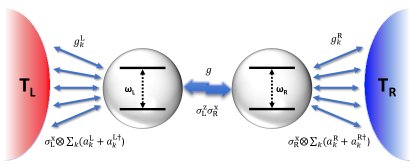
Figure 1: (Color online) Schematic diagram of the quantum thermal diode based on two qubits coupled via anisotropic (Raman-induced) spin-spin interaction $\hat{\sigma}_{\text{L}}^{z}\hat{\sigma}_{\text{R}}^{x}$. The left qubit has transition frequency $\omega_{L}$ while right qubit has transition frequency $\omega_{R}$ and the coupling strength between the qubits is denoted by $g$. Each qubit is coupled with a thermal bath and we assume these baths are independent and may have any distinct non-negative temperatures.

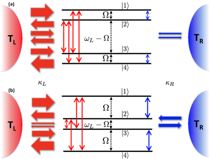
Figure 2: (Color online) Same systeme, but with the system Hamiltonian represented by a diagonalized form. The left bath induces transitions $1\leftrightarrow 3$, $2\leftrightarrow 3$, $1\leftrightarrow 4$ and $2\leftrightarrow 4$, whereas the right bath induces transitions $1\leftrightarrow 2$ and $3\leftrightarrow 4$. (a) Large coupling $g$, (b) small coupling $g$ for resonant qubits. In both cases the left bath is at a higher temperature than the right bath.

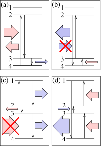
Figure 3: (Color online) Examples of processes that rectify heat current. Panels (a) and (b) correspond to small $g$, panels (c) and (d) to large $g$; panels (a) and (c) show the left bath is hotter than the right one, and in panels (b) and (d) it is vice versa. For small $g$, heat can flow from left to right, e.g., via the Raman cycle (4234) (a), whereas the opposite cycle (4324) (b) is inhibited because the cold reservoir cannot excite the $|3\rangle\to|2\rangle$ transition. For large $g$ and for temperatures of the hot reservoir that can not excite $|4\rangle\to|1\rangle$ transition, the four-wave mixing cycle (41234) (c) may not be achieved , whereas the opposite cycle (43214) (d) can conduct heat from right to left.

The rectification effect can be explained by considering possible cycles between the four states $|1\rangle,|2\rangle,|3\rangle,|4\rangle$ which transmit heat from the hot to the cold reservoir via global channels. In principle, there are three possible Raman cycles (3213), (4214), (4234), and their inverses [here (3213) means the sequence of transitions $|3\rangle\to|2\rangle\to|1\rangle\to|3\rangle$, etc.]. In addition, three four-wave mixing cycles (41234), (43124), (41324), and their inverses are also possible. Among the four-wave mixing cycles, only the global cycle (41234) transfers heat between the reservoirs while the remaining two keep the energies of the reservoirs unchanged. Depending on the bath temperatures, some cycles can be inhibited in one direction because the reservoir cannot provide photons of sufficient energy to excite particular transitions. As an example, consider the Raman cycle (4234) for small $g$ as shown in Figs. 3(a) and 3(b). If the left bath is hot, i.e., $T_{\text{L}}>T_{\text{R}}$ (Fig. 3(a)) the cycle may be completed. However, if $T_{\text{R}}>T_{\text{L}}$ (Fig. 3(b)) then left bath can not excite the $|3\rangle\to|2\rangle$ transition, consequently the heat transfer from right to left is inhibited and the device rectifies heat from left to right.

As another example, consider the four-wave mixing cycle (41234) for large $g$ as shown in Figs. 3(c) and 3(d). If the left bath is hot (Fig. 3(c)) but not hot enough to excite the $|4\rangle\to|1\rangle$ transition, the heat transfer from the left to the right bath is inhibited. On the contrary, if the right bath is hot (Fig. 3(d)) the reverse cycle may be completed without obstruction so that the device rectifies from right to left.

The proposed mechanism of the non-reciprocal heat transport relies neither on the frequency difference of the qubits nor on the asymmetry of the dissipation rates of the baths. In our model high rectification can be obtained even for resonant qubits with symmetric couplings to their reservoirs. This is in contrast to other diode models that rely on asymmetric qubit-bath couplings and difference in qubit frequencies to attain rectification  Man et al. (2016); Ordonez-Miranda et al. (2017).

III Heat Currents and Rectification Factor

In order to characterize the heat flow in our system, we calculate the heat currents $\mathcal{J}_{\text{R}}$ and $\mathcal{J}_{\text{L}}$ from the two baths. According to the definition Alicki and Kosloff (2018) we have

$$\mathcal{J}_{\text{R}}=\text{Tr}[\hat{\mathcal{L}}_{\text{R}}\hat{\tilde{H}}].$$ (4)

The first law of thermodynamics requires that at steady state the heat currents satisfy $\mathcal{J}_{\text{R}}=-\mathcal{J}_{\text{L}}$ (a positive value of the heat current indicates heat flowing from the bath into the system). Here, we only report $\mathcal{J}_{\text{R}}$ and relation for $\mathcal{J}_{\text{L}}$ is given in Appendix C. Using Eq. (3) in Eq. (4) the heat current from the right bath is

$$\mathcal{J}_{\text{R}}=-\frac{1}{2}\kappa_{\text{R}}\Omega\cos^{2}\theta[1+(2\bar{n}_{\text{R}}+1)(\cos\theta\langle\hat{\sigma}_{\text{R}}^{z}\rangle+\sin\theta\langle\hat{\sigma}_{\text{L}}^{z}\hat{\sigma}_{\text{R}}^{x}\rangle)].$$ (5)

Out of the heat currents one can calculate the rectification factor Li et al. (2012),

$$\mathcal{R}=\frac{\left|\mathcal{J}_{\text{R}}(T_{\text{R}},T_{\text{L}})+\mathcal{J}_{\text{R}}(T_{\text{L}},T_{\text{R}})\right|}{\text{Max}(\left|\mathcal{J}_{\text{R}}(T_{\text{R}},T_{\text{L}})\right|,\left|\mathcal{J}_{\text{R}}(T_{\text{L}},T_{\text{R}}))\right|},$$ (6)

where the $\mathcal{J}_{\text{R}}(T_{\text{R}},T_{\text{L}})$ is the heat current from the right bath into the system for $T_{\text{R}}>T_{\text{L}}$, and vice versa for $\mathcal{J}_{\text{R}}(T_{\text{L}},T_{\text{R}})$ and $T_{\text{L}}>T_{\text{R}}$. The rectification factor is a figure of merit that measures the quality of the diode, taking values between 0 (symmetric heat flow) and 1 (perfect diode).

In our numerical calculations we consider resonant (RQ, $\omega_{L}=\omega_{R}$) and off-resonant (ORQ, $\omega_{L}\neq\omega_{R}$) qubits for both Ohmic (OSD) and flat (FSD) spectral densities of the baths. The simulations are done using scientific python packages along with key libraries from QuTiP Johansson et al. (2013).

III.1 Effects of Asymmetric Exchange Interaction Strength

With ORQs, unit rectification is possible for wide range of system parameters. However, here we consider resonant case to show that unit rectifications is also possible for RQs. Note that in thermal diode models proposed in Werlang et al. (2014); Man et al. (2016); Ordonez-Miranda et al. (2017), rectification is not possible for RQs when each qubit is connected to a separate thermal bath.

In Fig. 4 we plot the heat current $\mathcal{J}_{\text{R}}$ and the rectification factor $\mathcal{R}$ for different values of $T_{\text{L}}$ and $T_{\text{R}}$ with RQs and baths with FSD. As can be seen, the heat flow is asymmetric with respect to the $T_{\text{L}}=T_{\text{R}}$ axis (Figs. 4(a) and 4(b)): For $T_{\text{R}}>T_{\text{L}}$, the heat current $\left|\mathcal{J}_{\text{R}}\right|$ is smaller compared to the case when thermal biased is reversed so that the system rectifies heat from left to right. Although rectification is stronger for off-resonant qubits than for resonant, RQs bring crucial advantage of much larger heat flows. For example, the heat current for RQs is two orders of magnitude larger in comparison to that of ORQs with $\omega_{L}=20\omega_{R}$ and the same set of remaining parameters.

Figure 4: (Color online) Steady state heat current $\mathcal{J}_{\text{R}}$ and rectification $\mathcal{R}$ as functions of temperatures $T_{\text{L}}$ and $T_{\text{R}}$, assuming heat baths with FSD. The interaction strength is $g=0.01$ in the left and $g=1$ in the right column. Panels (a) and (b) show $\mathcal{J}_{\text{R}}$, and panels (c) and (d) show the corresponding values of $\mathcal{R}$. The qubits are resonant with $\omega_{\text{L}}=\omega_{\text{R}}=1$, and the dissipation rates are $\kappa_{\text{LL}}=\kappa_{\text{RR}}=0.01$.

Temperature dependence of the rectification factor for two different values of the qubit-qubit coupling strength $g$ is shown in Fig. 4(c) and 4(d). Almost perfect diode behavior for $g=0.01$ is obtained only with large temperature difference $\left|T_{\text{R}}-T_{\text{L}}\right|$ as shown in the Fig. 4(c), and $60\%$ rectification is possible over wide range of bath temperatures if coupling strength is increased to $g=1$ as shown in Fig. 4(d).

Our calculations show similar properties also for baths with OSD. However, the temperature domain of high rectification is then larger, while the heat current is reduced compared to the baths with FSD. This is related to the asymmetry of the spectrum and the proportionality of the spectral response functions to the transition frequencies.

III.2 Variation of Qubit Frequencies

Figure 5: (Color online) Rectification $\mathcal{R}$ as a function of the qubit frequencies $\omega_{\text{L}}$ and $\omega_{\text{R}}$. The interaction strength is $g=0.5$ in the left and $g=1$ in the right column. In panels (a) and (b) $T_{\text{R}}=0.5T_{\text{L}}=1$, and in panels (c) and (d) $T_{\text{R}}=0.05T_{\text{L}}=10$. The remaining parameters are the same as in Fig. 4.

In the previous subsection, we showed that the RQs behave as a thermal diode, and both quantitative and qualitative behaviors of rectification depends on coupling strength $g$. Other control parameters for rectification in our model are tuning the qubit frequencies and/or qubit-bath coupling rates $\kappa_{\text{ij}}$, where $i,j=\text{L,R}$ baths. Let us now analyze the effect of variation of qubits frequencies on the rectification magnitude. Fig. 5 shows $\mathcal{R}$ for two different coupling strengths, $g=0.01$ in the left column and $g=1$ in the right column. Figs. 5(a) and 5(b) are for small temperature difference between the two baths, while Figs. 5(c) and 5(d) correspond to large temperature differences. As can be seen, large temperature difference increases the diode quality irrespective of the strength of the qubit-qubit coupling. However, RQs generate vanishing rectification for small value of coupling strength $g=0.01$ as depicted in Fig. 5(c). On the other hand, almost unit rectification of the heat current by RQs can be obtained if the coupling strength is increased to $g=1$ (Fig. 5(d)). All these results demonstrate that the diode quality can be controlled in a wide range of system parameters. For instance, as shown in Fig. 4(c), RQs model with $g=0.01$ behaves as a thermal diode for a narrow range of temperature values, however this region can be enhanced by changing the qubit frequencies as shown in Fig. 5. System-bath coupling rates are another control parameter for the rectification, but here we consider them to be symmetric. A brief discussion to show the effect of dissipation rates on rectification is presented in the Appendix B.

IV Physical Model Systems for Possible Implementations

Asymmetric spin-spin interactions, such as $\sigma_{L}^{z}\sigma_{R}^{x}$, can be found in natural systems, for example, effectively in magnetic macromolecules in nuclear spin environments Tupitsyn et al. (1997) or directly in weak ferromagnetic systems with spin-orbit coupling Moriya (1960); Dzyaloshinsky (1958). More recently similar spin bath models are used to explore controlling dephasing of a single qubit Bhaktavatsala Rao and Kurizki (2011). Our HD mechanism rely on such an interaction between two qubits. We specifically use the same interaction ($\sigma_{L}^{z}\sigma_{R}^{x}$) proposed in Ref. Bernád and Torres (2015); where the model is motivated for its mathematical similarity to optomechanical coupling but no physical motivation or an implementation scheme is given. In order to produce such an interaction in a physical and controllable manner, we have suggested several systems in preceding sections. Here we will provide more details of these systems by presenting explicit model Hamiltonians.

IV.1 Optomechanical route for $\sigma_{L}^{z}\sigma_{R}^{x}$

The optomechanical coupling between an optical resonator of frequency $\omega$ and a mechanical resonator of frequency $\Omega$ can be written as Law (1994, 1995) ($\hbar=1$)

$$H=\omega a^{\dagger}a+\Omega b^{\dagger}b+ga^{\dagger}a(b+b^{\dagger}),$$ (7)

where the annihilation and creation operators of photons and phonons are denoted by $a,a^{\dagger}$ and $b,b^{\dagger}$, respectively. A statistical mutation of bosonic operators to spin operators can be constructed as an inversion of spin to boson Holstein-Primakoff transformation such that Carneiro and Pellegrino (2017)

$$a^{\dagger}a = J\mathds{1}+J_{z},\quad a=\frac{1}{\sqrt{J\mathds{1}+J_{z}}}J_{-},$$

$$a^{\dagger} = J_{+}\frac{1}{\sqrt{J\mathds{1}+J_{z}}},$$ (8)

where $J$ is the total spin and $J_{\pm},J_{z}$ satisfy the SU(2) algebra. Employing this transformation to both photons and phonons, and assuming weakly excited spins ($\langle J_{z}\rangle\ll J$) the bosonic optomechanical model can be mapped to the asymmetric spin-spin coupling model. We remark that replacing bosonic mechanical mode by a single spin-$1/2$ is employed in a circular quantum walk problem by assuming $\langle b^{d}agb\rangle\ll 1$ so that only the two lowest vibronic modes are accessible Moqadam and Portugal (2015).

The weak excitation condition as well as lack of physical qubits make the optomechanical route is a limited and indirect approach to implement our HD scheme. The other restrictions such as weak $g$ or frequency difference of optical and mechanical modes can be relaxed in electrical analogs of optomechanical-like couplings Johansson et al. (2014).

IV.2 Coupled Raman model route for $\sigma_{L}^{z}\sigma_{R}^{x}$

Hamiltonian of a system consisting of a three-level atom in a single mode cavity is given by ($\hbar=1$)

$$H = \omega a^{\dagger}a+\omega_{r}|r\rangle\langle r|+\omega_{e}|e\rangle\langle e|+\omega_{g}|g\rangle\langle g|+$$ (9)

$$+ g(a^{\dagger}(|g\rangle\langle r|+|e\rangle\langle r|)+\text{H.c.},$$

where $g$ is the cavity-atom coupling coefficient. $\omega_{r},\omega_{e},\omega_{g}$ denote the upper, middle, and lowest energy levels with the associated states $|r\rangle,|e\rangle,|g\rangle$, respectively. Assuming the lower doublet of energy levels are quasi-degenerate ($\omega_{e}\approx\omega_{r}$ and taking the detuning $\delta=\omega_{r}-\omega_{e}-\omega_{a}$ of the cavity mode from the atomic resonance is much greater than $g$ then the upper level can be adiabatically eliminated from the dynamics, which can be described by an effective Hamiltonian of the form

$$H=\omega_{c}a^{\dagger}a+\epsilon\sigma_{z}-\frac{g^{2}}{\delta}a^{\dagger}a\sigma_{x}.$$ (10)

This special two-photon transition model is known as the Raman coupled model Knight (1986); Phoenix and Knight (1990). Here, the intensity dependent Stark shift in the cavity frequency is neglected; we introduced $\epsilon=\omega_{e}-\omega_{g}$; and $\sigma_{z}=|e\rangle\langle e|-|g\rangle\langle g|,\sigma_{x}=|e\rangle\langle g|+|g\rangle\langle e|$. Similar to the optomechanical case, one can assume weak excitation of the cavity mode and replace $a^{\dagger}a$ with $\sigma_{L}^{z}$ to get the desired asymmetric spin-spin interaction effectively.

We remark that the Raman route is quite generic provided that we assume only two vibronic levels are involved in an optical Raman scattering from a molecule. The Raman scattering of a field $E$ is described by the interaction $q|E|^{2}$ where $q$ is the vibrational displacement which can be replaced by $\sigma_{x}$ in the case of two-level approximation for the vibrational motion. Using $E\sim(a+a^{\dagger})$ and neglecting two photon terms, $a^{\dagger}a\sigma_{x}$ is obtained Schoendorff and Risken (1990).

IV.3 Quantum walk with trapped ions scheme for $\sigma_{L}^{z}\sigma_{R}^{x}$

The quantum walk on a circle can be simulated with trapped ions where the steps of the walker are taken in quantum optical phase space according to the single step generator Travaglione and Milburn (2002)

$$U=\text{e}^{ip\sigma_{z}}H,$$ (11)

where $p$ is the momentum operator generating the step conditioned by the result of the coin toss operation. Here $H$ stands for the Hadamard gate operator. It is proposed that the step can be implemented using four Raman beam pulses sequentially Travaglione and Milburn (2002). Assuming steps are small such that vibrational excitation is much less than $1$ then again the effective Hamiltonian associated with the step generator corresponds to asymmetric spin-spin interaction $\sigma_{L}^{z}\sigma_{R}^{x}$.

IV.4 Circuit QED scheme for $\sigma_{L}^{z}\sigma_{R}^{x}$

General Hamiltonian of a superconducting resonator interacting with superconducting qubit can be expressed as Blais et al. (2004)

$$H=\omega a^{\dagger}a+\frac{\Omega}{2}+g(\cos{\theta}\sigma_{z}+\sin{\theta}\sigma_{x})(a+a^{\dagger}),$$ (12)

where $\omega$ is the frequency of the resonator with the annihilation and creation operators $a$ and ^†, respectively. The qubit frequency is denoted by $\Omega$. The coupling coefficient $g$ and the mixing angle $\theta$ depend on Josephson-Junction properties. By adjusting the junction parameters to get $\theta=0$ one gets the so called phase-gate term Blais et al. (2007), which becomes $\sigma_{L}^{z}\sigma_{R}^{x}$ if the resonator is weakly excited.

IV.5 Two-qubit Raman coupled scheme for $\sigma_{L}^{z}\sigma_{R}^{x}$

So far we have considered effective qubit systems to implement $\sigma_{L}^{z}\sigma_{R}^{x}$ coupling. Let us now assume a pair of three level atoms, each held separately in two bi-modal optical cavities. The cavities are coupled to each other via single-mode fibers as depicted in Fig. 6. This scheme is a generalization of the one for single-mode cavities described in Ref. Zheng et al. (2010). We consider the general case where the atomic transitions are driven by both classical laser and cavity fields. The interaction picture Hamiltonian describing the coupling of atoms and lasers is ($\hbar=1$)

$$H_{1}=\sum_{k=L,R}\sum_{x=e,g}\Omega_{kx}\text{e}^{i\Delta_{kx}t}|r_{k}\rangle\langle x_{k}|+\text{H.c.},$$ (13)

where $\Omega_{kx}$ is the Rabi frequency associated with the transition $|r_{k}\rangle\leftrightarrow|x_{k}\rangle$ and $\Delta_{kx}$ denotes the detuning of the laser from the respective transition. Similarly, interaction of the cavity modes and the atoms are expressed in the interaction picture as

$$H_{2}=\sum_{k=L,R}\sum_{x=e,g}g_{kx}a_{kx}\text{e}^{i\delta_{x}t}|r_{k}\rangle\langle x_{k}|+\text{H.c.}.$$ (14)

Here, $a_{kx}$ and $a_{kx}^{\dagger}$ are the annihilation and creation operators for the respective cavity modes and $\delta_{x}$ is the cavity detuning from the respective transition. The cavities are assumed to be connected to each other through single-mode (short) fibers. The optical interactions are described by the Hamiltonian

$$H_{3}=\sum_{e,g}\nu_{x}b_{x}(a_{Lx}^{\dagger}+a_{Rx}^{\dagger})+\text{H.c.},$$ (15)

where $g_{kx}$ is the atom-cavity coupling coefficient, $\nu_{x}$ is the coupling strength of the fiber mode and the respective cavity mode. Creation and annihilation operators for the fiber modes are denoted by $b_{x}$ and $b_{x}^{\dagger}$, respectively. The notation is shown in Fig. 7 for clarity. We remark that these Hamiltonians are straightforward direct generalization of those in Ref. Zheng et al. (2010). The only new ingredient here is that we allow for an additional classical drive and a cavity field acting on each atom such that each transition can be driven by both classical and cavity fields.

The full Raman coupled model allows us to engineer a variety of qubit-qubit interactions, including asymmetric ones. In particular we can generalize the example given in Ref. Zheng et al. (2010), where it is shown that if both the classical and cavity fields are driving only the $|r\rangle\leftrightarrow|g\rangle$ transition then the qubit-qubit interaction would of the form $\sim|g_{L}\rangle\langle g_{L}|\otimes|g_{R}\rangle\langle g_{R}|$. In our general case we can assume the similar situation for only one qubit such that $|r_{L}\rangle\leftrightarrow|g_{L}\rangle$ is driven by both the classical and cavity fields. While in the second qubit, we assume classical field drives the $|r_{R}\rangle\leftrightarrow|g_{R}\rangle$ and cavity field drives the $|r_{R}\rangle\leftrightarrow|e_{R}\rangle$ transition. The scheme is depicted in Fig. 7. Accordingly, this would yield an effective qubit-qubit coupling $|e_{L}\rangle\langle e_{L}|\otimes|g_{R}\rangle\langle e_{R}|$ that depends on the population of the $|e_{L}\rangle$. Taking into account the Hermitian conjugate process and expressing the coupling in terms of the Pauli spin operators we get the $\sigma_{L}^{z}\sigma_{R}^{x}$ interaction.

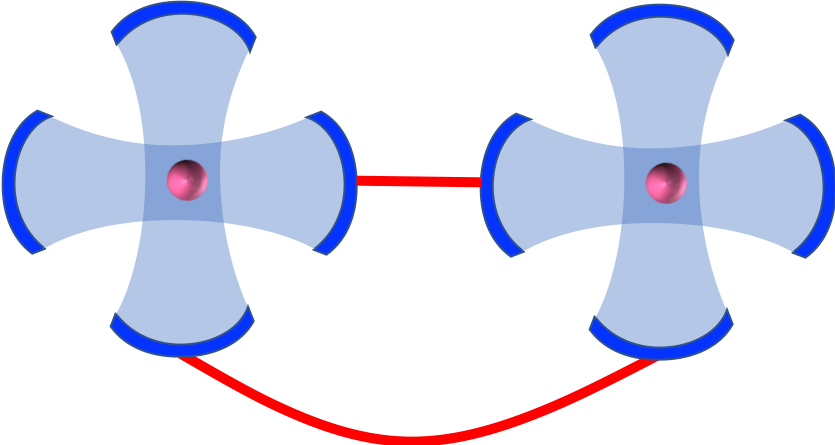
Figure 6: (Color online) Schematic diagram of two distant three-level atoms trapped inside fiber coupled bi-modal cavities.

Figure 7: (Color online) (Left panel) The classical laser and cavity field driven transitions in the three-level atoms, distinguished by label $x=L,R$ for the atom trapped in the left or right cavity (cf. Fig. 6). Both the classical and cavity fields drive the transitions. Upper, middle, and lower atomic states are denoted by $|r_{x}\rangle,|e_{x}\rangle$, and $g_{x}\rangle$, respectively. (Right panel) Special case where only the $|r_{L}\rangle\leftrightarrow|e_{L}\rangle$ is driven by the both classical laser and the cavity field. The other fields on the left atom are turned off. The right atom is driven by a single classical and a single cavity field in Raman configuration.

V Conclusion

We have investigated a quantum thermal diode composed of two qubits coupled to each other via anisotropic exchange interaction originally introduced in Ref. Bernád and Torres (2015). By deriving the global master equation, analytical expressions for the heat currents in the system are found. We have used the rectification factor to quantify the diode quality, calculating the results for both FSD and OSD of the thermal reservoirs. The rectification mechanism is explained in terms of the anisotropic exchange interactions: the baths can excite only some of the transitions in the Raman or four-wave-mixing global cycles so that some global cycles can run only in one direction and not oppositely. We have shown that in our model the diode behavior relies neither on the asymmetry of qubit frequencies nor on the difference of dissipation rates of the heat baths. Rectification can be achieved even for resonant qubits thus allowing to conduct large heat currents without compromising rectification efficiency. Since the anisotropic exchange model can be applied to natural weak ferromagnets Moriya (1960); Dzyaloshinsky (1958), nuclear spin environments Bhaktavatsala Rao and Kurizki (2011); Tupitsyn et al. (1997), cavity QED Knight (1986); Schoendorff and Risken (1990); Phoenix and Knight (1990), circuit QED Johansson et al. (2014); Blais et al. (2004, 2007); Zheng et al. (2010), trapped ions Travaglione and Milburn (2002), optomechanical systems Bernád and Torres (2015); Moqadam and Portugal (2015); Johansson et al. (2014) we anticipate that our results can be significant for the heat management in such systems.

VI acknowledgments

Ö. E. M acknowledges fruitful discussions with W. Niedenzu and R. Uzdin. C. K. thanks to hospitality of QUB-CTAMOP and Reykjavik University Nanophysics groups where some part of this work had been completed. C. K.  thanks to M. Paternostro, A. Manolescu, and N. Aral for useful discussions. Ö. E. M and C. K. acknowledges support from the Koç University TÜPRAŞ Energy Center (KUTEM). T.O. acknowledges support of the Czech Science Foundation (GAČR), grant 17-20479S. G.K acknowledges the support of DFG, ISF and SAERI.

Appendix A Global Master equation

We present the derivation of global master equation given in Eq. (3). The system Hamiltonian is diagonalized using the unitary transformation

$$U:=\exp\Big{(}-i\frac{\theta}{2}\hat{\sigma}_{\text{L}}^{z}\hat{\sigma}_{\text{R}}^{y}\Big{)},$$ (16)

where the angle $\theta$ is defined as

$$\sin\theta:=\frac{2g}{\Omega},\qquad\cos\theta:=\frac{\omega_{\text{R}}}{\Omega},\qquad\tan\theta:=\frac{2g}{\omega_{\text{R}}},$$ (17)

such that $\Omega:=\sqrt{\omega^{2}_{\text{R}}+4g^{2}}$. The transformed operators then read

$$\hat{\tilde{\sigma}}_{\text{L}}^{x} = U\hat{\sigma}_{\text{L}}^{x}U^{\dagger}=\cos\theta\hat{\sigma}_{\text{L}}^{x}+\sin\theta\hat{\sigma}_{\text{L}}^{y}\hat{\sigma}_{\text{R}}^{y},$$ (18)

$$\hat{\tilde{\sigma}}_{\text{L}}^{y} = U\hat{\sigma}_{\text{L}}^{y}U^{\dagger}=\cos\theta\hat{\sigma}_{\text{L}}^{y}-\sin\theta\hat{\sigma}_{\text{L}}^{x}\hat{\sigma}_{\text{R}}^{y},$$ (19)

$$\hat{\tilde{\sigma}}_{\text{L}}^{z} = U\hat{\sigma}_{\text{L}}^{z}U^{\dagger}={\sigma}_{\text{L}}^{z},$$ (20)

and

$$\hat{\tilde{\sigma}}_{\text{R}}^{x} = U\hat{\sigma}_{\text{R}}^{x}U^{\dagger}=\cos\theta\hat{\sigma}_{\text{R}}^{x}-\sin\theta\hat{\sigma}_{\text{L}}^{z}\hat{\sigma}_{\text{R}}^{z},$$ (21)

$$\hat{\tilde{\sigma}}_{\text{R}}^{y} = U\hat{\sigma}_{\text{R}}^{y}U^{\dagger}={\sigma}_{\text{R}}^{y},$$ (22)

$$\hat{\tilde{\sigma}}_{\text{R}}^{z} = U\hat{\sigma}_{\text{R}}^{z}U^{\dagger}=\cos\theta\hat{\sigma}_{\text{R}}^{z}-\sin\theta\hat{\sigma}_{\text{L}}^{z}\hat{\sigma}_{\text{R}}^{x}.$$ (23)

The back transformations from dressed operators to bare operators reads from the Eqs. (18)-(23) by switching dressed operators to bare operators and vice versa with $\theta$ replaced by $-\theta$. Then, with the transformation Eq. (16), the Hamiltonian in Eq. (1) is diagonalized to the Hamiltonian given in Eq. (2).

Eigenstates of the dressed Hamiltonian are given by the individual eigenstates of the qubits as,

$$\ket{1}=\cos\frac{\theta}{2}\ket{++}-\sin\frac{\theta}{2}\ket{+-}$$ (24)

$$\ket{2}=\sin\frac{\theta}{2}\ket{++}+\cos\frac{\theta}{2}\ket{+-}$$ (25)

$$\ket{3}=\cos\frac{\theta}{2}\ket{-+}+\sin\frac{\theta}{2}\ket{--}$$ (26)

$$\ket{4}=\cos\frac{\theta}{2}\ket{--}-\sin\frac{\theta}{2}\ket{-+},$$ (27)

with their corresponding eigenvalues $\omega_{1}=\frac{1}{2}(\omega_{\text{L}}+\Omega)$, $\omega_{2}=\frac{1}{2}(\omega_{\text{L}}-\Omega)$, $\omega_{3}=\frac{1}{2}(-\omega_{\text{L}}+\Omega)$, and $\omega_{4}=\frac{1}{2}(-\omega_{\text{L}}-\Omega)$, respectively.

The qubits are coupled to two baths of temperature $T_{\text{R}}$ and $T_{\text{L}}$ via the the Hamiltonian $\hat{H}_{SB}^{ij}=\hat{\sigma}_{i}^{x}\otimes\sum_{k}g_{k}^{j}(\hat{a}_{k}^{j}+\hat{a}_{k}^{j\dagger})$, where $g_{k}^{j}$ are the coupling strengths to baths, and $\hat{a}_{k}^{j}$ ($\hat{a}_{k}^{j\dagger}$) are the creation (annihilation) operator of the $k$ mode of the bath $i,j=\text{L,R}$, whose Hamiltonian is $\hat{H}_{j}=\sum_{k}\omega_{k}\hat{a}_{k}^{j\dagger}\hat{a}_{k}^{j}$. To calculate the master equation, we move to the interaction picture in which

$$\hat{\sigma}_{\text{L}}^{x}(t) = \cos\theta\hat{\tilde{\sigma}}_{\text{L}}^{-}e^{-i\omega_{\text{L}}t}-\sin\theta\hat{\tilde{\sigma}}_{\text{L}}^{+}\hat{\tilde{\sigma}}_{\text{R}}^{-}e^{-i(\Omega-\omega_{\text{L}})t}$$

$$+\sin\theta\hat{\tilde{\sigma}}_{\text{L}}^{-}\hat{\tilde{\sigma}}_{\text{R}}^{-}e^{-i(\Omega+\omega_{\text{L}})t}+\mathrm{H.c.}$$

$$\hat{\sigma}_{\text{R}}^{x}(t) = \cos\theta\hat{\tilde{\sigma}}_{\text{R}}^{-}e^{-i\Omega t}+\frac{1}{2}\sin\theta\hat{\tilde{\sigma}}_{\text{L}}^{z}\hat{\tilde{\sigma}}_{\text{R}}^{z}+\mathrm{H.c.}$$ (29)

Hence, the master equation in the interaction picture is found to be the one that is given in Eq. (3), with

$$G_{ij}(\omega)=\begin{cases}\kappa_{ij}(\omega)[1+\bar{n}_{j}(\omega)],&\omega>0\\ \kappa_{ij}(\left|\omega\right|)\bar{n}_{j}(\left|\omega\right|),&\omega<0\\ 0,&\omega=0\end{cases},$$ (30)

where $\bar{n}_{j}(\omega):=1/(\exp{\omega/T_{j}}-1)$ is the average excitation number of $j=\text{L,R}$ baths. We define $\kappa_{ij}(\omega)$ as rates, which are independent of frequency for the flat spectrum, and $\kappa_{ij}(\omega)=\kappa_{ij}\omega$ for the Ohmic spectrum.

$$\hat{\mathcal{L}}_{\text{Lj}} = G_{\text{Lj}}(\omega_{\text{L}})\cos^{2}\theta\hat{\mathcal{D}}[\hat{\tilde{\sigma}}_{\text{L}}^{-}]+G_{\text{Lj}}(-\omega_{\text{L}})\cos^{2}\theta\hat{\mathcal{D}}[\hat{\tilde{\sigma}}_{\text{L}}^{+}]$$

$$+ G_{\text{Lj}}(\omega_{\text{23}})\sin^{2}\theta\hat{\mathcal{D}}[\hat{\tilde{\sigma}}_{\text{L}}^{-}\hat{\tilde{\sigma}}_{\text{R}}^{+}]+G_{\text{Lj}}(-\omega_{\text{23}})\sin^{2}\theta\hat{\mathcal{D}}[\hat{\tilde{\sigma}}_{\text{L}}^{+}\hat{\tilde{\sigma}}_{\text{R}}^{-}]$$

$$+ G_{\text{Lj}}(\omega_{\text{14}})\sin^{2}\theta\hat{\mathcal{D}}[\hat{\tilde{\sigma}}_{\text{L}}^{-}\hat{\tilde{\sigma}}_{\text{R}}^{-}]+G_{\text{Lj}}(-\omega_{\text{14}})\sin^{2}\theta\hat{\mathcal{D}}[\hat{\tilde{\sigma}}_{\text{L}}^{+}\hat{\tilde{\sigma}}_{\text{R}}^{+}],$$

$$\hat{\mathcal{L}}_{\text{Rj}} = G_{\text{Rj}}(\Omega)\cos^{2}\theta\hat{\mathcal{D}}[\hat{\tilde{\sigma}}_{\text{R}}^{-}]+G_{\text{Rj}}(-\Omega)\cos^{2}\theta\hat{\mathcal{D}}[\hat{\tilde{\sigma}}_{\text{R}}^{+}],,$$ (32)

where the first index represents left (L) or right (R) qubit, and the second index $j=\text{L,R}$ is for baths with $\theta=\arctan(2g/\omega_{\text{R}})$. In the main text, we consider $\kappa_{ij}=0$ for distinct $i$ and $j$. The Lindblad dissipators $\hat{\mathcal{D}}[\hat{A}]$ are defined as Lindblad (1976); Gorini et al. (1976)

$$\hat{\mathcal{D}}[\hat{A}]=\hat{A}\hat{\rho}\hat{A}^{\dagger}-\frac{1}{2}\left(\hat{A}^{\dagger}\hat{A}\hat{\rho}+\hat{\rho}\hat{A}^{\dagger}\hat{A}\right).$$ (33)

Appendix B Case of Spatially Overlapping Thermal Baths Over the Both Qubits

Figure 8: (Color online) Rectification $\mathcal{R}$ for the cases with different coupling rates between both baths to both qubits. Panel (a) shows the local bath case. Panels (b) and (c) show the case with both baths accessing their local qubits symmetrically but asymmetrically to the other one. Panel (c) is the case with all the qubit-bath couplings being symmetric. In all panels, $T_{\text{L}}=10$, $T_{\text{R}}=0.5$, and $\kappa_{\text{LL}}=\kappa_{\text{RR}}=0.01$. Rest of the parameters are the same as in Fig. 4.

In our treatment, we have assumed that each bath is only connected to its corresponding qubit. The assumption of local baths for the qubits however is restrictive for possible embodiments of our thermal diode scheme. In practice, thermal baths can overlap spatially over the closely spaced pair of interacting qubits. Special systems where such an overlap can be exactly absent could still be found. One scenario is to use optomechanical like coupling of two transmission line resonators as proposed in Ref. Johansson et al. (2014). If the resonators are weakly excited to the limit of a single photon, then the system mimics our case of two interacting qubits with local baths realized by using thermal noise currents fed into the transmission line resonators. For other implementations, such as using trapped ions Travaglione and Milburn (2002), off-resonant Raman systems Phoenix and Knight (1990), or asymmetric exchange interactions Moriya (1960); Dzyaloshinsky (1958), spatial overlap of the thermal baths can be unavoidable without taking additional measures such as using local modulation of the qubits by external drives to effectively make the baths local Gordon and Kurizki (2006, 2011). Apart from such extra design complications, we would like to now address the question to which extent spatial overlap of the baths over the qubit pair can be tolerated for a significant thermal rectification. For that aim, we consider a generalization of our master equation Eq. 3 by including the cross terms $\hat{\mathcal{L}}_{\text{LR}}$ and $\hat{\mathcal{L}}_{\text{RL}}$ describing the access of the non-local thermal baths to both qubits in the bare state picture.

Fig. 8(a) shows the case $\kappa_{\text{LR}}=\kappa_{\text{RL}}=0$, which is equivalent to local case given in Eq. 3. We have considered two cases, where the spatial overlap of the baths may lead to the same or different coupling rates to the distant qubits. In all cases, spatial overlap degrades the thermal diode quality by decreasing the maximum rectification factor. On the other hand, in the case of different coupling rates of the baths to their distant qubits we have found that the lowest value of the rectification factor is increased, as shown in Figs. 8(b) and 8(c). The decrease of the diode quality is severe in the case of same coupling rates of the baths to the distant qubits. When the cross-coupling rate is about half of the local coupling rate then the diode operates at half efficiency, where the rectification factor is reduced from $\sim 90\%$ to $\sim 45\%$. When all the coupling rates are equal to each other the rectification is practically lost.

We conclude that if the spatial overlap of the thermal baths cannot be avoided then either asymmetric coupling rates to distant qubits should be sought for or local modulators on qubits should be implemented Gordon and Kurizki (2006, 2011).

Appendix C Dynamics and the Heat Currents

Equations of motions for the relevant dynamical observables of our system are determined from the master equation, Eq. (3), and given by

$$\dfrac{d}{dt}\langle\hat{\tilde{\sigma}}^{z}_{\text{L}}\rangle = \cos^{2}\theta[G_{\text{L}}(-\omega_{\text{L}})\langle\mathds{A}\rangle-G_{\text{L}}(\omega_{\text{L}})\langle\mathds{B}\rangle]$$

$$+\frac{1}{2}\sin^{2}\theta[G_{\text{L}}(\omega_{\text{1}})\langle\mathds{A}\mathds{D}\rangle-G_{\text{L}}(-\omega_{\text{1}})\langle\mathds{B}\mathds{C}\rangle$$

$$+G_{\text{L}}(-\omega_{\text{2}})\langle\mathds{A}\mathds{C}\rangle-G_{\text{L}}(\omega_{\text{2}})\langle\mathds{B}\mathds{D}\rangle]$$

$$\dfrac{d}{dt}\langle\hat{\tilde{\sigma}}^{z}_{\text{R}}\rangle = \cos^{2}\theta[G_{\text{R}}(-\Omega)\langle\mathds{C}\rangle-G_{\text{R}}(\Omega)\langle\mathds{D}\rangle]$$

$$+\frac{1}{2}\sin^{2}\theta[-G_{\text{L}}(\omega_{\text{1}})\langle\mathds{A}\mathds{D}\rangle+G_{\text{L}}(-\omega_{\text{1}})\langle\mathds{B}\mathds{C}\rangle$$

$$+G_{\text{L}}(-\omega_{\text{2}})\langle\mathds{A}\mathds{C}\rangle-G_{\text{L}}(\omega_{\text{2}})\langle\mathds{B}\mathds{D}\rangle]$$

$$\dfrac{d}{dt}\langle\hat{\tilde{\sigma}}^{z}_{\text{L}}\hat{\tilde{\sigma}}^{z}_{\text{R}}\rangle = \cos^{2}\theta[G_{\text{L}}(-\omega_{\text{L}})\langle\mathds{A}\hat{\tilde{\sigma}}^{z}_{\text{R}}\rangle-G_{\text{L}}(\omega_{\text{L}})\langle\mathds{B}\hat{\tilde{\sigma}}^{z}_{\text{R}}\rangle$$ (36)

$$+G_{\text{R}}(-\Omega)\langle\mathds{D}\hat{\tilde{\sigma}}^{z}_{\text{L}}\rangle-G_{\text{R}}(\Omega)\langle\mathds{C}\hat{\tilde{\sigma}}^{z}_{\text{L}}\rangle],$$

where we introduce the operators $\mathds{A}=(\mathds{1}-\hat{\tilde{\sigma}}_{\text{L}}^{z})$, $\mathds{B}=(\mathds{1}+\hat{\tilde{\sigma}}_{\text{L}}^{z})$, $\mathds{C}=(\mathds{1}-\hat{\tilde{\sigma}}_{\text{R}}^{z})$, and $\mathds{D}=(\mathds{1}+\hat{\tilde{\sigma}}_{\text{R}}^{z})$.

The heat currents evaluate to

$$\mathcal{J}_{\text{L}} = \frac{1}{2}\omega_{\text{L}}\cos^{2}\theta[G_{\text{L}}(-\omega_{\text{L}})\langle\mathds{A}\rangle-G_{\text{L}}(\omega_{\text{L}})\langle\mathds{B}\rangle]$$

$$+ \frac{1}{4}\sin^{2}\theta[\omega_{\text{1}}G_{\text{L}}(-\omega_{\text{1}})\langle\mathds{B}\mathds{C}\rangle-\omega_{\text{1}}G_{\text{L}}(\omega_{\text{1}})\langle\mathds{A}\mathds{D}\rangle$$

$$- \omega_{\text{2}}G_{\text{L}}(\omega_{\text{2}})\langle\mathds{B}\mathds{D}\rangle+\omega_{\text{2}}G_{\text{L}}(-\omega_{\text{2}})\langle\mathds{A}\mathds{C}\rangle],$$

$$\mathcal{J}_{\text{R}} = \frac{1}{2}\Omega\cos^{2}\theta[G_{\text{R}}(-\Omega)\langle\mathds{C}\rangle-G_{\text{R}}(\Omega)\langle\mathds{D}\rangle].$$ (38)

Substitution of transformed operators relation given in Eq. (23) to Eq. (38) yields the heat current relation in terms of bare operators and given in Eq. (5). Even though, the Eqs. (C)-(38) are easy to solve, the analytical expressions are too cumbersome to report her. However, we confirmed that $\mathcal{J}_{\text{L}}+\mathcal{J}_{\text{R}}=0$ at the steady state.

References

- Giazotto et al. (2006) Francesco Giazotto, Tero T. Heikkila, Arttu Luukanen, Alexander M. Savin, and Jukka P. Pekola, “Opportunities for mesoscopics in thermometry and refrigeration: Physics and applications,” Rev. Mod. Phys. 78, 217–274 (2006).
- Roberts and Walker (2011) N.A. Roberts and D.G. Walker, “A review of thermal rectification observations and models in solid materials,” Int. J. Therm. Sci. 50, 648 – 662 (2011).
- Li et al. (2012) Nianbei Li, Jie Ren, Lei Wang, Gang Zhang, Peter Hanggi, and Baowen Li, “Colloquium: Phononics: Manipulating heat flow with electronic analogs and beyond,” Rev. Mod. Phys. 84, 1045–1066 (2012).
- Benenti et al. (2017) Giuliano Benenti, Giulio Casati, Keiji Saito, and Robert S. Whitney, “Fundamental aspects of steady-state conversion of heat to work at the nanoscale,” Phys. Rep. 694, 1 – 124 (2017).
- Terraneo et al. (2002) M. Terraneo, M. Peyrard, and G. Casati, “Controlling the energy flow in nonlinear lattices: A model for a thermal rectifier,” Phys. Rev. Lett. 88, 094302 (2002).
- Li et al. (2004) Baowen Li, Lei Wang, and Giulio Casati, Phys. Rev. Lett. 93, 184301 (2004).
- Lan and Li (2006) Jinghua Lan and Baowen Li, “Thermal rectifying effect in two-dimensional anharmonic lattices,” Phys. Rev. B 74, 214305 (2006).
- Lan and Li (2007) Jinghua Lan and Baowen Li, “Vibrational spectra and thermal rectification in three-dimensional anharmonic lattices,” Phys. Rev. B 75, 214302 (2007).
- Yang et al. (2007) Nuo Yang, Nianbei Li, Lei Wang, and Baowen Li, “Thermal rectification and negative differential thermal resistance in lattices with mass gradient,” Phys. Rev. B 76, 020301 (2007).
- Lo et al. (2008) Wei Chung Lo, Lei Wang, and Baowen Li, “Thermal transistor: Heat flux switching and modulating,” J. Phys. Soc. Jpn. 77, 054402 (2008).
- Chang et al. (2006) C. W. Chang, D. Okawa, A. Majumdar, and A. Zettl, “Solid-state thermal rectifier,” Science 314, 1121–1124 (2006).
- Li et al. (2006) Baowen Li, Lei Wang, and Giulio Casati, “Negative differential thermal resistance and thermal transistor,” Appl. Phys. Lett. 88, 143501 (2006).
- Hwang et al. (2009) J. Hwang, M. Pototschnig, R. Lettow, G. Zumofen, A. Renn, S. Götzinger, and V. Sandoghdar, “A single-molecule optical transistor,” Nature 460 (2009).
- Ordonez-Miranda et al. (2016) Jose Ordonez-Miranda, Younès Ezzahri, Jérémie Drevillon, and Karl Joulain, “Transistorlike device for heating and cooling based on the thermal hysteresis of ,” Phys. Rev. Appl. 6, 054003 (2016).
- Shen et al. (2011) Yuecheng Shen, Matthew Bradford, and Jung-Tsung Shen, “Single-photon diode by exploiting the photon polarization in a waveguide,” Phys. Rev. Lett. 107, 173902 (2011).
- Karimi et al. (2017) B Karimi, J P Pekola, M Campisi, and R Fazio, “Coupled qubits as a quantum heat switch,” Quantum Sci. Technol. 2, 044007 (2017).
- Ronzani et al. (2018) Alberto Ronzani, Bayan Karimi, Jorden Senior, Yu-Cheng Chang, Joonas T. Peltonen, ChiiDong Chen, and Jukka P. Pekola, “Tunable photonic heat transport in a quantum heat valve,” Nat. Phys. 14, 991–995 (2018).
- Barzanjeh et al. (2018) Shabir Barzanjeh, Matteo Aquilina, and André Xuereb, “Manipulating the flow of thermal noise in quantum devices,” Phys. Rev. Lett. 120, 060601 (2018).
- Ojanen and Jauho (2008) Teemu Ojanen and Antti-Pekka Jauho, “Mesoscopic photon heat transistor,” Phys. Rev. Lett. 100, 155902 (2008).
- Joulain et al. (2016) Karl Joulain, Jérémie Drevillon, Younès Ezzahri, and Jose Ordonez-Miranda, “Quantum thermal transistor,” Phys. Rev. Lett. 116, 200601 (2016).
- Landi et al. (2014) Gabriel T. Landi, E. Novais, Mário J. de Oliveira, and Dragi Karevski, “Flux rectification in the quantum xxz chain,” Phys. Rev. E 90, 042142 (2014).
- Werlang et al. (2014) T. Werlang, M. A. Marchiori, M. F. Cornelio, and D. Valente, “Optimal rectification in the ultrastrong coupling regime,” Phys. Rev. E 89, 062109 (2014).
- Man et al. (2016) Zhong-Xiao Man, Nguyen Ba An, and Yun-Jie Xia, “Controlling heat flows among three reservoirs asymmetrically coupled to two two-level systems,” Phys. Rev. E 94, 042135 (2016).
- Ordonez-Miranda et al. (2017) Jose Ordonez-Miranda, Younes Ezahri, and Karl Joulain, “Quantum thermal diode based on two interacting spinlike systems under different excitations,” Phys. Rev. E 95, 022128 (2017).
- Roche et al. (2015) B. Roche, P. Roulleau, T. Jullien, Y. Jompol, I. Farrer, D. A. Ritchie, and D. C. Glattli, “Harvesting dissipated energy with a mesoscopic ratchet,” Nat. Commun. 6 (2015).
- Thierschmann et al. (2015) Holger Thierschmann, Rafael Sánchez, Björn Sothmann, Fabian Arnold, Christian Heyn, Wolfgang Hansen, Hartmut Buhmann, and Laurens W. Molenkamp, “Three-terminal energy harvester with coupled quantum dots,” Nat. Nanotechnol. 10 (2015).
- Wang and Li (2007) Lei Wang and Baowen Li, “Thermal logic gates: Computation with phonons,” Phys. Rev. Lett. 99, 177208 (2007).
- Pfeffer et al. (2015) P. Pfeffer, F. Hartmann, S. Hofling, M. Kamp, and L. Worschech, “Logical stochastic resonance with a coulomb-coupled quantum-dot rectifier,” Phys. Rev. Appl. 4, 014011 (2015).
- Roßnagel et al. (2016) Johannes Roßnagel, Samuel T. Dawkins, Karl N. Tolazzi, Obinna Abah, Eric Lutz, Ferdinand Schmidt-Kaler, and Kilian Singer, “A single-atom heat engine,” Science 352, 325–329 (2016).
- Karimi and Pekola (2016) B. Karimi and J. P. Pekola, “Otto refrigerator based on a superconducting qubit: Classical and quantum performance,” Phys. Rev. B 94, 184503 (2016).
- Kouwenhoven et al. (1991) L. P. Kouwenhoven, A. T. Johnson, N. C. van der Vaart, C. J. P. M. Harmans, and C. T. Foxon, “Quantized current in a quantum-dot turnstile using oscillating tunnel barriers,” Phys. Rev. Lett. 67, 1626–1629 (1991).
- Moldoveanu et al. (2007) Valeriu Moldoveanu, Vidar Gudmundsson, and Andrei Manolescu, “Nonadiabatic transport in a quantum dot turnstile,” Phys. Rev. B 76, 165308 (2007).
- Gudmundsson et al. (2012) Vidar Gudmundsson, Olafur Jonasson, Chi-Shung Tang, Hsi-Sheng Goan, and Andrei Manolescu, “Time-dependent transport of electrons through a photon cavity,” Phys. Rev. B 85, 075306 (2012).
- Reimann et al. (1997) Peter Reimann, Milena Grifoni, and Peter Hänggi, “Quantum ratchets,” Phys. Rev. Lett. 79, 10–13 (1997).
- Casati and Mejia-Monasterio (2007) Giulio Casati and Carlos Mejia-Monasterio, “Heat flow in classical and quantum systems and thermal rectification,” AIP Conference Proceedings 965, 221–231 (2007).
- Vinitha Balachandran (2018) Emmanuel Pereira Giulio Casati Dario Poletti Vinitha Balachandran, Giuliano Benenti, “Heat current rectification in segmented xxz chains,” arXiv:1809.01917 (2018).
- Dames (2009) C. Dames, “Solid-State Thermal Rectification With Existing Bulk Materials,” J. Heat Transfer 131, 061301–061301–7 (2009).
- Maznev et al. (2013) A. A. Maznev, A. G. Every, and O. B. Wright, “Reciprocity in reflection and transmission: What is a ‘phonon diode’?” Wave Motion 50, 776–784 (2013).
- Jeżowski and Rafalowicz (1978) A. Jeżowski and J. Rafalowicz, “Heat flow asymmetry on a junction of quartz with graphite,” physica status solidi A 47, 229–232 (1978).
- Bhaktavatsala Rao and Kurizki (2011) D. D. Bhaktavatsala Rao and Gershon Kurizki, “From Zeno to anti-Zeno regime: Decoherence-control dependence on the quantum statistics of the bath,” Phys. Rev. A 83, 032105 (2011).
- Moriya (1960) Tôru Moriya, “Anisotropic Superexchange Interaction and Weak Ferromagnetism,” Phys. Rev. 120, 91–98 (1960).
- Dzyaloshinsky (1958) I. Dzyaloshinsky, “A thermodynamic theory of weak ferromagnetism of antiferromagnetics,” J. Phys. Chem. Solids 4, 241–255 (1958).
- Tupitsyn et al. (1997) I. S. Tupitsyn, N. V. Prokof’ev, and P. C. E. Stamp, “Effective Hamiltonian in the Problem of a "Central Spin" Coupled to a Spin Environment,” Int. J. Mod. Phys. B 11, 2901–2926 (1997).
- Knight (1986) P. L. Knight, “Quantum fluctuations and squeezing in the interaction of an atom with a single field mode,” Phys. Scri. 1986, 51 (1986).
- Schoendorff and Risken (1990) L. Schoendorff and H. Risken, “Analytic solution of the density-operator equation for the Raman-coupled model with cavity damping,” Phys. Rev. A 41, 5147–5155 (1990).
- Phoenix and Knight (1990) S. J. D. Phoenix and P. L. Knight, “Periodicity, phase, and entropy in models of two-photonresonance,” J. Opt. Soc. Am. B 7, 116–124 (1990).
- Travaglione and Milburn (2002) B. C. Travaglione and G. J. Milburn, “Implementing the quantum random walk,” Phys. Rev. A 65, 032310 (2002).
- Johansson et al. (2014) J. R. Johansson, G. Johansson, and Franco Nori, “Optomechanical-like coupling between superconducting resonators,” Phys. Rev. A 90, 053833 (2014).
- Blais et al. (2004) Alexandre Blais, Ren-Shou Huang, Andreas Wallraff, S. M. Girvin, and R. J. Schoelkopf, “Cavity quantum electrodynamics for superconducting electrical circuits: An architecture for quantum computation,” Phys. Rev. A 69, 062320 (2004).
- Blais et al. (2007) Alexandre Blais, Jay Gambetta, A. Wallraff, D. I. Schuster, S. M. Girvin, M. H. Devoret, and R. J. Schoelkopf, “Quantum-information processing with circuit quantum electrodynamics,” Phys. Rev. A 75, 032329 (2007).
- Zheng et al. (2010) Shi-Biao Zheng, Chui-Ping Yang, and Franco Nori, “Arbitrary control of coherent dynamics for distant qubits in a quantum network,” Phys. Rev. A 82, 042327 (2010).
- Bernád and Torres (2015) József Zsolt Bernád and Juan Mauricio Torres, “Partly invariant steady state of two interacting open quantum systems,” Phys. Rev. A 92, 062114 (2015).
- Law (1994) C. K. Law, “Effective Hamiltonian for the radiation in a cavity with a moving mirror and a time-varying dielectric medium,” Phys. Rev. A 49, 433–437 (1994).
- Law (1995) C. K. Law, “Interaction between a moving mirror and radiation pressure: A Hamiltonian formulation,” Phys. Rev. A 51, 2537–2541 (1995).
- Moqadam and Portugal (2015) J. K. Moqadam and R. Portugal, “Quantum walks on a circle with optomechanical systems,” Quantum Inform. Proc. 14 (2015).
- Breuer and Petruccione (2002) H. P. Breuer and F. Petruccione, The theory of open quantum systems (Oxford university press, 2002).
- Rivas et al. (2010) Angel Rivas, A Douglas K Plato, Susana F Huelga, and Martin B Plenio, “Markovian master equations: a critical study,” New J. Phys. 12, 113032 (2010).
- Hofer et al. (2017) P. P. Hofer, M. P. Llobet, D. M. Miranda, G. Haack, R. Silva, J. B. Brask, and N. Brunner, “Markovian master equations for quantum thermal machines: local versus global approach,” New. J. Phys. 19, 123037 (2017).
- Levy and Kosloff (2014) Amikam Levy and Ronnie Kosloff, “The local approach to quantum transport may violate the second law of thermodynamics,” EPL 107, 20004 (2014).
- Manrique et al. (2015) P. D. Manrique, F. Rodri-guez, L. Quiroga, and N. F. Johnson, “Nonequilibrium quantum systems: Divergence between global and local descriptions,” Adv. Condens. Matter Phys. 19, 615727 (2015).
- González et al. (2017) J. O. González, L. A. Correa, G. Nocerino, J. P. Palao, D. Alonso, and G. Adesso, “Testing the validity of the ‘local’ and ‘global’ gkls master equations on an exactly solvable model,” Open Syst. Inf. Dyn. 24, 1740010 (2017).
- Alicki and Kosloff (2018) R. Alicki and R. Kosloff, “Introduction to quantum thermodynamics: History and prospects,” arXiv:1801.08314 (2018).
- Johansson et al. (2013) J. Johansson, P. Nation, and F. Nori, “Qutip 2: A python framework for the dynamics of open quantum system,” Comput. Phys. Commun. 184 (2013).
- Carneiro and Pellegrino (2017) Carla Maria Pontes Carneiro and Giancarlo Queiroz Pellegrino, “Application of an inverse Holstein-Primakoff transformation to the Jaynes-Cummings model,” arXiv:1712.07589 (2017).
- Lindblad (1976) G. Lindblad, “On the generators of quantum dynamical semigroups,” Commun. math. Phys. 48 (1976).
- Gorini et al. (1976) V. Gorini, A. Kossakowski, and E. C. G. Sudarshan, “Completely positive dynamical semigroups of n level systems,” J. Math. Phys. 17 (1976).
- Gordon and Kurizki (2006) G. Gordon and G. Kurizki, “Preventing Multipartite Disentanglement by Local Modulations,” Phys. Rev. Lett. 97, 110503 (2006).
- Gordon and Kurizki (2011) Goren Gordon and Gershon Kurizki, “Scalability of decoherence control in entangled systems,” Phys. Rev. A 83, 032321 (2011).