The spectrum of a fast shock breakout from a stellar wind

Abstract

The breakout of a fast ($>0.1c$), yet sub-relativistic shock from a thick stellar wind is expected to produce a pulse of X-rays with a rise time of seconds to hours. Here, we construct a semi-analytic model for the breakout of a sub-relativistic, radiation-mediated shock from a thick stellar wind, and use it to compute the spectrum of the breakout emission. The model incorporates photon escape through the finite optical depth wind, assuming a diffusion approximation and a quasi-steady evolution of the shock structure during the breakout phase. We find that in sufficiently fast shocks, for which the breakout velocity exceeds about $0.1c$, the time-integrated spectrum of the breakout pulse is non-thermal, and the time-resolved temperature is expected to exhibit substantial decrease (roughly by one order of magnitude) during breakout, when the flux is still rising, because of the photon generation by the shock compression associated with the photon escape. We also derive a closure relation between the breakout duration, peak luminosity, and characteristic temperature that can be used to test whether an observed X-ray flare is consistent with being associated with a sub-relativistic shock breakout from a thick stellar wind or not. We also discuss implications of the spectral softening for a possible breakout event XRT 080109/SN 2008D.

1 Introduction

Radiation-mediated shocks (RMS) play a key role in shaping the early emission observed in various types of cosmic explosions. The radiation trapped inside the shock is released upon breakout of the shock from the thick envelope enshrouding the source of the explosion. The structure and velocity of the shock, and the characteristics of the consequent emission depend on the type of the progenitor, the explosion energy, and the angular extent of the ejecta (for a recent review see Waxman & Katz, 2017). While in certain situations the shock created in the explosion may become relativistic (Tan et al., 2001; Nakar & Sari, 2012; Kyutoku et al., 2014), in the majority of the events it is sub-relativistic, albeit fast.

In progenitors which are surrounded by sufficiently tenuous circumstellar medium, the breakout occurs as the shock approaches the sharp edge of the stellar envelope, whereupon it undergoes an abrupt transition from an RMS to a collisionless shock. However, if the progenitor is surrounded by a thick enough stellar wind, the shock continues to be radiation mediated also after it emerges from the stellar envelope and continues to propagate down the wind (Campana et al., 2006; Waxman et al., 2007; Soderberg et al., 2008; Katz et al., 2010; Balberg & Loeb, 2011). The shock physical width then increases during its propagation since the optical depth of the wind decreases.

In relativistic shocks, the breakout is significantly delayed, owing to opacity self-generation. It has been shown (Granot et al., 2018) that for a sufficiently high shock Lorentz factor $\gamma_{s}$, at which the immediate downstream temperature approaches $m_{e}c^{2}/3$, the transition to a collisionless shock occurs at a radius beyond which the (pair unloaded) Thomson optical depth to infinity ahead of the shock is $\tau\simeq m_{e}\gamma_{s}/m_{p}$. This is because beneath this radius, the number of escaping photons that are backscattered into the flow direction is larger than the number of electrons in the far upstream flow, giving rise to an accelerated pair production. In highly non-relativistic RMS, where pair production is negligible, the transition takes place once the optical depth ahead of the shock approaches $c/v_{s}$, where $v_{s}$ is the shock velocity. One might naively suspect that in the intermediate regime, specifically for shock velocities $v_{s}/c>\sqrt{m_{e}/m_{p}}$, pair production may become substantial, owing to a steepening of the shock or formation of a subshock that enhances the temperature. If true, it can lead to a delayed breakout as in the relativistic case. However, this can only happen if photon generation within a diffusion length is not efficient enough during the breakout. We show below that the temperature does not rise, or rather decreases, during the photon escape. In any event, once breakout commences and the radiative losses start increasing, the shock structure gradually changes, and this might affect the downstream temperature and the spectrum of emitted radiation. Thus, detailed calculations of the temperature profile during the breakout phase are desirable in order to address these issues. Such calculations can be performed using numerical methods, like the one developed by Ito et al. (2018). However, until this method will be adjusted to non-relativistic shocks, one may resort to an approximate analytic approach in order to get physical insight.

We note that a sub-relativistic shock breakout from a wind is expected for a smaller progenitor than a red supergiant star. Such a progenitor like a Wolf–Rayet (WR) star is known to eject winds before exploding as a Type Ic or Ib supernova (e.g., Tanaka et al., 2009; Gal-Yam et al., 2014). Although the shock breakout from a wind is recently observed to be common in Type II supernovae (e.g., Moriya et al., 2011; Ofek et al., 2014; Yaron et al., 2017; Forster et al., 2018), the candidates for sub-relativistic breakouts are still rare (Soderberg et al., 2008; Mazzali et al., 2008; Modjaz et al., 2009) because of its short, faint, and X-ray signal. Therefore, theoretical predictions are important for maximizing the observational prospects. A fast shock breakout may also happen in a binary neutron star merger like GW170817 (Abbott et al., 2017a; Abbott et al., 2017b) when a cocoon breaks out from the merger ejecta, and the breakout emission can dominate the jet emission (Kasliwal et al., 2017; Gottlieb et al., 2018; Nakar et al., 2018) because an off-axis jet is faint for a large viewing angle (Ioka & Nakamura, 2018).

At sufficiently low shock velocities, $v_{s}/c\ll 1$, the structure of an RMS can be computed analytically by employing the diffusion approximation. Such an approach has been undertaken by, e.g., Weaver (1976); Blandford & Payne (1981a, b); Katz et al. (2010). While Blandford & Payne (1981b) considered shocks in which photon advection by the upstream flow dominates over photon production, that might be suitable for gamma-ray burst outflows, Weaver (1976) and Katz et al. (2010) computed the structure of the RMS under conditions more suitable for shock breakout in stellar explosions. These studies indicate that the dominant photon source in such shocks is bremsstrahlung emission by the shocked electrons, and that once the shock velocity exceeds about $0.05c$ the radiation in the immediate shock downstream falls out of thermodynamic equilibrium and its temperature becomes extremely sensitive to the shock velocity: $T_{d}\propto v_{s}^{8}$. This strong dependence of temperature on velocity has important implications for the observational diagnostics of the breakout signal.

The analyses outlined above assume that the shock is infinite. However, as mentioned earlier, during the breakout phase an increasing fraction of the shock energy is radiated away, and the question arises as to what effect this might have on the structure and emission of the shock. Attempts to address this issue in case of a sudden breakout from a stellar envelope have been made recently using time-dependent models (Sapir et al., 2011; Katz et al., 2012; Sapir et al., 2013). Here, we consider a gradual breakout from a stellar wind. Under the assumption that the shock continuously adjusts to local conditions, so that it can be considered quasi-steady at any given time, we construct an analytic model that takes into account photon escape, and compute the temperature profile inside the shock for different values of the energy fraction escaping the system, by solving the photon transfer equation in the diffusion limit. The resultant temperature profiles are shown to be insensitive to the closure condition (e.g., angular distribution of the radiation) invoked upstream of the shock. We find that in fast shocks ($v/c\lower 2.15277pt\hbox{$\;\buildrel>\over{\sim}\;$}0.1$) the peak temperature decreases as the energy fraction escaping the shock increases. We also discuss the implications for the observed breakout signal, in particular to compare with a possible breakout event XRT 080109/SN 2008D.

2 Analytic model of the shock structure

Consider a sub-relativistic RMS propagating in the negative $x$-direction (${\bf v}=v\hat{x}$ in the shock frame). We suppose that in the frame of the shock the flow is stationary ($\partial_{t}=0$), and choose $x=0$ to be the boundary upstream from which photons escape to negative infinity, where the coordinate $x$ is measured in the shock frame. We further assume that the pressure is dominated by the radiation everywhere, and neglect the plasma pressure. In what follows, upstream quantities are labelled with a subscript $u$, whereby $v_{u}$, $n_{u}$, $n_{\gamma u}$, and $p_{\gamma u}$ are the velocity, plasma density, photon density, and radiation pressure in the far upstream flow, as measured in the shock frame. As will be confirmed, for the range of shock velocities considered below pair production can be ignored, hence the plasma density satisfies $n_{p}=n_{e}\equiv n$ everywhere.

In the diffusion limit, the photon number flux and radiation energy flux are given, to second order in $v_{u}/c$, by ${\bf j}_{\gamma}=j_{\gamma}\hat{x}$ and ${\bf f}_{\gamma}=f_{\gamma}\hat{x}$, respectively, with

$$j_{\gamma} = vn_{\gamma}-\frac{c}{3n\sigma_{T}}\frac{dn_{\gamma}}{dx},$$ (1)

$$f_{\gamma} = 4p_{\gamma}v-\frac{c}{n\sigma_{T}}\frac{dp_{\gamma}}{dx},$$ (2)

where $\sigma_{T}$ is the Thomson cross section (Blandford & Payne, 1981a, b). The fluid equations in the shock frame are reduced to:

$$m_{p}nv=m_{p}n_{u}v_{u} \equiv J,$$ (3)

$$\frac{d}{dx}(Jv+p_{\gamma}) = 0,$$ (4)

$$\frac{d}{dx}\left(Jv^{2}/2+f_{\gamma}\right) = 0.$$ (5)

The above equations can be rendered dimensionless upon defining $\tilde{p}_{\gamma}=p_{\gamma}/Jv_{u}$, $\tilde{v}=v/v_{u}$, and $d\tau^{\star}=(v_{u}/c)n_{e}\sigma_{T}dx$ (note that the velocity is included in the definition of the optical depth). Integrating Eqs. (4) and (5), using $\tilde{v}_{u}=1$, gives:

$$\tilde{v}+\tilde{p}_{\gamma} = 1+\tilde{p}_{\gamma u},$$ (6)

$$\frac{d\tilde{p}_{\gamma}}{d\tau^{\star}} = -\frac{1}{2}+\frac{1}{2}{\tilde{v}}^{2}+4\tilde{p}_{\gamma}{\tilde{v}}-\frac{1}{2}\tilde{f}_{\gamma u},$$ (7)

where

$$\tilde{f}_{\gamma u}=\frac{2f_{\gamma u}}{Jv_{u}^{2}}$$ (8)

denotes the fraction of shock energy that escapes to infinity, and must satisfy $\tilde{f}_{\gamma u}>-1$. Equations (6) and (7) admit an analytic solution for arbitrary values of $\tilde{p}_{\gamma u}$ and $\tilde{f}_{\gamma u}$:

$$\tilde{v}=\frac{4}{7}(1+\tilde{p}_{\gamma u})+\frac{\eta}{7}\tanh\left[\frac{\eta}{2}(\tau_{0}-\tau^{\star})\right],$$ (9)

where

$$\eta=\sqrt{(3-4\tilde{p}_{\gamma u})^{2}+56\tilde{p}_{\gamma u}-7\tilde{f}_{\gamma u}}$$ (10)

and

$$\tau_{0}=\frac{2}{\eta}\operatorname{arctanh}\left[\frac{3-4\tilde{p}_{\gamma u}}{\eta}\right]=\frac{1}{\eta}\ln\frac{\eta+3-4\tilde{p}_{\gamma u}}{\eta-3+4\tilde{p}_{\gamma u}},$$ (11)

for the boundary condition $\tilde{v}_{u}=1$ at $\tau^{\star}=0$. Here, $\tau_{0}$ is roughly the center of the shock transition layer (the precise location is slightly shifted, depending on the choice of parameters). It can be readily verified that the downstream velocity, $\tilde{v}_{d}=\tilde{v}(\tau^{\star}\rightarrow\infty)$, satisfies $\tilde{v}_{d}\geq 0$ for $\tilde{f}_{\gamma u}\geq-1$, and that no physical solutions exist for $\tilde{f}_{\gamma u}<-1$, as expected. It is also seen that with the choice $(d\tilde{p}_{\gamma}/d\tau^{\star})_{u}=0$, or $\tilde{f}_{\gamma u}=8\tilde{p}_{\gamma u}$ in our notation, which corresponds to an infinite shock with no escape, the solution obtained by Blandford & Payne (1981b) is recovered upon defining $\tau^{\star}-\tau_{0}\rightarrow\tau^{\star}$.

2.1 A note on boundary conditions

The solution described by Eq. (9) depends, formally, on two free parameters, $\tilde{p}_{\gamma u}$ and $\tilde{f}_{\gamma u}$. In an infinite shock with a cold upstream, the physical choice is $\tilde{p}_{\gamma u}=\tilde{f}_{\gamma u}=0$, since photons cannot reach distances larger than a few diffusion lengths upstream of the shock. In a finite shock with photon escape, the value of $\tilde{f}_{\gamma u}$ specifies the energy fraction which is radiated away. However, within the diffusion approximation the value of $\tilde{p}_{\gamma u}$ is uncertain, and there seems to be a degeneracy in the solution. In reality $\tilde{p}_{\gamma u}$ is fixed by additional physics beyond the diffusion approximation. One naively anticipates some relation of the form $f_{\gamma u}=e_{\gamma u}v_{rad}$, where $e_{\gamma u}$ is the energy density of the escaping radiation and $v_{rad}$ is some effective velocity that depends on the angular distribution of the radiation and, perhaps, some other details. If, for instance, one invokes complete beaming at the boundary $x=0$, then $e_{\gamma u}=p_{\gamma u}$, $v_{rad}=-c$, and $f_{\gamma u}=-p_{\gamma u}c$. In the other extreme, if the escaping radiation is taken to be sufficiently isotropic just upstream of the shock, then the effective velocity is $v_{rad}\simeq-v_{u}$, the equation of state is $e_{\gamma u}=3p_{\gamma u}$, and thus $f_{\gamma u}=-3p_{\gamma u}v_{u}$. In reality a similar relation likely holds, but with a somewhat different prefactor. We shall henceforth adopt the relation

$$\tilde{f}_{\gamma u}=-2\alpha\tilde{p}_{\gamma u},$$ (12)

and explore the dependence of the solution on the dimensionless parameter $\alpha$ (where a factor of $2$ comes from the normalization in Eq. (8)). Note that $\alpha=c/v_{u}$ for the complete beaming case and $\alpha=3$ for the isotropic case. To check the sensitivity of the solutions to the choice of $\alpha$, we examine a broader range of values, $1\leq\alpha\leq c/v_{u}$. In the above prescription $\alpha=1$ corresponds to a diffusion velocity $v_{rad}=-v_{u}/3$.

2.2 Shock solutions

Solutions for the shock profile are exhibited in Fig. 1 for $v_{u}/c=0.25$ and different values of $\tilde{f}_{\gamma u}$ and $\alpha$. As seen, photon escape leads to shock steepening, as expected. Specifically, for given values of $v_{u}$ and $n_{u}$, the shock transition layer becomes somewhat narrower as $\tilde{f}_{\gamma u}$ increases, and the far downstream velocity $v_{d}$ becomes smaller, giving rise to correspondingly larger values of the downstream density $n_{d}$, and somewhat larger values of the pressure $p_{\gamma d}$. Quite generally, the dependence of the solution on $\alpha$ is found to be rather weak (as long as the shock velocity is sub-relativistic i.e., $c/v_{u}\lower 2.15277pt\hbox{$\;\buildrel<\over{\sim}\;$}3$).

It is worth pointing out that, formally, as the fraction of shock energy which is radiated away approaches unity, namely $\tilde{f}_{\gamma u}=-1$, we have $\eta=4+2/\alpha$ compared with $\eta=3$ in the infinite case ($\tilde{f}_{\gamma u}=0$) with Eqs. (10) and (12). Since the width of the transition layer scales as $\sim 2/\eta$ (see Eq. 9), it means that even in the presence of substantial losses the shock width remains of order $c/v_{u}$, and is reduced only by a numerical factor, roughly $(4+2/\alpha)/3$. This trend is seen in Fig. 1, and more clearly in Fig. 2, where $|f_{\gamma u}|$ is plotted against $\tau_{0}$. Fig. 2 confirms that radiative losses commence roughly when the optical depth from the center of the shock transition layer to infinity is about $c/v_{u}$ and become nearly maximal when it equals $(c/v_{u})\ln[7/(1+4/\alpha)]/(4+2/\alpha)$, approximately $0.3c/v_{u}$ for $\alpha=4$. The prime reason, as can be seen from Eq. (12) and Fig. 1, is that the upstream pressure required for substantial losses is a small fraction of the downstream pressure (unless $\alpha$ is small). Even for $\alpha=1$ we find $p_{u}/p_{d}\simeq 0.2$ at $\tilde{f}_{\gamma u}=-0.5$, and a shock width of $\Delta\tau\simeq 0.5c/v_{u}>1$. It practically means that the diffusion approximation is a reasonable approximation even at large losses. On the other hand, the downstream velocity approaches zero as $\tilde{f}_{\gamma u}\rightarrow-1$, implying increasingly strong compression of the downstream layer as breakout proceeds and $|f_{\gamma u}|$ increases.

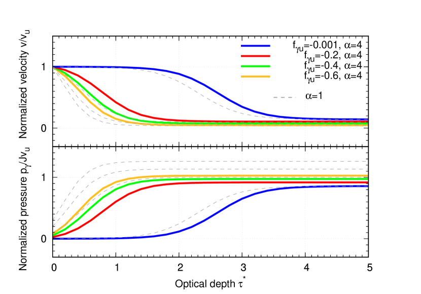
Figure 1: Normalized velocity (upper panel) and pressure (lower panel) profiles plotted as functions of the optical depth $\tau^{\star}$ for different values of the radiation energy flux upstream, $\tilde{f}_{u}=-0.001,-0.2,-0.4,-0.6$, and $\alpha=4$ (complete beaming for $c/v_{u}=4$) and $\alpha=1$, where $\tilde{f}_{\gamma u}=-2\alpha\tilde{p}_{\gamma u}$. The blue line corresponds to an almost infinite shock.

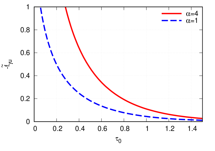
Figure 2: A plot of $|{\tilde{f}}_{\gamma u}|$ versus $\tau_{0}$ for $\alpha=1$ (dashed line) and $\alpha=4$ (solid line).

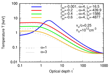
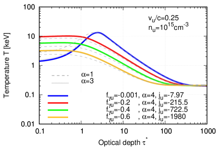
Figure 3: Temperature profiles as functions of the optical depth $\tau^{\star}$ for the upstream velocity $v_{u}/c=0.25$ and densities $n_{u}=10^{12}$ cm^-3 (left-hand panel) and $n_{u}=10^{15}$ cm^-3 (right-hand panel). We take the radiation energy flux upstream $\tilde{f}_{u}=-0.001,-0.2,-0.4,-0.6$, and $\alpha=4$ (complete beaming for $c/v_{u}=4$; solid lines), $\alpha=3$ (isotropic case; dotted lines), and $\alpha=1$ (dashed lines) where $\tilde{f}_{\gamma u}=-2\alpha\tilde{p}_{\gamma u}$. The photon number flux upstream is adjusted to satisfy the boundary condition $j_{\gamma u}=f_{\gamma u}/3kT_{u}$.

2.3 Computing the temperature profile

The local temperature can be obtained from the relation

$$kT(x)=\frac{p_{\gamma}(x)}{n_{\gamma}(x)},$$ (13)

once the photon density is known. The evolution of the latter is governed by the equation

$$\frac{dj_{\gamma}}{dx}=\dot{n}_{\gamma},$$ (14)

with $j_{\gamma}$ given by Eq. (1), where $\dot{n}_{\gamma}$ is a photon source that accounts for all emission and absorption processes. Under the conditions envisaged here, photon generation is dominated by bremsstrahlung emission of the hot electrons. Absorption can be accounted for by including the suppression factor

$$f_{ab}=1-\frac{n_{\gamma}}{n_{BB}}=1-2.4\times 10^{-31}\Theta^{-3}n_{\gamma},$$ (15)

where $\Theta=kT/m_{e}c^{2}$ (Weaver, 1976) that considerably simplifies the calculations and is sufficient for our purposes. Specifically, $\dot{n}_{\gamma}=Q_{ff}f_{ab}$. For the thermal bremsstrahlung source, we adopt the form (Eq. (3.2) in Weaver (1976)):

$$Q_{ff}=\frac{1}{2}\alpha_{e}n_{p}n_{e}\sigma_{T}c\Theta^{-1/2}\Lambda_{eff},$$ (16)

expressed in terms of the fine structure constant $\alpha_{e}$ and the coefficient $\Lambda_{eff}=E_{1}(y)g_{eff}(y)$, where $y\equiv h\nu_{c}/kT$, $E_{1}(y)$ is the first-order exponential integral function, which satisfies $E_{1}(y)\simeq-\ln y-0.5772$ at $y\ll 1$, and $g_{eff}\approx 1.226-0.475\ln y+0.0013(\ln y)^{2}$ is the Gaunt factor. The cut-off frequency, $\nu_{c}(T,n)$, corresponds to the energy below which newly generated soft photons are re-absorbed before being boosted to the thermal peak by inverse Compton scattering. It is derived in Katz et al. (2010) and is given explicitly by their equation (11), $y=({kT}/{m_{e}c^{2}})^{-9/4}({\alpha_{e}g_{ff}(m_{e}c^{2})^{-3}h^{3}c^{3}n}/{32\pi})^{1/2}$. Combining equations (1), (14), and (16), we finally arrive at

$$\frac{d}{d\tau^{\star}}\left[\tilde{n}_{\gamma}\tilde{v}-\frac{1}{3}\frac{d\tilde{n}_{\gamma}}{d\tau^{\star}}\right]=\frac{\alpha_{e}}{2}\tilde{n}(c/v_{u})^{2}\Theta^{-1/2}\Lambda_{eff}f_{ab}\equiv 3\tilde{v}\tilde{Q}_{\gamma},$$ (17)

with $\tilde{n}_{\gamma}\equiv n_{\gamma}/n_{u}=(m_{p}/m_{e})(v_{u}/c)^{2}(\tilde{p}_{\gamma}/\Theta)$ for a given solution $\tilde{p}_{\gamma}(\tau^{\star})$ of the shock equations, specifically Eqs. (6) and (9). Note that the photon flux is normalized as ${\tilde{j}}_{\gamma}\equiv j_{\gamma}/n_{u}v_{u}=\tilde{n}_{\gamma}\tilde{v}-(1/3){d\tilde{n}_{\gamma}}/{d\tau^{\star}}$.

This equation is subject to the boundary conditions $dj_{\gamma}/d\tau^{\star}\rightarrow 0$ at $\tau^{\star}\rightarrow\infty$, and

$$j_{\gamma u}=\frac{f_{\gamma u}}{3kT_{u}}$$ (18)

at $\tau^{\star}=0$, where $T_{u}$ is the value of the temperature there. The solution that satisfies the boundary conditions is obtained with the Green’s function method as

$${\tilde{n}_{\gamma}}({\tilde{x}})=\frac{{\tilde{j}_{\gamma u}}}{{\tilde{v}_{\rm eff}}({\tilde{x}})}+\int_{0}^{\infty}G({\tilde{x}},{\tilde{y}}){\tilde{Q}_{\gamma}}({\tilde{y}})d{\tilde{y}},$$ (19)

where we introduce a new coordinate,

$$d{\tilde{x}}=3(v_{u}/c)n_{u}\sigma_{T}dx=3\tilde{v}d\tau^{\star},$$ (20)

and the Green’s function is

$$G({\tilde{x}},{\tilde{y}})=\left\{\begin{array}[]{ll}\frac{\displaystyle e^{{\tilde{x}}-{\tilde{y}}}}{\displaystyle{\tilde{v}_{\rm eff}}(\tilde{y})},&({\tilde{x}}\leq{\tilde{y}})\\ \frac{\displaystyle 1}{\displaystyle{\tilde{v}_{\rm eff}}({\tilde{x}})},&({\tilde{x}}>{\tilde{y}})\end{array}\right.$$ (23)

with an effective velocity

$$\frac{1}{{\tilde{v}_{\rm eff}}({\tilde{x}})}=\int_{\tilde{x}}^{\infty}\frac{e^{-({\tilde{x}}^{\prime}-{\tilde{x}})}}{{\tilde{v}}({\tilde{x}}^{\prime})}d{\tilde{x}}^{\prime}.$$ (24)

The boundary condition $dj_{\gamma}/d\tau^{\star}\to 0$ at the far downstream, $\tau^{\star}\to\infty$, is satisfied thanks to the suppression factor $f_{ab}$ in Eq. (15), that leads to a thermodynamic equilibrium, $\tilde{Q}_{\gamma}\to 0$. A numerical solution of Eq. (19) is obtained through iteration: $\tilde{Q}_{\gamma}$ is calculated from $\Theta$ (and $\tilde{n}_{\gamma}$ in $f_{ab}$) with Eq. (17), $\tilde{n}_{\gamma}$ is calculated from $\tilde{Q}_{\gamma}$ with Eq. (19), and $\Theta$ is calculated from $\tilde{n}_{\gamma}$ with Eq. (13). The convergence of the iteration becomes slow for large $|\tilde{f}_{\gamma u}|$. The photon flux upstream, ${\tilde{j}}_{\gamma u}$, is adjusted to satisfy the boundary condition in Eq. (18) by the second numerical iteration.

Figure 3 shows the temperature profiles thereby computed for an upstream velocity $v_{u}/c=0.25$, two values of the density, $n_{u}=10^{12}$ cm^-3 (left-hand panel) and $n_{u}=10^{15}$ cm^-3 (right-hand panel), and different values of the escape parameter, $\tilde{f}_{u}=-0.001,-0.2,-0.4$, and $-0.6$, as indicated. The thick solid lines are solutions obtained for $\alpha=4$ in Eq. (12) (complete beaming), the thin dotted lines for $\alpha=3$ (isotropic case), and the dashed lines for $\alpha=1$. The case $\tilde{f}_{u}=-0.001$, that corresponds to a nearly infinite shock, is consistent with the previous calculations outlined in Weaver (1976) and Katz et al. (2010) for $\alpha=4$ and $3$. For $\alpha=1$, the drop-off at small optical depths somewhat deviates from the infinite shock solution. This is due to the higher upstream pressure required to obtain the same losses. We verified that it does converge to the infinite shock case for smaller values of $\tilde{f}_{\gamma u}$.

Figure 4 shows the photon number fluxes $|{\tilde{j}}_{\gamma}|$ as functions of the optical depth $\tau^{\star}$ for the upstream velocity $v_{u}/c=0.25$ and density $n_{u}=10^{12}$ cm^-3 and different escape fractions $\tilde{f}_{u}=-0.001,-0.2,-0.4$, and $-0.6$ with $\alpha=4$. The negative flux part is plotted by dashed lines. As photons escape, the photon number fluxes change the sign at $\tau^{\star}\gtrsim 2$, i.e., after the shock compression as we can see from Fig. 1. This is consistent with the picture that the photons generated by the shock compression diffuse upstream to be released as breakout emission. Furthermore, we can check that the sign changes at $\sim 1/4$ of the diffusion length $\Delta x\sim c/vn\sigma_{T}$.

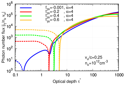
Figure 4: Photon number fluxes $|{\tilde{j}}_{\gamma}|$ as functions of the optical depth $\tau^{\star}$ for the upstream velocity $v_{u}/c=0.25$ and density $n_{u}=10^{12}$ cm^-3. The negative fluxes are shown by dashed lines. We take the radiation energy flux upstream $\tilde{f}_{u}=-0.001,-0.2,-0.4$, and $-0.6$, and $\alpha=4$ (complete beaming for $c/v_{u}=4$).

As Fig. 3 indicates, the temperature of the escaping radiation decreases as the escaping flux $|{\tilde{f}}_{\gamma u}|$ increases. This is seen more clearly in Fig 5, where the upstream temperature is plotted against $|{\tilde{f}}_{\gamma u}|$. The temperature declines exponentially as the loss rate increases. Consequently, a spectral softening is anticipated during the course of the breakout. The sole reason for this behavior is the increase in the shock compression ratio with increasing losses, that leads to enhancement of the photon generation rate. To get some insight, we give a simple heuristic derivation of the upstream temperature: the escaping photons is generated within $\sim 1/4$ of diffusion length $\Delta x\sim c/vn\sigma_{T}$ so as not to be swept downstream (see Fig. 4). From Eqs. (14) and (16), the photon number flux near the upstream boundary is approximately given by

$$j_{\gamma}\sim Q_{ff}f_{ab}\Delta x/4\sim\alpha_{e}nc^{2}\Theta^{-1/2}\Lambda_{eff}/8v,$$ (25)

where we can put $f_{ab}\approx 1$. Here, the photons are mainly generated after the deceleration down to $v\sim v_{d}$ (or the compression $n\propto 1/v$). The number flux also satisfies the boundary condition in Eq. (18). By approximating $j_{\gamma}\sim|j_{\gamma u}|$ and $T\sim T_{u}$, we obtain an analytic approximation for the upstream temperature as

$$kT_{u}\sim\frac{1}{m_{e}c^{2}}\left(\frac{4m_{p}v_{u}^{2}v_{d}^{2}{\tilde{f}}_{\gamma u}}{3\alpha_{e}c^{2}\Lambda_{eff}}\right)^{2}.$$ (26)

This relation is shown in Fig. 5 by dashed lines, and elucidates the dependence of $T_{u}$ on $v_{d}$,

To examine the dependence on the shock velocity, we obtained solutions for $v_{u}/c=0.08$ (see Fig. 6). Contrary to the previous case, the temperature profile is essentially independent of the loss rate. This is expected since at such low velocity, the characteristic length over which a full thermodynamic equilibrium is established becomes comparable to the shock width. The numerical result exhibited in Fig. 6 is in a good agreement with the analytic result derived in equation (14) in Katz et al. (2010).

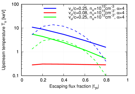
Figure 5: Expected temperature evolution as a function of the radiation energy flux upstream (i.e., escaping flux fraction) $|\tilde{f}_{u}|$. The temperature peaks just after the breakout and exponentially decreases for fast shocks with $v_{u}/c\lower 2.15277pt\hbox{$\;\buildrel>\over{\sim}\;$}0.1$. We also plot the analytic approximation for the upstream temperature in Eq. (26) by dashed lines with using $\Lambda_{eff}=20$ for $v_{u}/c=0.25$ and $n_{u}=10^{15}$ cm^-3, and $\Lambda_{eff}=40$ for $v_{u}/c=0.25$ and $n_{u}=10^{12}$ cm^-3.

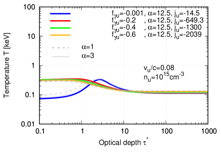
Figure 6: Same as the right-hand panel in Fig. 3, but for $v_{u}/c=0.08$.

2.4 Caveats

The quasi-steady, planar approximation invoked in our analysis is questionable, since at breakout the diffusion time across the shock and the expansion time are comparable. On the one hand, dynamical effects might lead to some suppression of the photon production rate inside the shock and a corresponding increase of the immediate downstream temperature. On the other hand, sphericity might give rise to adiabatic losses of the expanding shocked layer. What is the net effect on the observed temperature is difficult to assess.

Another concern is the validity of the RMS solution. Within the diffusion approximation it has been found above that the radiation can support the shock even when the losses become large. This requires causal contact across the shock to allow its adjustment of the changing conditions. In reality a subshock will eventually form due to dynamical effects, which may alter the spectrum. Note, however, that the jump conditions across the entire shock transition are determined by the overall energy and momentum fluxes upstream (i.e., incoming flux minus escaping flux). Consequently, the presence of a subshock will not affect the downstream temperature considerably. It can lead to particle acceleration that might give rise to formation of a non-thermal tail via comptonization once the subshock energy becomes substantial, but is unlikely to alter significantly the evolution of the downstream temperature during breakout. A complete treatment of these effects is beyond the scope of this paper (see also Sec. 3.2).

3 Observational consequences

As the shock emerges from the stellar envelope, it starts propagating in the wind until breaking out at some radius $R_{bo}$ at time $t_{bo}=R_{bo}/v_{bo}$ at velocity $v_{bo}$. In the following, we adopt a wind profile of the form $\rho_{w}=A(r/R_{\star})^{-2}$, here $R_{\star}$ denotes the progenitor’s radius. The shock accelerates during propagating through the decreasing density profile of the stellar envelope, and the profile of the accelerated ejecta can be expressed in terms of the maximum velocity $v_{0}$ of the ejecta subsequent to the shock emergence from the stellar envelope in the form (Nakar & Sari, 2010)

$$E(v)=E_{0}(v/v_{0})^{-\lambda}=\frac{4\pi cv_{0}}{\kappa}R_{\star}^{2}(v/v_{0})^{-\lambda},$$ (27)

where $\lambda=(1+0.62n)/0.19n$, and $1.5\leq n\leq 3$ is the polytropic index that depends on the progenitor type. Here, $E_{0}$ is the total energy contained in a shell of optical depth $c/v_{0}$ with opacity $\kappa$. The breakout velocity can be readily found by equating the swept up energy, $m_{bo}v_{bo}^{2}$, where $m_{bo}=4\pi AR^{2}_{\star}R_{bo}$ is the swept-up mass, with the energy injected into the shock, $E(v_{bo})$, noting that at the breakout radius, $R_{bo}$, the optical depth of the wind, $\tau_{w,bo}=\kappa m_{bo}/4\pi R_{bo}^{2}$, satisfies $\tau_{w,bo}=c/v_{bo}$. This finally yields

$$v_{bo}=v_{0}(R_{\star}/R_{bo})^{2/(\lambda+1)}=v_{0}(R_{\star}/v_{0}t_{bo})^{2/(\lambda+3)}.$$ (28)

By employing Eqs. (A2), (A4), and (A7) for $v_{0}$ in Nakar & Sari (2010), the breakout velocity can be expressed in terms of the explosion energy, $E=10^{51}E_{51}$ erg, and ejecta mass, $M_{ej}=10~{}M_{10}~{}M_{\odot}$, as

$$v_{bo}\simeq 0.1c~{}E_{51}^{0.44}M_{10}^{-0.31}t_{bo,2}^{-0.25},$$ (29)

where $t_{bo,2}=t_{bo}/10^{2}$ s (Svirski & Nakar, 2014a, b). The above analysis predicts hard X-ray emission with a significant softening during the breakout phase for fast shocks, $v_{bo}\lower 2.15277pt\hbox{$\;\buildrel>\over{\sim}\;$}0.1c$, or, using Eq. (29), for breakouts that satisfy $t_{bo,2}\lower 2.15277pt\hbox{$\;\buildrel<\over{\sim}\;$}E_{51}^{1.76}M_{10}^{-1.24}$.

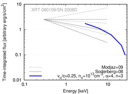
Figure 7: Time-integrated spectral energy distribution for $v_{u}/c=0.25,n_{u}=10^{13}$ cm^-3, $\alpha=4$, and $n=3$ taking the temperature softening in Fig. 5 into account. The origin of the vertical axis is arbitrary. We also plot the photon spectral indexes of a possible breakout event XRT 080109/SN 2008D, $\Gamma=2.1^{+0.3}_{-0.4}$ (Modjaz et al., 2009) and $\Gamma=2.3^{+0.3}_{-0.3}$ (Soderberg et al., 2008).

For illustration, we present in Fig. 7 the spectral energy distribution, $\nu F_{\nu}$, integrated over the duration of the breakout phase, assuming that at any given time the radiation has a thermal spectrum characterized by the local temperature at the emitting surface (i.e., the upstream temperature in our solution). To be precise, the time-integrated spectrum is given formally by

$$\int\nu F_{\nu}dt\propto\int E(\tau)|f_{\gamma u}(\tau)|\nu^{4}\left(e^{h\nu/kT(\tau)}-1\right)^{-1}~{}d\tau,$$ (30)

where $\tau\propto r^{-1}\propto v^{\lambda+2}$ is the optical depth at radius $r$ and time $t=r/v$ because the swept-up wind energy $4\pi Arv^{2}$ is equal to $E(v)\propto v^{-\lambda}$, $E(\tau)\propto v^{-\lambda}\propto\tau^{-\lambda/(\lambda+2)}$ is the shock energy at $\tau$, $f_{\gamma u}(\tau)$ is the corresponding escape parameter (see Fig. 2) by equating $\tau$ to $\tau_{0}({\tilde{f}}_{\gamma u})$ in Eqs. (11) and (12), and $T(\tau)$ is the temperature (see Fig. 5). In Fig. 7, we connect the thermal peaks for corresponding frequencies. The time-integrated spectrum spreads over a broad frequency range because of a softening during the breakout phase.

3.1 Deriving the physical parameters from the observables

The breakout pulse features three general observables – luminosity, duration, and the typical photon frequency, which we henceforth associate with the characteristic breakout temperature. Following the breakout emission, the luminosity declines, sometimes slowly, as a power law during the transition of the shock from being radiation dominated to collisionless (see discussion below), and thus the breakout observables should be associated only with the rising part of the observed signal, specifically, the luminosity is roughly the peak luminosity, the duration is the emission rise time and the temperature is roughly one-third the peak energy of the time-integrated spectrum of the rising flux. These three observables are determined by two physical parameters – the breakout velocity and radius. Thus, the model is overconstrained, whereby any two observables are sufficient to determine the physical parameters, and the third one can be used as a consistency check of the model. The luminosity and duration are related to the physical parameters through (e.g., Svirski & Nakar, 2014b):

$$t_{bo} \approx \frac{R_{bo}}{v_{bo}},$$ (31)

$$L_{bo} \approx 1.5\times 10^{42}t_{bo,2}v_{bo,-1}^{3}{\rm~{}erg~{}s}^{-1}.$$ (32)

The dependence of the radiation temperature on the velocity and radius cannot be expressed as a simple analytic formula (see equation (26) and Fig. 5). Moreover, as we have seen above it varies with time (as the escape fraction increases). However, a rough estimate of the typical breakout temperature can be obtained by finding the radiation temperature when the escape fraction is $0.5$. Figure 8 shows the typical temperature for $\tilde{f}_{u}=-0.5$ and $\alpha=4$ as a function of breakout time, for several shock velocities, $v_{u}/c=0.1,0.2,0.3$ and $0.4$. The density is determined by the opacity condition $n\sigma_{T}R_{bo}=c/v_{bo}$. With this Fig. 8, one can infer the shock velocity from the observed quantities $T_{bo}$ and $t_{bo}$. It can then be compared to the velocity obtained from $L_{bo}$, thereby testing if a given observed flare may have been the result of a shock breakout from a wind.

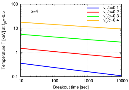
Figure 8: Typical temperature at the escape fraction $\tilde{f}_{u}=-0.5$ with $\alpha=4$ as a function of breakout time-scale for several shock velocities $v_{u}/c=0.1,0.2,0.3$, and $0.4$.

3.2 The observed light curve and spectral evolution

The above analysis relates the escaping fraction (i.e., luminosity) and the radiation temperature to the instantaneous lab time at which the quasi-steady, planar solution is obtained. It is naively anticipated that this can be directly translated into the observed light curve and time-resolved spectra during the breakout phase. However, in practice geometrical (non-planar) effects, not accounted for by our model, may alter these observables (though not the time-integrated spectrum) in ways we now describe. The main point is that since the breakout takes place once $\tau\approx c/v>1$, the photons can still interact with upstream gas also after escaping the shock. These interactions conceivably include absorption and/or scattering of photons along their path to the observer. First, let us consider absorption. Svirski et al. (2012) have shown that when the post-shock plasma is out of thermodynamic equilibrium then free-free absorption of photons that escape the shock is negligible. However, if there are partially ionized metals in the cold upstream then their X-ray opacity can be considerable. To estimate the ionization fraction, we use the ionization parameter $\xi=L/nr^{2}$, where $L$ is the luminosity of ionizing radiation and $n$ is the gas density, all expressed in cgs units. Chevalier & Irwin (2012) (and references therein) have shown that when $\xi>10^{4}$, radiation at a temperature of $\sim 10$ keV fully ionize all metals including iron. In case of a shock breakout from a stellar wind with $n\propto r^{-2}$, the ionization depends only on the shock velocity, roughly as $\xi\approx 10^{8}(v_{s}/c)^{3}$. Consequently, for the shocks considered here ($v_{s}/c\lower 2.15277pt\hbox{$\;\buildrel>\over{\sim}\;$}0.1$) we have $\xi>10^{5}$, hence photo-absorption by partially ionized metals is not expected. Next, let us consider the effect of scattering. For the shocks we consider here the Thomson optical depth encountered by a photon escaping the shock is $\sim 2$–$3$. Thus, a non-negligible fraction of the escaping photons are scattered at least once on their way to the observer by electrons at radii larger than $R_{bo}$. This scattering cannot change the emitted spectrum but it will affect the photon arrival time. Consequently, our simplified model cannot fully account for the exact shape of the X-ray light curve nor for the spectral evolution during the rising of the emission. Nevertheless, we expect that the emission will show a hard-to-soft evolution during the rise of the flux, and the time-integrated spectrum to be non-thermal, similar to the one shown in Fig. 7. Note that the spectrum is formed in a different way from the case of a breakout from a stellar surface, in which the time-integrated spectrum is the sum of radiation emitted form different positions of the shocked material.

It is worth noting that the breakout emission dominates the rise of the signal and, perhaps, the initial decay following the peak luminosity (over a duration that does not exceed the risetime), but not the entire luminosity evolution. The reason is that following the breakout of the RMS a collisionless shock is formed which is very efficient in converting the shock energy to X-rays (Svirski & Nakar, 2014a), at least as long as $\tau>1$. As a result, the observed flux following the breakout phase should exhibit a slow power-law decay until the collisionless shock reaches the full extent of the wind (Svirski et al., 2012). The transition from RMS to a fully collisionless shock is anticipated to be gradual, since the escaping radiation accelerates the plasma ahead of the shock, at radii $r>R_{bo}$, roughly to a velocity $v\approx v_{bo}(R_{bo}/r)^{2}$, and once the shocked gas that trails the radiation, and propagates at a velocity $v_{bo}$ arrives, it drives a collisionless subshock that moves at a relative velocity $v_{bo}-v$ into these pre-accelerated fluid. This subshock strengthens gradually with time until either a full conversion is established or until the shock reaches the edge of the wind. The post-shock electron temperature is set by the balance between the heating and (mainly inverse Compton) cooling and it is about $\sim 60$ keV and less (Katz et al., 2011; Murase et al., 2011; Svirski et al., 2012; Svirski & Nakar, 2014a). We leave the calculation of the spectrum during this phase to a future work.

The only event in which a fast ($>0.1c$) sub-relativistic shock breakout from a thick wind was most likely observed is the X-ray transient XRT 080109 (Soderberg et al., 2008; Mazzali et al., 2008; Modjaz et al., 2009). XRT 080109 is associated with the Type Ibc supernova 2008D, favoring a WR progenitor, which are known to eject winds (Tanaka et al., 2009; Gal-Yam et al., 2014). The X-ray peak luminosity is $3.8^{+1}_{-1}\times 10^{43}$ erg s^-1, the rise time is $\sim 50$–$100$ s and after the peak it decays roughly as $t^{-1}$ for about 300 s (Soderberg et al., 2008; Modjaz et al., 2009). The general properties of the signal are in agreement with the interpretation of a fast shock breakout from a thick wind (Chevalier & Fransson, 2008; Svirski & Nakar, 2014a, b). In this interpretation, the shock breakout emission dominates during the rise and at later times, it is possible that there is also contribution from the collisionless shock that forms following the breakout. The radio observations identify synchrotron emission and the inferred shock radius $\sim 3\times 10^{15}$ cm at $\sim 5$ d implies a shock velocity of $\sim 0.25$ c (Soderberg et al., 2008). A simple estimate, $v_{bo}t_{bo}$, implies a breakout radius $R_{bo}\sim 6\times 10^{11}$ cm and hence a density $n\sim c/v_{bo}\sigma_{T}R_{bo}\sim 10^{13}$ cm^-3. The observed spectrum is consistent with a power-law spectrum with a photon spectral index $\Gamma=2.1^{+0.3}_{-0.4}$ for the period 0–520 s (Modjaz et al., 2009) and $\Gamma=2.3^{+0.3}_{-0.3}$ (Soderberg et al., 2008), showing a significant hard-to-soft evolution (Soderberg et al., 2008). In Fig. 7, we compare the breakout spectrum computed from the model with the time-integrated spectral index of XRT 080109, which includes also emission after the peak and is therefore most likely not purely the shock breakout spectrum. It shows that the observations are broadly consistent with the model prediction. We can also apply the test presented in section 3.1 to XRT 080109. Plugging $L_{bo}=4\times 10^{43}$ erg s^-1 and $t_{bo}=100$ s into equation (32) implies $v_{bo}/c\approx 0.3$. Now, using Figure 8, we obtain $T_{bo}\approx 5$ keV for $v_{bo}/c=0.3$ and $t_{bo}=100$ s, in agreement with the observed spectrum.

We should mention that a power-law spectrum could be also produced by other mechanisms. First, bulk Compton scattering could shape a power-law spectrum because a typical photon experiences $(c/v)^{2}$ scatterings, each one giving a fractional energy increase $\sim(v/c)^{2}$ and a total average increase of order unity (Blandford & Payne, 1981a, b; Wang et al., 2007; Suzuki & Shigeyama, 2010), although the efficiency of the non-thermal emission may not be enough (Suzuki & Shigeyama, 2010). Second, as above mentioned, the collisionless shock that forms following the breakout, accelerate electrons to a temperature $\lower 2.15277pt\hbox{$\;\buildrel>\over{\sim}\;$}60$ keV. These electrons upscatter soft photons to a power-law spectrum (Svirski & Nakar, 2014a, b). Future observations of shock breakouts that will separate between the spectrum during the rise and following the peak will enable us to distinguish between emissions that comes from the breakout of the RMS and emission that interacts with electrons accelerated in the collisionless shock that follows.

4 Conclusions

We have shown that the breakout of a sub-relativistic, fast ($>0.1c$) shock from a thick stellar wind should lead to a broad time-integrated spectrum during the rise of the observed flux and, conceivably, softening of the time resolved spectrum, as shown in Figs. 5 and 7. The physical reason is that the photon generation (which decreases the temperature) is enhanced by the shock steepening during the photon escape. We applied our results to XRT 080109/SN 2008D and found them to be consistent with the observed time-integrated, and the reported softening, of the X-ray spectrum in this source in Fig. 7. We also derive a closure relation between the breakout duration, peak luminosity, and characteristic temperature in Eqs. (31) and (32) and Fig. 8, which is also found to be consistent with the observations of XRT 080109. Our calculations are based on a semi-analytic model of a planar, RMS that incorporates photon escape through the upstream plasma, treats radiative transfer in the diffusion limit, and assumes a quasi-steady evolution during the breakout phase.

While the time-integrated spectrum of the breakout signal is a robust feature, the X-ray light curve and the time-resolved spectral evolution may be altered by the interaction of the escaping radiation with the plasma ahead of the RMS, at radii larger than the breakout radius, where the planar approximation invoked in our analysis breaks down. In particular, acceleration of the unshocked fluid ahead of the RMS by the escaping radiation is expected to lead to the gradual emergence of a collisionless sub-shock that strengthens over a time comparable to or even longer than the breakout time. This intermediate transition from the RMS phase to a fully collisionless shock might have interesting observational diagnostics yet to be explored.

References

- Abbott et al. (2017a) Abbott B., et al., 2017a, Phys. Rev. Lett., 119, 161101
- Abbott et al. (2017b) Abbott B. P., et al., 2017b, Astrophys. J., 848, L12
- Balberg & Loeb (2011) Balberg S., Loeb A., 2011, MNRAS, 414, 1715
- Blandford & Payne (1981a) Blandford R. D., Payne D. G., 1981a, MNRAS, 194, 1033
- Blandford & Payne (1981b) Blandford R. D., Payne D. G., 1981b, MNRAS, 194, 1041
- Campana et al. (2006) Campana S., et al., 2006, Nature, 442, 1008
- Chevalier & Fransson (2008) Chevalier R. A., Fransson C., 2008, ApJ, 683, L135
- Chevalier & Irwin (2012) Chevalier R. A., Irwin C. M., 2012, ApJ, 747, L17
- Forster et al. (2018) Forster F., et al., 2018, Nature Astronomy, 2, 808
- Gal-Yam et al. (2014) Gal-Yam A., et al., 2014, Nature, 509, 471
- Gottlieb et al. (2018) Gottlieb O., Nakar E., Piran T., Hotokezaka K., 2018, MNRAS, 479, 588
- Granot et al. (2018) Granot A., Nakar E., Levinson A., 2018, MNRAS, 476, 5453
- Ioka & Nakamura (2018) Ioka K., Nakamura T., 2018, Progress of Theoretical and Experimental Physics, 2018, 043E02
- Ito et al. (2018) Ito H., Levinson A., Stern B. E., Nagataki S., 2018, MNRAS, 474, 2828
- Kasliwal et al. (2017) Kasliwal M. M., et al., 2017, Science, 358, 1559
- Katz et al. (2010) Katz B., Budnik R., Waxman E., 2010, ApJ, 716, 781
- Katz et al. (2011) Katz B., Sapir N., Waxman E., 2011, preprint, p. arXiv:1106.1898 (arXiv:1106.1898)
- Katz et al. (2012) Katz B., Sapir N., Waxman E., 2012, ApJ, 747, 147
- Kyutoku et al. (2014) Kyutoku K., Ioka K., Shibata M., 2014, MNRAS, 437, L6
- Mazzali et al. (2008) Mazzali P. A., et al., 2008, Science, 321, 1185
- Modjaz et al. (2009) Modjaz M., et al., 2009, ApJ, 702, 226
- Moriya et al. (2011) Moriya T., Tominaga N., Blinnikov S. I., Baklanov P. V., Sorokina E. I., 2011, MNRAS, 415, 199
- Murase et al. (2011) Murase K., Thompson T. A., Lacki B. C., Beacom J. F., 2011, Phys. Rev. D, 84, 043003
- Nakar & Sari (2010) Nakar E., Sari R., 2010, ApJ, 725, 904
- Nakar & Sari (2012) Nakar E., Sari R., 2012, ApJ, 747, 88
- Nakar et al. (2018) Nakar E., Gottlieb O., Piran T., Kasliwal M. M., Hallinan G., 2018, ApJ, 867, 18
- Ofek et al. (2014) Ofek E. O., et al., 2014, ApJ, 789, 104
- Sapir et al. (2011) Sapir N., Katz B., Waxman E., 2011, ApJ, 742, 36
- Sapir et al. (2013) Sapir N., Katz B., Waxman E., 2013, ApJ, 774, 79
- Soderberg et al. (2008) Soderberg A. M., et al., 2008, Nature, 453, 469
- Suzuki & Shigeyama (2010) Suzuki A., Shigeyama T., 2010, ApJ, 719, 881
- Svirski & Nakar (2014a) Svirski G., Nakar E., 2014a, ApJ, 788, 113
- Svirski & Nakar (2014b) Svirski G., Nakar E., 2014b, ApJ, 788, L14
- Svirski et al. (2012) Svirski G., Nakar E., Sari R., 2012, ApJ, 759, 108
- Tan et al. (2001) Tan J. C., Matzner C. D., McKee C. F., 2001, ApJ, 551, 946
- Tanaka et al. (2009) Tanaka M., et al., 2009, ApJ, 692, 1131
- Wang et al. (2007) Wang X.-Y., Li Z., Waxman E., Mészáros P., 2007, ApJ, 664, 1026
- Waxman & Katz (2017) Waxman E., Katz B., 2017, Shock Breakout Theory. p. 967, doi:10.1007/978-3-319-21846-5_33
- Waxman et al. (2007) Waxman E., Mészáros P., Campana S., 2007, ApJ, 667, 351
- Weaver (1976) Weaver T. A., 1976, ApJS, 32, 233
- Yaron et al. (2017) Yaron O., et al., 2017, Nature Physics, 13, 510