Sesquickselect: One and a half pivots for cache-efficient selection

Abstract

Abstract:   Because of unmatched improvements in CPU performance, memory transfers have become a bottleneck of program execution. As discovered in recent years, this also affects sorting in internal memory. Since partitioning around several pivots reduces overall memory transfers, we have seen renewed interest in multiway Quicksort. Here, we analyze in how far multiway partitioning helps in Quickselect.

We compute the expected number of comparisons and scanned elements (approximating memory transfers) for a generic class of (non-adaptive) multiway Quickselect and show that three or more pivots are not helpful, but two pivots are. Moreover, we consider “adaptive” variants which choose partitioning and pivot-selection methods in each recursive step from a finite set of alternatives depending on the current (relative) sought rank. We show that “Sesquickselect”, a new Quickselect variant that uses either one or two pivots, makes better use of small samples w. r. t. memory transfers than other Quickselect variants.

1 Introduction

We consider the selection problem: finding the $m$th smallest element within an unsorted array of $n$ distinct elements. Quickselect [17] is the earliest (published) algorithm for general selection that runs in linear time (in expectation), and it forms the basis of practical implementations and more advanced algorithms. From a theoretical perspective, this problem might be considered solved: The Floyd-Rivest algorithm [12, 22] uses $n+\min\{m,n-m\}+o(n)$ comparisons in expectation, and this is optimal up to lower order terms [8]. The Floyd-Rivest algorithm is a variant of Quickselect that uses a large random sample of $\Theta(n^{2/3}\log^{1/3}n)$ elements from which it (recursively) selects two pivots $P_{1}$ and $P_{2}$, $P_{1}<P_{2}$, so that their ranks surround $m$ with high probability. Partitioning the input into the elements $<P_{1}$, between $P_{1}$ and $P_{2}$, and $>P_{2}$, respectively, yields a subproblem of size $o(n)$ with high probability.

Standard libraries do not use the asymptotically optimal algorithms [38, 1], presumably because for moderate-size inputs, lower order terms and their large hidden constants are not negligible, making variants with less overhead desirable. For example, the GNU implementation of the C++ STL uses introspective median-of-3 Quickselect for std:​:nth_element. Introspective sorting was suggested by Musser [31] and refined by Valois [38].

Given the similarity of Quicksort and Quickselect, it is natural and tempting to employ the same optimizations for selection that work well for sorting. Indeed, this is exactly what is done in the GNU STL; the Quickselect implementation uses the same partitioning method, the same pivot rule (median of three elements), the same protection mechanism against bad-case inputs (a recursion-depth limit of $2\lceil\lg(n+1)\rceil$ with a $\Theta(n\log n)$ worst-case method based on heapsort), and the same base case for the recursion (Insertionsort) as in the Quicksort implementation. On second thought, some of these design decisions are quite questionable in the context of selection. First, a linear worst case can be achieved instead of the $\Theta(n\log n)$ one [6, 38]. Second, it is known that choosing the pivot adaptively, i. e., depending on the value of $m$ (mimicking the asymptotically optimal Floyd-Rivest algorithm!) improves the average costs by a significant factor even for small sample sizes [29].

Finally, in light of the recent success of multi-pivot Quicksort [4, 27, 32, 39], a question programmers will face is whether and how multiway partitioning should also be used for Quickselect. Using YBB-partitioning – the dual-pivot method used in Arrays.sort of Oracle’s Java runtime library [43, 42] – was shown to be of no advantage for Quickselect w. r. t. the number of comparisons (averaging over all possible ranks to be selected) [41]. YBB partitioning can reduce the comparison count in sorting, but the main advantage of multiway partitioning lies in saving memory transfers, and indeed, the latter is improved using dual-pivot Quickselect (see §​ 4). The purpose of this article is thus a comprehensive assessment of the potential of multiway partitioning in Quickselect.

To this end, we present an average-case analysis of both classical cost measures and memory transfers. The latter is formalized as the number of scanned elements: the accumulated range scanned by all index/pointer variables used in the partitioning strategy. This has been shown to be a good indicator for the number of cache misses that occur during partitioning [32, 4].

Our focus is on low-overhead algorithms suitable for library implementations, and hence on small fixed-size samples. Taking inspiration from Floyd-Rivest, we propose “Sesquickselect”, an adaptive Quickselect variant that uses either one or two pivots from a sample of $k$ elements, and we give strong evidence for its optimality w. r. t. scanned elements subject to a given sample size.

Overview and Method

We first consider multiway partitioning and pivot sampling in full generality (partitioning into any constant number $s\geq 2$ of segments while choosing pivots from samples of any constant size $k$), under the assumption that a uniformly chosen random rank is searched. These so-called “grand averages” [28] can be computed using a distributional master theorem [39] derived from Roura’s continuous master theorem [34]. We can conclude that more than three segments are indeed not helpful in Quickselect. This matches the intuition that a large $s$ “should” not help since all but one segment will be discarded for good, making further subdivisions superfluous. The precise argument requires some care, though.

Unfortunately, the grand-average analysis does not extend to adaptive methods like Sesquickselect. For the second part, we hence consider selecting the $\alpha$-quantile in a large array for a fixed $\alpha\in(0,1)$ (extending techniques from [29]). We give an elementary proof for the correctness of a resulting integral equation for the leading-term coefficient as a function of $\alpha$ (under reasonable assumptions fulfilled for our applications) that appears to be novel.

The setting with two parameters makes computations appreciably more challenging. For Quickselect with YBB partitioning (without pivot sampling) and Sesquickselect with $k=2$ we solve the integral equations analytically, and we obtain precise numerical solutions for more general cases. From these, we can derive promising candidates of cache-optimal Quickselect variants for all practical sample sizes.

Outline

We give an overview of previous work in the remainder of this section. §​ 2 introduces notation and preliminaries. In §​ 3, we state a general distributional recurrence of costs. §​ 4 discusses the analysis for random ranks. We then switch to fixed ranks and derive the integral equation in §​ 5. We solve it for Quickselect with YBB-partitioning (§​ 6) and for the novel “Sesquickselect” algorithm (§​ 7). Our paper concludes with a discussion of our findings (§​ 8).

The appendix contains a comprehensive list of notation, as well as some technical proofs and details of the computations.

1.1 Previous Work

The first published analysis of (classic) Quickselect by Knuth served as one of two illustrating examples in an invited address at the IFIP Congress 1971, with the goal to advertise the emerging area of analysis of algorithms [24, 25]. The expected number of comparisons in classic Quickselect is $\mathbb{E}[C_{n,m}]\mathchoice{\mathrel{\;\;{=}\;\;}}{\mathrel{=}}{\mathrel{=}}{\mathrel{=}}2\bigl{(}(n+1)H_{n}-(n+3-m)H_{n+1-m}-(m+2)H_{m}+n+3\bigr{)},$ where $H_{n}=\sum_{i=1}^{n}\!\frac{1}{i}$.

An asymptotic approximation for selecting the $\alpha$-quantile, $\alpha\in(0,1)$ fixed, follows with $m=\alpha n$: $\mathbb{E}[C_{n,\alpha n}]\mathchoice{\mathrel{\;\;{=}\;\;}}{\mathrel{=}}{\mathrel{=}}{\mathrel{=}}2(h(\alpha)+1)\cdot n\mathchoice{\mathbin{\>{-}\>}}{\mathbin{-}}{\mathbin{-}}{\mathbin{-}}8\ln n\mathchoice{\mathbin{\;{\pm}\;}}{\mathbin{\pm}}{\mathbin{\pm}}{\mathbin{\pm}}O(1)$, $n\to\infty$, where $h(x)=-x\ln x-(1-x)\ln(1-x)$; (here we set $0\ln 0\colonequals 0$).

Quickselect has been extensively studied. The variance is quadratic and precisely known [33, 21]; large deviations from the mean are very unlikely [9, 14]. Stochastic limits laws have been established for the random costs divided by $n$ for random ranks [28], small ranks [18] and fixed quantiles [16].

Like for Quicksort, better pivot selection methods are important in Quickselect. The widely used median-of-three version was analyzed in [2] and [20], and the generalization of using the median of any fixed size sample (“median-of-$k$”) in [30] (expectation and variance for random ranks) and in [15] (for fixed ranks); refined limit laws for the case where $k$ grows polynomially with $n$ were recently derived in [37]. Choosing the order statistic of the sample depending on $m/n$ was studied in [29] (w. r. t. expectation) and [23] (limit laws, including growing $k$).

If the objects to select from are strings, symbol comparisons rather than key comparisons are the measure of interest; Quickselect has linear expected cost also in this model [7]. Quickselect with YBB partitioning was analyzed in [41] and Krenn [26] considered the comparison-optimal dual-pivot partitioning method of Aumüller and Dietzfelbinger [3].

2 Preliminaries

We introduce important notation here; see Appendix A for a comprehensive list. $O$-terms are bounds on the absolute value; we write $g=f\pm O(e)$ to emphasize this. $f\sim g$ means $f/g\to 1$. Vector’s are written in boldface, e. g., $\bm{\mathbold{x}}=(x_{1},x_{2},x_{3})$, and operations are understood componentwise: $\bm{\mathbold{x}}+1=(x_{1}+1,x_{2}+1,x_{3}+1)$. We use the notation $x^{\overline{n}}$ and $x^{\underline{n}}$ of [13] for rising resp. falling (factorial) powers. (The former is also known as Pochhammer function).

We use capital letters for random variables and $\mathbb{E}$ for expectation. $X\mathchoice{\mathrel{\overset{\raisebox{0.0pt}{$\scriptstyle\cal D$}}{=}}}{\mathrel{\mathchoice{\hbox{\makebox[10.55551pt][c]{\makebox[0.0pt][c]{$\displaystyle\overset{\raisebox{-4.30554pt}{$\scriptscriptstyle\cal D$}}{=}$}}}}{\hbox{\makebox[10.55551pt][c]{\makebox[0.0pt][c]{$\textstyle\overset{\raisebox{-4.30554pt}{$\scriptscriptstyle\cal D$}}{=}$}}}}{\hbox{\makebox[8.22217pt][c]{\makebox[0.0pt][c]{$\scriptstyle\overset{\raisebox{-3.01389pt}{$\scriptscriptstyle\cal D$}}{=}$}}}}{\hbox{\makebox[6.66661pt][c]{\makebox[0.0pt][c]{$\scriptscriptstyle\overset{\raisebox{-2.15277pt}{$\scriptscriptstyle\cal D$}}{=}$}}}}}}{\mathrel{\overset{\cal D}{=}}}{\mathrel{\overset{\cal D}{=}}}Y$ denotes equality in distribution. $\mathcal{U}[1..n]$ is the discrete uniform distribution over $[1..n]$, $\mathcal{U}(0,1)$ the continuous uniform distribution over $(0,1)$. We next recall the beta distribution and some of its properties. It will play a pivotal role in our analysis.

2.1 The beta distribution and its relatives

The beta distribution has two parameters $\alpha,\beta\in\mathbb{R}_{>0}$ and is written as $\mathrm{Beta}(\alpha,\beta)$. If $X\mathchoice{\mathrel{\overset{\raisebox{0.0pt}{$\scriptstyle\cal D$}}{=}}}{\mathrel{\mathchoice{\hbox{\makebox[10.55551pt][c]{\makebox[0.0pt][c]{$\displaystyle\overset{\raisebox{-4.30554pt}{$\scriptscriptstyle\cal D$}}{=}$}}}}{\hbox{\makebox[10.55551pt][c]{\makebox[0.0pt][c]{$\textstyle\overset{\raisebox{-4.30554pt}{$\scriptscriptstyle\cal D$}}{=}$}}}}{\hbox{\makebox[8.22217pt][c]{\makebox[0.0pt][c]{$\scriptstyle\overset{\raisebox{-3.01389pt}{$\scriptscriptstyle\cal D$}}{=}$}}}}{\hbox{\makebox[6.66661pt][c]{\makebox[0.0pt][c]{$\scriptscriptstyle\overset{\raisebox{-2.15277pt}{$\scriptscriptstyle\cal D$}}{=}$}}}}}}{\mathrel{\overset{\cal D}{=}}}{\mathrel{\overset{\cal D}{=}}}\mathrm{Beta}(\alpha,\beta)$, we have $X\in(0,1)$ and $X$ has the density

$$f(x) \mathchoice{\mathrel{\;{=}\;}}{\mathrel{=}}{\mathrel{=}}{\mathrel{=}}\frac{x^{\alpha-1}(1-x)^{\beta-1}}{\mathrm{B}(\alpha,\beta)},\qquad x\in(0,1),$$

where $\mathrm{B}(\alpha,\beta)=\Gamma(\alpha)\Gamma(\beta)/\Gamma(\alpha+\beta)$ is the beta function. The reason why the beta arise in our analysis is its connection to order statistics: If we assume the input consists of $n$ i. i. d. (independent and identically distributed) $\mathcal{U}(0,1)$ random variables, the $\ell$th smallest element of a sample of $k$ elements has a $\mathrm{Beta}(\ell,k+1-\ell)$ distribution.

For multi-pivot methods, we will encounter the Dirichlet distribution $\mathrm{Dir}(\bm{\mathbold{\alpha}})$, which is the multivariate version of the beta distribution. For $X\mathchoice{\mathrel{\overset{\raisebox{0.0pt}{$\scriptstyle\cal D$}}{=}}}{\mathrel{\mathchoice{\hbox{\makebox[10.55551pt][c]{\makebox[0.0pt][c]{$\displaystyle\overset{\raisebox{-4.30554pt}{$\scriptscriptstyle\cal D$}}{=}$}}}}{\hbox{\makebox[10.55551pt][c]{\makebox[0.0pt][c]{$\textstyle\overset{\raisebox{-4.30554pt}{$\scriptscriptstyle\cal D$}}{=}$}}}}{\hbox{\makebox[8.22217pt][c]{\makebox[0.0pt][c]{$\scriptstyle\overset{\raisebox{-3.01389pt}{$\scriptscriptstyle\cal D$}}{=}$}}}}{\hbox{\makebox[6.66661pt][c]{\makebox[0.0pt][c]{$\scriptscriptstyle\overset{\raisebox{-2.15277pt}{$\scriptscriptstyle\cal D$}}{=}$}}}}}}{\mathrel{\overset{\cal D}{=}}}{\mathrel{\overset{\cal D}{=}}}\mathrm{Dir}(\bm{\mathbold{\alpha}})$ with $\bm{\mathbold{\alpha}}\in\mathbb{R}_{>0}^{d}$, we use the convention that $X_{d}=1-X_{1}-\cdots-X_{d-1}$ and specify $\bm{\mathbold{X}}$ as a $d$-dimensional vector. Then $\bm{\mathbold{X}}$ has the density $f(\bm{\mathbold{x}})=\bm{\mathbold{x}}^{\bm{\mathbold{\alpha}}-1}/\mathrm{B}(\bm{\mathbold{\alpha}})$, where $\mathrm{B}(\bm{\mathbold{\alpha}})=\Gamma(\alpha_{1})\cdots\Gamma(\alpha_{d})/\Gamma(\alpha_{1}+\cdots\alpha_{d})$ is the $d$-dimensional beta function.

For subproblem sizes, we will furthermore find the Dirichlet-multinomial distribution $\mathrm{DirMult}(n,\bm{\mathbold{\alpha}})\mathchoice{\mathrel{\overset{\raisebox{0.0pt}{$\scriptstyle\cal D$}}{=}}}{\mathrel{\mathchoice{\hbox{\makebox[10.55551pt][c]{\makebox[0.0pt][c]{$\displaystyle\overset{\raisebox{-4.30554pt}{$\scriptscriptstyle\cal D$}}{=}$}}}}{\hbox{\makebox[10.55551pt][c]{\makebox[0.0pt][c]{$\textstyle\overset{\raisebox{-4.30554pt}{$\scriptscriptstyle\cal D$}}{=}$}}}}{\hbox{\makebox[8.22217pt][c]{\makebox[0.0pt][c]{$\scriptstyle\overset{\raisebox{-3.01389pt}{$\scriptscriptstyle\cal D$}}{=}$}}}}{\hbox{\makebox[6.66661pt][c]{\makebox[0.0pt][c]{$\scriptscriptstyle\overset{\raisebox{-2.15277pt}{$\scriptscriptstyle\cal D$}}{=}$}}}}}}{\mathrel{\overset{\cal D}{=}}}{\mathrel{\overset{\cal D}{=}}}\mathrm{Mult}(n,\mathrm{Dir}(\bm{\mathbold{\alpha}}))$, which is a mixed multinomial distribution with a Dirichlet-distributed parameter. For the 2d case, the distribution is called beta binomial distribution, written as $\mathrm{BetaBin}(n,\alpha,\beta)$.

Since the binomial distribution is sharply concentrated, one can use Chernoff bounds to show that $\mathrm{BetaBin}(n,\alpha,\beta)/n$ converges to $\mathrm{Beta}(\alpha,\beta)$ in a specific sense. We can obtain stronger error bounds by directly comparing the PDFs, and the argument generalizes to higher dimensions. The two-dimensional case appears in [39, Lemma 2.38]; here we extend it to general (fixed) $s\geq 2$. We following the notation used there, in particular we write $\Sigma\bm{\mathbold{x}}=\sum_{i=1}^{s}x_{i}$.

Lemma 2.1 (Local Limit Law for Dirichlet-multinomial):

Let $(\bm{\mathbold{I}}^{\smash{(}n\smash{)}})_{n\in\mathbb{N}_{\geq 1}}$ be a family of random variables with Dirichlet-multinomial distribution, $\bm{\mathbold{I}}^{\smash{(}n\smash{)}}\mathchoice{\mathrel{\overset{\raisebox{0.0pt}{$\scriptstyle\cal D$}}{=}}}{\mathrel{\mathchoice{\hbox{\makebox[10.55551pt][c]{\makebox[0.0pt][c]{$\displaystyle\overset{\raisebox{-4.30554pt}{$\scriptscriptstyle\cal D$}}{=}$}}}}{\hbox{\makebox[10.55551pt][c]{\makebox[0.0pt][c]{$\textstyle\overset{\raisebox{-4.30554pt}{$\scriptscriptstyle\cal D$}}{=}$}}}}{\hbox{\makebox[8.22217pt][c]{\makebox[0.0pt][c]{$\scriptstyle\overset{\raisebox{-3.01389pt}{$\scriptscriptstyle\cal D$}}{=}$}}}}{\hbox{\makebox[6.66661pt][c]{\makebox[0.0pt][c]{$\scriptscriptstyle\overset{\raisebox{-2.15277pt}{$\scriptscriptstyle\cal D$}}{=}$}}}}}}{\mathrel{\overset{\cal D}{=}}}{\mathrel{\overset{\cal D}{=}}}\mathrm{DirMult}(n,\bm{\mathbold{\alpha}})$ where $\bm{\mathbold{\alpha}}\in(\{1\}\cup\mathbb{R}_{\geq 2})^{s}$ is fixed, and let $f_{D}(\bm{\mathbold{z}})$ be the density of the $\mathrm{Dir}(\bm{\mathbold{\alpha}})$ distribution. Then we have uniformly in $\bm{\mathbold{z}}\in(0,1)^{s}$ (with $\Sigma\bm{\mathbold{z}}=1$) that

$$n^{s-1}\cdot\mathbb{P}\big{[}\bm{\mathbold{I}}^{\smash{(}n\smash{)}}=\lfloor\bm{\mathbold{z}}(n+1)\rfloor\big{]}\mathchoice{\mathrel{\;\;{=}\;\;}}{\mathrel{=}}{\mathrel{=}}{\mathrel{=}}f_{D}(\bm{\mathbold{z}})\mathchoice{\mathbin{\>{\pm}\>}}{\mathbin{\pm}}{\mathbin{\pm}}{\mathbin{\pm}}O(n^{-1}),$$

as $n\to\infty$. That is, $\bm{\mathbold{I}}^{\smash{(}n\smash{)}}/n$ converges to $\mathrm{Dir}(\bm{\mathbold{\alpha}})$ in distribution, and the probability weights converge uniformly to the limiting density at rate $O(n^{-1})$.

The proof is given in Appendix C.

Remark 2.2:

Since $f_{D}$ is a polynomial in $\bm{\mathbold{z}}$, it is in particular bounded and Lipschitz-continuous in the closed domain $\bm{\mathbold{z}}\in[0,1]^{s}$ with $\Sigma\bm{\mathbold{z}}=1$. Hence, the local limit law also holds for the random variables $\bm{\mathbold{I}}^{\smash{(}n\smash{)}}+c$ for any constant $c$. We use this for subproblem sizes, which are of this form: $J_{r}=I_{r}+t_{r}$.

2.2 Hölder-Continuity

A function $f:I\to\mathbb{R}$ defined on a bounded interval $I$ is called Hölder-continuous with exponent $h\in(0,1]$ when

$$\exists C\;\forall x,y\in I\mathchoice{\mathrel{\;{:}\;}}{\mathrel{:}}{\mathrel{:}}{\mathrel{:}}\bigl{|}f(x)-f(y)\bigr{|}\mathchoice{\mathrel{\;{\leq}\;}}{\mathrel{\leq}}{\mathrel{\leq}}{\mathrel{\leq}}C|x-y|^{h}.$$

Hölder-continuity is a form of smoothness of functions that is stricter than (uniform) continuity, but slightly more liberal than Lipschitz-continuity (which corresponds to $h=1$). It provides a useful requirement in some of our theorems; $f:[0,1]\to\mathbb{R}$ with $f(z)=z\ln(1/z)$ is a stereotypical function that is Hölder-continuous (for any $h\in(0,1)$), but not Lipschitz. We will also need Hölder-continuity for functions from $\mathbb{R}^{n}$ to $\mathbb{R}$; we extend the definition by requiring $\bigl{|}f(\bm{\mathbold{x}})-f(\bm{\mathbold{y}})\bigr{|}\mathchoice{\mathrel{\;{\leq}\;}}{\mathrel{\leq}}{\mathrel{\leq}}{\mathrel{\leq}}C\|\bm{\mathbold{x}}-\bm{\mathbold{y}}\|^{h}$, i. e., using the Euclidian norm.

The most useful consequence of Hölder-continuity is given by the following lemma: an error bound on the difference between an integral and the Riemann sum.

Lemma 2.3:

Let $f:[0,1]^{d}\to\mathbb{R}$ be Hölder-continuous (w. r. t. $\|\cdot\|_{2}$) with exponent $h$. Then

$$\int_{\bm{\mathbold{x}}\in[0,1]^{d}}f(\bm{\mathbold{x}})\,d\bm{\mathbold{x}} \mathchoice{\mathrel{\;\;{=}\;\;}}{\mathrel{=}}{\mathrel{=}}{\mathrel{=}}\frac{1}{n^{d}}\!\!\sum_{\bm{\mathbold{i}}\in[0..n-1]^{d}}\!\!\!f(\bm{\mathbold{i}}/n)\mathchoice{\mathbin{\;\;{\pm}\;\;}}{\mathbin{\pm}}{\mathbin{\pm}}{\mathbin{\pm}}O(n^{-h}),$$

as $n\to\infty$.

The proof is given in Appendix B.

We considered only the unit interval resp. unit hypercube as the domain of functions rather than a product of general compact intervals, but this is no restriction: Hölder-continuity (on bounded domains) is preserved by addition, subtraction, multiplication and composition (see, e. g., [36, § 4.6]). Since any linear function is Lipschitz, the above result holds for Hölder-continuous functions $f:[a_{1},b_{1}]\times\cdots\times[a_{d},b_{d}]\to\mathbb{R}$.

If our functions are defined on a bounded domain, Lipschitz-continuity implies Hölder-continuity and Hölder-continuity with exponent $h$ implies Hölder-continuity with exponent $h^{\prime}<h$. A real-valued function is Lipschitz if its derivative is bounded resp. if all its partial derivatives are bounded (in the multivariate case). The latter follows form the mean-value theorem (in several variables) and the Cauchy-Schwartz inequality.

2.3 The Distributional Master Theorem

To solve the recurrences in §​ 4, we use the “distributional master theorem” (DMT) [39, Thm. 2.76], reproduced below for convenience. It is based on Roura’s continuous master theorem [34], but reformulated in terms of distributional recurrences in an attempt to give the technical conditions and occurring constants in Roura’s original formulation a more intuitive, stochastic interpretation. We start with a bit of motivation for the latter.

The DMT is targeted at divide-and-conquer recurrences where the recursive parts have a random size like in Quickselect. Because of the random subproblem sizes, a traditional recurrence for expected costs has to sum over all possible subproblem sizes, weighted appropriately. That way, the direct correspondence between the recurrence and the algorithmic process is lost. A distributional recurrence avoids this. It describes the full distribution of costs, where the cost for larger problem sizes is described by a “toll term” (the partitioning costs in Quickselect) plus the contributions of recursive calls.

Such a distributional formulation requires the toll costs and subproblem sizes to be stochastically independent of the recursive costs when conditioned on the subproblem sizes. In typical applications, this is fulfilled when the studied algorithm guarantees that the subproblems on which it calls itself recursively are of the same nature as the original problem. Such a form of randomness preservation is also required for the analysis using traditional recurrences.

The DMT allows us to compute an asymptotic approximation of the expected costs directly from the distributional recurrence. Intuitively speaking, it is applicable whenever the relative subproblem sizes of recursive applications converge to a (non-degenerate) limit distribution as $n\to\infty$ (in a suitable sense; see Equation (2) below). The local limit law provided by Lem.​ 2.1 gives exactly such a limit distribution.

Theorem 2.4 (DMT [39, Thm. 2.76]):

Let $(C_{n})_{n\in\mathbb{N}_{0}}$ be a family of random variables that satisfies the distributional recurrence

$$C_{n}\mathchoice{\mathrel{\;\;{\mathchoice{\mathrel{\overset{\raisebox{0.0pt}{$\scriptstyle\cal D$}}{=}}}{\mathrel{\mathchoice{\hbox{\makebox[10.55551pt][c]{\makebox[0.0pt][c]{$\displaystyle\overset{\raisebox{-4.30554pt}{$\scriptscriptstyle\cal D$}}{=}$}}}}{\hbox{\makebox[10.55551pt][c]{\makebox[0.0pt][c]{$\textstyle\overset{\raisebox{-4.30554pt}{$\scriptscriptstyle\cal D$}}{=}$}}}}{\hbox{\makebox[8.22217pt][c]{\makebox[0.0pt][c]{$\scriptstyle\overset{\raisebox{-3.01389pt}{$\scriptscriptstyle\cal D$}}{=}$}}}}{\hbox{\makebox[6.66661pt][c]{\makebox[0.0pt][c]{$\scriptscriptstyle\overset{\raisebox{-2.15277pt}{$\scriptscriptstyle\cal D$}}{=}$}}}}}}{\mathrel{\overset{\cal D}{=}}}{\mathrel{\overset{\cal D}{=}}}}\;\;}}{\mathrel{\mathchoice{\mathrel{\overset{\raisebox{0.0pt}{$\scriptstyle\cal D$}}{=}}}{\mathrel{\mathchoice{\hbox{\makebox[10.55551pt][c]{\makebox[0.0pt][c]{$\displaystyle\overset{\raisebox{-4.30554pt}{$\scriptscriptstyle\cal D$}}{=}$}}}}{\hbox{\makebox[10.55551pt][c]{\makebox[0.0pt][c]{$\textstyle\overset{\raisebox{-4.30554pt}{$\scriptscriptstyle\cal D$}}{=}$}}}}{\hbox{\makebox[8.22217pt][c]{\makebox[0.0pt][c]{$\scriptstyle\overset{\raisebox{-3.01389pt}{$\scriptscriptstyle\cal D$}}{=}$}}}}{\hbox{\makebox[6.66661pt][c]{\makebox[0.0pt][c]{$\scriptscriptstyle\overset{\raisebox{-2.15277pt}{$\scriptscriptstyle\cal D$}}{=}$}}}}}}{\mathrel{\overset{\cal D}{=}}}{\mathrel{\overset{\cal D}{=}}}}}{\mathrel{\mathchoice{\mathrel{\overset{\raisebox{0.0pt}{$\scriptstyle\cal D$}}{=}}}{\mathrel{\mathchoice{\hbox{\makebox[10.55551pt][c]{\makebox[0.0pt][c]{$\displaystyle\overset{\raisebox{-4.30554pt}{$\scriptscriptstyle\cal D$}}{=}$}}}}{\hbox{\makebox[10.55551pt][c]{\makebox[0.0pt][c]{$\textstyle\overset{\raisebox{-4.30554pt}{$\scriptscriptstyle\cal D$}}{=}$}}}}{\hbox{\makebox[8.22217pt][c]{\makebox[0.0pt][c]{$\scriptstyle\overset{\raisebox{-3.01389pt}{$\scriptscriptstyle\cal D$}}{=}$}}}}{\hbox{\makebox[6.66661pt][c]{\makebox[0.0pt][c]{$\scriptscriptstyle\overset{\raisebox{-2.15277pt}{$\scriptscriptstyle\cal D$}}{=}$}}}}}}{\mathrel{\overset{\cal D}{=}}}{\mathrel{\overset{\cal D}{=}}}}}{\mathrel{\mathchoice{\mathrel{\overset{\raisebox{0.0pt}{$\scriptstyle\cal D$}}{=}}}{\mathrel{\mathchoice{\hbox{\makebox[10.55551pt][c]{\makebox[0.0pt][c]{$\displaystyle\overset{\raisebox{-4.30554pt}{$\scriptscriptstyle\cal D$}}{=}$}}}}{\hbox{\makebox[10.55551pt][c]{\makebox[0.0pt][c]{$\textstyle\overset{\raisebox{-4.30554pt}{$\scriptscriptstyle\cal D$}}{=}$}}}}{\hbox{\makebox[8.22217pt][c]{\makebox[0.0pt][c]{$\scriptstyle\overset{\raisebox{-3.01389pt}{$\scriptscriptstyle\cal D$}}{=}$}}}}{\hbox{\makebox[6.66661pt][c]{\makebox[0.0pt][c]{$\scriptscriptstyle\overset{\raisebox{-2.15277pt}{$\scriptscriptstyle\cal D$}}{=}$}}}}}}{\mathrel{\overset{\cal D}{=}}}{\mathrel{\overset{\cal D}{=}}}}}T_{n}\mathchoice{\mathbin{\>{+}\>}}{\mathbin{+}}{\mathbin{+}}{\mathbin{+}}\sum_{r=1}^{s}A_{r}^{\smash{(}n\smash{)}}\cdot C_{J_{r}^{\smash{(}n\smash{)}}}^{(r)},\qquad(n\geq n_{0}),$$ (1)

where the families $(C_{n}^{\smash{(}1\smash{)}})_{n\in\mathbb{N}},\ldots,(C_{n}^{\smash{(}s\smash{)}})_{n\in\mathbb{N}}$ are independent copies of $(C_{n})_{n\in\mathbb{N}}$, which are also independent of $(J_{1}^{\smash{(}n\smash{)}},\ldots,J_{s}^{\smash{(}n\smash{)}})\in\{0,\ldots,n-1\}^{s}$, $(A_{1}^{\smash{(}n\smash{)}},\ldots,A_{s}^{\smash{(}n\smash{)}})\in\mathbb{R}_{\geq 0}^{s}$ and $T_{n}$. Define $Z_{r}^{\smash{(}n\smash{)}}=J_{r}^{\smash{(}n\smash{)}}/n$, $=1,\ldots,s$, and assume that they fulfill uniformly for $z\in(0,1)$

$$n\cdot\mathbb{P}\big{[}Z_{r}^{\smash{(}n\smash{)}}\in(z-\tfrac{1}{n},z]\big{]} \mathchoice{\mathrel{\;\;{=}\;\;}}{\mathrel{=}}{\mathrel{=}}{\mathrel{=}}f_{Z_{r}^{*}}(z)\mathchoice{\mathbin{\>{\pm}\>}}{\mathbin{\pm}}{\mathbin{\pm}}{\mathbin{\pm}}O(n^{-\delta}),$$ (2)

as $n\to\infty$ for a constant $\delta>0$ and a Hölder-continuous function $f_{Z_{r}^{*}}:[0,1]\to\mathbb{R}$. Then $f_{Z_{r}^{*}}$ is the density of a random variable $Z_{r}^{*}$ and $Z_{r}^{\smash{(}n\smash{)}}\mathchoice{\mathrel{\overset{\raisebox{0.0pt}{$\scriptstyle\cal D$}}{\longrightarrow}}}{\mathrel{\mathchoice{\hbox{\makebox[10.27771pt][c]{\makebox[0.0pt][c]{$\displaystyle\overset{\raisebox{-4.30554pt}{$\scriptscriptstyle\cal D$}}{\longrightarrow}$}}}}{\hbox{\makebox[10.27771pt][c]{\makebox[0.0pt][c]{$\textstyle\overset{\raisebox{-4.30554pt}{$\scriptscriptstyle\cal D$}}{\longrightarrow}$}}}}{\hbox{\makebox[8.02771pt][c]{\makebox[0.0pt][c]{$\scriptstyle\overset{\raisebox{-3.01389pt}{$\scriptscriptstyle\cal D$}}{\longrightarrow}$}}}}{\hbox{\makebox[6.52771pt][c]{\makebox[0.0pt][c]{$\scriptscriptstyle\overset{\raisebox{-2.15277pt}{$\scriptscriptstyle\cal D$}}{\longrightarrow}$}}}}}}{\mathrel{\overset{\cal D}{\longrightarrow}}}{\mathrel{\overset{\cal D}{\longrightarrow}}}Z_{r}^{*}$.

Let further

$$\mathbb{E}\big{[}A_{r}^{\smash{(}n\smash{)}}\nonscript\>\big{|}\nonscript\>\mathopen{}Z_{r}^{\smash{(}n\smash{)}}\in(z-\tfrac{1}{n},z]\big{]} \mathchoice{\mathrel{\;\;{=}\;\;}}{\mathrel{=}}{\mathrel{=}}{\mathrel{=}}a_{r}(z)\mathchoice{\mathbin{\;{\pm}\;}}{\mathbin{\pm}}{\mathbin{\pm}}{\mathbin{\pm}}O(n^{-\delta}),$$ (3)

as $n\to\infty$ for a function $a_{r}:[0,1]\to\mathbb{R}$ and require that $f_{Z_{r}^{*}}(z)\cdot a_{r}(z)$ is also Hölder continuous on $[0,1]$. Moreover, assume $\mathbb{E}[T_{n}]\sim Kn^{\alpha}\log^{\beta}(n)$, as $n\to\infty$, for constants $K\neq 0$, $\alpha\geq 0$ and $\beta>-1$. Then, with $H=1-\sum_{r=1}^{s}\mathbb{E}[(Z_{r}^{*})^{\alpha}a_{r}(Z_{r}^{*})]$, we have the following cases.

1. If $H>0$, then $\displaystyle\mathbb{E}[C_{n}]\sim\frac{\mathbb{E}[T_{n}]}{H}$.

2. If $H=0$, then $\displaystyle\mathbb{E}[C_{n}]\sim\frac{\mathbb{E}[T_{n}]\ln n}{\tilde{H}}$ with $\displaystyle\tilde{H}=-(\beta+1)\sum_{r=1}^{s}\mathbb{E}[(Z_{r}^{*})^{\alpha}a_{r}(Z_{r}^{*})\ln(Z_{r}^{*})]$.

3. If $H<0$, then $\mathbb{E}[C_{n}]=O(n^{c})$ for the $c\in\mathbb{R}$ with $\displaystyle\sum_{r=1}^{s}\mathbb{E}[(Z_{r}^{*})^{c}a_{r}(Z_{r}^{*})]=1$.

$\Box$

2.4 Adaptive Quickselect

We consider the following generic family of Quickselect variants: In each step, we partition the input into $s\geq 2$ segments, choosing the $s-1$ pivots $P_{1},\ldots,P_{s-1}$ as order statistics from a random sample of the input. The pivot-selection process is described by two parameters: the sample size $k$ and the quantiles vector $\bm{\mathbold{\tau}}=(\tau_{1},\ldots,\tau_{s})\in[0,1]^{s}$. The $\ell$th pivot, $\ell=1,\ldots,s-1$, is the $(\tau_{1}+\cdots+\tau_{\ell})$-quantile of the sample. Alternatively, we use the vector $\bm{\mathbold{t}}=(k+1)\bm{\mathbold{\tau}}-1\in\mathbb{N}_{\geq 0}^{s}$ to specify how many elements are omitted between the pivots. As an example, median-of-$3$ (for classic $s=2$) corresponds to $k=3$, $\bm{\mathbold{\tau}}=(\frac{1}{2},\frac{1}{2})$ or $\bm{\mathbold{t}}=(1,1)$. Choosing the two largest elements in a sample of $5$ corresponds to $k=5$, $\bm{\mathbold{\tau}}=(\frac{2}{3},\frac{1}{6},\frac{1}{6})$ or $\bm{\mathbold{t}}=(3,0,0)$. Note that $\tau_{\ell}$ is the expected fraction of elements in the $\ell$th segment, $\ell=1,\ldots,s$. See Fig.​ 1 for another example.

We assume the partitioning algorithm is an instance of the generic one-pass partitioning scheme analyzed in [39] which unifies practically relevant methods. (A similar such scheme is considered in [4]). The details of the partitioning method are mostly irrelevant for our present discussion, and we refer the reader to [39, §4.3] for details; important here is that partitioning preserves randomness for recursive calls and that the expected partitioning costs are $an\pm O(1)$ for a known constant $a$ (depending only on the partitioning method and $\bm{\mathbold{t}}$).

We consider adaptive Quickselect variants, which are formally given by specifying the partitioning method and parameters $s$ and $\bm{\mathbold{t}}$ as a function of $\alpha=\frac{m}{n}$. We assume a fixed, finite portfolio of methods to choose from and the choice consists in finding the interval containing $\alpha$ in a finite collection $I_{1},\ldots,I_{d}$ of intervals (with $I_{1}\cup\cdots\cup I_{d}=[0,1]$). We treat the parameters as functions of $\alpha$ with the meaning $s(\alpha)=s_{v}$ for the $v\in[d]$ with $\alpha\in I_{v}$, and similarly for $\bm{\mathbold{t}}(\alpha)=\bm{\mathbold{t}}^{\smash{(}v\smash{)}}$ and $a_{\mathcal{F}}(\alpha)=a_{\mathcal{F}}^{\smash{(}v\smash{)}}$ (introduced in the next section).As a specific example for an adaptive method, consider Sesquickselect with a sample of size $k=2$. There, we can choose $s$ and $\bm{\mathbold{t}}$ as follows:

$$s(\alpha) \mathchoice{\mathrel{\;\;{=}\;\;}}{\mathrel{=}}{\mathrel{=}}{\mathrel{=}}\begin{cases}1,&\text{if }\alpha<0.266;\\ 2,&\text{if }0.266\leq\alpha\leq 0.734;\\ 1,&\text{if }\alpha>0.734;\end{cases}$$

$$\bm{\mathbold{t}}(\alpha) \mathchoice{\mathrel{\;\;{=}\;\;}}{\mathrel{=}}{\mathrel{=}}{\mathrel{=}}\begin{cases}(0,1),&\text{if }\alpha<0.266;\\ (0,0,0),&\text{if }0.266\leq\alpha\leq 0.734;\\ (1,0),&\text{if }\alpha>0.734.\end{cases}$$

Other combinations are of course possible, but we will show in §​ 7 that this is indeed a good choice.

2.5 Cost Measures and Notation

We consider several measures of cost for Quickselect: $\mathcal{C}$, the number of key comparisons, $\mathcal{SE}$, the number of scanned elements (total distance traveled by pointers / scanning indices), and $\mathcal{WA}$, the number of write accesses to the array. The analysis can mostly remain agnostic to this in which case we use $\mathcal{F}$ as placeholder for any of the above. We use the following naming conventions for the quantities arising in our analysis:

• $F_{n,m}$ for the random costs to select the $m$th smallest out of $n$ elements.

• $F_{n,M_{n}}$ is the random cost to select a (uniform) random rank $M_{n}\mathchoice{\mathrel{\overset{\raisebox{0.0pt}{$\scriptstyle\cal D$}}{=}}}{\mathrel{\mathchoice{\hbox{\makebox[10.55551pt][c]{\makebox[0.0pt][c]{$\displaystyle\overset{\raisebox{-4.30554pt}{$\scriptscriptstyle\cal D$}}{=}$}}}}{\hbox{\makebox[10.55551pt][c]{\makebox[0.0pt][c]{$\textstyle\overset{\raisebox{-4.30554pt}{$\scriptscriptstyle\cal D$}}{=}$}}}}{\hbox{\makebox[8.22217pt][c]{\makebox[0.0pt][c]{$\scriptstyle\overset{\raisebox{-3.01389pt}{$\scriptscriptstyle\cal D$}}{=}$}}}}{\hbox{\makebox[6.66661pt][c]{\makebox[0.0pt][c]{$\scriptscriptstyle\overset{\raisebox{-2.15277pt}{$\scriptscriptstyle\cal D$}}{=}$}}}}}}{\mathrel{\overset{\cal D}{=}}}{\mathrel{\overset{\cal D}{=}}}\mathcal{U}[1..n]$ from $n$ elements.

• $f(\alpha)$ is the leading-term coefficients of $\mathbb{E}[F_{n,m}]$ for $n\to\infty$ and $m/n\to\alpha$.

• $\bar{f}$ is the leading-term coefficient of the grand average: $\bar{f}=\lim_{n\to\infty}\mathbb{E}[F_{n,M_{n}}]/{n}$.

• $A_{\mathcal{F}}(n,m)$ are the random costs of the first partitioning round; they indirectly depend on $m$ for adaptive methods.

• $a_{\mathcal{F}}(\alpha)$ is the leading-term coefficient of partitioning costs for $n\to\infty$ and $m/n\to\alpha$.

3 Distributional Recurrence

We will focus on the expected costs, $\mathbb{E}[F_{n,m}]$, but a concise description can be given for the full distribution. The family of random variables $(F_{n,m})_{n\in\mathbb{N},m\in[n]}$ fulfills the following distributional recurrence (notation explained below)

$$F_{n,m} \mathchoice{\mathrel{\;{\mathchoice{\mathrel{\overset{\raisebox{0.0pt}{$\scriptstyle\cal D$}}{=}}}{\mathrel{\mathchoice{\hbox{\makebox[10.55551pt][c]{\makebox[0.0pt][c]{$\displaystyle\overset{\raisebox{-4.30554pt}{$\scriptscriptstyle\cal D$}}{=}$}}}}{\hbox{\makebox[10.55551pt][c]{\makebox[0.0pt][c]{$\textstyle\overset{\raisebox{-4.30554pt}{$\scriptscriptstyle\cal D$}}{=}$}}}}{\hbox{\makebox[8.22217pt][c]{\makebox[0.0pt][c]{$\scriptstyle\overset{\raisebox{-3.01389pt}{$\scriptscriptstyle\cal D$}}{=}$}}}}{\hbox{\makebox[6.66661pt][c]{\makebox[0.0pt][c]{$\scriptscriptstyle\overset{\raisebox{-2.15277pt}{$\scriptscriptstyle\cal D$}}{=}$}}}}}}{\mathrel{\overset{\cal D}{=}}}{\mathrel{\overset{\cal D}{=}}}}\;}}{\mathrel{\mathchoice{\mathrel{\overset{\raisebox{0.0pt}{$\scriptstyle\cal D$}}{=}}}{\mathrel{\mathchoice{\hbox{\makebox[10.55551pt][c]{\makebox[0.0pt][c]{$\displaystyle\overset{\raisebox{-4.30554pt}{$\scriptscriptstyle\cal D$}}{=}$}}}}{\hbox{\makebox[10.55551pt][c]{\makebox[0.0pt][c]{$\textstyle\overset{\raisebox{-4.30554pt}{$\scriptscriptstyle\cal D$}}{=}$}}}}{\hbox{\makebox[8.22217pt][c]{\makebox[0.0pt][c]{$\scriptstyle\overset{\raisebox{-3.01389pt}{$\scriptscriptstyle\cal D$}}{=}$}}}}{\hbox{\makebox[6.66661pt][c]{\makebox[0.0pt][c]{$\scriptscriptstyle\overset{\raisebox{-2.15277pt}{$\scriptscriptstyle\cal D$}}{=}$}}}}}}{\mathrel{\overset{\cal D}{=}}}{\mathrel{\overset{\cal D}{=}}}}}{\mathrel{\mathchoice{\mathrel{\overset{\raisebox{0.0pt}{$\scriptstyle\cal D$}}{=}}}{\mathrel{\mathchoice{\hbox{\makebox[10.55551pt][c]{\makebox[0.0pt][c]{$\displaystyle\overset{\raisebox{-4.30554pt}{$\scriptscriptstyle\cal D$}}{=}$}}}}{\hbox{\makebox[10.55551pt][c]{\makebox[0.0pt][c]{$\textstyle\overset{\raisebox{-4.30554pt}{$\scriptscriptstyle\cal D$}}{=}$}}}}{\hbox{\makebox[8.22217pt][c]{\makebox[0.0pt][c]{$\scriptstyle\overset{\raisebox{-3.01389pt}{$\scriptscriptstyle\cal D$}}{=}$}}}}{\hbox{\makebox[6.66661pt][c]{\makebox[0.0pt][c]{$\scriptscriptstyle\overset{\raisebox{-2.15277pt}{$\scriptscriptstyle\cal D$}}{=}$}}}}}}{\mathrel{\overset{\cal D}{=}}}{\mathrel{\overset{\cal D}{=}}}}}{\mathrel{\mathchoice{\mathrel{\overset{\raisebox{0.0pt}{$\scriptstyle\cal D$}}{=}}}{\mathrel{\mathchoice{\hbox{\makebox[10.55551pt][c]{\makebox[0.0pt][c]{$\displaystyle\overset{\raisebox{-4.30554pt}{$\scriptscriptstyle\cal D$}}{=}$}}}}{\hbox{\makebox[10.55551pt][c]{\makebox[0.0pt][c]{$\textstyle\overset{\raisebox{-4.30554pt}{$\scriptscriptstyle\cal D$}}{=}$}}}}{\hbox{\makebox[8.22217pt][c]{\makebox[0.0pt][c]{$\scriptstyle\overset{\raisebox{-3.01389pt}{$\scriptscriptstyle\cal D$}}{=}$}}}}{\hbox{\makebox[6.66661pt][c]{\makebox[0.0pt][c]{$\scriptscriptstyle\overset{\raisebox{-2.15277pt}{$\scriptscriptstyle\cal D$}}{=}$}}}}}}{\mathrel{\overset{\cal D}{=}}}{\mathrel{\overset{\cal D}{=}}}}}A_{\mathcal{F}}(n,m)\mathchoice{\mathbin{\>{+}\>}}{\mathbin{+}}{\mathbin{+}}{\mathbin{+}}\sum_{\ell=1}^{s}\mathds{1}_{\{R_{\ell-1}<m<R_{\ell}\}}F_{J_{\ell},\,m-R_{\ell-1}}^{\smash{(}\ell\smash{)}}$$ (4)

for $n\geq n_{0}$; for small $n<n_{0}$ costs are given by some base-case method that contributes only $O(1)$ to overall costs. In the general setting, we partition the input into $s\geq 2$ segments around $s-1$ pivot elements. We denote by $\bm{\mathbold{J}}^{\smash{(}n\smash{)}}=(J_{1}^{\smash{(}n\smash{)}},\ldots,J_{s}^{\smash{(}n\smash{)}})$ the (vector of) resulting subproblem sizes (for recursive calls). $R_{1}^{\smash{(}n\smash{)}}\leq\cdots\leq R_{s-1}^{\smash{(}n\smash{)}}$ are the (random) ranks of the pivot elements; we set $R_{0}^{\smash{(}n\smash{)}}=0$ and $R_{s}^{\smash{(}n\smash{)}}=n+1$ to unify notation for the outermost segments. As in (4), we usually suppress the dependence on $n$ in our notation for better legibility. Note that pivot ranks and subproblem sizes are related via $J_{\ell}=R_{\ell}-R_{\ell-1}-1$ for $\ell=1,\ldots,s$ (cf. Fig.​ 1). For $\ell=1,\ldots,s$, $(F_{n,m}^{\smash{(}\ell\smash{)}})_{n\in\mathbb{N},m\in[n]}$ are independent copies of $(F_{n,m})_{n\in\mathbb{N},m\in[n]}$, which are also independent of $\bm{\mathbold{J}}^{\smash{(}n\smash{)}}$ (and hence $R_{1}^{\smash{(}n\smash{)}},\ldots,R_{s-1}^{\smash{(}n\smash{)}}$) and $A_{\mathcal{F}}(n,m)$.

The distribution of the subproblem sizes $\bm{\mathbold{J}}$ is discussed in detail below for the standard non-adaptive case (§​ 4). We remark that Equation (4) remains valid for adaptive variants, i. e., where the employed pivot sampling scheme and partitioning method are chosen in each step depending on $\alpha=\frac{m}{n}$, the relative rank of the sought element. (The distributions of $\bm{\mathbold{J}}$ and $\bm{\mathbold{R}}$ are then functions of $n$ and $m$.)

4 Random ranks

In this section we consider $\mathbb{E}[F_{n,M_{n}}]$, where $M_{n}\mathchoice{\mathrel{\overset{\raisebox{0.0pt}{$\scriptstyle\cal D$}}{=}}}{\mathrel{\mathchoice{\hbox{\makebox[10.55551pt][c]{\makebox[0.0pt][c]{$\displaystyle\overset{\raisebox{-4.30554pt}{$\scriptscriptstyle\cal D$}}{=}$}}}}{\hbox{\makebox[10.55551pt][c]{\makebox[0.0pt][c]{$\textstyle\overset{\raisebox{-4.30554pt}{$\scriptscriptstyle\cal D$}}{=}$}}}}{\hbox{\makebox[8.22217pt][c]{\makebox[0.0pt][c]{$\scriptstyle\overset{\raisebox{-3.01389pt}{$\scriptscriptstyle\cal D$}}{=}$}}}}{\hbox{\makebox[6.66661pt][c]{\makebox[0.0pt][c]{$\scriptscriptstyle\overset{\raisebox{-2.15277pt}{$\scriptscriptstyle\cal D$}}{=}$}}}}}}{\mathrel{\overset{\cal D}{=}}}{\mathrel{\overset{\cal D}{=}}}\mathcal{U}[1..n]$. This “grand average” [28] is a reasonable measure for a rough comparison of different selection methods, and its analysis is feasible for a large class of algorithms. Indeed, an asymptotic approximation of the costs will follow from a distributional master theorem (DMT, Thm.​ 2.4). We consider only non-adaptive methods in this section, i. e., the splitting probabilities do not depend on the rank of the sought element.

We will derive an asymptotic approximation for the grand average for a whole class of Quickselect variants that cover the above special cases as well as many further hypothetical versions. Our partitioning method splits the input into $s\geq 2$ segments using $s-1$ pivot elements and the pivot elements are selected as order statistics from a fixed-size random sample of the input.

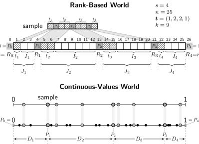
Figure 1: Illustration of the notations used in the analysis; top: quantities that refer to counts (sizes of segments and ranks of elements), bottom: quantities referring to numerical values of certain elements in the model of sorting $n$ i. i. d. $\mathcal{U}(0,1)$ distributed numbers.

We can write the costs with $F_{n}\colonequals F_{n,M_{n}}$ as

$$F_{n} \mathchoice{\mathrel{\;\;{\mathchoice{\mathrel{\overset{\raisebox{0.0pt}{$\scriptstyle\cal D$}}{=}}}{\mathrel{\mathchoice{\hbox{\makebox[10.55551pt][c]{\makebox[0.0pt][c]{$\displaystyle\overset{\raisebox{-4.30554pt}{$\scriptscriptstyle\cal D$}}{=}$}}}}{\hbox{\makebox[10.55551pt][c]{\makebox[0.0pt][c]{$\textstyle\overset{\raisebox{-4.30554pt}{$\scriptscriptstyle\cal D$}}{=}$}}}}{\hbox{\makebox[8.22217pt][c]{\makebox[0.0pt][c]{$\scriptstyle\overset{\raisebox{-3.01389pt}{$\scriptscriptstyle\cal D$}}{=}$}}}}{\hbox{\makebox[6.66661pt][c]{\makebox[0.0pt][c]{$\scriptscriptstyle\overset{\raisebox{-2.15277pt}{$\scriptscriptstyle\cal D$}}{=}$}}}}}}{\mathrel{\overset{\cal D}{=}}}{\mathrel{\overset{\cal D}{=}}}}\;\;}}{\mathrel{\mathchoice{\mathrel{\overset{\raisebox{0.0pt}{$\scriptstyle\cal D$}}{=}}}{\mathrel{\mathchoice{\hbox{\makebox[10.55551pt][c]{\makebox[0.0pt][c]{$\displaystyle\overset{\raisebox{-4.30554pt}{$\scriptscriptstyle\cal D$}}{=}$}}}}{\hbox{\makebox[10.55551pt][c]{\makebox[0.0pt][c]{$\textstyle\overset{\raisebox{-4.30554pt}{$\scriptscriptstyle\cal D$}}{=}$}}}}{\hbox{\makebox[8.22217pt][c]{\makebox[0.0pt][c]{$\scriptstyle\overset{\raisebox{-3.01389pt}{$\scriptscriptstyle\cal D$}}{=}$}}}}{\hbox{\makebox[6.66661pt][c]{\makebox[0.0pt][c]{$\scriptscriptstyle\overset{\raisebox{-2.15277pt}{$\scriptscriptstyle\cal D$}}{=}$}}}}}}{\mathrel{\overset{\cal D}{=}}}{\mathrel{\overset{\cal D}{=}}}}}{\mathrel{\mathchoice{\mathrel{\overset{\raisebox{0.0pt}{$\scriptstyle\cal D$}}{=}}}{\mathrel{\mathchoice{\hbox{\makebox[10.55551pt][c]{\makebox[0.0pt][c]{$\displaystyle\overset{\raisebox{-4.30554pt}{$\scriptscriptstyle\cal D$}}{=}$}}}}{\hbox{\makebox[10.55551pt][c]{\makebox[0.0pt][c]{$\textstyle\overset{\raisebox{-4.30554pt}{$\scriptscriptstyle\cal D$}}{=}$}}}}{\hbox{\makebox[8.22217pt][c]{\makebox[0.0pt][c]{$\scriptstyle\overset{\raisebox{-3.01389pt}{$\scriptscriptstyle\cal D$}}{=}$}}}}{\hbox{\makebox[6.66661pt][c]{\makebox[0.0pt][c]{$\scriptscriptstyle\overset{\raisebox{-2.15277pt}{$\scriptscriptstyle\cal D$}}{=}$}}}}}}{\mathrel{\overset{\cal D}{=}}}{\mathrel{\overset{\cal D}{=}}}}}{\mathrel{\mathchoice{\mathrel{\overset{\raisebox{0.0pt}{$\scriptstyle\cal D$}}{=}}}{\mathrel{\mathchoice{\hbox{\makebox[10.55551pt][c]{\makebox[0.0pt][c]{$\displaystyle\overset{\raisebox{-4.30554pt}{$\scriptscriptstyle\cal D$}}{=}$}}}}{\hbox{\makebox[10.55551pt][c]{\makebox[0.0pt][c]{$\textstyle\overset{\raisebox{-4.30554pt}{$\scriptscriptstyle\cal D$}}{=}$}}}}{\hbox{\makebox[8.22217pt][c]{\makebox[0.0pt][c]{$\scriptstyle\overset{\raisebox{-3.01389pt}{$\scriptscriptstyle\cal D$}}{=}$}}}}{\hbox{\makebox[6.66661pt][c]{\makebox[0.0pt][c]{$\scriptscriptstyle\overset{\raisebox{-2.15277pt}{$\scriptscriptstyle\cal D$}}{=}$}}}}}}{\mathrel{\overset{\cal D}{=}}}{\mathrel{\overset{\cal D}{=}}}}}A_{\mathcal{F}}(n)\mathchoice{\mathbin{\>{+}\>}}{\mathbin{+}}{\mathbin{+}}{\mathbin{+}}\sum_{\ell=1}^{s}\mathds{1}_{\{R_{\ell-1}^{\smash{(}n\smash{)}}<M_{n}<R_{\ell}^{\smash{(}n\smash{)}}\}}\cdot F_{J_{\ell}^{\smash{(}n\smash{)}}}^{\smash{(}\ell\smash{)}},$$ (5)

where $(F_{j}^{\smash{(}\ell\smash{)}})_{j\in\mathbb{N}}$ are independent copies of $({F_{n}})_{n\in\mathbb{N}}$ for $\ell=1,\ldots,s$, which are also independent of $\bm{\mathbold{J}}^{\smash{(}n\smash{)}}$, $A_{\mathcal{F}}(n)$ and $M_{n}$. This distributional recurrence is of the shape required for the distributional master theorem (DMT) to compute asymptotic approximations for the expected values. We next check the technical conditions for the DMT.

Distribution of Subproblem Sizes

For a single pivot chosen randomly (without pivot sampling) we have $J_{\ell}\mathchoice{\mathrel{\overset{\raisebox{0.0pt}{$\scriptstyle\cal D$}}{=}}}{\mathrel{\mathchoice{\hbox{\makebox[10.55551pt][c]{\makebox[0.0pt][c]{$\displaystyle\overset{\raisebox{-4.30554pt}{$\scriptscriptstyle\cal D$}}{=}$}}}}{\hbox{\makebox[10.55551pt][c]{\makebox[0.0pt][c]{$\textstyle\overset{\raisebox{-4.30554pt}{$\scriptscriptstyle\cal D$}}{=}$}}}}{\hbox{\makebox[8.22217pt][c]{\makebox[0.0pt][c]{$\scriptstyle\overset{\raisebox{-3.01389pt}{$\scriptscriptstyle\cal D$}}{=}$}}}}{\hbox{\makebox[6.66661pt][c]{\makebox[0.0pt][c]{$\scriptscriptstyle\overset{\raisebox{-2.15277pt}{$\scriptscriptstyle\cal D$}}{=}$}}}}}}{\mathrel{\overset{\cal D}{=}}}{\mathrel{\overset{\cal D}{=}}}\mathcal{U}[0..n-1]$, a discrete uniform distribution. In general, we have two summands: $J_{\ell}=t_{\ell}+I_{\ell}$. The first one accounts for the part of the sample that belongs to the $\ell$th subproblem, which is a deterministic contribution dictated by the sampling scheme. $I_{\ell}$ is the number of elements that were not part of the sample and were found to belong to the $\ell$th segment in the partitioning step. $I_{\ell}$ is a random variable, and its distribution is $I_{\ell}\mathchoice{\mathrel{\overset{\raisebox{0.0pt}{$\scriptstyle\cal D$}}{=}}}{\mathrel{\mathchoice{\hbox{\makebox[10.55551pt][c]{\makebox[0.0pt][c]{$\displaystyle\overset{\raisebox{-4.30554pt}{$\scriptscriptstyle\cal D$}}{=}$}}}}{\hbox{\makebox[10.55551pt][c]{\makebox[0.0pt][c]{$\textstyle\overset{\raisebox{-4.30554pt}{$\scriptscriptstyle\cal D$}}{=}$}}}}{\hbox{\makebox[8.22217pt][c]{\makebox[0.0pt][c]{$\scriptstyle\overset{\raisebox{-3.01389pt}{$\scriptscriptstyle\cal D$}}{=}$}}}}{\hbox{\makebox[6.66661pt][c]{\makebox[0.0pt][c]{$\scriptscriptstyle\overset{\raisebox{-2.15277pt}{$\scriptscriptstyle\cal D$}}{=}$}}}}}}{\mathrel{\overset{\cal D}{=}}}{\mathrel{\overset{\cal D}{=}}}\mathrm{BetaBin}(n-k,t_{\ell}+1,k-t_{\ell})$, a so-called beta-binomial distribution.

The connection to the beta distribution is best seen by assuming $n$ independent and uniformly in $(0,1)$ distributed reals as input. They are almost surely pairwise distinct and their relative ranking is a random permutation of $[n]$, so this assumption is w. l. o. g. for our analysis. Then, the $\ell$th subproblem contains all elements between $P_{\ell-1}$ and $P_{\ell}$, $\ell=1,\ldots,s$. The spacing $D_{\ell}\colonequals P_{\ell}-P_{\ell-1}$ has a $\mathrm{Beta}(t_{\ell}+1,k-t_{\ell})$ distribution (by definition!), and conditional on that spacing $I_{\ell}\mathchoice{\mathrel{\overset{\raisebox{0.0pt}{$\scriptstyle\cal D$}}{=}}}{\mathrel{\mathchoice{\hbox{\makebox[10.55551pt][c]{\makebox[0.0pt][c]{$\displaystyle\overset{\raisebox{-4.30554pt}{$\scriptscriptstyle\cal D$}}{=}$}}}}{\hbox{\makebox[10.55551pt][c]{\makebox[0.0pt][c]{$\textstyle\overset{\raisebox{-4.30554pt}{$\scriptscriptstyle\cal D$}}{=}$}}}}{\hbox{\makebox[8.22217pt][c]{\makebox[0.0pt][c]{$\scriptstyle\overset{\raisebox{-3.01389pt}{$\scriptscriptstyle\cal D$}}{=}$}}}}{\hbox{\makebox[6.66661pt][c]{\makebox[0.0pt][c]{$\scriptscriptstyle\overset{\raisebox{-2.15277pt}{$\scriptscriptstyle\cal D$}}{=}$}}}}}}{\mathrel{\overset{\cal D}{=}}}{\mathrel{\overset{\cal D}{=}}}\mathrm{Bin}(n-k,D_{\ell})$ has a binomial distribution: Once the pivot values $P_{\ell-1}$ and $P_{\ell}$ are fixed, any element falls between them with probability $D_{\ell}$. The resulting mixture is the so-called beta-binomial distribution. Note that for $\bm{\mathbold{t}}=0$, $t_{\ell}+\mathrm{BetaBin}(n-k,t_{\ell}+1,k-t_{\ell})=\mathrm{BetaBin}(n-1,1,s-1)$ which coincides with $\mathcal{U}[0..n-1]$ for $s=2$.

Convergence of Relative Subproblem Sizes

In light of the stochastic representation of the beta-binomial distribution, we know that conditional on $D_{\ell}$, $Z_{\ell}=I_{\ell}^{\smash{(}n\smash{)}}/n$ is concentrated around $D_{\ell}$. Bounding the errors carefully yields the required local limit law for the relative subproblem size $Z_{\ell}$: By Lem.​ 2.1, we find that Equation (2) is satisfied with $\delta=1$ and the limiting density $f_{Z_{\ell}^{*}}(z)=z^{t_{\ell}}(1-z)^{k-t_{\ell}-1}/\mathrm{B}(t_{\ell}+1,k-t_{\ell})$, which is the density of the $\mathrm{Beta}(t_{\ell}+1,k-t_{\ell})$ distribution. $f_{Z_{\ell}^{*}}$ is clearly Lipschitz (and hence Hölder) continuous on $[0,1]$ since its derivative is bounded in $[0,1]$, so the conditions of the DMT are fulfilled.

Conditional Convergence of Coefficients

For the second condition, Equation (3), we have to consider the distribution of $[R_{\ell-1}<M_{n}<R_{\ell}]$ conditional on the relative subproblem size $J_{\ell}^{\smash{(}n\smash{)}}/n$ for the $\ell$th recursive call. Since $M_{n}$ is uniformly distributed, only the number of choices for $M_{n}$ in the considered range $[R_{\ell-1}<M_{n}<R_{\ell}]$ is important: $R_{\ell}-R_{\ell-1}-1=J_{\ell}$. So we have $\mathbb{P}\big{[}R_{\ell-1}^{\smash{(}n\smash{)}}<M_{n}<R_{\ell}^{\smash{(}n\smash{)}}\nonscript\>\big{|}\nonscript\>\mathopen{}J_{\ell}^{\smash{(}n\smash{)}}\big{]}\mathchoice{\mathrel{\;\;{=}\;\;}}{\mathrel{=}}{\mathrel{=}}{\mathrel{=}}\frac{J_{\ell}^{\smash{(}n\smash{)}}}{n},$ so Equation (3) is fulfilled with $a_{\ell}(z)=z$ and $\delta=1$. $f_{Z_{\ell}^{*}}(z)\cdot a_{\ell}(z)$ is Lipschitz and hence Hölder-continuous as required.

Solution for linear toll functions

We can hence apply the master theorem. The $Z_{\ell}^{*}$ from Thm.​ 2.4 correspond exactly to our spacings $D_{\ell}\mathchoice{\mathrel{\overset{\raisebox{0.0pt}{$\scriptstyle\cal D$}}{=}}}{\mathrel{\mathchoice{\hbox{\makebox[10.55551pt][c]{\makebox[0.0pt][c]{$\displaystyle\overset{\raisebox{-4.30554pt}{$\scriptscriptstyle\cal D$}}{=}$}}}}{\hbox{\makebox[10.55551pt][c]{\makebox[0.0pt][c]{$\textstyle\overset{\raisebox{-4.30554pt}{$\scriptscriptstyle\cal D$}}{=}$}}}}{\hbox{\makebox[8.22217pt][c]{\makebox[0.0pt][c]{$\scriptstyle\overset{\raisebox{-3.01389pt}{$\scriptscriptstyle\cal D$}}{=}$}}}}{\hbox{\makebox[6.66661pt][c]{\makebox[0.0pt][c]{$\scriptscriptstyle\overset{\raisebox{-2.15277pt}{$\scriptscriptstyle\cal D$}}{=}$}}}}}}{\mathrel{\overset{\cal D}{=}}}{\mathrel{\overset{\cal D}{=}}}\mathrm{Beta}(t_{\ell}+1,k-t_{\ell})$. We have $\mathbb{E}[A_{\mathcal{F}}(n)]\sim a_{\mathcal{F}}\cdot n$ with $a_{\mathcal{F}}$ a constant depending on the method and $\mathcal{F}$. So $\alpha=1$ and $\beta=0$ and we compute

$$H \mathchoice{\mathrel{\;{=}\;}}{\mathrel{=}}{\mathrel{=}}{\mathrel{=}}1-\sum_{\ell=1}^{s}\mathbb{E}\big{[}D_{\ell}^{\alpha}\,a_{\ell}(D_{\ell})\big{]}\mathchoice{\mathrel{\;{=}\;}}{\mathrel{=}}{\mathrel{=}}{\mathrel{=}}1-\sum_{\ell=1}^{s}\mathbb{E}\big{[}D_{\ell}^{2}\big{]}$$

$$\mathchoice{\mathrel{\;{=}\;}}{\mathrel{=}}{\mathrel{=}}{\mathrel{=}}1-\sum_{\ell=1}^{s}\frac{(t_{\ell}+1)^{\overline{2}}}{(k+1)^{\overline{2}}}.$$

Since $\frac{(t_{\ell}+1)^{\overline{2}}}{(k+1)^{\overline{2}}}<\frac{t_{\ell}+1}{k+1}$ and $\sum_{\ell=1}^{s}\frac{t_{\ell}+1}{k+1}=1$, we have $H>0$. So by Case 1, we find $\mathbb{E}[F_{n}]\mathchoice{\mathrel{\;\;{\sim}\;\;}}{\mathrel{\sim}}{\mathrel{\sim}}{\mathrel{\sim}}\frac{a_{\mathcal{F}}}{H}\cdot n.$

4.1 Generic Multiway Partitioning

The partitioning methods of practical relevance – classic Hoare-Sedgewick partitioning ($s=2$) [35], Lomuto partitioning [5] ($s=2$), YBB partitioning ($s=3$) [19] and “Waterloo partitioning” ($s=4$) [27] – have been generalized to arbitrary $s$ and analyzed in [39, Chapter 5] with respect to the expected number of comparisons, scanned elements and write accesses. By using the respective values for $a_{\mathcal{F}}$ given in [39, Thm. 7.1] in the asymptotic expression for $\mathbb{E}[F_{n}]$, we obtain the overall costs for selecting random ranks; (see Tab.​ 1 for some results).

4.2 Discussion

Although the results for generic $s$-way partitioning are readily available we refrain from stating them in full generality since the expressions are lengthy and many variants are not promising for selection. Intuitively, a large $s$ can hardly be useful when we always recurse into only a single subproblem.

$s$ Name $\mathbb{E}[C_{n}]/n$ $\mathbb{E}[\mathit{SE}_{n}]/n$ $\mathbb{E}[\mathit{WA}_{n}]/n$ $2$ classic $3$ $3$ $1$ $3$ YBB $3.1\overline{6}$ $2.\overline{6}$ $1.8\overline{3}$ $4$ Waterloo $3.\overline{3}$ $2.5$ $2$ $5$ $3.5$ $2.7$ $2.35$ $6$ $3.\overline{6}$ $2.8$ $2.5\overline{3}$ $7$ $3.7\overline{857142}$ $3.\overline{047619}$ $2.8\overline{3}$ $8$ $3.\overline{857142}$ $3.2\overline{142857}$ $3.03\overline{571428}$

Table 1: The coefficient of the linear term of the expected number of comparisons, scanned elements and write accesses to the array for Quickselect with $s$-way partitioning without pivot sampling ($\bm{\mathbold{t}}=0$) when searching a random rank (“grand averages”).

The optimal number of pivots

Tab.​ 1 confirms this intuition; indeed for the classical cost measures of key comparisons ($C_{n}$) and write access ($\mathit{WA}_{n}$, related to key exchanges) there is no improvement whatsoever from multiway partitioning in Quickselect (as pointed out before [41]). In terms of scanned elements ($\mathit{SE}_{n}$), however, significant savings are observed. Here, Tab.​ 1 contains a surprise: the minimum for scanned elements is attained for $s=4$! This is against the intuition since there will always be (at least) two adjacent segments whose subdivision was fruitless. How can this possibly be better than avoiding the extra work to produce a fourth segment?

The answer is that $s=4$ is indeed suboptimal; but our comparison in Tab.​ 1 is not quite fair. We do not select pivots from a sample, but the multiway methods do have to sort their $s-1$ pivots to operate correctly. We therefore allow multiway methods to enjoy pivots of better quality compared to methods with smaller $s$, thus giving the former an undue advantage. This unfairness is inherent in any such comparison (as previously noticed in the context of sorting [39, 40]).

Simulation by binary partitioning

A fair evaluation of the usefulness of multiway partitioning is nevertheless possible by considering the following (hypothetical) Quickselect variant: We select pivots as we would for the $s$-way method, but then use several rounds of classic single-pivot partitioning to obtain the same segments as with one round of the $s$-way method. For example, the four segments produced by Waterloo partitioning could also be obtained by first partitioning around the middle pivot and then the resulting left resp. right segment around the small resp. large pivot. Note that the first round uses the median of three elements (the middle pivot), whereas the second round effectively runs with pivots selected uniformly from their subrange. By comparing the cost of both variants, we truly evaluate the quality of the partitioning methods since they use the same pivot values.

Comparing Waterloo partitioning with its simulation, we observe that both execute exactly the same set of comparisons, but w. r. t. scanned elements, the simulation scans each element twice. Waterloo partitioning scans all elements once and only the elements in the outer two segments a second time (an average of $1.5n$ vs. $2n$ scanned elements). This clearly exposes the superiority of multiway partitioning in terms of cache behavior and explains its advantage for sorting.

In Quickselect, we will only pursue one subproblem recursively. The simulation of Waterloo partitioning subdivides both segments resulting from the first split, even though one will be knowingly useless! We should therefore compare Waterloo select to a binary simulation without the useless second subdivision. The number of scanned elements then is $n$ for the first round, plus the size of the segment on which we apply the second subdivision. The probability to subdivide the left resp. right resulting segment is the relative size of that segment (the probability that the random rank lies there). The partitioning costs are hence $n+\mathbb{E}[(J_{1}+J_{2})^{2}/n]+\mathbb{E}[(J_{3}+J_{4})^{2}/n]\sim 1.6n$ (for $\bm{\mathbold{t}}=(0,0,0,0)$), and the total cost are given by $\mathit{SE}_{n}\sim 1.6n/H(0,0,0,0)=2.\overline{6}$. This is still higher than $2.5n$, but much closer than $3n$. That Waterloo-select performs so much better than classic Quickselect according to Tab.​ 1 is thus mostly due to the use of a median-of-3 pivot for the first partitioning round, and only to a smaller extent due to its inherent advantage in terms of scanned elements.

We next consider YBB partitioning. Its simulation first partitions around the larger pivot and then subdivide the left segment around the smaller pivot. This “atomic” version would incur $3.\overline{3}n$ scanned elements, much more than the $2.\overline{6}n$ of YBB-Select and indeed more than the $3n$ for classic Quickselect. But for the lucky case that the sought pivot falls into the rightmost segment, the second subdivision is not needed and should be skipped; this lazy version incurs on average $n+\mathbb{E}[(J_{1}+J_{2})^{2}/n]\sim 1.5n$ scanned elements per partitioning step and thus still $1.5n/H(0,0,0)=3n$ scanned elements in total.

Two pivots are optimal!

But how does YBB-select compare to Waterloo-select? A simulation of one by the other does not seem sensible, but we can use the pivots for Waterloo-select (three random elements in order, $\bm{\mathbold{t}}=(0,0,0,0)$) in YBB-select. Ignoring the largest pivot and doing the three-way split using YBB-partitioning corresponds to YBB-select with $\bm{\mathbold{t}}=(0,0,1)$, which needs $\sim 2.5n$ scanned elements, the same as Waterloo-select.

This statement is also true when we let Waterloo-select choose pivots equidistantly from a sample: If $\bm{\mathbold{t}}=(t,t,t,t)$ (for any $t\in\mathbb{N}_{0}$), the expected number of scanned elements is $\sim\frac{4t+5}{2t+2}n$. Selecting pivots the same way, discarding the largest and using YBB-partitioning with the two smaller pivots yields the same asymptotic result. Of course, Waterloo-select performs more comparisons and array accesses to achieve this, so we can conclude that when scanned elements dominate costs, dual-pivot partitioning is the unique optimum choice for Quickselect!

Summary

Splitting the input into several segments at the same time saves memory transfers. While this unconditionally helps in sorting, the game is different in selection where only one subproblem is considered recursively. The flexibility to postpone the decision which part of the input should be further partitioned (and hence the possibility to avoid the splitting of any discarded segments) outperforms the savings in scanned elements from multiway partitioning. Dual-pivot partitioning is an exception, though, since all splits were useful when we recurse into the middle segment.

4.3 Adaptive Methods

All the methods discussed above are non-adaptive: they only take the value of $m$ into account when they decide which subproblem to recurse into. Unfortunately, this is an inherent limitation of the single-parameter recurrence that we use. The validity of the recurrence relies on randomness preservation for $m$: apart from the which subproblem contains the $m$th smallest element, nothing has been learned about the rank of this element within the subproblem. Conditioned on the event that the sought rank is found in the given subproblem, its rank is still uniformly distributed within the subproblem.

For adaptive methods, this is different. Since partitioning costs and subproblem size distribution depend on the $v$ for which $\alpha\in I_{v}$, we inevitably learn which interval $\alpha$ lies in, in addition to the index of subproblem on which we recurse. So even if $m$ is originally uniformly distributed in $[n]$, for recursive calls it is known to lie in a smaller range. The grand average costs of adaptive Quickselect hence do not follow a simple one-parameter recurrence.

5 Asymptotic Approximation for Linear Ranks

We now consider selecting a fixed $\alpha$-quantile, where $\alpha\in(0,1)$ is a parameter of the analysis. We start with the distributional equation (4) and take expectations on both sides. Since we expect the overall costs to be asymptotically linear, we divide by $n$:

$$\frac{\mathbb{E}[F_{n,m}]}{n}\mathchoice{\mathrel{\;\;{=}\;\;}}{\mathrel{=}}{\mathrel{=}}{\mathrel{=}}\frac{\mathbb{E}[A_{\mathcal{F}}(n,m)]}{n}\mathchoice{\mathbin{\;{+}\;}}{\mathbin{+}}{\mathbin{+}}{\mathbin{+}}\mkern-17.0mu\sum_{1\leq\underline{r}<\overline{r}\leq n}\mkern-10.0mu\frac{\overline{r}-\underline{r}-1}{n}\times{}\\ \Biggl{(}\sum_{\ell=1}^{s}\mathbb{P}\big{[}(R_{\ell-1},R_{\ell})=(\underline{r},\overline{r})\big{]}\Biggr{)}\cdot\frac{\mathbb{E}[F_{\overline{r}-\underline{r}-1,m-\underline{r}}]}{\overline{r}-\underline{r}-1}.$$

Thm.​ 5.1 below confirms (under very general conditions) that passing to the limit in this recurrence yields the desired asymptotic approximation.

This has been proven for single-pivot Quickselect even in a stochastic sense [15, 16]; the used techniques can be extended to adaptive methods as outlined in [29]. We give an elementary proof that covers generic $s$-way Quickselect and interestingly seems not to appear in the literature. The details are a bit lengthy and deferred to Appendix F, but we do not need any sophisticated machinery: We simply use the ansatz $\mathbb{E}[F_{n,m}]\sim f(\frac{m}{n})n$ to obtain an educated guess for $f$ and bound the error $\bigl{|}\mathbb{E}[F_{n,m}]-f(\frac{m}{n})n\bigr{|}$. The latter fulfills a similar recurrence as $\mathbb{E}[F_{n,m}]$, but with a much smaller toll function. A crude bound suffices for the claim.

Theorem 5.1 (Convergence Linear Ranks):

Consider generic (adaptive) Quickselect (as defined in §​ 2.4) and assume $\mathbb{E}[A_{\mathcal{F}}(n,m)]=a_{\mathcal{F}}(\frac{m}{n})n\mathchoice{\mathbin{\>{\pm}\>}}{\mathbin{\pm}}{\mathbin{\pm}}{\mathbin{\pm}}O(1)$. Let $f:[0,1]\to\mathbb{R}_{\geq}0$ be a function that fulfills the following integral equation:

$$f(\alpha)\mathchoice{\mathrel{\;{=}\;}}{\mathrel{=}}{\mathrel{=}}{\mathrel{=}}a_{\mathcal{F}}(\alpha)$$ (6)

$$\phantom{=}\mathchoice{\mathbin{\>{+}\>}}{\mathbin{+}}{\mathbin{+}}{\mathbin{+}}\frac{1}{\mathrm{B}\bigl{(}(t_{1},\underrightarrow{t_{1}})+1\bigr{)}}\int_{u=\alpha}^{1}\mkern-10.0muu^{t_{1}+1}(1-u)^{\underrightarrow{t_{1}}}f\Bigl{(}\frac{\alpha}{u}\Bigr{)}\,du$$

$$\phantom{=}\mathchoice{\mathbin{\>{+}\>}}{\mathbin{+}}{\mathbin{+}}{\mathbin{+}}\frac{1}{\mathrm{B}\bigl{(}(t_{s},\underleftarrow{t_{s}})+1\bigr{)}}\int_{v=0}^{\alpha}\mkern-10.0muv^{\underleftarrow{t_{s}}}(1-v)^{t_{s}+1}f\Bigl{(}\frac{\alpha-v}{1-v}\Bigr{)}\,dv$$

$$\phantom{=}\mathchoice{\mathbin{\>{+}\>}}{\mathbin{+}}{\mathbin{+}}{\mathbin{+}}\sum_{\ell=2}^{s-1}\frac{1}{\mathrm{B}\bigl{(}(\underleftarrow{t_{\ell}},t_{\ell},\underrightarrow{t_{\ell}})+1\bigr{)}}\times{}$$

$$\phantom{=}\int_{u=0}^{\alpha}\int_{v=\alpha}^{1}\mkern-10.0muu^{\underleftarrow{t_{\ell}}}(v-u)^{t_{\ell}+1}(1-v)^{\underrightarrow{t_{\ell}}}f\Bigl{(}\frac{\alpha-u}{v-u}\Bigr{)}\,dv\,du,$$

where we abbreviate $\underleftarrow{t_{\ell}}\mathchoice{\mathrel{\;\;{=}\;\;}}{\mathrel{=}}{\mathrel{=}}{\mathrel{=}}\sum_{r=1}^{\ell-1}(t_{r}+1)\mathchoice{\mathbin{\>{-}\>}}{\mathbin{-}}{\mathbin{-}}{\mathbin{-}}1\text{ and }\underrightarrow{t_{\ell}}\mathchoice{\mathrel{\;\;{=}\;\;}}{\mathrel{=}}{\mathrel{=}}{\mathrel{=}}\sum_{r=\ell+1}^{s}(t_{r}+1)\mathchoice{\mathbin{\>{-}\>}}{\mathbin{-}}{\mathbin{-}}{\mathbin{-}}1$. For adaptive methods, $s$ and $\bm{\mathbold{t}}$ are functions of $\alpha$, which is suppressed for legibility. Then (6) is required piecewise for $\alpha\in I_{v}$, $v\in[d]$.

Assume that $f$ is “(piecewise) smooth”, i. e., $f$ (restricted to $I_{v}$) is Hölder-continuous with exponent $h\in(0,1]$ (for all $v\in[d]$). Then the limit $\lim_{n\to\infty;\frac{m}{n}\to\alpha}{\mathbb{E}[F_{n,m}]}/{n}$ exists for $\alpha\in(0,1)\setminus\mathcal{A}$, where $\mathcal{A}$ is the set of boundaries of $I_{1},\ldots,I_{d}$.

Moreover, with $m=\lceil\alpha n\rceil$ holds

$$\mathbb{E}[F_{n,m}] \mathchoice{\mathrel{\;\;{=}\;\;}}{\mathrel{=}}{\mathrel{=}}{\mathrel{=}}f(\tfrac{m}{n})n\mathchoice{\mathbin{\;{\pm}\;}}{\mathbin{\pm}}{\mathbin{\pm}}{\mathbin{\pm}}O(n^{1-2h/3}),\quad(n\to\infty).$$

Our continuity requirements for $f$ may appear restrictive, but they are fulfilled in all examples we studied. They might indeed follow from (6) in general, but we do not attempt to prove this conjecture.

How to obtain $f$

Equation (6) determines $f$ only implicitly. Our route to an explicit expression consists of the following steps. 1) Use substitutions to obtain integrals that only involve $f(x)$ instead of the shifted and scaled arguments. 2) Take successive derivatives on both sides until all integrals vanish. This will result in a higher-order differential equation for $f$ that we aim to solve. 3) Compute $f$ by determining constants of integration from boundary conditions and known results (e. g., symmetry and results for $\alpha\to 0$ and random ranks).

Separable equations for adaptive sampling

Since taking derivatives does not change the argument of $f$, the differential equation will only relate different derivatives of $f$ evaluated at the same point $x$. This is vital for adaptive sampling since it means that we can solve the differential equation for each $I_{v}$ separately. Only step 3) involves the interactions of the regimes.

We remark that we can obtain the leading-term coefficient of the grand average by integrating: $\bar{f}\mathchoice{\mathrel{\;\;{=}\;\;}}{\mathrel{=}}{\mathrel{=}}{\mathrel{=}}\int_{0}^{1}f(\alpha)\,d\alpha$. This also works for adaptive methods.

The discussion in §​ 4 justifies a restriction to $s\leq 3$ segments, but an explicit solution for the differential equation seems out of reach for the general case. We therefore focus on the simplest special cases first.

6 YBB-Select with Linear Ranks

As a warm-up, and part of our main result on Sesquickselect, we consider YBB-Select (YQS) without sampling (as studied in [41]). We start with (6) and substitute $x\mapsto\alpha/u$, $x\mapsto\frac{\alpha-v}{1-v}$ and $x\mapsto\frac{\alpha-u}{v-u}$ in the first, second and third integral, respectively. Simplifying the integrals is fairly standard; we show details for the most interesting one:

$$\mkern 0.0mu\int_{v=0}^{\alpha}\int_{v=\alpha}^{1}(v-u)f\Bigl{(}\frac{\alpha-u}{v-u}\Bigr{)}\,dv\,du$$

$$\mathchoice{\mathrel{\;{=}\;}}{\mathrel{=}}{\mathrel{=}}{\mathrel{=}}\int_{v=0}^{\alpha}(v-\alpha)^{2}\int_{x=0}^{\alpha/v}\frac{f(x)}{(1-x)^{3}}\,dx\,dv$$

$$\mathchoice{\mathrel{\;{=}\;}}{\mathrel{=}}{\mathrel{=}}{\mathrel{=}}\int_{x=0}^{1}\frac{f(x)}{(1-x)^{3}}\int_{v=\alpha}^{\min\{1,\frac{\alpha}{x}\}}(v-\alpha)^{2}\,dv\,dx$$

$$\mathchoice{\mathrel{\;{=}\;}}{\mathrel{=}}{\mathrel{=}}{\mathrel{=}}\frac{(1-\alpha)^{3}}{3}\mkern-4.0mu\int_{x=0}^{\alpha}\frac{f(x)}{(1-x)^{3}}\,dx\mathchoice{\mathbin{\>{+}\>}}{\mathbin{+}}{\mathbin{+}}{\mathbin{+}}\frac{\alpha^{3}}{3}\mkern-3.0mu\int_{x=\alpha}^{1}\mkern-7.0mu\frac{f(x)}{x^{3}}\,dx.$$

Inserting yields the integral equation for $\bm{\mathbold{t}}=(0,0,0)$,

$$f(\alpha) \mathchoice{\mathrel{\>{=}\>}}{\mathrel{=}}{\mathrel{=}}{\mathrel{=}}a_{\mathcal{F}}(\alpha)\mathchoice{\mathbin{\>{+}\>}}{\mathbin{+}}{\mathbin{+}}{\mathbin{+}}$$ (7)

$$\mathchoice{\mathrel{\>{\phantom{=}}\>}}{\mathrel{\phantom{=}}}{\mathrel{\phantom{=}}}{\mathrel{\phantom{=}}}2\Biggl{(}\alpha^{2}\int_{\alpha}^{1}\frac{f(x)}{x^{3}}\,dx\mathchoice{\mathbin{\>{-}\>}}{\mathbin{-}}{\mathbin{-}}{\mathbin{-}}\alpha^{3}\int_{\alpha}^{1}\frac{f(x)}{x^{4}}\,dx$$

$$\mathchoice{\mathrel{\>{\phantom{=}}\>}}{\mathrel{\phantom{=}}}{\mathrel{\phantom{=}}}{\mathrel{\phantom{=}}}\mathchoice{\mathbin{\>{+}\>}}{\mathbin{+}}{\mathbin{+}}{\mathbin{+}}(1-\alpha)^{2}\mkern-4.0mu\int_{0}^{\alpha}\mkern-7.0mu\frac{f(x)\,dx}{(1-x)^{3}}-(1-\alpha)^{3}\mkern-4.0mu\int_{0}^{\alpha}\mkern-7.0mu\frac{f(x)\,dx}{(1-x)^{4}}$$

$$\mathchoice{\mathrel{\>{\phantom{=}}\>}}{\mathrel{\phantom{=}}}{\mathrel{\phantom{=}}}{\mathrel{\phantom{=}}}\mathchoice{\mathbin{\>{+}\>}}{\mathbin{+}}{\mathbin{+}}{\mathbin{+}}\frac{(1-\alpha)^{3}}{3}\mkern-5.0mu\int_{0}^{\alpha}\mkern-7.0mu\frac{f(x)}{(1-x)^{3}}\,dx\mathchoice{\mathbin{\>{+}\>}}{\mathbin{+}}{\mathbin{+}}{\mathbin{+}}\frac{\alpha^{3}}{3}\mkern-3.0mu\int_{\alpha}^{1}\mkern-3.0mu\frac{f(x)}{x^{3}}\,dx\Biggr{)},$$

and taking derivatives four times yields

$$\frac{d^{4}f}{d\alpha^{4}}\mathchoice{\mathrel{\;\;{=}\;\;}}{\mathrel{=}}{\mathrel{=}}{\mathrel{=}}\frac{d^{4}a_{\mathcal{F}}}{d\alpha^{4}}\mathchoice{\mathbin{\>{+}\>}}{\mathbin{+}}{\mathbin{+}}{\mathbin{+}}2\cdot\frac{1-3\alpha(1-\alpha)}{\alpha^{2}(1-\alpha)^{2}}\cdot\frac{d^{2}f}{d\alpha^{2}}.$$ (8)

For comparisons $a_{\mathcal{C}}(\alpha)=19/12$ and for scanned elements $a_{\mathcal{SE}}(\alpha)=4/3$. More generally, if $a_{\mathcal{F}}(\alpha)=a$ for some constant $a$ we can solve (8) to get

$$f(\alpha) \mathchoice{\mathrel{\;{=}\;}}{\mathrel{=}}{\mathrel{=}}{\mathrel{=}}C_{1}+C_{2}\cdot\alpha$$

$$\mathchoice{\mathrel{\;{\phantom{=}}\;}}{\mathrel{\phantom{=}}}{\mathrel{\phantom{=}}}{\mathrel{\phantom{=}}}{}+C_{3}\cdot\left(1-(1-\alpha)\ln(1-\alpha)-\alpha\ln(\alpha)\right)$$

$$\mathchoice{\mathrel{\;{\phantom{=}}\;}}{\mathrel{\phantom{=}}}{\mathrel{\phantom{=}}}{\mathrel{\phantom{=}}}{}+C_{4}\Bigl{(}\tfrac{3}{10}\alpha^{5}-\tfrac{3}{4}\alpha^{4}+\tfrac{1}{6}\alpha^{3}+\tfrac{1}{2}\alpha^{2}$$

$$\mathchoice{\mathrel{\;{\phantom{=}}\;}}{\mathrel{\phantom{=}}}{\mathrel{\phantom{=}}}{\mathrel{\phantom{=}}}\quad\qquad{}-(1-\alpha)\ln(1-\alpha)+1-\alpha\Bigr{)}$$

for some constants $C_{i}$, $i=1,\ldots,4$, to be determined. If $a_{\mathcal{F}}(\alpha)$ is symmetric, that is, $a_{\mathcal{F}}(\alpha)=a_{\mathcal{F}}(1-\alpha)$ for any $\alpha\in[0,1]$ then $f(\alpha)$ is also symmetric, and this entails $C_{2}=C_{4}=0$. Therefore $f(\alpha)=C_{1}+C_{3}\cdot(1+h(\alpha))$ where $h(\alpha)=-(1-\alpha)\ln(1-\alpha)-\alpha\ln(\alpha)$. We have $a_{\mathcal{F}}(\alpha)=a$ for some constant $a$, and from §​ 4, we then know $\overline{f}=2a$. Moreover, we can also determine $\mathbb{E}[F_{n,1}]$ with the DMT (see also [41]) and find $f(0)=3a_{\mathcal{F}}(0)/2$ (this equality holds in terms of right limits when $\alpha\to 0^{+}$). These two equations determine $C_{1}$ and $C_{3}$ and we obtain

$$f^{[\mathrm{YQS}]}(\alpha)\mathchoice{\mathrel{\;{=}\;}}{\mathrel{=}}{\mathrel{=}}{\mathrel{=}}a^{[\mathrm{YQS}]}\left(\frac{3}{2}+h(\alpha)\right).$$ (9)

Recall that for standard quickselect $f^{[\mathrm{CQS}]}(\alpha)=a^{[\mathrm{CQS}]}(2+2h(x))$ (§​ 1.1). We stress here that the values for $a$ are different for CQS and YQS.

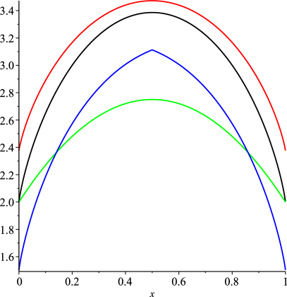
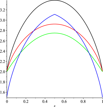
Figure 2: Key comparions, $c(\alpha)$, (left) and scanned elements, $\mathit{se}(\alpha)$, (right) for standard Quickselect (black), YBB-select (red), median-of-three Quickselect (green) and proportion-from-2 (blue).

Discussion

Classic Quickselect (CQS) uses fewer comparisons than YBB-Select (YQS) not only in the grand average, but for any fixed relative rank, (see Fig.​ 2 left). Similarly for write accesses, which we omit due to space constraints. For scanned elements, however, YQS scans less elements on average than CQS for any relative rank $\alpha$, (Fig.​ 2 right)! The difference $\mathit{se}^{[\mathrm{CQS}]}(\alpha)-\mathit{se}^{[\mathrm{YQS}]}(\alpha)=\frac{2}{3}h(\alpha)$ is positive for all $\alpha\in(0,1)$ and reaches a maximum of about $13.6\%$ more at $\alpha=1/2$ (approx. $3.386$ vs. $2.924$). As we know from §​ 4 (Tab.​ 1), $\overline{se}^{[\mathrm{CQS}]}=3$ and $\overline{se}^{[\mathrm{YQS}]}=2.\overline{6}$, i. e., on average for random ranks, YQS scans $11.1\%$ less elements than CQS.

Fig.​ 2 shows two further Quickselect variants. Median-of-three Quickselect (M3) beats YQS on all ranks, but the comparison is not quite fair because of the larger sample. Proportion-from-2 (PROP2), however, uses the same sample size as YQS: It selects the smaller resp. larger of two sampled elements depending on whether $\alpha\leq 1/2$ or $\alpha>1/2$ holds. This adaptive variant was considered in [29]; it is optimal w. r. t. comparisons for sample size 2 and beats YQS w. r. t. scanned elements for extremal $\alpha$ (roughly when $\alpha\leq 0.281$ or $\alpha\geq 0.719$) and grand average ($\overline{\mathit{se}}^{[\mathrm{PROP2}]}\approx 2.598$). The dual-pivot equivalent of proportion-from-2 that we study next will improve on this significantly.

7 Sesquickselect

Like PROP2, Sesquickselect (SQS) uses two sample elements. If $\alpha<\nu$ for a parameter $\nu\in[0,\frac{1}{2}]$, we use the smaller element in the sample to partition the array, if $\alpha>1-\nu$ use the larger element, and if $\alpha\in[\nu,1-\nu]$ use both elements as pivots in YBB partitioning. We now analyze Sesquickselect on linear ranks following the same steps as in §​ 6.

Provided $f(\alpha)=\lim_{n\to\infty,m/n\to\alpha}\mathbb{E}\left[{F_{n,m}}\right]/n$ exists (recall §​ 5), it will be a piecewise-defined function: $f(\alpha)=f_{1}(\alpha)$ for $\alpha\in I_{1}\colonequals[0,\nu)$, $f(\alpha)=f_{2}(\alpha)$ for $\alpha\in I_{2}\colonequals[\nu,1-\nu]$, and $f(\alpha)=f_{3}(\alpha)$ for $\alpha\in I_{3}\colonequals(1-\nu,1]$. Moreover, since $a_{\mathcal{F}}(\alpha)$ is symmetric (i. e., $a_{\mathcal{F}}(\alpha)=a_{\mathcal{F}}(1-\alpha)$) so is $f(\alpha)$, which implies $f_{3}(\alpha)=f_{1}(1-\alpha)$ and $f_{2}(\alpha)=f_{2}(1-\alpha)$. Only two “pieces”, say $f_{1}$ and $f_{2}$, thus have to be determined. For $f_{2}(\alpha)$, we find that it satisfies the very same differential equation, (8), as $f^{[\mathrm{YQS}]}$. This is not surprising; $f_{2}$ is the YQS branch of SQS and the differential equation only uses local properties of $f$ (as pointed out in §​ 5). And inside $I_{2}$, $f=f_{2}$.

Likewise, $f_{1}(\alpha)$ satisfies the same differential equation as the function $f_{1}$ in PROP2 (see [29]):

$$\frac{d^{4}f_{1}}{d\alpha^{4}} \mathchoice{\mathrel{\;{=}\;}}{\mathrel{=}}{\mathrel{=}}{\mathrel{=}}\frac{d^{4}a_{\mathcal{F}}}{d\alpha^{4}}\mathchoice{\mathbin{\>{+}\>}}{\mathbin{+}}{\mathbin{+}}{\mathbin{+}}\frac{2}{\alpha^{2}}\cdot\frac{d^{2}f_{1}}{d\alpha^{2}}\mathchoice{\mathbin{\>{+}\>}}{\mathbin{+}}{\mathbin{+}}{\mathbin{+}}\frac{2}{(1-\alpha)}\cdot\frac{d^{3}f_{1}}{d\alpha^{3}}.$$

The derivatives of $a_{\mathcal{F}}(\alpha)$ vanish (inside any $I_{v}$), and we can reduce the order of both differential equations using $\phi_{1}=f_{1}^{\prime\prime}$ and $\phi_{2}=f_{2}^{\prime\prime}$. This yields

$$f_{1}(x) \mathchoice{\mathrel{\;{=}\;}}{\mathrel{=}}{\mathrel{=}}{\mathrel{=}}C_{1}\Bigl{(}\tfrac{1}{6}x^{3}+\tfrac{1}{2}x^{2}-x-(1-x)\ln(1-x)\Bigr{)}$$

$$\mathchoice{\mathrel{\;{\phantom{=}}\;}}{\mathrel{\phantom{=}}}{\mathrel{\phantom{=}}}{\mathrel{\phantom{=}}}\mathchoice{\mathbin{\>{+}\>}}{\mathbin{+}}{\mathbin{+}}{\mathbin{+}}C_{2}h(x)\mathchoice{\mathbin{\>{+}\>}}{\mathbin{+}}{\mathbin{+}}{\mathbin{+}}C_{3}x\mathchoice{\mathbin{\>{+}\>}}{\mathbin{+}}{\mathbin{+}}{\mathbin{+}}C_{6},$$

$$f_{2}(\alpha) \mathchoice{\mathrel{\;{=}\;}}{\mathrel{=}}{\mathrel{=}}{\mathrel{=}}C_{4}\mathchoice{\mathbin{\>{+}\>}}{\mathbin{+}}{\mathbin{+}}{\mathbin{+}}C_{5}h(x),$$

for constants $C_{1},\ldots,C_{6}$ that depend on the cost measure and threshold $\nu$. We will write $f(\alpha)=f_{\nu}(\alpha)$ resp. $\nu$-SQS to stress this latter dependence. The symmetry of $f_{2}$ was already taken into account. Since $f_{1}(0)=\frac{3}{2}a_{\mathcal{F}}(0)$ we can eliminate $C_{6}=\frac{3}{2}a_{\mathcal{F}}(0)$. To determine the remaining constants, we insert the general expression for $f_{1}$ and $f_{2}$ into the integral equation and equate. The process is laborious, but doable with computer algebra; we report explicit expressions for $C_{1},\ldots,C_{5}$ for comparisons and scanned elements in Appendix D.

Discussion

We will focus on scanned elements. To understand how $\nu$-SQS behaves for different $\nu$, we consider $g_{1}(\nu)=\lim_{\alpha\to\nu^{-}}f_{1,\nu}(\alpha)$ and $g_{2}(\nu)=\lim_{\alpha\to\nu^{+}}f_{2,\nu}(\alpha)$, the values of the two branches of $f_{\nu}$ at $\nu$. We have $g_{1}(0)=\lim_{\nu\to 0^{+}}g_{1}(\nu)=1.\overline{6}$ and $g_{2}(0)=\lim_{\nu\to 0^{+}}g_{2}(\nu)=2$, but $g_{1}(\frac{1}{2})\approx 3.11$ and $g_{2}(\frac{1}{2})\approx 2.91$ Since $g_{1}$ and $g_{2}$ are continuous and strictly increasing for $\nu\in(0,\frac{1}{2})$, they cross at a unique point $\nu=\nu^{\ast}\in(0,\frac{1}{2})$. This point is indeed the right choice:

Theorem 7.1 (Optimal Sesquickselect):

There exists an optimal value of $\nu^{\ast}\approx 0.265\,717$ such that $se_{1,\nu^{\ast}}(\nu^{\ast})=se_{2,\nu^{\ast}}(\nu^{\ast})$. $\nu^{*}$-SQS scans fewer elements than other $\nu$-SQS, i. e., $se_{\nu^{\ast}}(\alpha)\leq se_{\nu}(\alpha),$ for all $\nu\in[0,\frac{1}{2}]$ and all $\alpha\in[0,1]$; in particular, $se_{\nu^{\ast}}(\alpha)\leq se^{[\mathrm{YQS}]}(\alpha)$ and $se_{\nu^{\ast}}(\alpha)\leq se^{[\mathrm{PROP2}]}(\alpha)$ for any $\alpha\in[0,1]$.

The proof is similar to [29, Thm 5.1], we give the details in Appendix E.

Since $\nu^{\ast}$ is optimum across all relative ranks, $\nu^{\ast}$ minimizes $se_{\nu}(1/2)$ and $\overline{se}_{\nu}$: we have $se_{\nu^{\ast}}(1/2)\approx 2.843$ and $\overline{se}_{\nu^{\ast}}\approx 2.5004$, (see also Tab.​ 2).

Comparisons Scanned elements $\alpha$ PROP2 YQS $\nu^{*}$-SQS YQS $\nu^{*}-$SQS $0$ $1.5$ $2.375$ $1.5$ $2$ $1.5$ $1/2$ $3.113^{+}$ $3.472^{+}$ $3.252^{+}$ $2.924^{+}$ $2.843^{+}$ avg $2.598^{+}$ $3.1\overline{6}$ $2.733^{+}$ $2.\overline{6}$ $2.500^{+}$

Table 2: Some special values of $c(\alpha)$ ($\overline{c}$) and $se(\alpha)$ ($\overline{se}$) for several variants: YQS ($\nu=0$), PROP2 ($\nu=1/2$) and $\nu^{*}$-SQS. (Recall that $c^{[\mathrm{PROP2}]}=\mathit{se}^{[\mathrm{PROP2}]}$.)

7.1 Sesquickselect with larger samples

The idea of Sesquickselect naturally extends to more than two sample elements: SQS$k$ adaptively chooses one or two elements as pivot(s) from a sample of $k$. (SQS is simply SQS2 in this notation). For larger $k$, there are many options to do this and guidance is needed to select good variants. With pivot sampling, scanned-element costs for YBB partitioning are $a_{\mathcal{SE}}=1+(t_{1}+1)/(k+1)$; when $t_{3}<t_{1}$, we can improve this to $1+(t_{3}+1)/(k+1)$ using “BBY partitioning”, a symmetric variant of YBB partitioning. We hence assume here that $a_{\mathcal{SE}}=1+\frac{\min\{t_{1},t_{3}\}+1}{k+1}$.

We could give a complete analysis for SQS2, but for larger $k$ the higher-order differential equations seem to withstand analytic solutions. We can, however, numerically solve the integral equation (6) to get insight into which adaptive variants are promising algorithms. The code is available online: https://github.com/sebawild/quickselect-integral-equation. Although numeric convergence was very good in all our explorations, we do not prove the validity of the numeric procedures. The smoothness requirement for Thm.​ 5.1 seemed likewise to be fulfilled in all cases, but it remains a working hypothesis for this section.

We conjecture that the variants given in Fig.​ 3 are the (approximately) optimal choices for the given sample size; they have been found by extensive albeit non-exhaustive search. Fig.​ 4 compares the scanned-elements cost for Sesquickselect and biased proportion-from-$k$ for small $k$.

Discussion

We observe that for $k\leq 7$ we are still far away from the optimal leading term of $1+\min\{\alpha,1-\alpha\}$. For example, $\overline{\mathit{se}}^{[\mathrm{SQS7}]}\approx 1.841$, almost 50% more than the optimal $1.25$. This is quite different in sorting, where median-of-7 Quicksort is less than 10% above optimum in the leading term.

A possible explanation is that the variance of the pivot ranks is too big. Consider, e. g., $k=7$ and $\alpha\in[0.465,0.5]$. The probability to recurse on the middle segment for, e. g., $\bm{\mathbold{t}}=(2,0,3)$ is only roughly $1$%. We must therefore use rather balanced sampling vectors (here $\bm{\mathbold{t}}=(1,2,2)$) and thus lose the ability to reduce the problem size to much less than $\frac{1}{3}n$ in one step.

Figure 3: Our conjectured (approx.) optimal SQS$k$ variants for small $k$. If $\alpha$ falls in the interval (delimited by the values given below the line), the vector above the line is used for $\bm{\mathbold{t}}$. When $\bm{\mathbold{t}}$ has two entries, classic partitioning is used; where three entries are given, we use YBB-partitioning for $\alpha\leq\frac{1}{2}$ and BBY-partitioning for $\alpha>\frac{1}{2}$.

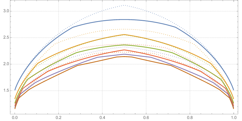
Figure 4: $\mathit{se}(\alpha)$ for SQS$k$ (thick) and (optimally biased) PROP$k$ (dotted) for $k=2$ (blue), $k=3$ (yellow), $k=4$ (green), $k=5$ (red), $k=6$ (purple), and $k=7$ (brown).

8 Conclusion

Despite the asymptotic optimality of the Floyd-Rivest algorithm, practical implementations use Quickselect variants with a fixed-size sample. Since they hence look very similar to sorting methods based on Quicksort, it is tempting to copy optimizations that fair well in sorting blindly to the selection routines. However, our results show that the similarities are misleading. While multiway partitioning is vital in Quicksort for saving memory transfers – a cost measure of increasing relevance – more than two pivots are not helpful in Quickselect.

Moreover, Quickselect offers a large potential for optimization that has no counterpart in sorting whatsoever: adapting the strategy to the (relative) sought rank $\alpha=\frac{m}{n}$. The biased proportion-from-$k$ variants of single-pivot Quickselect proposed in [29] minimize the number of comparisons; in terms of scanned elements, however, Sesquickselect – a novel combination of single-pivot and dual-pivot Quickselect – outperforms proportion-from-$k$ significantly.

In the limit for large sample sizes $k\to\infty$, Sesquickselect converges to the Floyd-Rivest algorithm. This limit is “degenerate” in that we always choose two pivots (Sesquickselect only uses a single pivot for extreme $\alpha$), and that the middle segment has size $o(n)$ (in expectation). In that case, also the savings of dual-pivot partitioning over its simulation by two binary partitioning rounds are negligible.

For practical sample sizes, one cannot rely on this connection to design a good selection method, though – unlike for single-pivot variants, mimicking Floyd-Rivest too closely can result in performance much worse than non-adaptive Quickselect. We need analyses that explicitly take the effect of fixed-size samples into account; such are initiated in this article.

8.1 Future Work

We had to leave many interesting questions about Sesquickselect open; some are not even known for single-pivot Quickselect.

• How fast do the costs converge to the optimum as $k$ grows? Only an upper bound for median-of-$k$ seems known [15, Thm. 4].

• In Fig.​ 3, the number of intervals seems to grow linearly with $k$; can we avoid the use of many different versions in adaptive methods while still achieving (close to) optimal costs?

• Do the theoretical improvements translate to faster running time? Preliminary explorations were promising although the relative improvements are small.

• What is the order of the second term / the speed of convergence in the asymptotic expansion of the costs for fixed quantiles?

• How does adaptive sampling affect the variance, higher moments or full distribution of costs? Some results for PROP$k$ are shown in [23].

• Does adaptive sampling also improve the number of symbol comparisons?

Appendix

.0.0AppendixAppendix.0 Sesquickselect: One and a half pivots for cache-efficient selection

Appendix A Index of Notation

In this appendix, we collect the notations used in this work.

A.1 Generic Mathematical Notation

• natural numbers $\mathbb{N}=\{1,2,3,\ldots\}$, $\mathbb{N}_{0}=\mathbb{N}\cup\{0\}$, integers $\mathbb{Z}=\{\ldots,-2,-1,0,1,2,\ldots\}$, rational numbers $\mathbb{Q}=\{p/q:p\in\mathbb{Z}\wedge q\in\mathbb{N}\}$, real numbers $\mathbb{R}$, and complex numbers $\mathbb{C}$.

• restricted sets $X_{\mathrm{pred}}=\{x\in X:x\text{ fulfills }\mathrm{pred}\}$.

• repeating decimal; $0.\overline{3}=0.333\ldots=\frac{1}{3}$;
  numerals under the line form the repeated part of the decimal number.

• natural and binary logarithm; $\ln(n)=\log_{e}(n)$, $\operatorname{ld}(n)=\log_{2}(n)$.

• to emphasize that $\bm{\mathbold{x}}$ is a vector, it is written in bold;
  components of the vector are not written in bold: $\bm{\mathbold{x}}=(x_{1},\ldots,x_{d})$;
  unless stated otherwise, all vectors are column vectors.

• directed limits; $\lim_{x\to a^{+}f(x)}$ is $\lim_{n\to\infty}f(a+\varepsilon_{n})$ and $\lim_{x\to a^{-}f(x)}$ is $\lim_{n\to\infty}f(a-\varepsilon_{n})$ for a strictly positive sequence $(\varepsilon_{n})_{n\in\mathbb{N}}$ with $\lim_{n\to\infty}\varepsilon_{n}=0$.

• to emphasize that $X$ is a random variable it is Capitalized.

• real intervals, the end points with round parentheses are excluded, those with square brackets are included.

• integer intervals, $[m..n]=\{m,m+1,\ldots,n\}$; $[n]=[1..n]$.

• Iverson bracket, $[\text{stmt}]=1$ if stmt is true, $[\text{stmt}]=0$ otherwise.

• $p$-norm; for $\bm{\mathbold{x}}\in\mathbb{R}^{d}$ and $p\in\mathbb{R}_{\geq 1}$ we have $\|\bm{\mathbold{x}}\|_{p}=\bigl{(}\sum_{r=1}^{d}|x_{r}|\bigr{)}^{1/p}$.

• $\infty$-norm or maximum-norm; for $\bm{\mathbold{x}}\in\mathbb{R}^{d}$ we have $\|\bm{\mathbold{x}}\|_{\infty}=\max_{r=1,\ldots,d}|x_{r}|$.

• element-wise application on vectors; $(x_{1},\ldots,x_{d})+1=(x_{1}+1,\ldots,x_{d}+1)$ and $2^{\bm{\mathbold{x}}}=(2^{x_{1}},\ldots,2^{x_{d}})$; for any function $f:\mathbb{C}\to\mathbb{C}$ write $f(\bm{\mathbold{x}})=(f(x_{1}),\ldots,f(x_{d}))$ etc.

• “total” of a vector; for $\bm{\mathbold{x}}=(x_{1},\ldots,x_{d})$, we have $\Sigma\bm{\mathbold{x}}=\sum_{i=1}^{d}x_{i}$.

• $n$th harmonic number; $H_{n}=\sum_{i=1}^{n}1/i$.

• asymptotic notation as defined, e. g., by [11, Section A.2]; $f=g\pm O(h)$ is equivalent to $|f-g|\in O(|h|)$.

• the gamma function, $\Gamma(z)=\int_{0}^{\infty}t^{z-1}e^{-t}\,dt$.

• $d$-dimensional beta function $\mathrm{B}(\alpha_{1},\ldots,\alpha_{d})=\prod_{i=1}^{d}\Gamma(\alpha_{i})/\Gamma(\alpha+\beta)$.

• factorial powers notation of Graham et al. [13];
  “$a$ to the $b$ falling resp. rising.”

• the binary base-$e$ entropy function $h(x)=-x\ln(x)-(1-x)\ln(1-x)$.

• abbreviation for a polynomial with given coefficients; $\mathopen{\langle\!\langle}{a_{n},\ldots,a_{0}}\mathclose{\rangle\!\rangle}=a_{n}\nu^{n}+a_{n-1}\nu^{n-1}+\cdots+a_{1}\nu+a_{0}$. (used in Appendix D).

A.2 Stochastics-related Notation

• probability of an event $E$ resp. probability for random variable $X$ to attain value $x$.

• expected value of $X$; I write $\mathbb{E}[X\nonscript\>|\nonscript\>\mathopen{}Y]$ for the conditional expectation of $X$ given $Y$, and $\mathbb{E}_{#1}[f(X)]$ to emphasize that expectation is taken w. r. t. random variable $X$.

• equality in distribution; $X$ and $Y$ have the same distribution.

• indicator variable for event $E$, i. e., $\mathds{1}_{E}$ is $1$ if $E$ occurs and $0$ otherwise; $\{X\leq 5\}$ denotes the event induced by the expression $X\leq 5$.

• uniformly in $(a,b)\subset\mathbb{R}$ distributed random variable.

• discrete uniformly in $[a..b]\subset\mathbb{Z}$ distributed random variable.

• beta distributed random variable with shape parameters $\alpha\in\mathbb{R}_{>0}$ and $\beta\in\mathbb{R}_{>0}$. $X\mathchoice{\mathrel{\overset{\raisebox{0.0pt}{$\scriptstyle\cal D$}}{=}}}{\mathrel{\mathchoice{\hbox{\makebox[9.50002pt][c]{\makebox[0.0pt][c]{$\displaystyle\overset{\raisebox{-3.87498pt}{$\scriptscriptstyle\cal D$}}{=}$}}}}{\hbox{\makebox[9.50002pt][c]{\makebox[0.0pt][c]{$\textstyle\overset{\raisebox{-3.87498pt}{$\scriptscriptstyle\cal D$}}{=}$}}}}{\hbox{\makebox[7.40001pt][c]{\makebox[0.0pt][c]{$\scriptstyle\overset{\raisebox{-2.7125pt}{$\scriptscriptstyle\cal D$}}{=}$}}}}{\hbox{\makebox[6.0pt][c]{\makebox[0.0pt][c]{$\scriptscriptstyle\overset{\raisebox{-1.93748pt}{$\scriptscriptstyle\cal D$}}{=}$}}}}}}{\mathrel{\overset{\cal D}{=}}}{\mathrel{\overset{\cal D}{=}}}\mathrm{Beta}(\alpha,\beta)$ is equivalent to $(X,1-X)\mathchoice{\mathrel{\overset{\raisebox{0.0pt}{$\scriptstyle\cal D$}}{=}}}{\mathrel{\mathchoice{\hbox{\makebox[9.50002pt][c]{\makebox[0.0pt][c]{$\displaystyle\overset{\raisebox{-3.87498pt}{$\scriptscriptstyle\cal D$}}{=}$}}}}{\hbox{\makebox[9.50002pt][c]{\makebox[0.0pt][c]{$\textstyle\overset{\raisebox{-3.87498pt}{$\scriptscriptstyle\cal D$}}{=}$}}}}{\hbox{\makebox[7.40001pt][c]{\makebox[0.0pt][c]{$\scriptstyle\overset{\raisebox{-2.7125pt}{$\scriptscriptstyle\cal D$}}{=}$}}}}{\hbox{\makebox[6.0pt][c]{\makebox[0.0pt][c]{$\scriptscriptstyle\overset{\raisebox{-1.93748pt}{$\scriptscriptstyle\cal D$}}{=}$}}}}}}{\mathrel{\overset{\cal D}{=}}}{\mathrel{\overset{\cal D}{=}}}\mathrm{Dir}(\alpha,\beta)$.

• Dirichlet distributed random variable; $\bm{\mathbold{\alpha}}\in\mathbb{R}_{>0}^{d}$.

• binomial distributed random variable with $n\in\mathbb{N}_{0}$ trials and success probability $p\in[0,1]$; $X\mathchoice{\mathrel{\overset{\raisebox{0.0pt}{$\scriptstyle\cal D$}}{=}}}{\mathrel{\mathchoice{\hbox{\makebox[9.50002pt][c]{\makebox[0.0pt][c]{$\displaystyle\overset{\raisebox{-3.87498pt}{$\scriptscriptstyle\cal D$}}{=}$}}}}{\hbox{\makebox[9.50002pt][c]{\makebox[0.0pt][c]{$\textstyle\overset{\raisebox{-3.87498pt}{$\scriptscriptstyle\cal D$}}{=}$}}}}{\hbox{\makebox[7.40001pt][c]{\makebox[0.0pt][c]{$\scriptstyle\overset{\raisebox{-2.7125pt}{$\scriptscriptstyle\cal D$}}{=}$}}}}{\hbox{\makebox[6.0pt][c]{\makebox[0.0pt][c]{$\scriptscriptstyle\overset{\raisebox{-1.93748pt}{$\scriptscriptstyle\cal D$}}{=}$}}}}}}{\mathrel{\overset{\cal D}{=}}}{\mathrel{\overset{\cal D}{=}}}\mathrm{Bin}(n,p)$ is equivalent to $(X,n-X)\mathchoice{\mathrel{\overset{\raisebox{0.0pt}{$\scriptstyle\cal D$}}{=}}}{\mathrel{\mathchoice{\hbox{\makebox[9.50002pt][c]{\makebox[0.0pt][c]{$\displaystyle\overset{\raisebox{-3.87498pt}{$\scriptscriptstyle\cal D$}}{=}$}}}}{\hbox{\makebox[9.50002pt][c]{\makebox[0.0pt][c]{$\textstyle\overset{\raisebox{-3.87498pt}{$\scriptscriptstyle\cal D$}}{=}$}}}}{\hbox{\makebox[7.40001pt][c]{\makebox[0.0pt][c]{$\scriptstyle\overset{\raisebox{-2.7125pt}{$\scriptscriptstyle\cal D$}}{=}$}}}}{\hbox{\makebox[6.0pt][c]{\makebox[0.0pt][c]{$\scriptscriptstyle\overset{\raisebox{-1.93748pt}{$\scriptscriptstyle\cal D$}}{=}$}}}}}}{\mathrel{\overset{\cal D}{=}}}{\mathrel{\overset{\cal D}{=}}}\mathrm{Mult}(n;p,1-p)$.

• multinomially distributed random variable; $n\in\mathbb{N}_{0}$ and $\bm{\mathbold{p}}\in[0,1]^{d}$ with $\Sigma\bm{\mathbold{p}}=1$.

• beta-binomial distributed random variable; $n\in\mathbb{N}_{0}$, $\alpha,\beta\in\mathbb{R}_{>0}$; $X\mathchoice{\mathrel{\overset{\raisebox{0.0pt}{$\scriptstyle\cal D$}}{=}}}{\mathrel{\mathchoice{\hbox{\makebox[9.50002pt][c]{\makebox[0.0pt][c]{$\displaystyle\overset{\raisebox{-3.87498pt}{$\scriptscriptstyle\cal D$}}{=}$}}}}{\hbox{\makebox[9.50002pt][c]{\makebox[0.0pt][c]{$\textstyle\overset{\raisebox{-3.87498pt}{$\scriptscriptstyle\cal D$}}{=}$}}}}{\hbox{\makebox[7.40001pt][c]{\makebox[0.0pt][c]{$\scriptstyle\overset{\raisebox{-2.7125pt}{$\scriptscriptstyle\cal D$}}{=}$}}}}{\hbox{\makebox[6.0pt][c]{\makebox[0.0pt][c]{$\scriptscriptstyle\overset{\raisebox{-1.93748pt}{$\scriptscriptstyle\cal D$}}{=}$}}}}}}{\mathrel{\overset{\cal D}{=}}}{\mathrel{\overset{\cal D}{=}}}\mathrm{BetaBin}(n,\alpha,\beta)$ is equivalent to $(X,n-X)\mathchoice{\mathrel{\overset{\raisebox{0.0pt}{$\scriptstyle\cal D$}}{=}}}{\mathrel{\mathchoice{\hbox{\makebox[9.50002pt][c]{\makebox[0.0pt][c]{$\displaystyle\overset{\raisebox{-3.87498pt}{$\scriptscriptstyle\cal D$}}{=}$}}}}{\hbox{\makebox[9.50002pt][c]{\makebox[0.0pt][c]{$\textstyle\overset{\raisebox{-3.87498pt}{$\scriptscriptstyle\cal D$}}{=}$}}}}{\hbox{\makebox[7.40001pt][c]{\makebox[0.0pt][c]{$\scriptstyle\overset{\raisebox{-2.7125pt}{$\scriptscriptstyle\cal D$}}{=}$}}}}{\hbox{\makebox[6.0pt][c]{\makebox[0.0pt][c]{$\scriptscriptstyle\overset{\raisebox{-1.93748pt}{$\scriptscriptstyle\cal D$}}{=}$}}}}}}{\mathrel{\overset{\cal D}{=}}}{\mathrel{\overset{\cal D}{=}}}\mathrm{DirMult}(n;\alpha,\beta)$.

• Dirichlet-multinomial distributed random variable; $n\in\mathbb{N}_{0}$, $\bm{\mathbold{\sigma}}\in\mathbb{R}_{>0}^{s}$.

A.3 Notation for our Analysis

Some notations for the analysis are exemplified in Fig.​ 1 (page 1).

• length of the input array, i. e., the input size.

• the rank to select, $m\in[1..n]$.

• relative sought rank, $\alpha=m/n\in[\frac{1}{n},1]\subset[0,1]$.

• number of segments, $s\geq 2$; determines the number of pivots to be $s-1$. For adaptive methods, $s$ depends on $\alpha$.

• pivot-sampling parameter; $\bm{\mathbold{t}}\in\mathbb{N}^{s}$; see Fig.​ 1. For adaptive methods, $\bm{\mathbold{t}}$ depends on $\alpha$.

• sample size $k\in\mathbb{N}_{\geq s-1}$; $k+1=\Sigma(\bm{\mathbold{t}}+1)$. For adaptive methods, $k$ depends on $\alpha$ (via $\bm{\mathbold{t}}$).

• quantiles vector for sampling, $\bm{\mathbold{\tau}}=\frac{\bm{\mathbold{t}}+1}{k+1}$; we have $\mathbb{E}[D_{\ell}]=\tau_{\ell}$.

• cost measures; $\mathcal{F}$ is the generic placeholder for an arbitrary cost measure, $\mathcal{C}$ means number of comparisons, $\mathcal{SE}$ means number of scanned elements, $\mathcal{WA}$ means number of write accesses to the array.

• (random) costs in the respective cost measure to select the $m$th smallest out of $n$ elements.

• (random) costs (in the respective cost measure) to select a uniform random rank $M_{n}\mathchoice{\mathrel{\overset{\raisebox{0.0pt}{$\scriptstyle\cal D$}}{=}}}{\mathrel{\mathchoice{\hbox{\makebox[9.50002pt][c]{\makebox[0.0pt][c]{$\displaystyle\overset{\raisebox{-3.87498pt}{$\scriptscriptstyle\cal D$}}{=}$}}}}{\hbox{\makebox[9.50002pt][c]{\makebox[0.0pt][c]{$\textstyle\overset{\raisebox{-3.87498pt}{$\scriptscriptstyle\cal D$}}{=}$}}}}{\hbox{\makebox[7.40001pt][c]{\makebox[0.0pt][c]{$\scriptstyle\overset{\raisebox{-2.7125pt}{$\scriptscriptstyle\cal D$}}{=}$}}}}{\hbox{\makebox[6.0pt][c]{\makebox[0.0pt][c]{$\scriptscriptstyle\overset{\raisebox{-1.93748pt}{$\scriptscriptstyle\cal D$}}{=}$}}}}}}{\mathrel{\overset{\cal D}{=}}}{\mathrel{\overset{\cal D}{=}}}\mathcal{U}[1..m]$ out of $n$ elements.

• leading-term coefficient of $\mathbb{E}[F_{n,m}]$ for $n\to\infty$ and $m/n\to\alpha$: $f(\alpha)\mathchoice{\mathrel{\;\;{=}\;\;}}{\mathrel{=}}{\mathrel{=}}{\mathrel{=}}\lim_{{n\to\infty,\frac{m}{n}\to\alpha}}\frac{\mathbb{E}[F_{n,m}]}{n}$;
  similarly for specific cost measures.

• leading-term coefficient of grand average $\bar{f}\mathchoice{\mathrel{\;\;{=}\;\;}}{\mathrel{=}}{\mathrel{=}}{\mathrel{=}}\lim_{n\to\infty}\frac{\mathbb{E}[F_{n,M_{n}}]}{n}\mathchoice{\mathrel{\;\;{=}\;\;}}{\mathrel{=}}{\mathrel{=}}{\mathrel{=}}\int_{0}^{1}f(\alpha)\,d\alpha$; similar for specific cost measures.

• (random) costs of the first partitioning step (in the resp. cost measure) when selecting the $m$th smallest out of $n$ elements.
  (Not directly a function of $m$, but indirectly for adaptive methods).

• leading-term coefficient of $\mathbb{E}[A_{\mathcal{F}}(n,m)]$ for $n\to\infty$ with $m/n\to\alpha$. (Not directly a function of $m$, but indirectly for adaptive methods).

• (random) values of chosen pivots in the first partitioning step,
  ordered by value $0\leq P_{1}\leq P_{2}\leq\cdots\leq P_{s-1}\leq 1$;
  $P_{0}\colonequals 0$ and $P_{s}\colonequals 1$ are used for notational convenience.

• (random) ranks of the pivots in the first partitioning step,
  $1\leq R_{1}\leq R_{2}\leq\cdots\leq R_{s-1}\leq n$;
  $R_{0}\colonequals 0$ and $R_{s}\colonequals n+11$ are used for notational convenience.

• (random) vector of subproblem sizes for recursive calls;
  for initial size $n$, we have $\bm{\mathbold{J}}\in\{0,\ldots,n-(s-1)\}^{s}$ with $\Sigma\bm{\mathbold{J}}1=n-(s-1)$.

• (random) vector of segment sizes; for initial size $n$, we have $\bm{\mathbold{I}}\in\{0,\ldots,n-k\}^{s}$ with $\Sigma\bm{\mathbold{I}}=n-k$;
  $\bm{\mathbold{J}}=\bm{\mathbold{I}}+\bm{\mathbold{t}}$ and $\bm{\mathbold{I}}\mathchoice{\mathrel{\overset{\raisebox{0.0pt}{$\scriptstyle\cal D$}}{=}}}{\mathrel{\mathchoice{\hbox{\makebox[9.50002pt][c]{\makebox[0.0pt][c]{$\displaystyle\overset{\raisebox{-3.87498pt}{$\scriptscriptstyle\cal D$}}{=}$}}}}{\hbox{\makebox[9.50002pt][c]{\makebox[0.0pt][c]{$\textstyle\overset{\raisebox{-3.87498pt}{$\scriptscriptstyle\cal D$}}{=}$}}}}{\hbox{\makebox[7.40001pt][c]{\makebox[0.0pt][c]{$\scriptstyle\overset{\raisebox{-2.7125pt}{$\scriptscriptstyle\cal D$}}{=}$}}}}{\hbox{\makebox[6.0pt][c]{\makebox[0.0pt][c]{$\scriptscriptstyle\overset{\raisebox{-1.93748pt}{$\scriptscriptstyle\cal D$}}{=}$}}}}}}{\mathrel{\overset{\cal D}{=}}}{\mathrel{\overset{\cal D}{=}}}\mathrm{DirMult}(n-k,\bm{\mathbold{t}}+1)$; conditional on $\bm{\mathbold{D}}$ we have $\bm{\mathbold{I}}\mathchoice{\mathrel{\overset{\raisebox{0.0pt}{$\scriptstyle\cal D$}}{=}}}{\mathrel{\mathchoice{\hbox{\makebox[9.50002pt][c]{\makebox[0.0pt][c]{$\displaystyle\overset{\raisebox{-3.87498pt}{$\scriptscriptstyle\cal D$}}{=}$}}}}{\hbox{\makebox[9.50002pt][c]{\makebox[0.0pt][c]{$\textstyle\overset{\raisebox{-3.87498pt}{$\scriptscriptstyle\cal D$}}{=}$}}}}{\hbox{\makebox[7.40001pt][c]{\makebox[0.0pt][c]{$\scriptstyle\overset{\raisebox{-2.7125pt}{$\scriptscriptstyle\cal D$}}{=}$}}}}{\hbox{\makebox[6.0pt][c]{\makebox[0.0pt][c]{$\scriptscriptstyle\overset{\raisebox{-1.93748pt}{$\scriptscriptstyle\cal D$}}{=}$}}}}}}{\mathrel{\overset{\cal D}{=}}}{\mathrel{\overset{\cal D}{=}}}\mathrm{Mult}(n-k,\bm{\mathbold{D}})$.

• (random) spacings of the unit interval $(0,1)$ induced by the pivots $P_{1}\,\ldots,P_{s-1}$, i. e., $D_{i}=P_{i}-P_{i-1}$ for $1\leq i\leq s$; $\bm{\mathbold{D}}\mathchoice{\mathrel{\overset{\raisebox{0.0pt}{$\scriptstyle\cal D$}}{=}}}{\mathrel{\mathchoice{\hbox{\makebox[9.50002pt][c]{\makebox[0.0pt][c]{$\displaystyle\overset{\raisebox{-3.87498pt}{$\scriptscriptstyle\cal D$}}{=}$}}}}{\hbox{\makebox[9.50002pt][c]{\makebox[0.0pt][c]{$\textstyle\overset{\raisebox{-3.87498pt}{$\scriptscriptstyle\cal D$}}{=}$}}}}{\hbox{\makebox[7.40001pt][c]{\makebox[0.0pt][c]{$\scriptstyle\overset{\raisebox{-2.7125pt}{$\scriptscriptstyle\cal D$}}{=}$}}}}{\hbox{\makebox[6.0pt][c]{\makebox[0.0pt][c]{$\scriptscriptstyle\overset{\raisebox{-1.93748pt}{$\scriptscriptstyle\cal D$}}{=}$}}}}}}{\mathrel{\overset{\cal D}{=}}}{\mathrel{\overset{\cal D}{=}}}\mathrm{Dir}(\bm{\mathbold{\sigma}})\mathchoice{\mathrel{\overset{\raisebox{0.0pt}{$\scriptstyle\cal D$}}{=}}}{\mathrel{\mathchoice{\hbox{\makebox[9.50002pt][c]{\makebox[0.0pt][c]{$\displaystyle\overset{\raisebox{-3.87498pt}{$\scriptscriptstyle\cal D$}}{=}$}}}}{\hbox{\makebox[9.50002pt][c]{\makebox[0.0pt][c]{$\textstyle\overset{\raisebox{-3.87498pt}{$\scriptscriptstyle\cal D$}}{=}$}}}}{\hbox{\makebox[7.40001pt][c]{\makebox[0.0pt][c]{$\scriptstyle\overset{\raisebox{-2.7125pt}{$\scriptscriptstyle\cal D$}}{=}$}}}}{\hbox{\makebox[6.0pt][c]{\makebox[0.0pt][c]{$\scriptscriptstyle\overset{\raisebox{-1.93748pt}{$\scriptscriptstyle\cal D$}}{=}$}}}}}}{\mathrel{\overset{\cal D}{=}}}{\mathrel{\overset{\cal D}{=}}}\mathrm{Dir}(\bm{\mathbold{t}}+1)$.

• “const-entropy” $H(\bm{\mathbold{t}})=1-\sum_{r=1}^{s}{\frac{{(t_{r}+1)}^{\overline{2}}}{{(k+1)}^{\overline{2}}}}$.

Appendix B Proof of Hölder integration lemma

In this appendix, we prove the error bound on the integral of Hölder-continuous functions.

breakProof 1

Lem.​ 2.3 Let $C$ be the Hölder-constant of $f$. We split the integral into small integrals over hypercubes of side length $\frac{1}{n}$ and use Hölder-continuity to bound the difference to the corresponding summand:

$$\mkern-50.0mu\Biggl{|}\int_{\bm{\mathbold{x}}\in[0,1]^{d}}f(\bm{\mathbold{x}})\,d\bm{\mathbold{x}}\mathchoice{\mathbin{\;{-}\;}}{\mathbin{-}}{\mathbin{-}}{\mathbin{-}}\frac{1}{n^{d}}\!\!\sum_{\bm{\mathbold{i}}\in[0..n-1]^{d}}\!\!\!f(\bm{\mathbold{i}}/n)\Biggr{|}$$

$$\mathchoice{\mathrel{\;\;{=}\;\;}}{\mathrel{=}}{\mathrel{=}}{\mathrel{=}}\sum_{\bm{\mathbold{i}}\in[0..n-1]^{d}}\Biggl{|}\int_{\bm{\mathbold{x}}\in[0,\frac{1}{n}]^{d}+\frac{\bm{\mathbold{i}}}{n}}f(\bm{\mathbold{x}})\,d\bm{\mathbold{x}}\mathchoice{\mathbin{\>{-}\>}}{\mathbin{-}}{\mathbin{-}}{\mathbin{-}}\frac{f(\bm{\mathbold{i}}/n)}{n^{d}}\Biggr{|}$$

$$\mathchoice{\mathrel{\;\;{=}\;\;}}{\mathrel{=}}{\mathrel{=}}{\mathrel{=}}\sum_{\bm{\mathbold{i}}\in[0..n-1]^{d}}\int_{\bm{\mathbold{x}}\in[0,\frac{1}{n}]^{d}+\frac{\bm{\mathbold{i}}}{n}}\bigl{|}f(\bm{\mathbold{x}})-f(\bm{\mathbold{i}}/n)\bigr{|}\,d\bm{\mathbold{x}}$$

$$\mathchoice{\mathrel{\;\;{\leq}\;\;}}{\mathrel{\leq}}{\mathrel{\leq}}{\mathrel{\leq}}\sum_{\bm{\mathbold{i}}\in[0..n-1]^{d}}\int_{\bm{\mathbold{x}}\in[0,\frac{1}{n}]^{d}+\frac{\bm{\mathbold{i}}}{n}}\sqrt{d}C\bigl{\|}\bm{\mathbold{x}}-\tfrac{\bm{\mathbold{i}}}{n}\bigr{\|}^{h}\,d\bm{\mathbold{x}}$$

$$\mathchoice{\mathrel{\;\;{\leq}\;\;}}{\mathrel{\leq}}{\mathrel{\leq}}{\mathrel{\leq}}\sqrt{d}C\sum_{\bm{\mathbold{i}}\in[0..n-1]^{d}}\int_{\bm{\mathbold{x}}\in[0,\frac{1}{n}]^{d}+\frac{\bm{\mathbold{i}}}{n}}\bigl{(}\tfrac{1}{n}\bigr{)}^{h}\,d\bm{\mathbold{x}}$$

$$\mathchoice{\mathrel{\;\;{=}\;\;}}{\mathrel{=}}{\mathrel{=}}{\mathrel{=}}\sqrt{d}Cn^{-h}\int_{\bm{\mathbold{x}}\in[0,1]^{d}}1\,d\bm{\mathbold{x}}$$

$$\mathchoice{\mathrel{\;\;{=}\;\;}}{\mathrel{=}}{\mathrel{=}}{\mathrel{=}}O(n^{-h}).$$

$\Box$

Appendix C Proof of Local Limit Law

In this appendix, we give the proof for the local limit law of the Dirichlet-multinomial distribution. It is a straight-forward generalization of the computation given in [39, Lemma 2.38], but we include it for a self-contained presentation.

breakProof 2 break(Lem.​ 2.1)

Let $\bm{\mathbold{z}}\in(0,1)^{s}$ with $\Sigma\bm{\mathbold{z}}=1$ be arbitrary and write $\bm{\mathbold{i}}=\bm{\mathbold{i}}(\bm{\mathbold{z}})=\lfloor\bm{\mathbold{z}}(n+1)\rfloor\in[0..n]^{s}$ with $\Sigma\bm{\mathbold{i}}=n$. We note for reference that for $\ell\in[s]$ and any constant $c\geq 0$

$$\bigl{(}\tfrac{i_{\ell}}{n}\bigr{)}^{c} \mathchoice{\mathrel{\;\;{=}\;\;}}{\mathrel{=}}{\mathrel{=}}{\mathrel{=}}\biggl{(}\frac{\lfloor z_{\ell}(n+1)\rfloor}{n}\biggr{)}^{\!c}\mathchoice{\mathrel{\;\;{=}\;\;}}{\mathrel{=}}{\mathrel{=}}{\mathrel{=}}\bigl{(}z_{\ell}\pm O(\tfrac{1}{n})\bigr{)}^{c}\mathchoice{\mathrel{\;\;{=}\;\;}}{\mathrel{=}}{\mathrel{=}}{\mathrel{=}}z_{\ell}^{c}\mathchoice{\mathbin{\>{\pm}\>}}{\mathbin{\pm}}{\mathbin{\pm}}{\mathbin{\pm}}O(\tfrac{1}{n}),\qquad(n\to\infty).$$ (10)

Moreover, we use the following property of the gamma function

$$\frac{\Gamma(z+a)}{\Gamma(z+b)} \mathchoice{\mathrel{\;\;{=}\;\;}}{\mathrel{=}}{\mathrel{=}}{\mathrel{=}}z^{a-b}\pm O(z^{a-b-1}),\qquad(z\to\infty),\quad(a,b\text{ constant}).$$ (11)

This follows from Equation (5.11.13) of the DLMF [10]. With these preparations, we compute

$$\mkern-18.0mun^{s-1}\,\mathbb{P}[\bm{\mathbold{I}}^{\smash{(}n\smash{)}}\!=\bm{\mathbold{i}}]$$

$$\mathchoice{\mathrel{\;\;{=}\;\;}}{\mathrel{=}}{\mathrel{=}}{\mathrel{=}}n^{s-1}\binom{n}{\bm{\mathbold{i}}}\frac{\mathrm{B}(\bm{\mathbold{i}}+\bm{\mathbold{\alpha}})}{\mathrm{B}(\bm{\mathbold{\alpha}})}$$

$$\mathchoice{\mathrel{\;\;{=}\;\;}}{\mathrel{=}}{\mathrel{=}}{\mathrel{=}}\frac{n^{s-1}}{\mathrm{B}(\bm{\mathbold{\alpha}})}\cdot\frac{\Gamma(n+1)}{\prod_{\ell=1}^{s}\Gamma(i_{\ell}+1)}\cdot\frac{\prod_{\ell=1}^{s}\Gamma(i_{\ell}+\alpha_{\ell})}{\Gamma(n+\Sigma\bm{\mathbold{\alpha}})}$$

$$\mathchoice{\mathrel{\;\;{=}\;\;}}{\mathrel{=}}{\mathrel{=}}{\mathrel{=}}\frac{n^{s-1}}{\mathrm{B}(\bm{\mathbold{\alpha}})}\cdot\frac{\Gamma(n+1)}{\Gamma(n+\Sigma\bm{\mathbold{\alpha}})}\cdot\prod_{\ell=1}^{s}\frac{\Gamma(i_{\ell}+\alpha_{\ell})}{\Gamma(i_{\ell}+1)}$$

$$\mathchoice{\mathrel{\;\;{\mathrel{\underset{\mathclap{\makebox[0.0pt][c]{\scriptsize\eqref{eq:gamma-function-quotient-rule}}}}{=}}}\;\;}}{\mathrel{\mathrel{\underset{\mathclap{\makebox[0.0pt][c]{\scriptsize\eqref{eq:gamma-function-quotient-rule}}}}{=}}}}{\mathrel{\mathrel{\underset{\mathclap{\makebox[0.0pt][c]{\scriptsize\eqref{eq:gamma-function-quotient-rule}}}}{=}}}}{\mathrel{\mathrel{\underset{\mathclap{\makebox[0.0pt][c]{\scriptsize\eqref{eq:gamma-function-quotient-rule}}}}{=}}}}\frac{n^{s-1}}{\mathrm{B}(\bm{\mathbold{\alpha}})}\cdot n^{1-\Sigma\bm{\mathbold{\alpha}}}\bigl{(}1\pm O(n^{-1})\bigr{)}\cdot\prod_{\ell=1}^{s}\begin{cases*}1&if $\alpha_{\ell}=1$\\ i_{\ell}^{\alpha_{\ell}-1}\pm O(i_{\ell}^{\alpha_{\ell}-2})&if $\alpha_{\ell}\geq 2$\end{cases*}$$

$$\mathchoice{\mathrel{\;\;{=}\;\;}}{\mathrel{=}}{\mathrel{=}}{\mathrel{=}}\frac{1}{\mathrm{B}(\bm{\mathbold{\alpha}})}\cdot\bigl{(}1\pm O(n^{-1})\bigr{)}\cdot\prod_{\ell=1}^{s}\begin{dcases*}1&if $\alpha_{\ell}=1$\\ \bigl{(}\tfrac{i_{\ell}}{n}\bigr{)}^{\alpha_{\ell}-1}\pm O\Bigl{(}\smash{\underbrace{\bigl{(}\tfrac{i_{\ell}}{n}\bigr{)}^{\alpha_{\ell}-2}}_{O(1)}n^{-1}}\Bigr{)}&if $\alpha_{\ell}\geq 2$\end{dcases*}$$

$$\mathchoice{\mathrel{\;\;{\mathrel{\underset{\mathclap{\makebox[0.0pt][c]{\scriptsize\eqref{eq:floor-i-close-zn}}}}{=}}}\;\;}}{\mathrel{\mathrel{\underset{\mathclap{\makebox[0.0pt][c]{\scriptsize\eqref{eq:floor-i-close-zn}}}}{=}}}}{\mathrel{\mathrel{\underset{\mathclap{\makebox[0.0pt][c]{\scriptsize\eqref{eq:floor-i-close-zn}}}}{=}}}}{\mathrel{\mathrel{\underset{\mathclap{\makebox[0.0pt][c]{\scriptsize\eqref{eq:floor-i-close-zn}}}}{=}}}}\frac{1}{\mathrm{B}(\bm{\mathbold{\alpha}})}\cdot\bigl{(}1\pm O(n^{-1})\bigr{)}\cdot\prod_{\ell=1}^{s}\bigl{(}z_{\ell}^{\alpha_{\ell}-1}\pm O(n^{-1})\bigr{)}$$

$$\mathchoice{\mathrel{\;\;{=}\;\;}}{\mathrel{=}}{\mathrel{=}}{\mathrel{=}}\frac{\prod_{\ell=1}^{s}z_{\ell}^{\alpha_{\ell}-1}}{\mathrm{B}(\bm{\mathbold{\alpha}})}\mathchoice{\mathbin{\;{\pm}\;}}{\mathbin{\pm}}{\mathbin{\pm}}{\mathbin{\pm}}O(n^{-1}).$$

This is exactly the density $f_{D}(\bm{\mathbold{z}})$ of the $\mathrm{Dir}(\bm{\mathbold{\alpha}})$ distribution. $\Box$

Appendix D Constants for Sesquickselect

In this appendix, we give the constants for Sesquickselect as functions in $\nu$. With one exception, the expressions are rather unwieldy and we will have to use some shorthand notation to state concisely. Constant $C_{2}(\nu)$ is very simple; for both comparisons and scanned elements we have $C_{2}(\nu)=2$.

In order to express the remaining constants, it will be convenient to introduce the following two auxiliary functions, namely,

$$\Delta(\nu) \mathchoice{\mathrel{\;\;{\colonequals}\;\;}}{\mathrel{\colonequals}}{\mathrel{\colonequals}}{\mathrel{\colonequals}}2\Biggl{(}60\ln(1-\nu)\nu^{6}-360\ln(1-\nu)\nu^{5}-140\nu^{6}+780\ln(1-\nu)\nu^{4}$$

$$\mathchoice{\mathrel{\;\;{\phantom{=}}\;\;}}{\mathrel{\phantom{=}}}{\mathrel{\phantom{=}}}{\mathrel{\phantom{=}}}\qquad{}+480\nu^{5}-840\ln(1-\nu)\nu^{3}-635\nu^{4}+504\ln(1-\nu)\nu^{2}$$

$$\mathchoice{\mathrel{\;\;{\phantom{=}}\;\;}}{\mathrel{\phantom{=}}}{\mathrel{\phantom{=}}}{\mathrel{\phantom{=}}}\qquad{}+428\nu^{3}-168\ln(1-\nu)\nu-156\nu^{2}+24\ln(1-\nu)+24\nu\Biggr{)},$$

and

$$Q_{a}(\nu) \mathchoice{\mathrel{\;\;{\colonequals}\;\;}}{\mathrel{\colonequals}}{\mathrel{\colonequals}}{\mathrel{\colonequals}}(\nu^{4}-4\nu^{3}+4\nu^{2}-2\nu+a)\cdot(1-\nu)^{2}\ln(1-\nu),\qquad(a\in\mathbb{R}).$$

We will also use the shorthand $Q(\nu):=Q_{1/2}(\nu)$.

Comparisons Scanned Elements $C^{\prime}_{1}$ $\mathopen{\langle\!\langle}{20,-120,260,-276,162,-52,7}\mathclose{\rangle\!\rangle}$ $\mathopen{\langle\!\langle}{20,-120,260,-264,144,-40,4}\mathclose{\rangle\!\rangle}$ $C^{\prime}_{3}$ $\begin{multlined}12Q(\nu)(\ln\nu-\ln(1-\nu))\\ +\mathopen{\langle\!\langle}{6,16,-69,70,-24,-2,2}\mathclose{\rangle\!\rangle}\ln(1-\nu)\\ +\mathopen{\langle\!\langle}{-26,92,-125,86,-33,6}\mathclose{\rangle\!\rangle}\nu\ln\nu\\ +\mathopen{\langle\!\langle}{45,-124,121,-52,5,2}\mathclose{\rangle\!\rangle}\nu\end{multlined}12Q(\nu)(\ln\nu-\ln(1-\nu))\\ +\mathopen{\langle\!\langle}{6,16,-69,70,-24,-2,2}\mathclose{\rangle\!\rangle}\ln(1-\nu)\\ +\mathopen{\langle\!\langle}{-26,92,-125,86,-33,6}\mathclose{\rangle\!\rangle}\nu\ln\nu\\ +\mathopen{\langle\!\langle}{45,-124,121,-52,5,2}\mathclose{\rangle\!\rangle}\nu$ $\begin{multlined}48Q(\nu)(\ln\nu-\ln(1-\nu))\\ +\mathopen{\langle\!\langle}{90,-308,510,-560,408,-176,32}\mathclose{\rangle\!\rangle}\ln(1-\nu)\\ +\mathopen{\langle\!\langle}{-110,380,-506,344,-132,24}\mathclose{\rangle\!\rangle}\nu\ln\nu\\ +\mathopen{\langle\!\langle}{45,-40,-125,212,-136,32}\mathclose{\rangle\!\rangle}\nu\end{multlined}48Q(\nu)(\ln\nu-\ln(1-\nu))\\ +\mathopen{\langle\!\langle}{90,-308,510,-560,408,-176,32}\mathclose{\rangle\!\rangle}\ln(1-\nu)\\ +\mathopen{\langle\!\langle}{-110,380,-506,344,-132,24}\mathclose{\rangle\!\rangle}\nu\ln\nu\\ +\mathopen{\langle\!\langle}{45,-40,-125,212,-136,32}\mathclose{\rangle\!\rangle}\nu$ $C^{\prime}_{4}$ $\begin{multlined}-12Q(\nu)\ln(1-\nu)\\ +\mathopen{\langle\!\langle}{168,-956,2031,-2180,1317,-446,65}\mathclose{\rangle\!\rangle}\cdot\\ \ln(1-\nu)\\ -\frac{20}{3}\nu^{9}+30\nu^{8}-\frac{170}{3}\nu^{7}\\ +\frac{1}{6}\mathopen{\langle\!\langle}{-1644,6792,-9409,6514,-2445,390}\mathclose{\rangle\!\rangle}\nu\end{multlined}-12Q(\nu)\ln(1-\nu)\\ +\mathopen{\langle\!\langle}{168,-956,2031,-2180,1317,-446,65}\mathclose{\rangle\!\rangle}\cdot\\ \ln(1-\nu)\\ -\frac{20}{3}\nu^{9}+30\nu^{8}-\frac{170}{3}\nu^{7}\\ +\frac{1}{6}\mathopen{\langle\!\langle}{-1644,6792,-9409,6514,-2445,390}\mathclose{\rangle\!\rangle}\nu$ $\begin{multlined}-48Q(\nu)\ln(1-\nu)\\ +\mathopen{\langle\!\langle}{198,-956,1890,-2000,1236,-440,68}\mathclose{\rangle\!\rangle}\cdot\\ \ln(1-\nu)\\ -\frac{20}{3}\nu^{9}+30\nu^{8}-\frac{170}{3}\nu^{7}\\ +\frac{1}{3}\mathopen{\langle\!\langle}{-456,2352,-3641,2756,-1146,204}\mathclose{\rangle\!\rangle}\nu\end{multlined}-48Q(\nu)\ln(1-\nu)\\ +\mathopen{\langle\!\langle}{198,-956,1890,-2000,1236,-440,68}\mathclose{\rangle\!\rangle}\cdot\\ \ln(1-\nu)\\ -\frac{20}{3}\nu^{9}+30\nu^{8}-\frac{170}{3}\nu^{7}\\ +\frac{1}{3}\mathopen{\langle\!\langle}{-456,2352,-3641,2756,-1146,204}\mathclose{\rangle\!\rangle}\nu$ $C^{\prime}_{5}$ $\begin{multlined}228Q_{15/38}(\nu)\\ +\mathopen{\langle\!\langle}{-534,1828,-2415,1626,-591,90}\mathclose{\rangle\!\rangle}\nu\end{multlined}228Q_{15/38}(\nu)\\ +\mathopen{\langle\!\langle}{-534,1828,-2415,1626,-591,90}\mathclose{\rangle\!\rangle}\nu$ $\begin{multlined}192Q_{3/8}(\nu)\\ +\mathopen{\langle\!\langle}{-450,1540,-2034,1368,-492,72}\mathclose{\rangle\!\rangle}\nu\end{multlined}192Q_{3/8}(\nu)\\ +\mathopen{\langle\!\langle}{-450,1540,-2034,1368,-492,72}\mathclose{\rangle\!\rangle}\nu$

Table D.1: Constants for comparisons and scanned elements in Sesquickselect.

Moreover, we will use the notation $\mathopen{\langle\!\langle}{a_{n},\ldots,a_{0}}\mathclose{\rangle\!\rangle}$ to denote the polynomial of degree $n$

$$a_{n}\nu^{n}+a_{n-1}\nu^{n-1}+\cdots+a_{1}\nu+a_{0}.$$

With all these definitions at hand, the expressions for the constants $C^{\prime}_{i}(\nu)=C_{i}(\nu)\cdot\Delta(\nu)$ are collected in Tab.​ D.1.

Appendix E Optimal Threshold for Sesquickselect

In this appendix, we prove the existance of a unique optimal cutoff $\nu^{*}$.

breakProof 3 break(Thm.​ 7.1)

Given a function $g$ in $[0,1]$ and a value $\nu$, $0\leq\nu\leq 1/2$, consider the following operator

$$\bigl{(}T(g)\bigr{)}(\alpha) \mathchoice{\mathrel{\;\;{=}\;\;}}{\mathrel{=}}{\mathrel{=}}{\mathrel{=}}2\Biggl{(}-\alpha^{3}\int_{\alpha}^{1}\frac{g(x)}{x^{4}}\,dx+\alpha^{2}\int_{\alpha}^{1}\frac{g(x)}{x^{3}}\,dx$$

$$\mathchoice{\mathrel{\;\;{\phantom{=}}\;\;}}{\mathrel{\phantom{=}}}{\mathrel{\phantom{=}}}{\mathrel{\phantom{=}}}\quad{}+(1-\alpha)^{3}\int_{0}^{\alpha}\frac{g(x)}{(1-x)^{4}}\,dx\Biggr{)},\qquad(\alpha<\nu),$$

and

$$\bigl{(}T(g)\bigr{)}(\alpha) \mathchoice{\mathrel{\;\;{=}\;\;}}{\mathrel{=}}{\mathrel{=}}{\mathrel{=}}2\Biggl{(}\alpha^{2}\int_{\alpha}^{1}\frac{g(x)}{x^{3}}\,dx-\alpha^{3}\int_{\alpha}^{1}\frac{g(x)}{x^{4}}\,dx$$

$$\mathchoice{\mathrel{\;\;{\phantom{=}}\;\;}}{\mathrel{\phantom{=}}}{\mathrel{\phantom{=}}}{\mathrel{\phantom{=}}}\quad{}+(1-\alpha)^{2}\int_{0}^{\alpha}\frac{g(x)}{(1-x)^{3}}\,dx-(1-\alpha)^{3}\int_{0}^{\alpha}\frac{g(x)}{(1-x)^{4}}\,dx$$

$$\mathchoice{\mathrel{\;\;{\phantom{=}}\;\;}}{\mathrel{\phantom{=}}}{\mathrel{\phantom{=}}}{\mathrel{\phantom{=}}}\quad{}+\frac{(1-\alpha)^{3}}{3}\int_{0}^{\alpha}\frac{g(x)}{(1-x)^{3}}\,dx+\frac{\alpha^{3}}{3}\int_{\alpha}^{1}\frac{g(x)}{x^{3}}\,dx\Biggr{)},\qquad(\nu\leq\alpha\leq 1-\nu).$$

Notice that the function $f_{\nu}$ for Sesquickselect satisfies $f_{\nu}=a_{\mathcal{F}}+T(f_{\nu})$; it is important to emphasize that the function $a_{\mathcal{F}}$ will depend on $\nu$ since we use single partitioning if $\alpha<\nu$ or $\alpha>1-\nu$, whereas we use YBB partitioning if $\nu\leq\alpha\leq 1-\nu$.

To be more precise, the operator $T$ is defined piecewise: $T=[T_{1,\nu},T_{2,\nu}]$, and we can define it so that for $h=T(g)$, we have $h_{1,\nu}=T_{1,\nu}(g_{1,\nu},g_{2,\nu})$ and $h_{2,\nu}=T_{2,\nu}(g_{1,\nu},g_{2,\nu})$, with $h_{1,\nu}$ being the restriction of $h$ to $[0,\nu)\cup(1-\nu,1]$, $h_{2,\nu}$ the restriction of $h$ to $[\nu,1-\nu]$ and similarly for $g_{1,\nu}$ and $g_{2,\nu}$.

Solving the fix-point equation $f=T(f)$ involves the same steps that we have followed to find the explicit solution for Sesquickselect (the differential equations are identical). But we arrive here to the conclusion that $f=0$ is the unique solution of $f=T(f)$. (Note that the summand $a_{\mathcal{F}}$ is missing in the fix-point equation.)

Let $g_{1}(\nu)=\mathit{se}_{1,\nu}$ and $g_{2}(\nu)=\mathit{se}_{2,\nu}$. Both functions are strictly increasing in $(0,\frac{1}{2})$ since their derivatives with respect to $\nu$ are strictly positive. Moreover, we have $g_{1}(0)=\frac{5}{3}<2=g_{2}(0)$ and $g_{1}(\frac{1}{2})\approx 3.112>2.910\approx g_{2}(\frac{1}{2})$, so they cross at a single point $\nu=\nu^{\ast}$. In other words, there exists a unique solution $\nu^{\ast}$ in $(0,\frac{1}{2})$ to the equation $g_{1}(\nu)=g_{2}(\nu)$.

Taking derivatives with respect to $\nu$ on both sides of $\mathit{se}_{\nu}=a_{\mathcal{SE}}+T(\mathit{se}_{\nu})$ and setting $\nu=\nu^{\ast}$, many terms cancel out because $\mathit{se}_{1,\nu^{\ast}}(\nu^{\ast})=\mathit{se}_{2,\nu^{\ast}}(\nu^{\ast})$ and because of the symmetries $\mathit{se}_{3,\nu}(\alpha)=\mathit{se}_{1,\nu}(1-\alpha)$ and $\mathit{se}_{2,\nu}(\alpha)=\mathit{se}_{2,\nu}(1-\alpha)$, so we conclude

$$\left.\frac{\partial se_{\nu}}{\partial\nu}\right|_{\nu=\nu^{\ast}}\mathchoice{\mathrel{\;\;{=}\;\;}}{\mathrel{=}}{\mathrel{=}}{\mathrel{=}}T\left(\left.\frac{\partial se_{\nu}}{\partial\nu}\right|_{\nu=\nu^{\ast}}\right),$$

and hence, $\left.\partial se_{\nu}/\partial\nu\right|_{\nu=\nu^{\ast}}=0$ for any $\alpha\in[0,1]$.

Computing the second derivative of $\mathit{se}_{\nu}(\alpha)$ with respect to $\alpha$ and setting $\nu=\nu^{\ast}$ shows it is positive for all $\alpha$ in $(0,1)$, so we can conclude that $\nu^{\ast}$ is always a local minimum. In fact, we can show that

$$\left.\frac{\partial^{2}se_{\nu}}{\partial\nu^{2}}\right|_{\nu=\nu^{\ast}}\mathchoice{\mathrel{\;\;{=}\;\;}}{\mathrel{=}}{\mathrel{=}}{\mathrel{=}}\delta(\alpha)+T\left(\left.\frac{\partial^{2}se_{\nu}}{\partial\nu^{2}}\right|_{\nu=\nu^{\ast}}\right),$$

for some function $\delta(\alpha)$ which is strictly positive for all $\alpha\in[0,1]$. To be more precise, $\delta(\alpha)=\delta_{1}(\alpha)$ if $\alpha\in[0,\nu^{\ast})\cup(1-\nu^{\ast},1]$ and $\delta(\alpha)=\delta_{2}(\alpha)$ if $\nu^{\ast}\leq\alpha\leq 1-\nu^{\ast}$; both $\delta_{1}$ and $\delta_{2}$ are strictly positive in the corresponding ranges of $\alpha$. Finally, $\delta>0$ for all $\alpha$ entails that $\left.\partial^{2}\mathit{se}_{\nu}/\partial\nu^{2}\right|_{\nu=\nu^{\ast}}>0$ for all $\alpha$.

The limit values $\nu\to 0$ (YQS) and $\nu\to 1/2$ (PROP2) are not minimum, hence to complete the proof we only need to show that for any fixed value of $\alpha$, $\mathit{se}_{\nu}(\alpha)$ has no other local extrema in $(0,\frac{1}{2})$. So let $\hat{\nu}$ be such that $\left.\partial se_{\nu}/\partial\nu\right|_{\nu=\hat{\nu}}=0$ for some $\hat{\alpha}$. Assume w. l. o. g. that $\alpha\leq\frac{1}{2}$; then if $\hat{\alpha}<\hat{\nu}$ we assume that $\left.\partial\mathit{se}_{1,\nu}/\partial\nu\right|_{\nu=\hat{\nu}}=0$, and if $\alpha>\nu$ then $\left.\partial\mathit{se}_{2,\nu}/\partial\nu\right|_{\nu=\hat{\nu}}=0$. Since $\mathit{se}=a_{\mathcal{SE}}+T(\mathit{se})$ and $\partial a_{\mathcal{SE}}/\partial\nu=0$, we have $\partial\mathit{se}_{\nu}/\partial\nu=\partial T(\mathit{se}_{\nu})/\partial\nu$. Setting $\nu=\hat{\nu}$ on both sides, we arrive at the conclusion that if $\left.\partial se_{\nu}/\partial\nu\right|_{\nu=\hat{\nu}}=0$ for some $\hat{\alpha}$ then we must have $\mathit{se}_{1,\hat{\nu}}(\hat{\nu})=\mathit{se}_{2,\hat{\nu}}(\hat{\nu})$. This implies $\hat{\nu}=\nu^{\ast}$ since – as argued above – the latter is the unique value in $(0,\frac{1}{2})$ with $\mathit{se}_{1,\hat{\nu}}(\hat{\nu})=\mathit{se}_{2,\hat{\nu}}(\hat{\nu})$.  $\Box$

Appendix F Proof of Convergence for Linear Ranks

This appendix gives the details for the proof of Thm.​ 5.1.

F.1 Derivation of the integral equation

We start with the distributional equation (4) and take expectations on both sides.

$$\mathbb{E}[F_{n,m}] \mathchoice{\mathrel{\;\;{=}\;\;}}{\mathrel{=}}{\mathrel{=}}{\mathrel{=}}\mathbb{E}[A_{\mathcal{F}}(n,m)]\mathchoice{\mathbin{\>{+}\>}}{\mathbin{+}}{\mathbin{+}}{\mathbin{+}}\sum_{\ell=1}^{s}\mathbb{E}_{#1}\Big{[}\mathds{1}_{\{R_{\ell-1}<m<R_{\ell}\}}\cdot\mathbb{E}[F_{J_{\ell},m-R_{\ell-1}}\nonscript\>|\nonscript\>\mathopen{}\bm{\mathbold{J}}]\Big{]}.$$ (12)

Unfolding the expectation and simplifying yields

$$\sum_{\ell=1}^{s}\mathbb{E}_{#1}\Big{[}\mathds{1}_{\{R_{\ell-1}<m<R_{\ell}\}}\cdot\mathbb{E}[F_{J_{\ell},m-R_{\ell-1}}\nonscript\>|\nonscript\>\mathopen{}\bm{\mathbold{J}}]\Big{]}\mkern-300.0mu$$

$$\mathchoice{\mathrel{\;\;{=}\;\;}}{\mathrel{=}}{\mathrel{=}}{\mathrel{=}}\sum_{j=1}^{n-1}\sum_{a=1}^{m}\Biggl{(}\sum_{\ell=1}^{s}\mathbb{P}[J_{\ell}=j\wedge m-R_{\ell-1}=a]\Biggr{)}\cdot\mathbb{E}[F_{j,a}]$$

$$\mathchoice{\mathrel{\;\;{=}\;\;}}{\mathrel{=}}{\mathrel{=}}{\mathrel{=}}\sum_{\underline{r}=0}^{m-1}\sum_{\overline{r}=\underline{m}+1}^{n+1}\Biggl{(}\sum_{\ell=1}^{s}\mathbb{P}[R_{\ell-1}=\underline{r}\wedge R_{\ell}=\overline{r}]\Biggr{)}\cdot\mathbb{E}[F_{\overline{r}-\underline{r}-1,m-\underline{r}}].$$

(Note that the extreme values $0$ and $n+1$ for $\underline{r}$ resp. $\overline{r}$ are included to handle the outermost segments $\ell=1$ resp. $\ell=s$ and those with $1<\ell<s$ in uniform way. Eventually, these two cases will have to be distinguished, though, since $R_{1},\ldots,R_{s-1}$ are actual random variables, whereas $R_{0}=0$ and $R_{s+1}=n+1$ are deterministic values.) We can express the joint probabilities $\mathbb{P}[(R_{\ell-1},R_{\ell})=(\underline{r},\overline{r})]$ using the relations between $\bm{\mathbold{R}}$ and $\bm{\mathbold{J}}$ and using the aggregation property of the Dirichlet-multinomial distribution (see, e. g., [39, Lemma 2.37]), but we do not need an explicit expression for now. We are interested in the limit $n,m\to\infty$ with $\frac{m}{n}\to\alpha\in(0,1)$, i. e., we are selecting the $\alpha$-quantile of a large list. Since we expect the overall costs to be asymptotically linear, we divide the recurrence by $n$:

$$\frac{\mathbb{E}[F_{n,m}]}{n} \mathchoice{\mathrel{\;\;{=}\;\;}}{\mathrel{=}}{\mathrel{=}}{\mathrel{=}}\frac{\mathbb{E}[A_{\mathcal{F}}(n,m)]}{n}\mathchoice{\mathbin{\>{+}\>}}{\mathbin{+}}{\mathbin{+}}{\mathbin{+}}\sum_{1\leq\underline{r}<\overline{r}\leq n}\frac{\overline{r}-\underline{r}-1}{n}\times{}$$

$$\mathchoice{\mathrel{\;\;{\phantom{=}}\;\;}}{\mathrel{\phantom{=}}}{\mathrel{\phantom{=}}}{\mathrel{\phantom{=}}}{}\quad\Biggl{(}\sum_{\ell=1}^{s}\mathbb{P}\big{[}(R_{\ell-1},R_{\ell})=(\underline{r},\overline{r})\big{]}\Biggr{)}\cdot\frac{\mathbb{E}[F_{\overline{r}-\underline{r}-1,m-\underline{r}}]}{\overline{r}-\underline{r}-1}.$$ (13)

F.2 Proof of convergence

Thm.​ 5.1 essentially claims that we can take the limit in (13) to obtain a characterizing equation for $f(\alpha)$.

breakProof 4 break(Thm.​ 5.1)

It suffices to prove the asymptotic approximation since it implies the existence of the limit. We first connect Equation (6) (disregarding convergence issues) to the normalized expected costs $\mathbb{E}[F_{n,m}]/n$ and then prove the claimed asymptotic approximation.

We start with the ansatz $\mathbb{E}[F_{n,m}]\sim f(\frac{m}{n})n$ for a function $f:[0,1]\to\mathbb{R}$. Inserting into Equation (13) yields for $\frac{m}{n}\to\alpha$

$$f(\alpha) \mathchoice{\mathrel{\;\;{=}\;\;}}{\mathrel{=}}{\mathrel{=}}{\mathrel{=}}a_{\mathcal{F}}(\alpha)\mathchoice{\mathbin{\>{+}\>}}{\mathbin{+}}{\mathbin{+}}{\mathbin{+}}\sum_{\ell=1}^{s}\int_{\underline{z}=0}^{\alpha}\int_{\overline{z}=\alpha}^{1}(\overline{z}-\underline{z})f_{(P_{\ell-1},P_{\ell})}(\underline{z},\overline{z})\cdot f\Bigl{(}\frac{\alpha-\underline{z}}{\overline{z}-\underline{z}}\Bigr{)}\,d\overline{z}\,d\underline{z},$$ (14)

where

$$\SwapAboveDisplaySkip f_{(P_{\ell-1},P_{\ell})}(\underline{z},\overline{z}) \mathchoice{\mathrel{\;\;{=}\;\;}}{\mathrel{=}}{\mathrel{=}}{\mathrel{=}}\begin{dcases}\delta_{0}(\underline{z})\cdot\frac{\overline{z}^{t_{1}}\,(1-\overline{z})^{\underrightarrow{t_{1}}}}{\mathrm{B}(t_{1}+1,\underrightarrow{t_{1}}+1)},&\ell=0;\\ \frac{\underline{z}^{\underleftarrow{t_{\ell}}}\,(\overline{z}-\underline{z})^{t_{\ell}}\,(1-\overline{z})^{\underrightarrow{t_{\ell}}}}{\mathrm{B}(\underleftarrow{t_{\ell}}+1,t_{\ell}+1,\underrightarrow{t_{\ell}}+1)},&1<\ell<s;\\ \delta_{1}(\overline{z})\cdot\frac{\underline{z}^{\underleftarrow{t_{s}}}\,(1-\overline{z})^{t_{s}}}{\mathrm{B}(\underleftarrow{t_{s}}+1,t_{s}+1)},&\ell=s.\end{dcases}$$

Here we write $\delta_{c}(z)$ for the Dirac-delta function at $c$, the degenerate density of a random variable that deterministically has value $c\in\mathbb{R}$. By separating the leftmost and rightmost cases and inserting $f_{(P_{\ell-1},P_{\ell})}$, we obtain the claimed integral equation for $f$.

Let now $\alpha\in(0,1)\setminus\mathcal{A}$ be fixed and set $m=\lceil\alpha n\rceil$. We consider the quantity $r_{n,m}=\mathbb{E}[F_{n,m}]-f(\frac{m}{n})n$. Inserting the recurrence (12) for $\mathbb{E}[F_{n,m}]$ and the integral equation (14) for $f(\frac{m}{n})$ yields

$$r_{n,m} \mathchoice{\mathrel{\;\;{=}\;\;}}{\mathrel{=}}{\mathrel{=}}{\mathrel{=}}b_{r}(n,m)\cdot n\mathchoice{\mathbin{\>{+}\>}}{\mathbin{+}}{\mathbin{+}}{\mathbin{+}}\sum_{\ell=1}^{s}\mathbb{E}_{#1}\left[\mathds{1}_{\{R_{\ell-1}<m<R_{\ell}\}}\cdot r_{R_{\ell}-R_{\ell-1}-1,m-R_{\ell-1}}\right]$$ (15)

with

$$b_{r}(n,m) \mathchoice{\mathrel{\;\;{=}\;\;}}{\mathrel{=}}{\mathrel{=}}{\mathrel{=}}a_{\mathcal{F}}(\tfrac{m}{n})\mathchoice{\mathbin{\>{\pm}\>}}{\mathbin{\pm}}{\mathbin{\pm}}{\mathbin{\pm}}O(n^{-1})-a_{\mathcal{F}}(\alpha)$$

$$\mathchoice{\mathrel{\;\;{\phantom{=}}\;\;}}{\mathrel{\phantom{=}}}{\mathrel{\phantom{=}}}{\mathrel{\phantom{=}}}\quad{}\mathchoice{\mathbin{\>{+}\>}}{\mathbin{+}}{\mathbin{+}}{\mathbin{+}}\sum_{\ell=1}^{s}\sum_{\underline{r}=0}^{m-1}\sum_{\overline{r}=m+1}^{n+1}\!\!\frac{\overline{r}-\underline{r}-1}{n}\cdot\mathbb{P}[R_{\ell-1}=\underline{r}\wedge R_{\ell}=\overline{r}]\cdot f\biggl{(}\frac{m-\underline{r}}{\overline{r}-\underline{r}-1}\biggr{)}$$

$$\mathchoice{\mathrel{\;\;{\phantom{=}}\;\;}}{\mathrel{\phantom{=}}}{\mathrel{\phantom{=}}}{\mathrel{\phantom{=}}}\quad{}\mathchoice{\mathbin{\>{-}\>}}{\mathbin{-}}{\mathbin{-}}{\mathbin{-}}\sum_{\ell=1}^{s}\int_{\underline{z}=0}^{\alpha}\int_{\overline{z}=\alpha}^{1}(\overline{z}-\underline{z})f_{(P_{\ell-1},P_{\ell})}(\underline{z},\overline{z})\cdot f\Bigl{(}\frac{\alpha-\underline{z}}{\overline{z}-\underline{z}}\Bigr{)}\,d\overline{z}\,d\underline{z}.$$

The outline of the remainder of the proof is to first show that $b_{r}(n,m)$ is small, namely $b_{r}(n,m)=O(n^{-2h/3})$, uniformly in $\alpha$. For that we show that the difference above is essentially the difference of an integral and the corresponding Riemann sum. Since the integrand is sufficiently smooth, we can bound the absolute value of this difference, but some case distinctions will be necessary for that. Finally, we show that small $b_{r}(n,m)$ implies that also $r_{n,m}$ is small thus completing the proof.

First of all, not that for $\alpha\notin\mathcal{A}$, we have for large enough $n$ that $\frac{m}{n}\in I_{v}$ iff $\alpha\in I_{v}$. Hence also $a_{\mathcal{F}}(\frac{m}{n})=a_{\mathcal{F}}(\alpha)$ for large $n$ and the two terms cancel. So remains to compare the sums and integrals. Setting $\underline{z}=\underline{r}/n$ and $\overline{z}=\overline{r}/n$ we find by Hölder-continuity of $f$ inside the $I_{v}$ for $\frac{\alpha-\underline{z}}{\overline{z}-\underline{z}}\notin\mathcal{A}$ that $f(\frac{m-\underline{r}}{\overline{r}-\underline{r}-1})=f(\frac{\lceil\alpha n\rceil-\underline{z}n}{\overline{z}n-\underline{z}n-1})=f(\frac{\alpha-\underline{z}}{\overline{z}-\underline{z}})\pm O(n^{-h})$ for $h\in(0,1)$ the Hölder exponent of $f$. Moreover, $\mathbb{P}[R_{\ell-1}=\underline{r}\wedge R_{\ell}=\overline{r}]=\mathbb{P}[R_{\ell-1}/n=\underline{z}\wedge R_{\ell}/n=\overline{z}]=n^{-2}f_{P_{\ell-1},P_{\ell}}(\underline{z},\overline{z})\pm O(n^{-3})$ by Lem.​ 2.1. This yields (separating the left- and rightmost call cases)

$$b_{r}(n,m) \mathchoice{\mathrel{\;\;{=}\;\;}}{\mathrel{=}}{\mathrel{=}}{\mathrel{=}}\frac{1}{n}\sum_{m<\overline{r}\leq n}\overline{z}\cdot f_{P_{1}}(\overline{z})\cdot f\biggl{(}\frac{\alpha}{\overline{z}}\biggr{)}\mathchoice{\mathbin{\;\;{-}\;\;}}{\mathbin{-}}{\mathbin{-}}{\mathbin{-}}\int_{\overline{z}=\alpha}^{1}\overline{z}\cdot f_{P_{1}}(\overline{z})\cdot f\biggl{(}\frac{\alpha}{\overline{z}}\biggr{)}\,d\overline{z}$$

$$\mathchoice{\mathrel{\;\;{\phantom{=}}\;\;}}{\mathrel{\phantom{=}}}{\mathrel{\phantom{=}}}{\mathrel{\phantom{=}}}{}\mathchoice{\mathbin{\>{+}\>}}{\mathbin{+}}{\mathbin{+}}{\mathbin{+}}\frac{1}{n}\sum_{1\leq\underline{r}<m}(1-\underline{z})f_{P_{s}}(\underline{z})\cdot f\biggl{(}\frac{\alpha-\underline{z}}{1-\underline{z}}\biggr{)}\mathchoice{\mathbin{\;\;{-}\;\;}}{\mathbin{-}}{\mathbin{-}}{\mathbin{-}}\int_{\underline{z}=0}^{\alpha}(1-\underline{z})f_{P_{s}}(\underline{z})\cdot f\biggl{(}\frac{\alpha-\underline{z}}{1-\underline{z}}\biggr{)}\,d\underline{z}$$

$$\mathchoice{\mathrel{\;\;{\phantom{=}}\;\;}}{\mathrel{\phantom{=}}}{\mathrel{\phantom{=}}}{\mathrel{\phantom{=}}}{}\mathchoice{\mathbin{\>{+}\>}}{\mathbin{+}}{\mathbin{+}}{\mathbin{+}}\sum_{\ell=2}^{s-1}\;\frac{1}{n^{2}}\!\!\sum_{1\leq\underline{r}<m<\overline{r}\leq n}\!\!\!(\overline{z}-\underline{z})f_{P_{\ell-1},P_{\ell}}(\underline{z},\overline{z})\cdot f\biggl{(}\frac{\alpha-\underline{z}}{\overline{z}-\underline{z}}\biggr{)}$$

$$\mathchoice{\mathrel{\;\;{\phantom{=}}\;\;}}{\mathrel{\phantom{=}}}{\mathrel{\phantom{=}}}{\mathrel{\phantom{=}}}\qquad{}\mathchoice{\mathbin{\>{-}\>}}{\mathbin{-}}{\mathbin{-}}{\mathbin{-}}\sum_{\ell=2}^{s-1}\int_{\underline{z}=0}^{\alpha}\int_{\overline{z}=\alpha}^{1}(\overline{z}-\underline{z})f_{(P_{\ell-1},P_{\ell})}(\underline{z},\overline{z})\cdot f\biggl{(}\frac{\alpha-\underline{z}}{\overline{z}-\underline{z}}\biggr{)}\,d\overline{z}\,d\underline{z}$$

$$\mathchoice{\mathrel{\;\;{\phantom{=}}\;\;}}{\mathrel{\phantom{=}}}{\mathrel{\phantom{=}}}{\mathrel{\phantom{=}}}{}\mathchoice{\mathbin{\;{\pm}\;}}{\mathbin{\pm}}{\mathbin{\pm}}{\mathbin{\pm}}O(n^{-1}+n^{-h}).$$

Unfortunately, the function

$$g_{\alpha}:[0,\alpha]\times[\alpha,1]\to[0,1]\quad\text{with}\quad g_{\alpha}(\underline{z},\overline{z})\mathchoice{\mathrel{\>{=}\>}}{\mathrel{=}}{\mathrel{=}}{\mathrel{=}}\frac{\alpha-\underline{z}}{\overline{z}-\underline{z}},$$

which appears as argument of $f$ (with $\underline{z}=0$ in the first line and $\overline{z}=1$ in the second line) varies rapidly if $\overline{z}-\underline{z}$ becomes small, which causes the sum and integral to differ significantly in that region. Formally, the partial derivatives of $g_{\alpha}$ approach $-\infty$ as $(\underline{z},\overline{z})\to(\alpha,\alpha)$. If we exclude this point and its vicinity, however, $g_{\alpha}$ is well-behaved, in particular $g_{\alpha}$ restricted to $D_{\alpha}(n)=[0,\alpha-n^{-1/3}]\times[\alpha+n^{1/3}]$ has partial derivatives bounded by $\frac{1}{4}n^{1/3}$ in absolute value. This implies the following Lipschitz-condition for $g_{\alpha}$

$$\forall(u,v),(u^{\prime},v^{\prime})\in D_{\alpha}(n)\mathchoice{\mathrel{\;{:}\;}}{\mathrel{:}}{\mathrel{:}}{\mathrel{:}}\bigl{|}g_{\alpha}(u,v)-g_{\alpha}(u^{\prime},v^{\prime})\bigr{|}\mathchoice{\mathrel{\;\;{\leq}\;\;}}{\mathrel{\leq}}{\mathrel{\leq}}{\mathrel{\leq}}n^{1/3}\cdot\bigl{\|}(u,v)-(u^{\prime},v^{\prime})\bigr{\|}_{2}.$$ (16)

We will therefore consider $D_{\alpha}(n)$ and $\overline{D}_{\alpha}(n)=[0,\alpha]\times[\alpha,1]\setminus D_{\alpha}(n)$ separately.

Let us first consider $\overline{D}_{\alpha}(n)$. We will bound the sum and integral in isolation and show that their absolute contribution is small, so even though we cannot bound their difference well, the overall contribution of this regime is insignificant. The integrals resp. sums restricted to that domain become (we show the middle case $\ell=2,\ldots,s-1$; other outermost ones are similar)

$$\mathchoice{\mathrel{\;\;{\phantom{=}}\;\;}}{\mathrel{\phantom{=}}}{\mathrel{\phantom{=}}}{\mathrel{\phantom{=}}}{}\Biggl{|}\mkern 45.0mu\tfrac{1}{n^{2}}\cdot{}\mkern-75.0mu\sum_{m-n^{2/3}\leq\,\underline{r}\,<m<\,\overline{r}\,\leq m+n^{2/3}}\mkern-50.0mu(\overline{z}-\underline{z})f_{P_{\ell-1},P_{\ell}}(\underline{z},\overline{z})\cdot f\biggl{(}\frac{\alpha-\underline{z}}{\overline{z}-\underline{z}}\biggr{)}\Biggr{|}$$

$$\mathchoice{\mathrel{\;\;{\phantom{=}}\;\;}}{\mathrel{\phantom{=}}}{\mathrel{\phantom{=}}}{\mathrel{\phantom{=}}}{}\mathchoice{\mathbin{\>{+}\>}}{\mathbin{+}}{\mathbin{+}}{\mathbin{+}}\Biggl{|}\int_{\underline{z}=\alpha-n^{-1/3}}^{\alpha}\int_{\overline{z}=\alpha}^{\alpha+n^{-1/3}}(\overline{z}-\underline{z})f_{(P_{\ell-1},P_{\ell})}(\underline{z},\overline{z})\cdot f\biggl{(}\frac{\alpha-\underline{z}}{\overline{z}-\underline{z}}\biggr{)}\,d\overline{z}\,d\underline{z}\,\Biggr{|}\;;$$

$$f I_{v} f_{P_{\ell-1},P_{\ell}}$$ is continuous on the bounded domains and hence absolutely bounded and is a polynomial, hence continuous and likewise bounded, so this is

$$\mathchoice{\mathrel{\;\;{\leq}\;\;}}{\mathrel{\leq}}{\mathrel{\leq}}{\mathrel{\leq}}\Biggl{|}\mkern 45.0mu\tfrac{1}{n^{2}}\cdot{}\mkern-75.0mu\sum_{m-n^{2/3}\leq\,\underline{r}\,<m<\,\overline{r}\,\leq m+n^{2/3}}\mkern-50.0mu(\overline{z}-\underline{z})\cdot O(1)\Biggr{|}\mathchoice{\mathbin{\>{+}\>}}{\mathbin{+}}{\mathbin{+}}{\mathbin{+}}\Biggl{|}\int_{\underline{z}=\alpha-n^{-1/3}}^{\alpha}\int_{\overline{z}=\alpha}^{\alpha+n^{-1/3}}(\overline{z}-\underline{z})\cdot O(1)\,d\overline{z}\,d\underline{z}\,\Biggr{|},$$

and with $$\overline{z}-\underline{z}=O(n^{-1/3})$$

$$\mathchoice{\mathrel{\;\;{\leq}\;\;}}{\mathrel{\leq}}{\mathrel{\leq}}{\mathrel{\leq}}O\bigl{(}n^{-1/3}\bigr{)}\cdot\frac{n^{2/3}\cdot n^{2/3}}{n^{2}}\mathchoice{\mathbin{\;\;{+}\;\;}}{\mathbin{+}}{\mathbin{+}}{\mathbin{+}}O\bigl{(}n^{-1/3}\bigr{)}\mathchoice{\mathbin{\>{\cdot}\>}}{\mathbin{\cdot}}{\mathbin{\cdot}}{\mathbin{\cdot}}n^{-1/3}\cdot n^{-1/3}$$

$$\mathchoice{\mathrel{\;\;{=}\;\;}}{\mathrel{=}}{\mathrel{=}}{\mathrel{=}}O(n^{-1}).$$

Note that this bound holds uniformly in $\alpha$. For the outermost cases, $\ell=1$ and $\ell=s$, a similar result holds, but the final error bound is only $O(n^{-2/3})$ since the fraction of summands in $\overline{D}_{\alpha}(n)$ is only $n^{2/3}/n$.

For the remaining region of integration, we split the large integral into a sum of small rectangles. Denoting the integrand by

$$I(\underline{z},\overline{z})\mathchoice{\mathrel{\;\;{=}\;\;}}{\mathrel{=}}{\mathrel{=}}{\mathrel{=}}(\overline{z}-\underline{z})f_{P_{\ell-1},P_{\ell}}(\underline{z},\overline{z})\cdot f\biggl{(}\frac{\alpha-\underline{z}}{\overline{z}-\underline{z}}\biggr{)}$$

and setting $\underline{z}=\underline{r}/n$ and $\overline{z}=\overline{r}/n$ as before, we obtain

$$\mathchoice{\mathrel{\;\;{\phantom{=}}\;\;}}{\mathrel{\phantom{=}}}{\mathrel{\phantom{=}}}{\mathrel{\phantom{=}}}{}\Biggl{|}\frac{1}{n^{2}}\!\!\sum_{\begin{subarray}{c}1\leq\,\underline{r}\,\leq m-n^{2/3}-1\\ m+n^{2/3}+1\leq\,\overline{r}\,\leq n\end{subarray}}\mkern-15.0mu(\overline{z}-\underline{z})f_{P_{\ell-1},P_{\ell}}(\underline{z},\overline{z})\cdot f\biggl{(}\frac{\alpha-\underline{z}}{\overline{z}-\underline{z}}\biggr{)}$$

$$\mathchoice{\mathrel{\;\;{\phantom{=}}\;\;}}{\mathrel{\phantom{=}}}{\mathrel{\phantom{=}}}{\mathrel{\phantom{=}}}\quad{}\mathchoice{\mathbin{\>{-}\>}}{\mathbin{-}}{\mathbin{-}}{\mathbin{-}}\int_{u=0}^{\alpha-n^{-1/3}}\mkern-8.0mu\int_{v=\alpha+n^{-1/3}}^{1}(v-u)f_{(P_{\ell-1},P_{\ell})}(u,v)\cdot f\biggl{(}\frac{\alpha-u}{v-u}\biggr{)}\,dv\,du\,\Biggr{|}$$

$$\mathchoice{\mathrel{\;\;{\leq}\;\;}}{\mathrel{\leq}}{\mathrel{\leq}}{\mathrel{\leq}}\sum_{\begin{subarray}{c}1\leq\,\underline{r}\,\leq m-n^{2/3}-1\\ m+n^{2/3}+1\leq\,\overline{r}\,\leq n\end{subarray}}\Biggl{|}\frac{1}{n^{2}}\cdot I(\underline{z},\overline{z})\mathchoice{\mathbin{\>{-}\>}}{\mathbin{-}}{\mathbin{-}}{\mathbin{-}}\int_{u=\underline{z}-\frac{1}{n}}^{\underline{z}}\int_{v=\overline{z}-\frac{1}{n}}^{\overline{z}}I(u,v)\,dv\,du\,\Biggr{|}$$

$$\mathchoice{\mathrel{\;\;{=}\;\;}}{\mathrel{=}}{\mathrel{=}}{\mathrel{=}}\sum_{\begin{subarray}{c}1\leq\,\underline{r}\,\leq m-n^{2/3}-1\\ m+n^{2/3}+1\leq\,\overline{r}\,\leq n\end{subarray}}\int_{u=\underline{z}-\frac{1}{n}}^{\underline{z}}\int_{v=\overline{z}-\frac{1}{n}}^{\overline{z}}\bigl{|}I(u,v)-I(\underline{z},\overline{z})\bigr{|}\,dv\,du.$$ (17)

To bound the difference between the integrands, we use that $I$ is “smooth”; some care is needed to trace errors. We first collect properties of the involved functions. $f$ is Hölder-continuous inside the $I_{v}$’s, so there is a constant $C_{f}$ with

$$\forall v\in[d]\;\forall x,y\in I_{v}\mathchoice{\mathbin{\;{:}\;}}{\mathbin{:}}{\mathbin{:}}{\mathbin{:}}\bigl{|}f(x)-f(y)\bigr{|}\mathchoice{\mathrel{\;{\leq}\;}}{\mathrel{\leq}}{\mathrel{\leq}}{\mathrel{\leq}}C_{f}|x-y|^{h}.$$ (18)

It follows that $f$ is bounded in each $I_{v}$ and hence their finite union:

$$\forall x\in[0,1] \mathchoice{\mathbin{\;{:}\;}}{\mathbin{:}}{\mathbin{:}}{\mathbin{:}}|f(x)|\mathchoice{\mathrel{\;{\leq}\;}}{\mathrel{\leq}}{\mathrel{\leq}}{\mathrel{\leq}}\hat{f}.$$ (19)

Now denote by $h(u,v)=(v-u)f_{P_{\ell-1},P_{\ell}}(u,v)$ (so $I(u,v)=h(u,v)f(g_{\alpha}(u,v))$). $h(u,v)$ is a polynomial in $u$ and $v$, hence Lipschitz-continuous and bounded on a compact domain.

$$\forall(u,v),(u^{\prime},v^{\prime})\in\{(x,y)\in[0,1]^{2}:x\leq y\} \mathchoice{\mathbin{\;{:}\;}}{\mathbin{:}}{\mathbin{:}}{\mathbin{:}}\bigl{|}h(u,v)-h(u^{\prime},v^{\prime})\bigr{|}\mathchoice{\mathrel{\;{\leq}\;}}{\mathrel{\leq}}{\mathrel{\leq}}{\mathrel{\leq}}C_{P}\|(u,v)-(u^{\prime},v^{\prime})\|_{2},$$ (20)

$$\forall(u,v)\in\{(x,y)\in[0,1]^{2}:x\leq y\} \mathchoice{\mathbin{\;{:}\;}}{\mathbin{:}}{\mathbin{:}}{\mathbin{:}}\bigl{|}h(u,v)\bigr{|}\mathchoice{\mathrel{\;{\leq}\;}}{\mathrel{\leq}}{\mathrel{\leq}}{\mathrel{\leq}}\hat{h}.$$ (21)

Now consider any $(\underline{r},\overline{r})\in[1..m-n^{2/3}-1]\times[m+n^{2/3}+1,n]$, so that there is a single $\alpha$-interval $I_{v}$ with $g_{\alpha}\bigl{(}[\underline{z}-\frac{1}{n},\underline{z}]\times[\overline{z}-\frac{1}{n},\overline{z}]\bigr{)}\subset I_{v}$. Call such a pair $(\underline{r},\overline{r})$ pure. (Its associated integration region does not contain a boundary of adaptivity intervals.) For any pure $(\underline{r},\overline{r})$ and $(u,v)\in[\underline{z}-\tfrac{1}{n},\underline{z}]\times[\overline{z}-\tfrac{1}{n},\overline{z}]$ now holds

$$\bigl{|}I(u,v)-I(\underline{z},\overline{z})\bigr{|} \mathchoice{\mathrel{\;\;{\leq}\;\;}}{\mathrel{\leq}}{\mathrel{\leq}}{\mathrel{\leq}}\phantom{{}\mathchoice{\mathbin{\>{+}\>}}{\mathbin{+}}{\mathbin{+}}{\mathbin{+}}{}}\Bigl{|}h(u,v)f\bigl{(}g_{\alpha}(u,v)\bigr{)}-h(u,v)f\bigl{(}g_{\alpha}(\underline{z},\overline{z})\bigr{)}\Bigr{|}$$

$$\mathchoice{\mathrel{\;\;{\phantom{=}}\;\;}}{\mathrel{\phantom{=}}}{\mathrel{\phantom{=}}}{\mathrel{\phantom{=}}}{}\mathchoice{\mathbin{\>{+}\>}}{\mathbin{+}}{\mathbin{+}}{\mathbin{+}}\Bigl{|}h(u,v)f\bigl{(}g_{\alpha}(\underline{z},\overline{z})\bigr{)}-h(\underline{z},\overline{z})f\bigl{(}g_{\alpha}(\underline{z},\overline{z})\bigr{)}\Bigr{|}$$

$$\mathchoice{\mathrel{\;\;{\mathrel{\underset{\mathclap{\makebox[0.0pt][c]{\scriptsize\hbox to0.0pt{\hss\eqref{eq:f-Hölder},\leavevmode\nobreak\ }\eqref{eq:h-lipschitz}}}}{\leq}}}\;\;}}{\mathrel{\mathrel{\underset{\mathclap{\makebox[0.0pt][c]{\scriptsize\hbox to0.0pt{\hss\eqref{eq:f-Hölder},\leavevmode\nobreak\ }\eqref{eq:h-lipschitz}}}}{\leq}}}}{\mathrel{\mathrel{\underset{\mathclap{\makebox[0.0pt][c]{\scriptsize\hbox to0.0pt{\hss\eqref{eq:f-Hölder},\leavevmode\nobreak\ }\eqref{eq:h-lipschitz}}}}{\leq}}}}{\mathrel{\mathrel{\underset{\mathclap{\makebox[0.0pt][c]{\scriptsize\hbox to0.0pt{\hss\eqref{eq:f-Hölder},\leavevmode\nobreak\ }\eqref{eq:h-lipschitz}}}}{\leq}}}}h(u,v)\cdot C_{f}\bigl{|}g_{\alpha}(u,v)-g_{\alpha}(\underline{z},\overline{z})\bigr{|}^{h}\mathchoice{\mathbin{\>{+}\>}}{\mathbin{+}}{\mathbin{+}}{\mathbin{+}}f\bigl{(}g_{\alpha}(\underline{z},\overline{z})\bigr{)}\cdot C_{P}\|(u,v)-(\underline{z},\overline{z})\|$$

$$\mathchoice{\mathrel{\;\;{\mathrel{\underset{\mathclap{\makebox[0.0pt][c]{\scriptsize\hbox to0.0pt{\hss\eqref{eq:f-bounded},\leavevmode\nobreak\ \eqref{eq:h-bounded},\leavevmode\nobreak\ }\eqref{eq:g-alpha-lipschitz}}}}{\leq}}}\;\;}}{\mathrel{\mathrel{\underset{\mathclap{\makebox[0.0pt][c]{\scriptsize\hbox to0.0pt{\hss\eqref{eq:f-bounded},\leavevmode\nobreak\ \eqref{eq:h-bounded},\leavevmode\nobreak\ }\eqref{eq:g-alpha-lipschitz}}}}{\leq}}}}{\mathrel{\mathrel{\underset{\mathclap{\makebox[0.0pt][c]{\scriptsize\hbox to0.0pt{\hss\eqref{eq:f-bounded},\leavevmode\nobreak\ \eqref{eq:h-bounded},\leavevmode\nobreak\ }\eqref{eq:g-alpha-lipschitz}}}}{\leq}}}}{\mathrel{\mathrel{\underset{\mathclap{\makebox[0.0pt][c]{\scriptsize\hbox to0.0pt{\hss\eqref{eq:f-bounded},\leavevmode\nobreak\ \eqref{eq:h-bounded},\leavevmode\nobreak\ }\eqref{eq:g-alpha-lipschitz}}}}{\leq}}}}\hat{h}\cdot C_{f}\cdot n^{h/3}\bigl{\|}(u,v)-(\underline{z},\overline{z})\bigr{\|}^{h}\mathchoice{\mathbin{\>{+}\>}}{\mathbin{+}}{\mathbin{+}}{\mathbin{+}}\hat{f}\cdot C_{P}\|(u,v)-(\underline{z},\overline{z})\|$$

$$\mathchoice{\mathrel{\;\;{=}\;\;}}{\mathrel{=}}{\mathrel{=}}{\mathrel{=}}O(n^{h/3-h}).$$ (22)

Using this in Equation (17) yields

$$\Biggl{|}\sum_{\begin{subarray}{c}1\leq\,\underline{r}\,\leq m-n^{2/3}-1\\ m+n^{2/3}+1\leq\,\overline{r}\,\leq n\end{subarray}}\frac{1}{n^{2}}\cdot I(\underline{z},\overline{z})\mathchoice{\mathbin{\>{-}\>}}{\mathbin{-}}{\mathbin{-}}{\mathbin{-}}\int_{u=\underline{z}-\frac{1}{n}}^{\underline{z}}\int_{v=\overline{z}-\frac{1}{n}}^{\overline{z}}I(u,v)\,dv\,du\,\Biggr{|}$$

$$\mathchoice{\mathrel{\;\;{\leq}\;\;}}{\mathrel{\leq}}{\mathrel{\leq}}{\mathrel{\leq}}\sum_{\begin{subarray}{c}1\leq\,\underline{r}\,\leq m-n^{2/3}-1\\ m+n^{2/3}+1\leq\,\overline{r}\,\leq n\end{subarray}}\int_{u=\underline{z}-\frac{1}{n}}^{\underline{z}}\int_{v=\overline{z}-\frac{1}{n}}^{\overline{z}}\begin{dcases*}O(n^{-h\cdot 2/3})&if $(\underline{r},\overline{r})$ pure\\ \hat{h}\cdot\hat{f}&otherwise\end{dcases*}$$

$$\mathchoice{\mathrel{\;\;{\leq}\;\;}}{\mathrel{\leq}}{\mathrel{\leq}}{\mathrel{\leq}}O(n^{-h\cdot 2/3})\mathchoice{\mathbin{\;{+}\;}}{\mathbin{+}}{\mathbin{+}}{\mathbin{+}}O\biggl{(}\frac{\#\text{non-pure }(\underline{r},\overline{r})}{n^{2}}\biggr{)}.$$ (23)

To bound the second term, we observe that by (16), $g_{\alpha}\bigl{(}[\underline{z}-\frac{1}{n},\underline{z}]\times[\overline{z}-\frac{1}{n},\overline{z}]\bigr{)}\subset[x,x+\sqrt{2}n^{-2/3}]$ for some $x\in[0,1]$, i. e., $g_{\alpha}$ can only span a very narrow range inside one patch of the integral. Indeed, $g_{\alpha}(u,v)$ is (weakly) decreasing in both $u$ and $v$, so $x=g_{\alpha}(\underline{z},\overline{z})$. Hence $(\underline{r},\overline{r})$ is pure if $[g_{\alpha}(\underline{z},\overline{z}),g_{\alpha}(\underline{z},\overline{z})+\sqrt{2}n^{-2/3}]\cap\mathcal{A}=\emptyset$.

We also have to show that $g_{\alpha}$ is not “too flat”, so that we cannot have many patches containing the same interval boundary. More precisely, for any given $x\in[0,1]$, we claim there are only $O(n^{4/3})$ pairs $(\underline{r},\overline{r})$ with $x\in g_{\alpha}\bigl{(}[\underline{z}-\frac{1}{n},\underline{z}]\times[\overline{z}-\frac{1}{n},\overline{z}]\bigr{)}$. We distinguish two cases.

1. $x\leq\frac{1}{2}$: Let $v$ be fixed. Then we have $g_{\alpha}(u,v)\in[x,x+\varepsilon]$ iff $u\in\bigl{[}\frac{\alpha-vx}{1-x},\frac{\alpha-v(x+\varepsilon)}{1-(x+\varepsilon)}\bigr{]}$. The size of this range for $u$ is

   $$\Biggl{|}\frac{\alpha-vx}{1-x}\mathchoice{\mathbin{\>{-}\>}}{\mathbin{-}}{\mathbin{-}}{\mathbin{-}}\frac{\alpha-v(x+\varepsilon)}{1-(x+\varepsilon)}\Biggr{|} \mathchoice{\mathrel{\;\;{=}\;\;}}{\mathrel{=}}{\mathrel{=}}{\mathrel{=}}\varepsilon\cdot\biggl{|}\frac{v-\alpha}{(1-x)(1-x-\varepsilon)}\biggr{|}\mathchoice{\mathrel{\;\;{\leq}\;\;}}{\mathrel{\leq}}{\mathrel{\leq}}{\mathrel{\leq}}\varepsilon\cdot\frac{1}{\frac{1}{2}(\frac{1}{2}-\varepsilon)}\mathchoice{\mathrel{\;\;{\leq}\;\;}}{\mathrel{\leq}}{\mathrel{\leq}}{\mathrel{\leq}}5\varepsilon$$

   for $\varepsilon\leq 0.1$. Setting $\varepsilon=\sqrt{2}n^{-2/3}$, this holds for $n\geq\sqrt{2}\cdot 10^{3/2}\approx 45$. This means, for every choice of $\overline{r}$, there are $O(n^{1/3})$ choices for $\underline{r}$ for which $(\underline{r},\overline{r})$ might be non-pure.

2. $x>\frac{1}{2}$: As above, but we fix $u$ and find that the range for $v$ is

   $$\Biggl{|}\frac{\alpha-u(1-x)}{x}\mathchoice{\mathbin{\>{-}\>}}{\mathbin{-}}{\mathbin{-}}{\mathbin{-}}\frac{\alpha-u(1-(x+\varepsilon))}{x+\varepsilon}\Biggr{|} \mathchoice{\mathrel{\;\;{=}\;\;}}{\mathrel{=}}{\mathrel{=}}{\mathrel{=}}\varepsilon\biggl{|}\frac{\alpha-u}{x(x+\varepsilon)}\biggr{|}\mathchoice{\mathrel{\;\;{\leq}\;\;}}{\mathrel{\leq}}{\mathrel{\leq}}{\mathrel{\leq}}4\varepsilon.$$

Summing over the constant number of interval boundaries in $\mathcal{A}$ yields $O\bigl{(}\frac{\#\text{non-pure }(\underline{r},\overline{r})}{n^{2}}\bigr{)}=O(n^{-2/3})$.

The same bound as in Equation (23) follows for the integrals with $\ell=1$ and $\ell=s$: Equation (22) holds also for that case by setting $\underline{z}=0$ resp. $\overline{z}=1$, and the number of non-pure pairs turns into the number of non-pure values of $\underline{r}$ resp. $\overline{r}$, which can be bounded in the same way as above.

Finally combining the results for the regimes $D_{\alpha}(n)$ and $\overline{D}_{\alpha}(n)$, we obtain the bound on $b_{r}(n,m)=O(n^{-h\cdot 2/3})$

Hence the error terms $r_{n,m}$ fulfill the same recurrence as $\mathbb{E}[F_{n,m}]$, but with a smaller toll function of order $O(n^{\varepsilon})$ with $\varepsilon=1-2h/3\in(\frac{1}{3},1)$. To finish the proof, we consider $\hat{r}_{n}=\max_{m}r_{n,m}$. Since $r_{n,m}\leq\hat{r}_{n}$, the claim follows if we can show that $\hat{r}_{n}=O(n^{\varepsilon})$. From the recurrence (15) for $r_{n,m}$, we obtain

$$\hat{r}_{n} \mathchoice{\mathrel{\;\;{=}\;\;}}{\mathrel{=}}{\mathrel{=}}{\mathrel{=}}O(n^{\varepsilon})+\max_{1\leq m\leq n}\sum_{\ell=1}^{s}\mathbb{E}_{#1}\Big{[}\mathds{1}_{\{R_{\ell-1}<m<R_{\ell}\}}\cdot r_{R_{\ell}-R_{\ell-1}-1,m-R_{\ell}-1}\Big{]}$$

$$\mathchoice{\mathrel{\;\;{\leq}\;\;}}{\mathrel{\leq}}{\mathrel{\leq}}{\mathrel{\leq}}O(n^{\varepsilon})+\max_{1\leq m\leq n}\sum_{\ell=1}^{s}\mathbb{E}_{#1}\Big{[}\mathds{1}_{\{R_{\ell-1}<m<R_{\ell}\}}\cdot\hat{r}_{J_{\ell}}\Big{]}$$

$$\mathchoice{\mathrel{\;\;{\leq}\;\;}}{\mathrel{\leq}}{\mathrel{\leq}}{\mathrel{\leq}}O(n^{\varepsilon})+\mathbb{E}_{#1}\Big{[}\max_{1\leq\ell\leq s}\hat{r}_{J_{\ell}}\Big{]}$$

$$\mathchoice{\mathrel{\;\;{=}\;\;}}{\mathrel{=}}{\mathrel{=}}{\mathrel{=}}O(n^{\varepsilon})+\hat{r}_{\mathbb{E}[\max J_{\ell}]}.$$

Clearly, this means we lose a constant fraction of $n$ in each step and the first toll function will dominate. More formally, we have

$$\mathbb{E}\Big{[}\max_{1\leq\ell\leq s}J_{\ell}\Big{]} \mathchoice{\mathrel{\;\;{=}\;\;}}{\mathrel{=}}{\mathrel{=}}{\mathrel{=}}\sum_{j=\lceil n/s\rceil}^{n}j\cdot\mathbb{P}[\max J_{\ell}=j]$$

$$\mathchoice{\mathrel{\;\;{\leq}\;\;}}{\mathrel{\leq}}{\mathrel{\leq}}{\mathrel{\leq}}\sum_{j=\lceil n/s\rceil}^{n}\,j\cdot\sum_{\ell=1}^{s}\mathbb{P}[J_{\ell}=j]$$

$$\mathchoice{\mathrel{\;\;{\mathrel{\underset{\mathclap{\makebox[0.0pt][r]{\scriptsize\hyperref@@ii[lem:local-limit-law-dirichlet-multinomial]{Lem.\!\leavevmode\nobreak\ \ref*{lem:local-limit-law-dirichlet-multinomial}}}}}{=}}}\;\;}}{\mathrel{\mathrel{\underset{\mathclap{\makebox[0.0pt][r]{\scriptsize\hyperref@@ii[lem:local-limit-law-dirichlet-multinomial]{Lem.\!\leavevmode\nobreak\ \ref*{lem:local-limit-law-dirichlet-multinomial}}}}}{=}}}}{\mathrel{\mathrel{\underset{\mathclap{\makebox[0.0pt][r]{\scriptsize\hyperref@@ii[lem:local-limit-law-dirichlet-multinomial]{Lem.\!\leavevmode\nobreak\ \ref*{lem:local-limit-law-dirichlet-multinomial}}}}}{=}}}}{\mathrel{\mathrel{\underset{\mathclap{\makebox[0.0pt][r]{\scriptsize\hyperref@@ii[lem:local-limit-law-dirichlet-multinomial]{Lem.\!\leavevmode\nobreak\ \ref*{lem:local-limit-law-dirichlet-multinomial}}}}}{=}}}}n\cdot\frac{1}{n}\sum_{j=\lceil n/s\rceil}^{n}\frac{j}{n}\sum_{\ell=1}^{s}\bigl{(}f_{P_{\ell}}(j/n)\pm O(n^{-1})\bigr{)}$$

$$\mathchoice{\mathrel{\;\;{\mathrel{\underset{\mathclap{\makebox[0.0pt][r]{\scriptsize\hyperref@@ii[lem:hölder-intergral-bound]{Lem.\!\leavevmode\nobreak\ \ref*{lem:hölder-intergral-bound}}}}}{=}}}\;\;}}{\mathrel{\mathrel{\underset{\mathclap{\makebox[0.0pt][r]{\scriptsize\hyperref@@ii[lem:hölder-intergral-bound]{Lem.\!\leavevmode\nobreak\ \ref*{lem:hölder-intergral-bound}}}}}{=}}}}{\mathrel{\mathrel{\underset{\mathclap{\makebox[0.0pt][r]{\scriptsize\hyperref@@ii[lem:hölder-intergral-bound]{Lem.\!\leavevmode\nobreak\ \ref*{lem:hölder-intergral-bound}}}}}{=}}}}{\mathrel{\mathrel{\underset{\mathclap{\makebox[0.0pt][r]{\scriptsize\hyperref@@ii[lem:hölder-intergral-bound]{Lem.\!\leavevmode\nobreak\ \ref*{lem:hölder-intergral-bound}}}}}{=}}}}n\cdot\underbrace{\sum_{\ell=1}^{s}\int_{1/s}^{1}zf_{P_{\ell}}(z)\,dz}_{\equalscolon\rho\;<\;1}\mathchoice{\mathbin{\;\;{\pm}\;\;}}{\mathbin{\pm}}{\mathbin{\pm}}{\mathbin{\pm}}O(1).$$

The constant is $\rho<1$ since integrating from $0$ to $1$ would yield exactly $1$. So we have $\hat{r}_{n}\leq\hat{r}_{\rho n}+O(n^{\varepsilon})$, and it is easy to prove by induction that $\hat{r}_{n}=O(n^{\varepsilon})$. $\Box$

References

- [1] Andrei Alexandrescu. Fast deterministic selection. In Costas S. Iliopoulos, Solon P. Pissis, Simon J. Puglisi, and Rajeev Raman, editors, International Symposium on Experimental Algorithms (SEA 2017), volume 75 of LIPIcs, pages 24:1–24:19, 2017. doi:10.4230/LIPIcs.SEA.2017.24.
- [2] D.H. Anderson and R. Brown. Combinatorial aspects of C.A.R. Hoare’s FIND algorithm. Australasian Journal of Combinatorics, 5:109–119, 1992.
- [3] Martin Aumüller and Martin Dietzfelbinger. Optimal partitioning for dual-pivot Quicksort. ACM Transactions on Algorithms, 12(2):18:1–18:36, 2015. doi:10.1145/2743020.
- [4] Martin Aumüller, Martin Dietzfelbinger, and Pascal Klaue. How good is multi-pivot quicksort? ACM Transactions on Algorithms, 13(1):8:1–8:47, 2016. doi:10.1145/2963102.
- [5] Jon Bentley. Programming pearls: how to sort. Communications of the ACM, 27(4):287–291, 1984.
- [6] Manuel Blum, Robert W. Floyd, Vaughan Pratt, Ronald L. Rivest, and Robert E. Tarjan. Time bounds for selection. Journal of Computer and System Sciences, 7(4):448–461, 1973. doi:10.1016/S0022-0000(73)80033-9.
- [7] Julien Clément, James Allen Fill, Thu Hien Nguyen Thi, and Brigitte Vallée. Towards a realistic analysis of the QuickSelect algorithm. Theory of Computing Systems, 58(4):528–578, 2015. doi:10.1007/s00224-015-9633-5.
- [8] Walter Cunto and J. Ian Munro. Average case selection. Journal of the ACM, 36(2):270–279, 1989. doi:10.1145/62044.62047.
- [9] Luc Devroye. Exponential bounds for the running time of a selection algorithm. Journal of Computer and System Sciences, 29(1):1–7, 1984. doi:10.1016/0022-0000(84)90009-6.
- [10] NIST Digital Library of Mathematical Functions. Release 1.0.10; Release date 2015-08-07. URL: http://dlmf.nist.gov.
- [11] Philippe Flajolet and Robert Sedgewick. Analytic Combinatorics. Cambridge University Press, 2009. (available on author’s website: http://algo.inria.fr/flajolet/Publications/book.pdf).
- [12] Robert W. Floyd and Ronald L. Rivest. Expected time bounds for selection. Communications of the ACM, 18(3):165–172, 1975. doi:10.1145/360680.360691.
- [13] Ronald L. Graham, Donald E. Knuth, and Oren Patashnik. Concrete Mathematics: A Foundation For Computer Science. Addison-Wesley, 1994.
- [14] Rudolf Grübel. Hoare’s selection algorithm: A Markov chain approach. Journal of Applied Probability, 35(01):36–45, 1998. doi:10.1239/jap/1032192549.
- [15] Rudolf Grübel. On the median-of-k version of Hoare’s selection algorithm. RAIRO – Theoretical Informatics and Applications, 33(2):177–192, 1999. doi:10.1051/ita:1999112.
- [16] Rudolf Grübel and Uwe Rösler. Asymptotic distribution theory for Hoare’s selection algorithm. Advances in Applied Probability, 28(01):252–269, 1996. URL: https://doi.org/10.2307/1427920, doi:10.2307/1427920.
- [17] C. A. R. Hoare. Algorithm 65: Find. Communications of the ACM, 4(7):321–322, 1961.
- [18] Hsien-Kuei Hwang and Tsung-Hsi Tsai. Quickselect and the Dickman function. Combinatorics, Probability and Computing, 11(04), 2002. doi:10.1017/s0963548302005138.
- [19] Java Core Library Development Mailing List. Replacement of quicksort in java.util.arrays with new dual-pivot quicksort, 2009. URL: https://www.mail-archive.com/core-libs-dev@openjdk.java.net/msg02608.html.
- [20] P. Kirschenhofer, H. Prodinger, and C. Martínez. Analysis of Hoare’s FIND algorithm with median-of-three partition. Random Structures and Algorithms, 10(1-2):143–156, 1997. doi:10.1002/(sici)1098-2418(199701/03)10:1/2<143::aid-rsa7>3.0.co;2-v.
- [21] Peter Kirschenhofer and Helmut Prodinger. Comparisons in Hoare’s Find algorithm. Combinatorics, Probability and Computing, 7(01):111–120, 1998.
- [22] Krzysztof C. Kiwiel. On Floyd and Rivest’s SELECT algorithm. Theoretical Computer Science, 347(1):214–238, 2005. doi:10.1016/j.tcs.2005.06.032.
- [23] Diether Knof and Uwe Roesler. The analysis of Find and versions of it. Discrete Mathematics & Theoretical Computer Science, 14, 2012. URL: https://dmtcs.episciences.org/581.
- [24] Donald E. Knuth. Mathematical analysis of algorithms. In IFIP Congress (1), pages 19–27, 1971.
- [25] Donald E. Knuth. Selected Papers on Analysis of Algorithms, volume 102 of CSLI Lecture Notes. Center for the Study of Language and Information Publications, 2000.
- [26] Daniel Krenn. An extended note on the comparison-optimal dual-pivot quickselect. In 2017 Proceedings of the Fourteenth Workshop on Analytic Algorithmics and Combinatorics (ANALCO). Society for Industrial and Applied Mathematics, 2017. doi:10.1137/1.9781611974775.11.
- [27] Shrinu Kushagra, Alejandro López-Ortiz, Aurick Qiao, and J. Ian Munro. Multi-pivot Quicksort: Theory and experiments. In Meeting on Algorithm Engineering and Experiments (ALENEX), pages 47–60. SIAM, 2014. doi:10.1137/1.9781611973198.6.
- [28] Hosam M. Mahmoud, Reza Modarres, and Robert T. Smythe. Analysis of quickselect : an algorithm for order statistics. RAIRO – Theoretical Informatics and Applications, 29(4):255–276, 1995.
- [29] Conrado Martínez, Daniel Panario, and Alfredo Viola. Adaptive sampling strategies for quickselect. ACM Transactions on Algorithms, 6(3):1–45, 2010. doi:10.1145/1798596.1798606.
- [30] Conrado Martínez and Salvador Roura. Optimal sampling strategies in Quicksort and Quickselect. SIAM Journal on Computing, 31(3):683–705, 2001. doi:10.1137/S0097539700382108.
- [31] David R. Musser. Introspective Sorting and Selection Algorithms. Software: Practice and Experience, 27(8):983–993, 1997.
- [32] Markus E. Nebel, Sebastian Wild, and Conrado Martínez. Analysis of pivot sampling in dual-pivot Quicksort. Algorithmica, 75(4):632–683, 2016. doi:10.1007/s00453-015-0041-7.
- [33] Volkert Paulsen. The moments of FIND. Journal of Applied Probability, 34(04):1079–1082, 1997. doi:10.2307/3215021.
- [34] Salvador Roura. Improved master theorems for divide-and-conquer recurrences. Journal of the ACM, 48(2):170–205, 2001.
- [35] Robert Sedgewick. Implementing Quicksort programs. Communications of the ACM, 21(10):847–857, 1978.
- [36] Houshang H. Sohrab. Basic Real Analysis. Springer Birkhäuser, 2nd edition, 2014.
- [37] Henning Sulzbach, Ralph Neininger, and Michael Drmota. A Gaussian limit process for optimal FIND algorithms. Electronic Journal of Probability, 19(0), 2014. doi:10.1214/ejp.v19-2933.
- [38] John D. Valois. Introspective sorting and selection revisited. Software: Practice and Experience, 30(6):617–638, 2000. doi:10.1002/(sici)1097-024x(200005)30:6<617::aid-spe311>3.0.co;2-a.
- [39] Sebastian Wild. Dual-Pivot Quicksort and Beyond: Analysis of Multiway Partitioning and Its Practical Potential. Doktorarbeit (Ph. D. thesis), Technische Universität Kaiserslautern, 2016. ISBN 978-3-00-054669-3. URL: http://nbn-resolving.de/urn/resolver.pl?urn:nbn:de:hbz:386-kluedo-44682.
- [40] Sebastian Wild. Dual-pivot and beyond: The potential of multiway partitioning in quicksort. it – Information Technology, 60(3):173–177, 2018. doi:10.1515/itit-2018-0012.
- [41] Sebastian Wild, Markus E. Nebel, and Hosam Mahmoud. Analysis of Quickselect under Yaroslavskiy’s dual-pivoting algorithm. Algorithmica, 74(1):485–506, 2016. doi:10.1007/s00453-014-9953-x.
- [42] Sebastian Wild, Markus E. Nebel, and Ralph Neininger. Average case and distributional analysis of dual pivot Quicksort. ACM Transactions on Algorithms, 11(3):22:1–22:42, 2015. doi:10.1145/2629340.
- [43] Vladimir Yaroslavskiy. Dual-Pivot Quicksort. 2009. URL: http://iaroslavski.narod.ru/quicksort/DualPivotQuicksort.pdf.