A New Parareal Algorithm for Time-Periodic Problems with Discontinuous Inputs

1 Introduction

Time-periodic problems appear naturally in engineering applications. For instance, the time-periodic steady-state behavior of an electromagnetic device is often the main interest in electrical engineering, because devices are operated most of their life-time in this state. Depending on the size and complexity of the underlying system, the search for a time-periodic solution might however be prohibitively expensive. Special techniques were developed for the efficient computation of such solutions, like the time-periodic explicit error correction method Katagiri_2011aa , which accelerates calculations by correcting the solution after each half period, or the method presented in Bermudez_2013aa , which leads to faster computations of periodic solutions by determining suitable initial conditions.

The Parareal algorithm was invented in Lions_2001aa for the parallelization of evolution problems in the time direction. A detailed convergence analysis when applied to linear ordinary and partial differential equations with smooth right-hand sides can be found in Gander_2007a , for nonlinear problems, see Gander_2008a . In Kulchytska-Ruchka_2018ac , a new Parareal algorithm was introduced and analyzed for problems with discontinuous sources. The main idea of the method is to use a smooth approximation of the original signal as the input for the coarse propagator. In Gander_2013ab , a Parareal algorithm for nonlinear time-periodic problems was presented and analyzed. Our interest here is in time-periodic steady-state solutions of problems with quickly-switching discontinuous excitation, for which we will introduce and study a new periodic Parareal algorithm.

2 Parareal for time-periodic problems with discontinuous inputs

We consider a time-periodic problem given by a system of ordinary differential equations (ODEs) of the form

$$\mbox{\boldmath$u$}^{\prime}(t)=\mbox{\boldmath$f$}(t,\mbox{\boldmath$u$}(t)),\quad t\in\mathcal{I},\qquad\mbox{\boldmath$u$}(0)=\mbox{\boldmath$u$}(T),$$ (1)

with the right-hand side (RHS) $\mbox{\boldmath$f$}:\bar{\mathcal{I}}\times\mathbb{R}^{n}\to\mathbb{R}^{n}$ such that $\mbox{\boldmath$f$}(0,\mbox{\boldmath$v$})=\mbox{\boldmath$f$}(T,\mbox{\boldmath$v$})$ for all $n$-dimensional vectors $v$ and the solution $\mbox{\boldmath$u$}:\bar{\mathcal{I}}\to\mathbb{R}^{n}$ on the time interval $\mathcal{I}:=(0,T)$.

In power engineering, electrical devices are often excited with a pulse-width-modulated (PWM) signal Bose_2006aa , which is a discontinuous function with quickly-switching dynamics. For electromagnetic applications such as motors or transformers a couple of tens of kHz might be used as the switching frequency Niyomsatian_2017aa . To solve time-periodic problems of the form (1) supplied with such inputs with our new periodic Parareal algorithm, we assume that the RHS can be split into a sufficiently smooth bounded function $\bar{\mbox{\boldmath$f$}}$ and the corresponding discontinuous remainder $\tilde{\mbox{\boldmath$f$}}$ as

$$\mbox{\boldmath$f$}(t,\mbox{\boldmath$u$}(t)):=\bar{\mbox{\boldmath$f$}}(t,\mbox{\boldmath$u$}(t))+\tilde{\mbox{\boldmath$f$}}(t),\quad t\in\mathcal{I}.$$ (2)

We decompose $[0,T]$ into $N$ subintervals $[T_{n-1},T_{n}],$ $n=1,\dots,N$ with $T_{0}=0$ and $T_{N}=T$, and introduce the fine propagator $\mathcal{F}\big{(}T_{n},T_{n-1},\mathbf{U}^{(k)}_{n-1}\big{)}$ which computes an accurate solution at time $T_{n}$ of the initial-value problem (IVP)

$$\mbox{\boldmath$u$}_{n}^{\prime}(t)=\mbox{\boldmath$f$}(t,\mbox{\boldmath$u$}_{n}(t)),\quad t\in(T_{n-1},T_{n}],\qquad\mbox{\boldmath$u$}_{n}(T_{n-1})=\mbox{\boldmath$U$}^{(k)}_{n-1}.$$ (3)

The corresponding coarse propagator $\bar{\mathcal{G}}\big{(}{T_{n}},T_{n-1},\mathbf{U}^{(k)}_{n-1}\big{)}$ computes an inexpensive approximation of the solution at time $T_{n}$ of the corresponding IVP having the reduced smooth RHS $\bar{\mbox{\boldmath$f$}}(t,\mbox{\boldmath$u$}(t))$,

$$\bar{\mbox{\boldmath$u$}}_{n}^{\prime}(t)=\bar{\mbox{\boldmath$f$}}(t,\bar{\mbox{\boldmath$u$}}_{n}(t)),\quad t\in(T_{n-1},T_{n}],\qquad\bar{\mbox{\boldmath$u$}}_{n}(T_{n-1})=\mbox{\boldmath$U$}^{(k)}_{n-1}.$$ (4)

Our new periodic Parareal algorithm then computes for $k=0,1,\dots$ and $\ n=1,\dots,N$

$$\mathbf{U}_{0}^{(k+1)} =\mathbf{U}_{N}^{(k)},$$ (5)

$$\mathbf{U}_{n}^{(k+1)} =\mathcal{F}\big{(}T_{n},T_{n-1},\mathbf{U}^{(k)}_{n-1}\big{)}+\bar{\mathcal{G}}\big{(}T_{n},T_{n-1},{\mathbf{U}^{(k+1)}_{n-1}}\big{)}-\bar{\mathcal{G}}\big{(}T_{n},T_{n-1},\mathbf{U}^{(k)}_{n-1}\big{)},$$ (6)

until the jumps at the synchronization points $T_{n},$ $n=1,\dots,N-1$ as well as the periodicity error between $\mathbf{U}_{0}^{(k)}$ and $\mathbf{U}_{N}^{(k)}$ are reduced to a given tolerance. With an initial guess $\mathbf{U}_{0}^{(0)}$ at $T_{0}$, the initial guess $\mathbf{U}_{n}^{(0)},$ $n=1,\dots,N$ for the algorithm (5)-(6) could be calculated using, for instance, the reduced coarse propagator $\bar{\mathcal{G}}$ as

$$\mbox{\boldmath$U$}_{n}^{(0)}:=\bar{\mathcal{G}}\big{(}T_{n},T_{n-1},{\mbox{\boldmath$U$}^{(0)}_{n-1}}\big{)},\quad n=1,\dots,N.$$ (7)

We note that the correction (5) does not impose a strict periodicity, but a relaxed one, since the end value at the $k$th iteration $\mathbf{U}_{N}^{(k)}$ is used to update the initial approximation $\mathbf{U}_{0}^{(k+1)}$ at the next iteration. This approach was introduced for time-periodic problems in Gander_2013ab and was named PP-IC (which stands for periodic Parareal with initial-value coarse problem). In contrast to this method, where both coarse and fine propagators solve the IVP (3), our iteration (5)-(6) uses a reduced dynamics on the coarse level, described by (4). Convergence of the PP-IC algorithm was analysed in Gander_2013ab . We extend this analysis now to the new Parareal iteration (5)-(6), applied to a one-dimensional model problem.

3 Convergence of the new periodic Parareal iteration

We consider the linear time-periodic scalar ODE

$$u^{\prime}(t)+\kappa u(t)=f(t),\quad t\in(0,T),\qquad u(0)=u(T),$$ (8)

with a $T$-periodic discontinuous RHS $f:[0,T]\to\mathbb{R}$, a constant $\kappa\in\mathbb{R}:$ $\kappa>0$, and the solution function $u:[0,T]\to\mathbb{R}$ we want to compute.

In order to investigate the convergence of the new periodic Parareal algorithm (5)-(6) applied to (8), we introduce several assumptions. Let the time interval $[0,T]$ be decomposed into subintervals of equal length $\Delta T=T/N$. We assume that the fine propagator $\mathcal{F}$ is exact, and we can thus write the solution of the IVP for the ODE in (8) at $T_{n}$, starting from the initial value $U_{n-1}^{(k)}$ at $T_{n-1}$ as

$$\mathcal{F}\big{(}T_{n},T_{n-1},{U}^{(k)}_{n-1}\big{)}=e^{-\kappa\Delta T}{U}^{(k)}_{n-1}+\int\limits_{T_{n-1}}^{T_{n}}e^{-\kappa\left(T_{n}-s\right)}f(s)ds.$$ (9)

Next, introducing a smooth and slowly-varying RHS $\bar{f}$ by $f=\bar{f}+\tilde{f}$, we let the coarse propagator $\bar{\mathcal{G}}$ be a one-step method, applied to

$$\bar{u}_{n}^{\prime}(t)+\kappa\bar{u}(t)=\bar{f}(t),\quad t\in(T_{n-1},T_{n}],\qquad\bar{u}_{n}(T_{n-1})=U^{(k)}_{n-1}.$$ (10)

Using the stability function $\mbox{$\mathcal{R}$}\left(\kappa\Delta T\right)$ of the one-step method, one can then write

$$\bar{\mathcal{G}}\big{(}T_{n},T_{n-1},{U}^{(k)}_{n-1}\big{)}=\mbox{$\mathcal{R}$}\left(\kappa\Delta T\right){U}^{(k)}_{n-1}+\xi\left(\bar{f},\kappa\Delta T\right),$$ (11)

where the function $\xi$ corresponds to the RHS discretized with the one-step method. We also assume that

$$\left|\mbox{$\mathcal{R}$}\left(\kappa\Delta T\right)\right|+\left|e^{-\kappa\Delta T}-\mbox{$\mathcal{R}$}\left(\kappa\Delta T\right)\right|<1.$$ (12)

Using (9) and (11) and following Gander_2013ab , the errors $e^{(k+1)}_{n}:=u(T_{n})-U^{(k+1)}_{n}$ of the new periodic Parareal algorithm (5)-(6) applied to the model problem (8) satisfy for $n=1,2,\dots,N$ the relation

$$e^{(k+1)}_{n} =u(T_{n})-\mathcal{F}\big{(}T_{n},T_{n-1},{U}^{(k)}_{n-1}\big{)}-\bar{\mathcal{G}}\big{(}T_{n},T_{n-1},{U}^{(k+1)}_{n-1}\big{)}+\bar{\mathcal{G}}\big{(}T_{n},T_{n-1},{U}^{(k)}_{n-1}\big{)}$$

$$=e^{-\kappa\Delta T}u(T_{n-1})+\int_{T_{n-1}}^{T_{n}}e^{-\kappa\left(T_{n}-s\right)}f(s)ds-e^{-\kappa\Delta T}{U}^{(k)}_{n-1}-\int_{T_{n-1}}^{T_{n}}e^{-\kappa\left(T_{n}-s\right)}f(s)ds$$

$$\quad-\left(\mbox{$\mathcal{R}$}\left(\kappa\Delta T\right){U}^{(k+1)}_{n-1}+\xi\left(\bar{f},\kappa\Delta T\right)\right)+\left(\mbox{$\mathcal{R}$}\left(\kappa\Delta T\right){U}^{(k)}_{n-1}+\xi\left(\bar{f},\kappa\Delta T\right)\right)$$

$$=\mbox{$\mathcal{R}$}\left(\kappa\Delta T\right)e^{(k+1)}_{n-1}+\left(e^{-\kappa\Delta T}-\mbox{$\mathcal{R}$}\left(\kappa\Delta T\right)\right)e^{(k)}_{n-1}.$$ (13)

Similarly, the initial error satisfies $e^{(k+1)}_{0}=e^{(k)}_{N}$. A key observation here is that there is no explicit reference to the right-hand sides $f$ or $\bar{f}$ in (13): the corresponding terms cancel both between the exact solution and the (exact) fine solver, and also between the two coarse solvers! Collecting the errors in the error vector $\mbox{\boldmath$e$}^{(k)}:=\left(e^{(k)}_{0},e^{(k)}_{1},\dots,e^{(k)}_{N}\right)^{T}$, we obtain from (13) the same fixed-point iteration as in Gander_2013ab , namely

$$\mbox{\boldmath$e$}^{(k+1)}=S\mbox{\boldmath$e$}^{(k)},$$ (14)

where the matrix $S$ is given by

$$S=\begin{bmatrix}1&&&0\\ -\mbox{$\mathcal{R}$}\left(\kappa\Delta T\right)&1&&\\ &\ddots&\ddots&\\ &&-\mbox{$\mathcal{R}$}\left(\kappa\Delta T\right)&1\end{bmatrix}^{-1}\begin{bmatrix}0&&&1\\ e^{-\kappa\Delta T}-\mbox{$\mathcal{R}$}\left(\kappa\Delta T\right)&0&&\\ &\ddots&\ddots&\\ &&e^{-\kappa\Delta T}-\mbox{$\mathcal{R}$}\left(\kappa\Delta T\right)&0\end{bmatrix}.$$ (15)

The asymptotic convergence factor of the fixed-point iteration (14) describing our new periodic Parareal algorithm (5)-(6) applied to the periodic problem (8) is therefore given by

$$\rho_{\mathrm{asym}}(S)=\lim\limits_{k\to\infty}\left({\|\mbox{\boldmath$e$}^{(k)}\|}/{\|\mbox{\boldmath$e$}^{(0)}\|}\right)^{1/k}.$$ (16)

Theorem 3.1 (Convergence estimate of the new periodic Parareal algorithm)

Let $[0,T]$ be partitioned into $N$ equal time intervals with $\Delta T=T/N$. Assume the fine propagator to be exact as in (9), and the coarse propagator to be a one-step method as in (11) satisfying (12). Then the asymptotic convergence factor (16) of the new periodic Parareal algorithm (5)-(6) is bounded for all $l\geq 1$ by

$$\rho_{\mathrm{asym}}(S)<x_{l},\,\ \mathrm{with}\,\ x_{l}=\left(\left|\mbox{$\mathcal{R}$}\left(\kappa\Delta T\right)\right|x_{l-1}+\left|e^{-\kappa\Delta T}-\mbox{$\mathcal{R}$}\left(\kappa\Delta T\right)\right|\right)^{\frac{N}{N+1}}\ {\mathrm{and}\,\ x_{0}=1.}$$ (17)

Proof

Since the errors of the new periodic Parareal algorithm satisfy the same relation (14) as in Gander_2013ab , the proof follows by the same arguments as in Gander_2013ab .

We note that under the assumption (12), the operator $S$ is a contraction Gander_2013ab , which ensures convergence of the new periodic Parareal algorithm (5)-(6).

4 Numerical experiments for a model problem

In this section we illustrate our convergence theory for the new periodic Parareal algorithm with a periodic problem given by an RL-circuit model, namely

$$R^{-1}\phi^{\prime}(t)+L^{-1}\phi(t)=f_{m}\left(t\right),\quad t\in(0,T),\qquad\phi(0)=\phi(T),$$ (18)

with the resistance $R=0.01$ $\Omega$, inductance $L=0.001$ H, period $T=0.02$ s, and $f_{m}$ denoting the supplied PWM current source (in A) of $20$ kHz, defined by

$$f_{m}(t)=\begin{cases}\mathrm{sign}\left[\sin\left(\dfrac{2\pi}{T}t\right)\right],\ &s_{m}(t)-\left|\sin\left(\dfrac{2\pi}{T}t\right)\right|<0,\\ 0,\ &\mathrm{otherwise,}\end{cases}$$ (19)

where $s_{m}(t)=\dfrac{m}{T}t-\left\lfloor\dfrac{m}{T}t\right\rfloor,$ $t\in[0,T]$ is the common sawtooth pattern with $m=400$ teeth. An example of the PWM signal of $5$ kHz is shown in Figure 1 on the left.

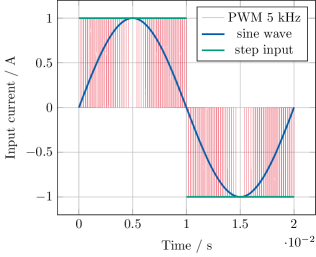
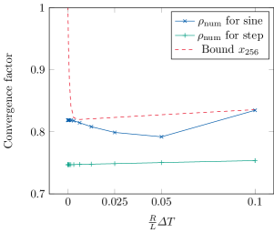
Figure 1: Left: PWM excitation (19) of $5$ kHz $(m=100)$ and two coarse inputs (20), (21). Right: convergence factor of the new periodic Parareal algorithm (5)-(6) with reduced coarse dynamics: sinusoidal waveform (20) and step function (21), together with our theoretical bound.

This figure also illustrates the following two choices for the coarse excitation:

$$\bar{f}_{\mathrm{sine}}(t) =\sin\left(\frac{2\pi}{T}t\right),\quad t\in[0,T],$$ (20)

$$\bar{f}_{\mathrm{step}}(t) =\begin{cases}1,\ &t\in[0,T/2],\\ -1,\ &t\in(T/2,T].\end{cases}$$ (21)

We note that the step function (21) is discontinuous only at $t=T/2$. This does not lead to any difficulties, since we use Backward Euler for the time discretization and we choose the discontinuity to be located exactly at a synchronization point.

The coarse propagator $\bar{\mathcal{G}}$ then solves an IVP for the equation $R^{-1}\phi^{\prime}(t)+L^{-1}\phi(t)=\bar{f}(t),\ t\in(0,T]$, where the RHS $\bar{f}$ is one of the functions in (20) or (21). We illustrate the estimate (17) by calculating the numerical convergence factor $\rho_{\mathrm{num}}:=\left(\|\mbox{\boldmath$e$}^{(K)}\|/\|\mbox{\boldmath$e$}^{(0)}\|\right)^{1/K}$ with the $l^{\infty}$-norm of the error $\mbox{\boldmath$e$}^{(k)}$ at iteration $k\in\{0,K\}$ defined as

$$\|\mbox{\boldmath$e$}^{(k)}\|=\max\limits_{0\leq n\leq N}|\phi(T_{n})-\Phi_{n}^{(k)}|.$$ (22)

Here $\phi$ denotes the time-periodic steady-state solution of (18) having the same accuracy as the fine propagator, and $\Phi_{n}^{(K)}$ is the solution obtained at the $K$th iteration when (5)-(6) converged up to a prescribed tolerance. The stability function used for $x_{l}$ in (17) in case of Backward Euler is $\mbox{$\mathcal{R}$}\left(\frac{R}{L}\Delta T\right)=\left(1+\frac{R}{L}\Delta T\right)^{-1}.$

On the right in Figure 1, we show the measured convergence factor of the new Parareal iteration (5)-(6) for the two choices of the coarse excitation (20) and (21). The fine step size is chosen to be $\delta T=T/2^{18}\sim 7.63^{-8}$, while the coarse step varies as $\Delta T=T/2^{p}$, $p=1,2,\dots,17$. We also show on the right in Figure 1 the value of $x_{256}$ to be the bound in (17). The graphs show that the theoretical estimate is indeed an upper bound for the numerical convergence factor for both coarse inputs (sine and step). However, one can observe that $x_{256}$ gives a sharper estimate in the case of the sinusoidal RHS (20), compared to the one defined in (21). We also noticed that the number of iterations required till convergence of (5)-(6) was the same (9 iterations on average for the values of $\Delta T$ considered) for both choices of the coarse input, while the initial error $\|\mbox{\boldmath$e$}^{(0)}\|$ was bigger with the step coarse input (21) than with the sinusoidal waveform (20). This led to a slightly smaller convergence factor in case of the step coarse input due to the definition of $\rho_{\mathrm{num}}$.

5 Numerical experiments for an induction machine

We now test the performance of our new periodic Parareal algorithm with reduced coarse dynamics for the simulation of a four-pole squirrel-cage induction motor, excited by a three-phase PWM voltage source switching at $20$ kHz. The model of this induction machine was introduced in Gyselinck_2001aa . We consider the no-load condition, when the motor operates with synchronous speed.

The spatial discretization of the two-dimensional cross-section of the machine with $n=4400$ degrees of freedom leads to a time-periodic problem represented by the system of differential-algebraic equations (DAEs)

$$\mathbf{M}\mathrm{d}_{t}\mathbf{u}(t)+\mathbf{K}\left(\mathbf{u}(t)\right)\mathbf{u}(t) =\mathbf{f}(t),\quad{t\in(0,T)},$$ (23)

$$\mathbf{u}(0) =\mathbf{u}(T),$$ (24)

with unknown $\mathbf{u}:[0,T]\to\mathbb{R}^{n},$ (singular) mass matrix $\mathbf{M}\in\mathbb{R}^{n\times n},$ nonlinear stiffness matrix $\mathbf{K}\left(\cdot\right):\mathbb{R}^{n}\to\mathbb{R}^{n\times n},$ and the $T$-periodic RHS $\mathbf{f}:[0,T]\to\mathbb{R}^{n},$ $T=0.02$ s. The three-phase PWM excitation of period $T$ in the stator under the no-load operation causes the $T$-periodic dynamics in $\mathbf{u}$ which allows the imposition of the periodic constraint (24). For more details regarding the mathematical model we refer to Kulchytska-Ruchka_2018ac . We would like to note that equation (23) is a DAE of index-$1,$ which in case of discretization with Backward Euler can be treated essentially like an ODE Schops_2018aa .

We now use our new periodic Parareal algorithm (5)-(6) to find the solution of (23)-(24). The fine propagator $\mathcal{F}$ is then applied to (23) with the original three-phase PWM excitation of $20$ kHz, discretized with the time step $\delta T=10^{-6}$ s. The coarse solver $\bar{\mathcal{G}}$ uses a three-phase sinusoidal voltage source with frequency $50$ Hz of the form (20), discretized with the time step $\Delta T=10^{-3}$ s. Phase $1$ of the PWM signal switching at $5$ kHz as well as the applied periodic coarse excitation on $[0,0.02]$ s are shown on the left in Figure 2.

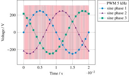
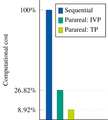
Figure 2: Left: PWM excitation (19) of $5$ kHz and three-phase sinusoidal voltage source of $50$ Hz, used as the coarse input in our new periodic Parareal algorithm (5)-(6). Right: comparison of the computational costs calculated in terms of the effective number of linear algebraic systems solved for different approaches to obtain the periodic steady-state solution of the induction machine model.

Both coarse and fine propagators solve the IVPs for (23) using Backward Euler, implemented within the GetDP library Geuzaine_2007aa . We used $N=20$ time subintervals for the simulation of the induction machine with our new periodic Parareal algorithm, which converged after $14$ iterations. Within these calculations $194\;038$ solutions of linearized systems of equations were performed effectively, i.e, when considering the fine solution cost only on one subinterval (due to parallelization) together with the sequential coarse solves.

On the other hand, a classical way to obtain the periodic steady-state solution is to apply a time integrator sequentially, starting from a zero initial value at $t=0$. This computation reached the steady state after $9$ periods, thereby requiring $2\;176\;179$ linear system solves. Alternatively, one could apply the Parareal algorithm with reduced coarse dynamics, introduced in Kulchytska-Ruchka_2018ac , to the IVP for (23) on $[0,9T]$. In this case the simulation needed effectively $583\;707$ sequential linear solutions due to parallelization. However, in practice one would not know the number of periods beforehand and one could not optimally distribute the time intervals. We visualize this data on the right in Figure 2. These results show that our new periodic Parareal algorithm (5)-(6) with reduced coarse dynamics directly delivers the periodic steady-state solution about $11$ times faster than the standard time integration, and $3$ times faster than the application of Parareal with the reduced dynamics to an IVP on $[0,9T]$.

6 Conclusions

We introduced a new periodic Parareal algorithm with reduced dynamics, which is able to efficiently handle quickly-switching discontinuous excitations in time-periodic problems. We investigated its convergence properties theoretically, and illustrated them via application to a linear RL-circuit example. We then tested the performance of our new periodic Parareal algorithm in the simulation of a two-dimensional model of a four-pole squirrel-cage induction machine, and a significant acceleration of convergence to the steady state was observed. In particular, with our new periodic Parareal algorithm with reduced dynamics it is possible to obtain the periodic solution $11$ times faster than when performing the classical time stepping.

References

- (1) Bermúdez, A., Domínguez, s., Gómez, D., Pilar, S.: Finite element approximation of nonlinear transient magnetic problems involving periodic potential drop excitations. Comput. Math. Appl. 65(8), 1200–1219 (2013)
- (2) Bose, B.K.: Power Electronics And Motor Drives. Academic Press, Burlington (2006)
- (3) Gander, M.J., Hairer, E.: Nonlinear convergence analysis for the Parareal algorithm. Springer (2008)
- (4) Gander, M.J., Jiang, Y.L., Song, B., Zhang, H.: Analysis of two parareal algorithms for time-periodic problems. SIAM J. Sci. Comput. 35(5), A2393–A2415 (2013). DOI 10.1137/130909172
- (5) Gander, M.J., Kulchytska-Ruchka, I., Niyonzima, I., Schöps, S.: A New Parareal Algorithm for Problems with Discontinuous Sources. ArXiv e-prints (2018)
- (6) Gander, M.J., Vandewalle, S.: Analysis of the Parareal time-parallel time-integration method. SIAM Journal on Scientific Computing 29(2), 556–578 (2007)
- (7) Geuzaine, C.: GetDP: a general finite-element solver for the de Rham complex. PAMM 7(1), 1010603–1010604 (2007). DOI 10.1002/pamm.200700750
- (8) Gyselinck, J., Vandevelde, L., Melkebeek, J.: Multi-slice FE modeling of electrical machines with skewed slots-the skew discretization error. IEEE Trans. Magn. 37(5), 3233–3237 (2001). DOI 10.1109/20.952584
- (9) Katagiri, H., Kawase, Y., Yamaguchi, T., Tsuji, T., Shibayama, Y.: Improvement of convergence characteristics for steady-state analysis of motors with simplified singularity decomposition-explicit error correction method. IEEE Trans. Magn. 47(5), 1458–1461 (2011)
- (10) Lions, J.L., Maday, Y., Turinici, G.: A parareal in time discretization of PDEs. Comptes Rendus de l’Académie des Sciences – Series I – Mathematics 332(7), 661–668 (2001). DOI 10.1016/S0764-4442(00)01793-6
- (11) Niyomsatian, K., Vanassche, P., Sabariego, R.V., Gyselinck, J.: Systematic control design for half-bridge converters with LCL output filters through virtual circuit similarity transformations. In: 2017 IEEE Energy Conversion Congress and Exposition (ECCE), pp. 2895–2902 (2017)
- (12) Schöps, S., Niyonzima, I., Clemens, M.: Parallel-in-time simulation of eddy current problems using parareal. IEEE Trans. Magn. 54(3) (2018). DOI 10.1109/TMAG.2017.276309