Shorten Spatial-spectral RNN with Parallel-GRU for Hyperspectral Image Classification

Abstract

Convolutional neural networks (CNNs) attained a good performance in hyperspectral sensing image (HSI) classification, but CNNs consider spectra as orderless vectors. Therefore, considering the spectra as sequences, recurrent neural networks (RNNs) have been applied in HSI classification, for RNNs is skilled at dealing with sequential data. However, for a long-sequence task, RNNs is difficult for training and not as effective as we expected. Besides, spatial contextual features are not considered in RNNs. In this study, we propose a Shorten Spatial-spectral RNN with Parallel-GRU (St-SS-pGRU) for HSI classification. A shorten RNN is more efficient and easier for training than band-by-band RNN. By combining converlusion layer, the St-SSpGRU model considers not only spectral but also spatial feature, which results in a better performance. An architecture named parallel-GRU is also proposed and applied in St-SS-pGRU. With this architecture, the model gets a better performance and is more robust.

I Introduction

Hyperspectral image (HSI) has attracted considerable attention in the remote sensing community and been widely used in various areas [1]. With the rich spectral information in HSI, different land cover categories can potentially be differentiated precisely.

In recent years, deep learning has been widely used in various fields, including HSI classification [2]. Convolutional neural networks (CNNs) and residual networks (ResNets) have obtained a successful result for HSI classification [3, 4]. Recurrent neural networks (RNNs) are also applied in HSI classification [5].

Because of the ability to extract the spatial contextual information, CNNs and ResNets can achieve a high accuracy in the classification task. However, CNNs and ResNets consider spectra as orderless vectors in $d$-dimensional feature space where $d$ represents the number of bands. However, spectra can be seen as orderly and continuing sequences in the spectral space. In other words, CNNs and ResNets ignore the continuity of spectra [5].

RNNs have proved effective in solving many challenging problems involving sequential data, such as Natural Language Processing (NLP) [6] and prediction of time series [7]. Considering the spectrum as a sequential sequence, the application of RNNs is reasonable as it can take full advantage of the high spectral resolution characteristics of HSI. However, for a long-sequence task, RNNs is not as effective as we expected. Long distance dependence, gradient vanish and overfitting are prone to occur [8]. Even if the long short-term memory network (LSTM) [9] is used to solve the long-distance dependence problem, RNNs is still hard for training and easily overfitting in a long-sequence task.

In previous work, 3D-CNN is applied in HSI classification and obtained a good behavior [10, 11]. For RNNs, Convolutional-LSTM (CLSTM) [12] also achieved a good performance in HSI classification [13]. 3D-CNNs and CLSTM consider both spatial contextual information and spectral continuity, which result in a high accuracy. Nevertheless, it takes a long time to train these two models.

In [5], LSTM and its variant, GRU [14], are applied in HIS classification, and it is proved that GRU has a better performance in HIS classification. To solve the problem that RNNs are easily over-fitting and difficult for training, [15] proposed band-group LSTM, which can effectively make training easier by reducing the number of timestep in LSTM.

In this study, a Shorten Spatial-spectral RNN with Parallel-GRU (St-SS-pGRU) is proposed. This study contributes to the literature in 2 major respects:

1)

A shorten RNN with GRU is applied in HIS classification. The model is more efficient and easier for training than band-by-band RNN. By combining converlusion layer, an advanced model Shorten Spatial-spectral RNN with GRU is proposed. The model considers not only spectral but also spatial feature, which leads to a better performance.

2)

An architecture named parallel-GRU is proposed and the model with this architecture has a better performance and is more robust.

The remainder of this paper is organized as follows. In the methodology section, firstly the structure of traditional RNN, LSTM and GRU are introduced and then the architecture of the proposed models are described. In the experimental section, the network setup, the experimental results, and the comparison of different models are provided. Finally, the conclusion section concludes the paper.

II Methodology

II-A Recurrent neural networks (RNN)

Different from Artificial neural network (ANN), RNN [9], a neural network with recurrent unit, has a better performance in solving many challenging problems involving sequential data analysis. The state of each time step of the recurrent unit is not only related to the input of the current step, but also related to the state of the previous step. Thus, the state of the preceding step can effectively influence the next step.

Given a sequence sample $\mathbf{x}={\begin{bmatrix}\mathbf{x}^{(1)},\mathbf{x}^{(2)},...,\mathbf{x}^{(m)}\end{bmatrix}}^{\top}$, in which $\mathbf{x}^{(t)}$ is the data at $t$th timestep. For the $t$th recurrent unit, its hidden state can be described as:

$$\mathbf{h}^{(t)}=\left\{\begin{matrix}\mathbf{h}^{(0)}&t=0\\ h(\mathbf{h}^{(t-1)},\mathbf{x}^{(t)})&t>0\end{matrix}\right.,$$ (1)

where $\mathbf{h}^{(0)}$ is the initial state of the recurrent unit, $h$ is a nonlinear function. Normally, $\mathbf{h}^{(0)}$ is set as a zero vector.

Optionally, in $t$th timestep, the recurrent unit may have an output $\mathbf{y}^{(t)}$. For some task, the RNN model will finally have an output vector $\mathbf{y}={\begin{bmatrix}\mathbf{y}^{(1)},\mathbf{y}^{(2)},...,\mathbf{y}^{(m)}\end{bmatrix}}^{\top}$, while for classification tasks, only one output is needed. Generally, The last output is adopted:

$$\mathbf{y}^{(t)}=y(\mathbf{h}^{(t)})$$ (2)

The recurrent unit in a traditional RNN is shown in Fig. 1. In the traditional RNN model, the update rule of the recurrent hidden state and output in Eq. (1) and (2) is usually implemented as follows:

$$h(\mathbf{h}^{(t-1)},\mathbf{x}^{(t)})=\varphi(\mathbf{W}_{h}\mathbf{x}^{(t)}+\mathbf{U}_{h}\mathbf{h}^{(t-1)}+\mathbf{b}_{h}),$$ (3)

$$y(\mathbf{h}^{(t)})=\mathbf{W}_{y}\mathbf{h}^{(t)}+\mathbf{b}_{y},$$ (4)

where $\mathbf{W}_{h}$, $\mathbf{U}_{h}$ and $\mathbf{W}_{y}$ are the weight matrices. $\mathbf{b}_{h}$ and $\mathbf{b}_{y}$ are the bias vectors, and $\varphi$ is an activation function, such as the sigmoid function or the hyperbolic tangent function.

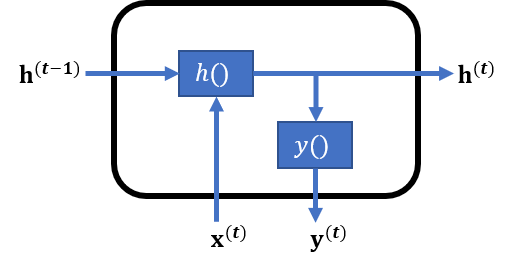
Figure 1: Graphic model of traditional recurrent unit.

II-B Long short-term memory (LSTM)

The traditional RNN has the problem of long-distance dependence [8]. The RNN has the capability to connect different timesteps related information. However, when the sequence is too long, the RNN becomes unable to connect related information as the distance increases, because the information losses when propagating through multi-time-step recurrent units.

By using long short-term memory (LSTM) [16], the problems have been solved. As Fig. 2 shows, LSTM contains a forget gate, an input gate and an output gate. ’Gate’ structure is actually a logistic regression model so that part of the information is filtered selectively, while the rest is reserved and passes through the gate. LSTM can simulate the process of forgetting and memory and calculate the probability of forgetting and memory, so information flow could be preserved in long-distance propagation. The structure of LSTM can be described as:

$$\mathbf{f}^{(t)}=\sigma(\mathbf{W}_{f}\mathbf{x}^{(t)}+\mathbf{U}_{f}\mathbf{h}^{(t-1)}+\mathbf{b}_{f}),$$ (5)

$$\mathbf{i}^{(t)}=\sigma(\mathbf{W}_{i}\mathbf{x}^{(t)}+\mathbf{U}_{i}\mathbf{h}^{(t-1)}+\mathbf{b}_{i}),$$ (6)

$$\mathbf{o}^{(t)}=\sigma(\mathbf{W}_{o}\mathbf{x}^{(t)}+\mathbf{U}_{o}\mathbf{h}^{(t-1)}+\mathbf{b}_{o}),$$ (7)

$$\tilde{\mathbf{c}}^{(t)}=tanh(\mathbf{W}_{c}\mathbf{x}^{(t)}+\mathbf{U}_{c}\mathbf{h}^{(t-1)}+\mathbf{b}_{c}),$$ (8)

$$\mathbf{c}^{(t)}=\mathbf{i}^{(t)}*\tilde{\mathbf{c}}^{(t)}+\mathbf{f}^{(t)}*\mathbf{c}^{(t-1)},$$ (9)

$$\mathbf{h}^{(t)}=\mathbf{o}^{(t)}*tanh(\mathbf{c}^{(t)}),$$ (10)

where Eq. (5), (6) and (7) represent forget gate, input gate and output gate. $\mathbf{W}_{f}$, $\mathbf{W}_{i}$, $\mathbf{W}_{o}$, $\mathbf{W}_{c}$, $\mathbf{U}_{f}$, $\mathbf{U}_{i}$, $\mathbf{U}_{o}$ and $\mathbf{U}_{c}$ are the weight matrices. $\mathbf{b}_{f}$, $\mathbf{b}_{i}$, $\mathbf{b}_{o}$ and $\mathbf{b}_{c}$ are the bias vectors. $\sigma$ refers to sigmoid function and tanh refers to the hyperbolic tangent function:

$$\sigma(x)=\frac{1}{1+e^{(}-x)},$$ (11)

$$tanh(x)=\frac{e^{x}-e^{(}-x)}{e^{x}+e^{(}-x)},$$ (12)

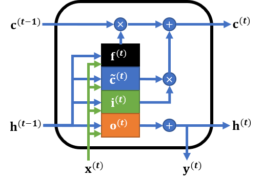
Figure 2: Graphic model of LSTM.

II-C Gated recurrent unit (GRU)

Over the years, there have been many variants of LSTM, but there is no evidence to show that there is not a superior variant. Any variant may have advantages in a particular problem [17].

GRU [14] is a variant of LSTM. With fewer parameters, it is much easier for training than LSTM, and usually achieves the same performance as LSTM in some tasks [18]. It is considered that using GRU in a HSI classification task is more appropriate than using LSTM [5].

The main difference between LSTM and GRU is that an update gate and a reset gate are adopted in GRU, instead of using a forget gate, an input gate and an output gate. The structure of the GRU is shown in Fig. 3, which can be defined as follows:

$$\mathbf{z}^{(t)}=\sigma(\mathbf{W}_{z}\mathbf{x}^{(t)}+\mathbf{U}_{z}\mathbf{h}^{(t-1)}+\mathbf{b}_{z}),$$ (13)

$$\mathbf{r}^{(t)}=\sigma(\mathbf{W}_{r}\mathbf{x}^{(t)}+\mathbf{U}_{r}\mathbf{h}^{(t-1)}+\mathbf{b}_{r}),$$ (14)

$$\tilde{\mathbf{h}}^{(t)}=tanh(\mathbf{W}_{h}\mathbf{x}^{(t)}+\mathbf{U}_{h}(\mathbf{r}^{(t)}*\mathbf{h}^{(t-1)})+\mathbf{b}_{h}),$$ (15)

$$\mathbf{h}^{(t)}=(1-\mathbf{z}^{(t)})\mathbf{h}^{(t-1)}+\mathbf{z}^{(t)}\tilde{\mathbf{h}}^{(t)},$$ (16)

where Eq. (13) and (14) represent update gate and reset gate. $\mathbf{W}_{z}$, $\mathbf{W}_{r}$, $\mathbf{W}_{h}$, $\mathbf{U}_{z}$, $\mathbf{U}_{r}$ and $\mathbf{U}_{h}$ are the weight matrices. $\mathbf{b}_{z}$, $\mathbf{b}_{r}$ and $\mathbf{b}_{h}$ are the bias vectors.

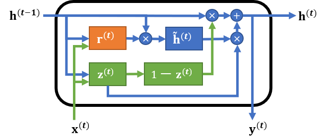
Figure 3: Graphic model of GRU.

II-D The proposed model

II-D1 Shorten Spatial-spectral RNN with GRU(St-SS-GRU)

A Shorten Spatial-spectral RNN with GRU (St-SS-GRU) model for HSI classification is shown in Fig. 4. For each pixel, a square subgraph composed of 5$\times$5 pixels centered on it is used as a training sample.

The first part of St-SS-GRU is actually a 3D-Convolutional layer but both the depth and stride of the kernels are 1. Three different convolution kernels (1×1, 3×3, 5×5) were used to convolve different bands. The output of this part is a sequence with the same length as the original input. The output sequence is a ’spectra’ with the spatial contextual feature. Every timestep of the sequence is a feature vector.

The second part is a Shorten RNN with GRU (St-GRU). The structure of St-GRU is shown in Fig. 5. The 1D converlusion layer before GRU is used to reduce the number of timesteps so that the network is easier for training.

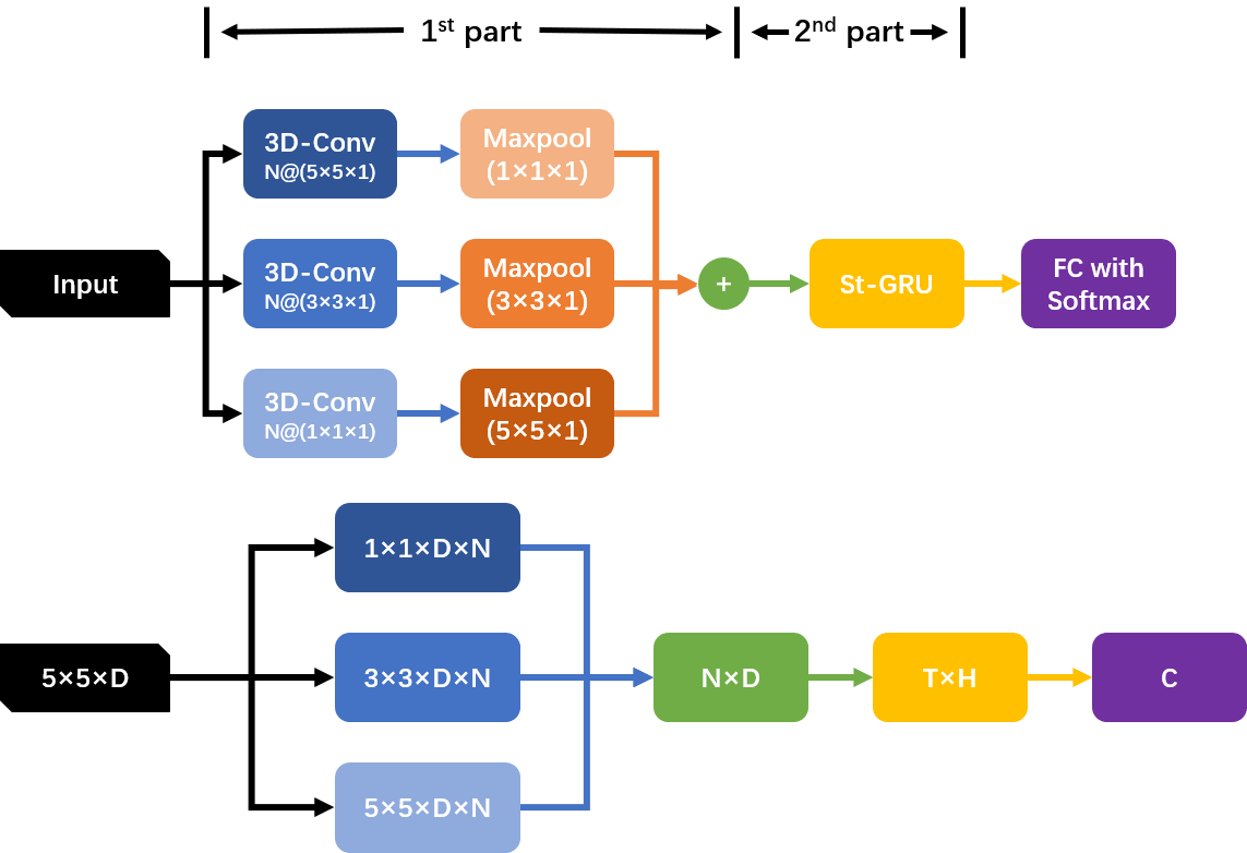
Figure 4: St-SS-GRU: (1) The first row shows a flowchart of the network. FC refers to fully connected layer and Conv refers to Convolutional layers. (2) The second row illustrates the shapes of input and output tensors of each layer and their connection. (3) N is the number of filters in the 3D-Convolutional layer, D is the number of bands in the input image, T is the number of GRU timestep, and H is the number of neurons in hidden layer in a GRU. For the Pavia University dataset, D=103, and in the experiment the hyperparameters are set as: N=16, T=5, H=128.

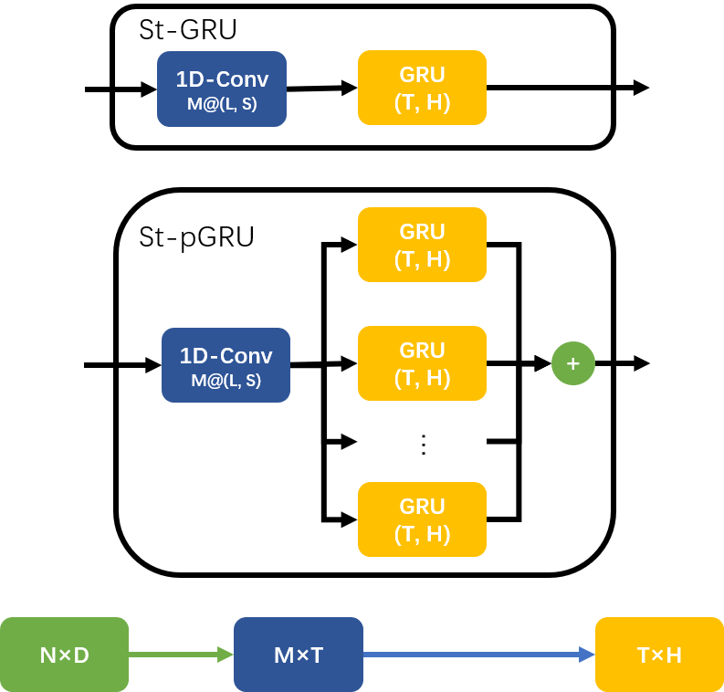
Figure 5: St-GRU and St-pGRU: (1) The first two rows show the architecture of St-GRU and St-pGRU, Conv refers to convolutional layers. (2) The third row illustrates the shapes of input and output tensors of each layer and their connection. (3) D is the number of bands in the input image, N is the dimension of the vector in each band of input, M is the number of filters in the 1D-Convolutional layer, T is the number of GRU timestep, and H is the number of neurons in hidden layer in a GRU. L and S, which are determined by T, refer to the size and stride of filters in the 1D-Convolutional layer. For the Pavia University dataset, D=103, and in the experiment the hyperparameter is set as: N=M=16, T=5, H=128.

II-D2 Parallel-GRU Architecture

In order to make the model more robust, a Parallel-GRU (pGRU) architecture is proposed. The architecture of Shorten Parallel-GRU (St-pGRU) is shown in Fig. 5. The architecture is actually a combination of several GRU units. The output of the architecture is the summation of every unit.

The Shorten Spatial-spectral RNN with parallel-GRU (St-SS-pGRU) is similar to St-SS-GRU, except that St-GRU is replaced by St-SS-pGRU.

III Experiment

III-A Data

In the experiment, two HSI datasets, including the Pavia University and Indian Pines, are used to evaluate the performance of the proposed model.

The Pavia University dataset was acquired by the Reflective Optics System Imaging Spectrometer(ROSIS) sensor over Pavia, northern Italy in 2001. The corrected data, with a spatial resolution of 1.3 m per pixel, contains 103 spectral bands ranging from 0.43 to 0.86 $\mu m$. The image, with 610$\times$340 pixels, is differentiated into 9 ground truth classes. Table I provides information about all classes of the dataset with their corresponding training and test sample.

The Indian Pines dataset was acquired by the TAirborne Visible/Infrared Imaging Spectrometer (AVIRIS) sensor over the Indian Pines test site in north-western Indiana in 1992. The corrected data with a moderate spatial resolution of 20m contains 200 spectral bands ranging from 0.4 to 2.5 $\mu m$. The image consists of 145$\times$145 pixels, which are differentiated into 16 ground truth classes. Table II provides information about all classes of the dataset with their corresponding training and test sample.

TABLE I: Number of Training and Test Samples Used in the Pavia University Dataset

No.	Class Name	Training Samples	Test Samples
1	Asphalt	548	6083
2	Meadows	540	18109
3	Gravel	392	1707
4	Trees	542	2522
5	Metal sheet	256	1089
6	Bare Soil	532	4497
7	Bitumen	375	955
8	Bricks	514	3168
9	Shadows	231	716
	TOTAL	3921	38846

TABLE II: Number of Training and Test Samples Used in the Indian Pines Dataset

No.	Class Name	Training Samples	Test Samples
1	Alfalfa	30	16
2	Corn-notill	150	1278
3	Corn-min	150	680
4	Corn	100	137
5	Grass-pasture	150	333
6	Grass-trees	150	580
7	Grass-pasture-mowed	20	8
8	Hay-windrowed	150	328
9	Oats	15	5
10	Soybean-notill	150	822
11	Soybean-mintill	150	2305
12	Soybean-clean	150	443
13	Wheat	150	55
14	Woods	150	1115
15	Building-grass-trees	50	336
16	Stone-stell-towers	50	43
	TOTAL	1765	8484

III-B Result

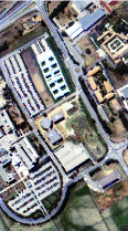
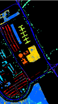
(a) False color map	(b) Ground truth	(c) GRU(87.79%)
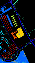
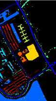
(e) St-GRU(92.38%)	(f) St-SS-GRU(98.04%)	(g) St-SS-pGRU(99.01%)

Figure 6: The classification maps of the Pavia University dataset.

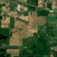
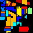
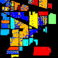
(a) False color map	(b) Ground truth	(c) GRU(77.07%)
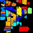
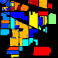
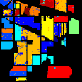
(e) St-GRU(80.50%)	(f) St-SS-GRU(86.28%)	(g) St-SS-pGRU(89.61%)

Figure 7: The classification maps of the Indian Pines dataset.

Table III and IV list the results obtained by the experiment, and Fig. 6 and 7 show the classification maps on the Pavia University dataset and the Indian Pines dataset. Note that the accuracies list in Table III and IV are overall accuracies (OA) along with the standard deviation, from 10 independent runs on each dataset. The experiment is implemented with an Intel i7-7700K 4.20GHz processor with 16GB of RAM and an NVIDIA GTX1050Ti graphic card under Python3.6 with tensorflow1.8.0.

First of all, for all the datasets, GRU outperforms LSTM. In addition, it is observed that LSTM is difficult to converge in the experiment, while GRU is not. Thus, it is reasonable to indicate that GRU is a better choice for a HSI classification task.

Furthermore, it is apparent that St-GRU increases the accuracy significantly by 5.33% and 3.52% in the Pavia University dataset and the Indian Pines correspondingly. With converlusion layers, St-SS-GRU has a better than St-GRU. The accuracy of St-SS-GRU is 4.55% and 6.63% higher than that in St-GRU. After parallel-GRU is adopted, the model gains the best performance in this experiment. The accuracy of St-SS-pGRU is 1.64% and 3.19% higher than St-SS-GRU. What is more, the standard deviation of St-SS-pGRU is smaller than other models, which indicate that St-SS-pGRU is more robust.

Comparing the processing time of different methods, st-GRU is significantly faster in training than band-by-band GRU. St-SS-GRU and St-SS-pGRU are as slow as LSTM and GRU in training, but they have higher accuracies than LSTM and GRU.

TABLE III: Classification Accuracies and Training Time for the Pavia University Dataset

Model	Overall accuracy	Training Time (s)
LSTM	84.68$\pm$1.40%	434.22
GRU	86.92$\pm$1.29%	232.15
St-GRU	92.25$\pm$0.78%	7.31*
St-SS-GRU	96.80$\pm$0.37%	104.56
St-SS-pGRU	98.44$\pm$0.26%*	128.91
* The best performance in each column is shown in bold.

TABLE IV: Classification Accuracies and Training Time for the Indian Pines Dataset

Model	Overall accuracy	Training Time (s)
LSTM	71.65$\pm$1.05%	838.85
GRU	77.01$\pm$1.82%	442.67
St-GRU	80.53$\pm$0.90%	7.63*
St-SS-GRU	87.16$\pm$1.06%	287.54
St-SS-pGRU	90.35$\pm$0.86%*	300.90
* The best performance in each column is shown in bold.

IV Conclusion

In the study, a St-SS-pGRU model is proposed for HSI classification. What is more, an architecture named parallel-GRU is proposed to promote the performance and robustness. Then an experiment is conducted to compare the performance of different models. From the experiment, it is confirmed that GRU performs better than LSTM in HSI classification task. Moreover, it is apparent that the proposed models are a lot more accurate, more robust and faster than the traditional GRU network. Specifically, St-GRU effectively reduced the training time and promoted the accuracy. St-SS-GRU needs more time for training but gains a better performance than St-GRU. The proposed architecture parallel-GRU also provided a satisfactory result in the experiment.

References

- [1] José M Bioucas-Dias, Antonio Plaza, Gustavo Camps-Valls, Paul Scheunders, Nasser Nasrabadi, and Jocelyn Chanussot. Hyperspectral remote sensing data analysis and future challenges. IEEE Geoscience and remote sensing magazine, 1(2):6–36, 2013.
- [2] Xiao Xiang Zhu, Devis Tuia, Lichao Mou, Gui-Song Xia, Liangpei Zhang, Feng Xu, and Friedrich Fraundorfer. Deep learning in remote sensing: A comprehensive review and list of resources. IEEE Geoscience and Remote Sensing Magazine, 5(4):8–36, 2017.
- [3] Hyungtae Lee and Heesung Kwon. Going deeper with contextual cnn for hyperspectral image classification. IEEE Transactions on Image Processing, 26(10):4843–4855, 2017.
- [4] Zilong Zhong, Jonathan Li, Lingfei Ma, Han Jiang, and He Zhao. Deep residual networks for hyperspectral image classification. Institute of Electrical and Electronics Engineers, 2017.
- [5] Lichao Mou, Pedram Ghamisi, and Xiao Xiang Zhu. Deep recurrent neural networks for hyperspectral image classification. IEEE Transactions on Geoscience and Remote Sensing, 55(7):3639–3655, 2017.
- [6] Martin Sundermeyer, Hermann Ney, and Ralf Schlüter. From feedforward to recurrent lstm neural networks for language modeling. IEEE Transactions on Audio, Speech, and Language Processing, 23(3):517–529, 2015.
- [7] Felix A Gers, Douglas Eck, and Jürgen Schmidhuber. Applying lstm to time series predictable through time-window approaches. In Neural Nets WIRN Vietri-01, pages 193–200. Springer, 2002.
- [8] Yoshua Bengio, Patrice Simard, and Paolo Frasconi. Learning long-term dependencies with gradient descent is difficult. IEEE transactions on neural networks, 5(2):157–166, 1994.
- [9] Ronald J Williams and David Zipser. A learning algorithm for continually running fully recurrent neural networks. Neural computation, 1(2):270–280, 1989.
- [10] Ying Li, Haokui Zhang, and Qiang Shen. Spectral–spatial classification of hyperspectral imagery with 3d convolutional neural network. Remote Sensing, 9(1):67, 2017.
- [11] Zilong Zhong, Jonathan Li, Zhiming Luo, and Michael Chapman. Spectral–spatial residual network for hyperspectral image classification: A 3-d deep learning framework. IEEE Transactions on Geoscience and Remote Sensing, 56(2):847–858, 2018.
- [12] SHI Xingjian, Zhourong Chen, Hao Wang, Dit-Yan Yeung, Wai-Kin Wong, and Wang-chun Woo. Convolutional lstm network: A machine learning approach for precipitation nowcasting. In Advances in neural information processing systems, pages 802–810, 2015.
- [13] Qingshan Liu, Feng Zhou, Renlong Hang, and Xiaotong Yuan. Bidirectional-convolutional lstm based spectral-spatial feature learning for hyperspectral image classification. Remote Sensing, 9(12):1330, 2017.
- [14] Kaisheng Yao, Trevor Cohn, Katerina Vylomova, Kevin Duh, and Chris Dyer. Depth-gated recurrent neural networks. arXiv preprint arXiv:1508.03790, 2015.
- [15] Yonghao Xu, Bo Du, Liangpei Zhang, and Fan Zhang. A band grouping based lstm algorithm for hyperspectral image classification. In CCF Chinese Conference on Computer Vision, pages 421–432. Springer, 2017.
- [16] Sepp Hochreiter and Jürgen Schmidhuber. Long short-term memory. Neural computation, 9(8):1735–1780, 1997.
- [17] Klaus Greff, Rupesh K Srivastava, Jan Koutník, Bas R Steunebrink, and Jürgen Schmidhuber. Lstm: A search space odyssey. IEEE transactions on neural networks and learning systems, 28(10):2222–2232, 2017.
- [18] Rafal Jozefowicz, Wojciech Zaremba, and Ilya Sutskever. An empirical exploration of recurrent network architectures. In International Conference on Machine Learning, pages 2342–2350, 2015.