Adaptive Eigenspace Segmentation

Abstract

Image segmentation is an inherently ill-posed problem and thus requires regularization in order to limit the search space to reasonable solutions. A majority of segmentation methods integrates these regularization terms in one way or the other in an energy functional using a balancing term. The tuning of this parameter that either favours more the regularization or the data conformity is critical and, unfortunately, the success of the optimization process strongly depends on it. Often the optimal settings change from image to image.

In this paper we propose a novel general framework based on an adaptive eigenspace that was first proposed for solving inverse problems. The resulting method proves accurate and yields robust results, without the need for optimization techniques or being sensitive to the parameter choice. In fact, the method solves a symmetric positive definite sparse system and hence, uses only a fraction of the computational cost. The method is very versatile and does not need parameter-tuning, when segmenting objects from any kind of an image or when segmenting different organs. As the adaptive eigenspace is determined directly from the image to segment, the approach also does not need a tedious training phase.
Keywords: Adaptive eigenspace, image segmentation, image processing, noise removal.

1 Introduction

Segmentation is a basic image processing technique that has spurred widespread interest during the last decades. Many of the proposed approaches use some form of regularization and often employ an iterative scheme. Regularization is recommended as it limits the result space to “meaningful” solutions.

Image segmentation is the process in which an algorithm divides a digital image into groups of connected pixels. The idea is to split the image domain into non-intersecting segments and that can subsequently be analyzed to extract higher-level information from the image. Segmentation of images has been an area of active research over more than 45 years now pavlidis1972segmentation and yet, finding a robust algorithm, which is able to segment different types of images without intensive parameter tuning or training is still a challenge. Furthermore, measurement noise and speckle, as seen in ultrasound or Optical Coherence Tomography (OCT) images, still pose a largely unsolved challenge. Many techniques were proposed over the years, see Angenent2006 for a concise overview, including very basic ones, such as thresholding, region growing or watershed, see for example adams1994seeded , fan2001automatic and shafarenko1997automatic . The idea behind region growing, for example, is to start in some seed points and to test if the neighboring pixels should be part of their segment. Those methods are very intuitive, but are not robust under noise.

In recent years, segmentation using deep learning and neural networks has become very popular and many papers were written and are still written on this topic, for example schmidhuber2015deep , litjens2017survey and andermatt2016multi . In contrast to the above mentioned methods, where the information is taken from the image to be segmented, in deep learning, the method tries to automatically learn the segmentation through a large dataset-collection of sample images and their segmentation’s correct labelling.

Besides the basic ad hoc segmentation approaches described above, a family of more principled segmentation approaches form the energy based techniques. This family includes techniques such as active contours, also known as snakes, see kass1988snakes and its various extensions cohen1991active ; Kichenassamy1996 ; caselles1997geodesic ; xu19972d ; bresson2007fast . In this method, a snake is a spline, which can be deformed to minimize the energy functional. The snake is influenced by constraints, called external and internal forces that deform it to match the contours of an object. Some of these energies force the snake to the contour of the image while others regularize the resulting contour to a “reasonable” result. Besides the snakes, other energy based techniques became popular such as the level-sets Chan2001 or the graph-cut BOYKOV2001 approaches. All these techniques represent different ways of solving an energy term which is similar for all of them. In fact they all try to minimize a positive cost functional $E$, where $I$ is the image to segment and $u$ the segmentation result

$$E[u;I]=F[u;I]+\eta\mathcal{R}[u]\,.$$ (1)

The energy $E$ is composed of two components, namely the fidelity term $F$ that forces the segmentation to match the source image as close as possible and the regularization term $\mathcal{R}$ ensures that the resulting segmentation is reasonable. The balancing term $\eta$ is common to these methods and is a parameter that needs careful tuning to each and every application separately as it balances the trade-off between closeness of the solution to the image and the regularization term. Depending on the application one may choose different kinds of penalty functionals $\mathcal{R}$ for regularization, including the common $L^{2}$-norm, the penalized TV-regularization, the Sobolev $H^{1}$-penalty functional, the Lorentzian penalty functional Tikhonov:1943:SIP ; Gene:1999:TRT ; Engl:1996:RIP .

The adaptive eigenspace (AE), initially introduced in deBuhan:2009:SRP and later in deBuhan:2013:AIM and in de2017numerical which is strongly related to gilboa2016nonlinear , was used in Grote:2016:AEI and in grote2017adaptive as a new regularization method, where the AE of the penalized TV-gradient was used to regularize an inverse medium problem. Instead of adding a penalty functional $\mathcal{R}$ to the minimization problem, we build the parameter from the eigenfunctions of the TV-regularization gradient drastically simplifying the optimization of the energy functional. The method was able to reduce dramatically the number of variables and to achieve very accurate solutions in smaller computational cost. In Nahum:2016:AEI , several eigenspaces from different regularization terms are introduced, one of those was the adaptive eigenspace of the Lorentzian regularization. In gilboa2016nonlinear , the nonlinear spectral representation is introduced. There, eigenfunctions of the TV-regularization and other convex functionals are used for image decomposition and denoising. The idea of segmenting images using eigenfunctions is also introduced in 7433409 , where eigenfunctions of an anisotropic diffusion operator were used successfully for image segmentation.

In this paper, we propose a general and versatile framework using the adaptive eigenspace of the non-convex Lorentzian penalty functional for segmentation. Instead of optimizing over the energy functional $E$, we compute the eigenfunctions of the gradient of the regularization term $\mathcal{R}$ and find the segmentation there. Here, we show how this approach can segment useful information with very low computational cost. As shown in Nahum:2016:AEI , the method does not need any parameter tuning, when recovering different media, the same applies for image segmentation. Using the AE for segmentation yields a fast, sparse and reliable method, which is very robust under noise or speckle. As the approach has no parameters there is no need for parameter-tuning such as balancing the term $\eta$ from (1) and is thus inherently insensitive to parameter tuning. Lastly, we show that the proposed novel segmentation approach can also be applied for noise reduction by segmenting the noise out (rather than filtering the noise).

This paper is organized in four parts. In Section 2, we show how to derive the AE of the Lorentzian. In Section 3 properties of the AE are introduced. In Section 4, we show mathematical evidence of the robustness and usefulness of the AE, using examples in one or two space dimensions. At last, in Section 5 we show some numerical results that underpin the efficiency and suitability of the AE to segment images, remove noise and combinations thereof.

2 Image Segmentation and Regularization

In image segmentation one uses, usually, a minimization problem of a positive energy functional $E$ to extract wanted information out of an image. For a given image $I$ and set of admissible parameters $U_{ad}$, one solves

$$u^{*}=\operatorname*{argmin}\limits_{u\in U_{ad}}\left\{F(u,I)+\eta\mathcal{R}(u)\right\}\,,$$ (2)

where $F$ is the fidelity term and $\mathcal{R}$ is a regularization functional, which provides any additional knowledge on the wished segmentation and tackles ill-posedness of the optimization problem. The parameter $\eta$ balances between those functionals.

For the regularization, one can choose different penalty functionals $\mathcal{R}(u)$: the standard Tikhonov Tikhonov:1943:SIP ; Vogel:2002:CMIP ; Gene:1999:TRT ; Engl:1996:RIP $L^{2}$-penalty functional

$$\mathcal{R}_{L^{2}}(u)=\frac{1}{2}\|u\|^{2}_{L^{2}}\,,$$ (3)

or the Sobolev $H^{1}$-penalty functional

$$\mathcal{R}_{\nabla u}(u)=\frac{1}{2}\int_{\Omega}\sum_{i=1}^{d}\left(\dfrac{\partial u}{\partial x_{i}}\right)^{2}\,dx\,,$$ (4)

which penalizes strong variation in the solution and leads to smooth results.

A popular penalty functional penalizes the Total Variation (TV) Vogel:1996:IMTV , and was originally introduced for noise removal in image processing Rudin:1992:NTV . While preserving important detail, regularizing images using the penalized TV, removed unwanted noise. It uses the $L^{1}$ norm and is given by

$$R_{TV}(u)=\frac{1}{2}\int_{\Omega}\sqrt{|\nabla u|^{2}+\varepsilon^{2}}\,dx\,,\quad\varepsilon\neq 0\,.$$ (5)

An important penalty functional from a group of non-convex regularization terms is the Lorentzian penalty term

$$R_{Lorentz}(u)=\frac{1}{2}\int_{\Omega}\dfrac{\gamma|\nabla u|^{2}}{1+\gamma|\nabla u|^{2}}\,dx\,,\quad\gamma>0\,.$$ (6)

It penalizes strong variations in the solution and contains an extra parameter $\gamma$ to allow discontinuities.

In contrast, when segmenting an image with the proposed adaptive eigenspace we do not optimize (2) but only have to compute the image’s eigenfunctions of the gradient of the regularization term $\mathcal{R}$. This approach has proved itself as very accurate and reliable in the inverse medium problems in Grote:2016:AEI . There, a severely ill-posed problem was solved and regularized using the adaptive eigenspace of the TV-regularization gradient with much success.

Unlike the inverse medium problem, here, the image to be segmented is known and we may use the image itself to build the adaptive eigenspace. Hence, we can use an AE of non-convex penalty terms, which may be more sensitive to changes in the gradient of the image. In Nahum:2016:AEI and in grote2017adaptive , several eigenspaces of different regularization terms are introduced, one of those was the adaptive eigenspace of the Lorentzian regularization. Here, we may use this regularization without intensifying the ill-posedness or non-convexity of the problem.

This results in an image-processing approach, which is not sensitive to a parameter choice and there is no need to change parameters when segmenting different kinds of images, including photos or medical images.

3 Principle of the Adaptive Eigenspace (AE)

The main purpose of image segmentation using the AE lies on the parametrization of the image $I$. Standard techniques use regularization methods and iterative methods on the image. Following Grote:2016:AEI , we propose to use the adaptive eigenspace as regularization. There, the parameter is unknown and we use the AE of the TV-regularization as regularization. Here, as the image $I$ is known, we follow Nahum:2016:AEI and derive the adaptive eigenspace of the Lorentzian regularization. For an image $I$ the Lorentzian regularization-functional is given by

$$R_{Lorentz}(I)=\frac{1}{2}\int_{\Omega}\dfrac{\gamma|\nabla I(x)|^{2}}{1+\gamma|\nabla I(x)|^{2}}\,dx\,,\quad\gamma>0\,.$$ (7)

Next, we compute the gradient of (7)

$$\nabla_{u}\mathcal{R}_{Lorentz}(I)=-\nabla\cdot\left(\dfrac{\gamma\nabla I(x)}{\left(1+\gamma|\nabla I(x)|^{2}\right)^{2}}\right)\,,\quad\gamma>0\,.$$ (8)

Following Nahum:2016:AEI , we build an adaptive eigenspace from (8), this means that we take the gradient from (8), substitute $I(x)$ into $\phi(x)$ only where $I(x)$ does not appear in an absolute value. Then, we impose Dirichlet boundary conditions and get the following eigenspace problem

$$\left\{\begin{array}[]{rclll}-\nabla\cdot\left(\dfrac{\gamma\nabla\phi_{m}(x)}{{\left(1+\gamma|\nabla I(x)|^{2}\right)^{2}}}\right)&=&\lambda_{m}\phi_{m}(x),&&\forall\,x\in\Omega,\\[1.99997pt] \phi_{m}(x)&=&0,&&\forall\,x\in\Gamma\,.\end{array}\right.$$ (9)

Now, we can expand $I(x)$ as

$$I\ =\ I_{0}(x)\ +\ \sum_{m\geq 1}\beta_{m}\phi_{m}(x),$$ (10)

where $I_{0}\in H^{1}(\Omega)$ is a prolongation of $c^{2}_{|\Gamma}\in H^{\frac{1}{2}}(\Gamma)$ and the functions $\phi_{m}\in H_{0}^{1}(\Omega)$ form a Hilbertian basis to parametrize $I-I_{0}$. The prologation $I_{0}$ is the eigenfunction corresponding to $\lambda=0$, which holds the same boundary data as $I$, namely

$$\left\{\begin{array}[]{rclll}-\nabla\cdot\left(\dfrac{\gamma\nabla I_{0}(x)}{{\left(1+\gamma|\nabla I(x)|^{2}\right)^{2}}}\right)&=&0,&&\forall\,x\in\Omega,\\[1.99997pt] I_{0}(x)&=&I(x),&&\forall\,x\in\Gamma.\end{array}\right.$$ (11)

4 Properties of the Adaptive Eigenspace Basis

4.1 One-dimensional case

In (10), we have used the basis of eigenfunctions $\{\phi_{m}\}_{m\geq 1}$ defined by (9) together with $I_{0}$ defined by (11). In this section, for a given image $I(x)$, we provide some analytical and numerical evidence which underpins the basis choice for segmentation of images with or without noise. Similar examinations for proving the usefulness of the methods were made for the penalized TV-regularization eigenspace in grote2017adaptive and for the spectral TV in gilboa2016nonlinear .

We can approximate an image $I$ in the eigenspace $\{\phi_{1},\phi_{2},\,\ldots,\,\phi_{K}\}$, where all $\phi_{m}(x)$ satisfy (12) in one space dimension:

$$\left\{\begin{array}[]{c}-\dfrac{d}{dx}\left(\mu(x)\dfrac{d}{dx}\phi_{m}(x)\right)=\lambda_{m}\phi_{m}(x)\qquad\forall\,x\in[a,b],\\[1.99997pt] \phi_{m}(a)=0\,,\quad\phi_{m}(b)=0,\end{array}\right.$$ (12)

where

$$\mu(x)=\dfrac{\gamma}{(|1+\gamma I^{\prime}(x)^{2})^{2}}\,,\quad\forall x\in[a,b].$$ (13)

The behavior of $\phi_{m}(x)$ strongly depends on the magnitude of $I^{\prime}(x)$.

If $|I^{\prime}(x)|\simeq C>\frac{1}{\sqrt{\gamma}}$ in some part of $\Omega,$ $\phi_{m}(x)$ behaves like $\phi_{m}(x)\simeq A\sin(C^{2}\sqrt{\lambda_{m}}\,x)+B\cos(C^{2}\sqrt{\lambda_{m}}\,x)$. However, if $I$ is constant in some part of $\Omega$, $|I^{\prime}(x)|=0$, then $\mu=\gamma$ there, and $\phi_{m}$ behaves like $\phi_{m}(x)\simeq A_{m}\sin(\sqrt{\frac{1}{\gamma}\lambda_{m}}\,x)+B_{m}\cos(\sqrt{\frac{1}{\gamma}\lambda_{m}}\,x)$. For large enough $\gamma$, $\phi_{m}(x)$ has very slow variation and remains constant.

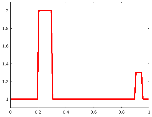
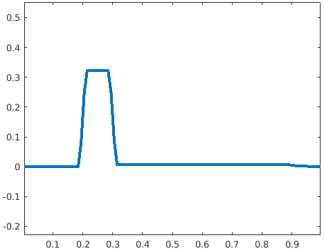
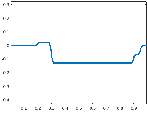
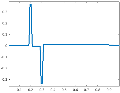
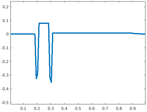
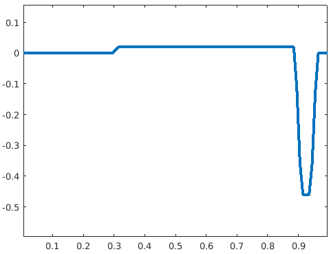
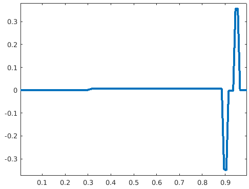
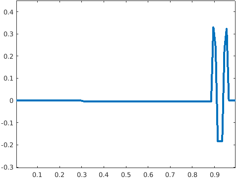
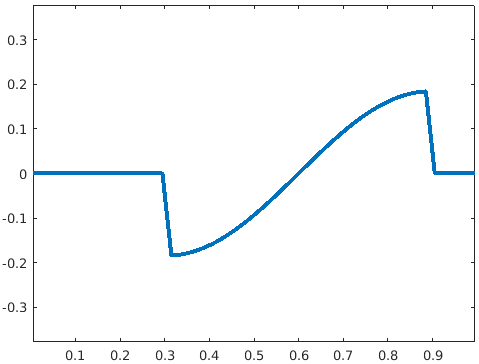
Figure 1: One-dimensional case. The true profile $I$ (top), together with the first eight eigenfunctions from (12) with $\gamma=\max(|I^{\prime}|)$.

To illustrate this behavior, we now consider the profile $I(x)$ containing two one-dimensional objects, as shown on the top of Fig. 1, note that $I^{\prime}(x)\neq 0$ for $0.19\leq x\leq 0.2$, $0.29\leq x\leq 0.3$, $0.89\leq x\leq 0.9$ and $0.95\leq x\leq 0.96$ and $I^{\prime}(x)=0$, otherwise. In Fig. 1, we present $I(x)$ together with some of its eigenfunctions from problem (12). We can see that $\phi_{1}(x)$ coincides to the first object in $I(x)$ and $\phi_{5}(x)$ to the second object in $I(x)$ (up to a constant). Actually, all the eigenfunctions, including those seen in Fig. 1, can be described as

$$\phi_{m}(x)\simeq\begin{cases}A_{m,1}\sin(\frac{1}{\sqrt{\gamma}}\sqrt{\lambda_{m}}\,x)+B_{m,1}\cos(\frac{1}{\sqrt{\gamma}}\sqrt{\lambda_{m}}\,x),&x\in[0.0,0.19),\\ A_{m,2}\sin(10^{4}\sqrt{\lambda_{m}}\,x)+B_{m,2}\cos(10^{4}\sqrt{\lambda_{m}}\,x),&x\in[0.19,0.2),\\ A_{m,3}\sin(\frac{1}{\sqrt{\gamma}}\sqrt{\lambda_{m}}\,x)+B_{m,3}\cos(\frac{1}{\sqrt{\gamma}}\sqrt{\lambda_{m}}\,x),&x\in[0.2,0.3),\\ A_{m,4}\sin(10^{4}\sqrt{\lambda_{m}}\,x)+B_{m,4}\cos(10^{4}\sqrt{\lambda_{m}}\,x),&x\in[0.3,0.31),\\ A_{m,5}\sin(\frac{1}{\sqrt{\gamma}}\sqrt{\lambda_{m}}\,x)+B_{m,5}\cos(\frac{1}{\sqrt{\gamma}}\sqrt{\lambda_{m}}\,x),&x\in[0.31,0.89)\\ A_{m,6}\sin(30^{2}\sqrt{\lambda_{m}}\,x)+B_{m,6}\cos(30^{2}\sqrt{\lambda_{m}}\,x),&x\in[0.89,0.9]\\ A_{m,7}\sin(\frac{1}{\sqrt{\gamma}}\sqrt{\lambda_{m}}\,x)+B_{m,7}\cos(\frac{1}{\sqrt{\gamma}}\sqrt{\lambda_{m}}\,x),&x\in[0.9,0.95)\\ A_{m,8}\sin(30^{2}\sqrt{\lambda_{m}}\,x)+B_{m,8}\cos(30^{2}\sqrt{\lambda_{m}}\,x),&x\in[0.95,0.96)\\ A_{m,9}\sin(\frac{1}{\sqrt{\gamma}}\sqrt{\lambda_{m}}\,x)+B_{m,9}\cos(\frac{1}{\sqrt{\gamma}}\sqrt{\lambda_{m}}\,x),&x\in[0.96,1].\end{cases}$$ (14)

For every interval, $\phi_{m}(x)$ has a different frequency, which is defined by the expression $C^{2}\sqrt{\lambda_{m}}$. For example, for each eigenfunction $\phi_{m}(x)$, the frequency in the subinterval $[0.3,0.31]$ is $\left(\frac{10}{3}\right)^{2}$ times higher than the frequency in the subinterval $[0.95,0.96)$ due to the strong dependency of $\mu$ from (13) in $I^{\prime}$ for $I^{\prime}\neq 0$ (it appears in high potency in the divisor of $\mu$). In the subintervals $[0.0,0.19),[0.2,0.3),[0.31,0.89),[0.9,0.95)$ and $[0.96,1)$, the frequency depends strongly on $\gamma$ which is chosen as $\gamma=\max(|I^{\prime}(x)|$. While $\frac{1}{\sqrt{\gamma}}\sqrt{\lambda_{m}}$ is very small, the eigenfunction $\phi_{m}(x)$ oscillates very slowly in this subinterval and thus behaves as a constant. As $\lambda_{m}$ increases, the frequency $\frac{1}{\sqrt{\gamma}}\sqrt{\lambda_{m}}$ increases as well and oscillations appear (see $\phi_{7}$ in Fig. 1, bottom right). Clearly, for high enough $\gamma$, more eigenfunctions $\phi_{m}(x)$ essentially behave as constants on this subinterval.

Finally, we consider $I$, shown in the top of Fig. 1, with $20\%$ of added noise such that

$$I_{noise}=I\left(1+\delta\,\xi\right)\,$$

where $\xi$ is uniformly distributed random number in the interval $(0,1)$ and $\delta=0.2$ represents the noise level. Since $\mu$ is strongly dependent in $I^{\prime}$, for $I^{\prime}\neq 0$, the first eigenfunction will essentially extract the objects from the added noise. The image $I_{noise}$ with $20\%$ of added noise is shown in Fig 2, together with the first eigenfunction $\phi_{1}$ and the fifth eigenfunction $\phi_{5}$ obtained from (12) using $I_{noise}$. Again, we observe that two of the eigenfunctions captures the elements appears in $I_{noise}$, this is up to a small perturbation, as can be seen in both eigenfunctions.

Remark 1.

although the eigenfunctions are not strictly segmentations as the are not binary labels, one can simply threshold them to yield binary segmentations.

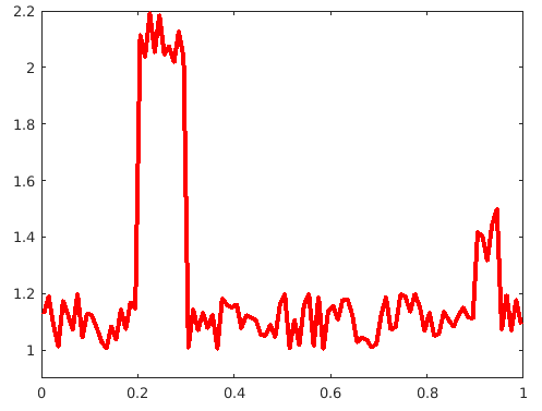
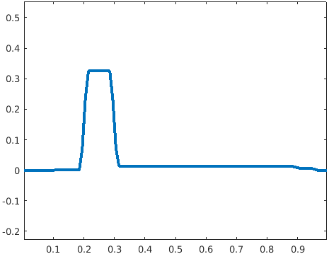
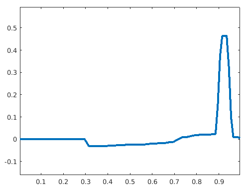
Figure 2: One-dimensional case. The noised image $I_{noise}$ (left) and the first and fifth eigenfunctions from (12) $\phi_{1}$ (center) and $\phi_{5}$ (right).

4.2 Two-dimensional case

To illustrate the remarkable approximation properties of the AE basis in two space dimensions, we now consider the image $I(x)$, $x=(x_{1},x_{2})$, shown in Fig. 3 (top, left). Assume we want to separate the different objects appearing in the image. We compute the first five eigenfunctions using (9) with $I(x)$ as input. Here, as in all examples in this paper, we take $\gamma=\max\left|\nabla I(x)\right|$. These results illustrate the remarkable properties of using the AE for segmentation. We are able to extract from the image, the stapler, the sharpener, the sellotape, the lid of the glue and the position of the slogan of the glue company.

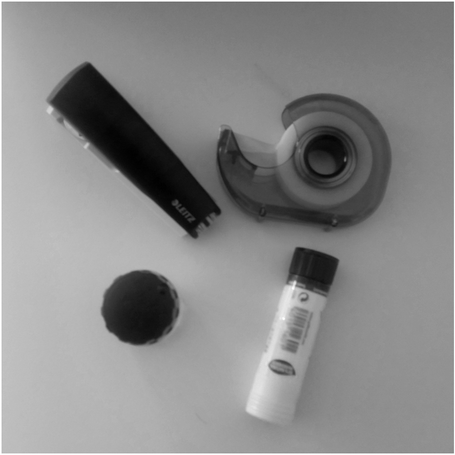
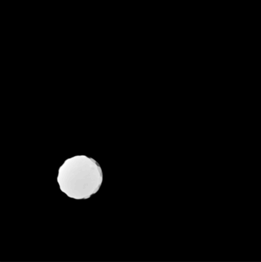
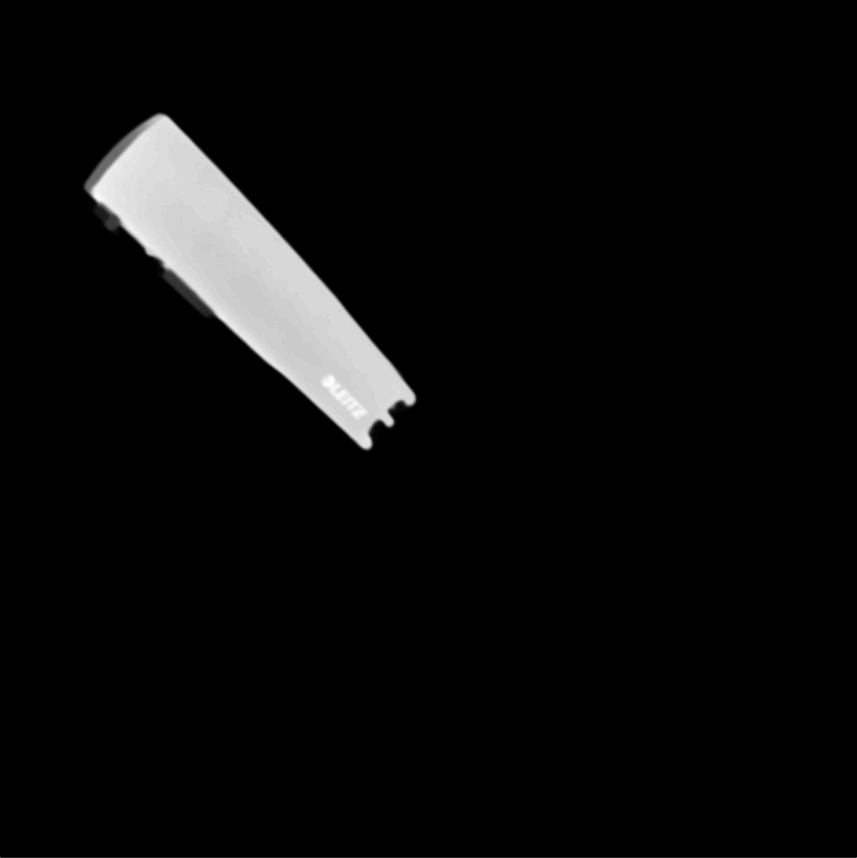
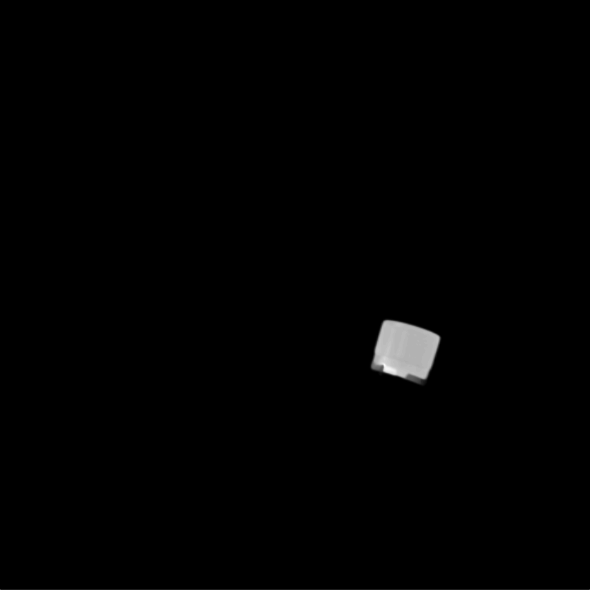
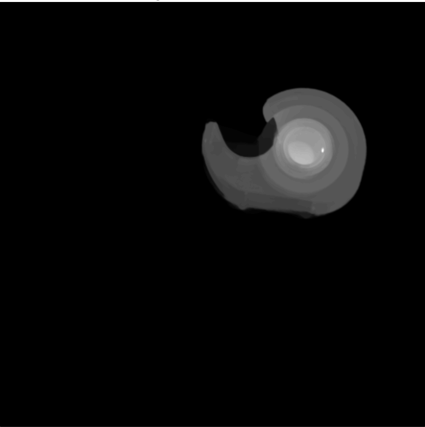
Figure 3: Two-dimensional case. From top left to bottom right: the image $I(x)$, the eigenfunctions $\phi_{1},\,\phi_{2},\,\phi_{3},\,\phi_{4}$ and $\phi_{5}$.

Remark 2.

Since the discretization of the eigenspace problem (9) is highly sparse, and can be computed on a coarse grid, we may compute the eigenfunctions by using a standard restarted Arnoldi iteration Lehoucq:1996:DTI , which results in a very fast algorithm ($\mathcal{O}(n)$). The resulting eigenfunctions are highly sparse as well, see Grote:2016:AEI for details. Hence, we get a good segmentation at a very low cost in terms of run-time and memory requirements.

5 Uses in Medical Imaging

We shall now illustrate the usefulness and versatility of the method through a series of medical imaging examples.

5.1 Segmentation of Medical Images

First we will use a Magnetic Resonance (MR) image of a female breast, taken from eby2008magnetic with permission from, to segment the tumor mass. On the top/right of Fig. 4, we see the first eigenfunction segmenting the tumor perfectly out of the breast image. Next, in the middle row of Fig. 4, we add to the image $I$, $20\%$ of standard Gaussian noise, such that

$$I_{noisy}=I\left(1+\delta\,\xi\right)\,$$ (15)

where $\xi$ is i.i.d. Gaussian random variable with mean zero, variance equal to one and $\delta=0.2$ represents the noise level. Now, we compute the adaptive eigenspace of $I_{noisy}$. Again, the first eigenfunction holds a nice segmentation of the tumor despite the additional noise. To demonstrate the quality of our approach, we consider the image $I$ but this time we destroy the boundaries of the tumor and change them by blurring (using an image manipulation program). The resulting image $I_{blurred}$ is shown on the bottom left of Fig. 4. On the bottom right of Fig. 4, we see the segmentation is accurate and captures the tumor and its blurred boundaries.

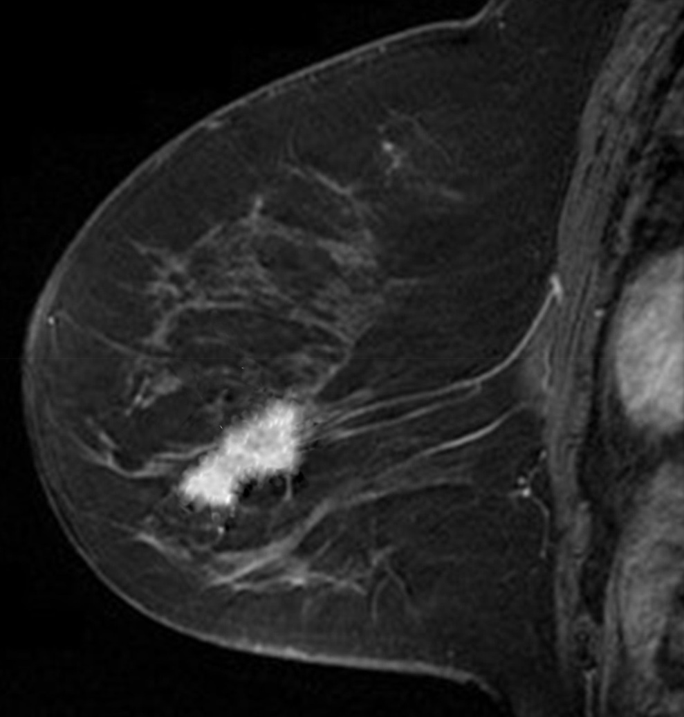
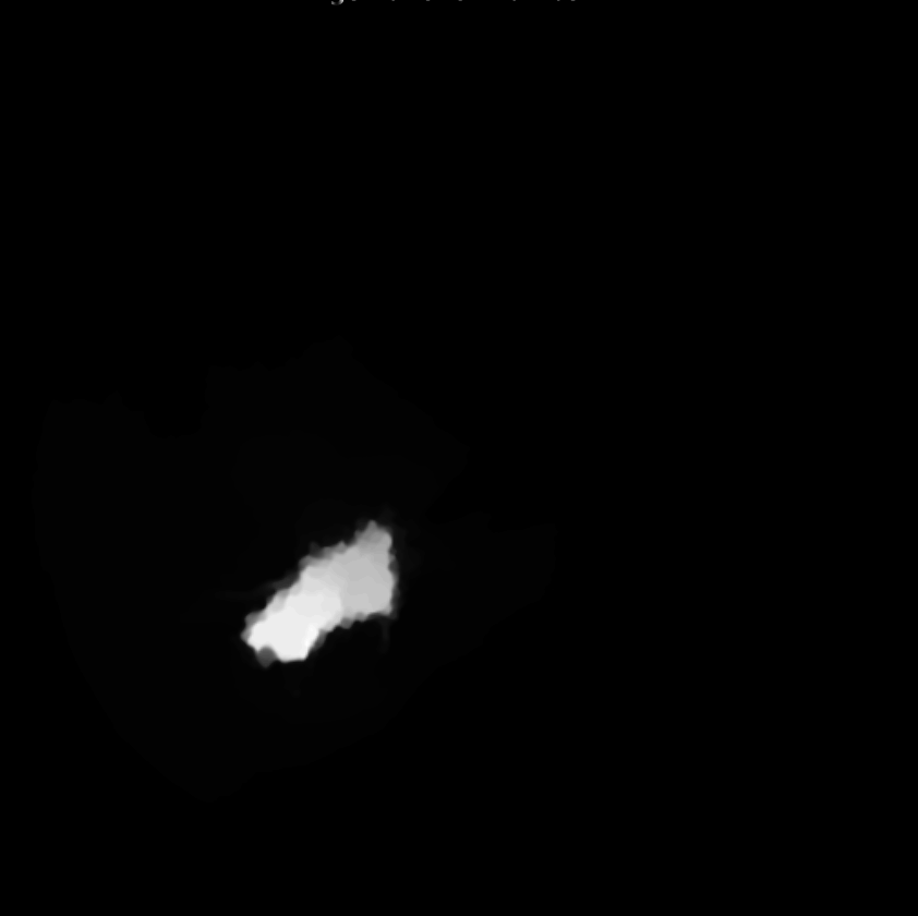
Figure 4: MRI of the breast. Top: the image $I(x)$ and its first eigenfunction $\phi_{1}$. Middle: the image $I_{noise}(x)$ with $20\%$ of added noise and its first eigenfunction $\phi_{1}$. Bottom: the image $I_{blurred}(x)$ with blurred boundaries and its first eigenfunction $\phi_{1}$.

To reduce computational cost and get even more accurate results, we may create a Finite Element (FE) grid on the area of interest rather than on the image boundaries. For illustration, we consider the MR-images $I$ and $I_{blurred}$ shown on the top/left and bottom/left of Fig. 4, respectively. We automatically produce a mesh on the breast boundaries (see on the left of Fig. 5). The segmentation for $I$ and for $I_{blurred}$ is shown on the center and right of Fig. 5, respectively.

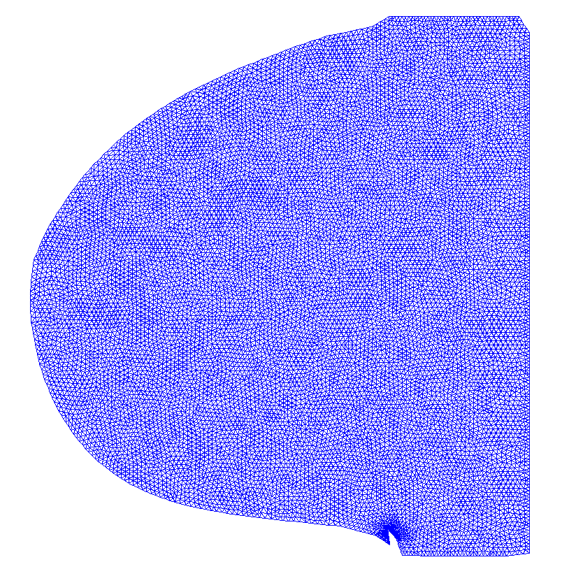
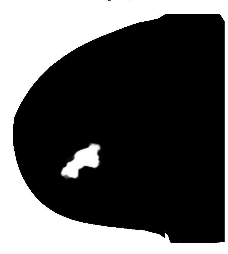
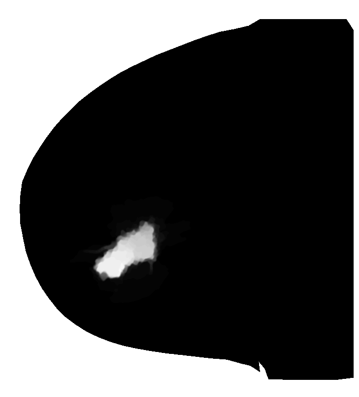
Figure 5: Segmentation of a MR image of the breast using FE: left, the automatically generated FE mesh. Center: the segmentation of the tumor form image $I$. Right, the segmentation of the image $I_{blurred}$ (right) on the FE mesh.

This FE approach can be easily adapted to other images, for example in Fig. 6 left, we apply this approach for segmenting a ventricle MRI heart image, taken from Angenent2006 with permission from¹. In the center of Fig. 6, the FE mesh is shown and on the right of the figure, we see the segmentation of the adaptive eigenspace using FE. As discussed in Rem. 1, we do not always get a binary segmentation, but this is easy to get using a standard threshold.

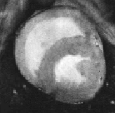
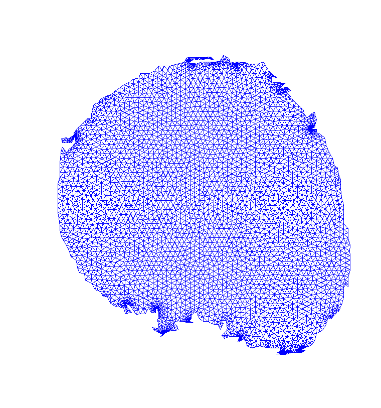
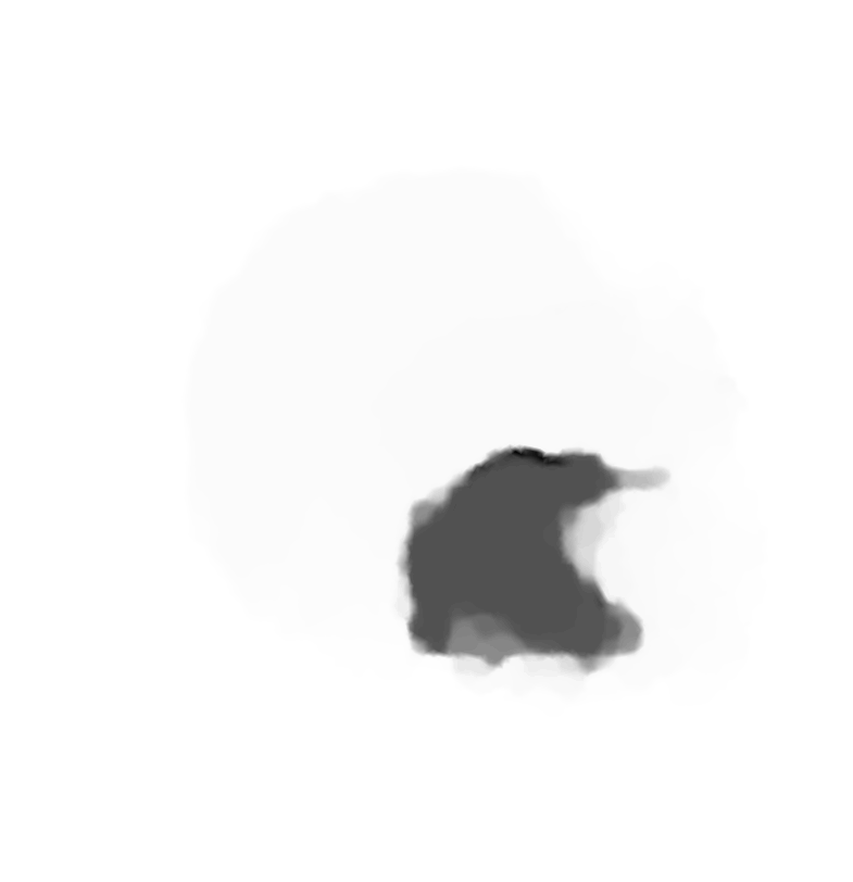
Figure 6: Segmenting MR heart image using FE: left, the MR heart image. Center, the automatically generated FE mesh. Right, the first eigenfunction $\phi_{1}$, i.e. the segmentation of the ventricle (right).

5.2 Noise Removal by Segmenting the Noise Out of an Image

With the following examples we show that the adaptive eigenspace approach can not only be used to segment complicated structures but also to segment out noise and speckle as seen in some medical images. This can be done using (10) with $m\leq K$, where $K$ is the number of eigenfunctions that we include in the expansion of $I$. Here, we take advantage of the fact that the noise/speckle in the image, appears in eigenfunctions correlating to high eigenvalues.

Hence, we truncate the expansion of $I$ to hold only relevant information and take the first $K$ eigenfunctions related to the smallest eigenfunctions. We can approximate $I$ as the following sum

$$\tilde{I}\ =\ I_{0}(x)\ +\ \sum_{m=1}^{K}\beta_{m}\phi_{m}(x),$$ (16)

where $I_{0}$, as defined in (11), holds the information on the boundary of the image and the eigenfunctions $\phi_{m}$ are computed using (9). We have the option to set $I_{0}$ to zero to zero in all or part of the boundary, if we know that the boundary information there is irrelevant.

We consider an OCT B-scan image of a bone piece, shown on the left of Fig. 8. This image is produced by measuring across the cut (yielding the cut profile) while ablating the bone using a laser beam coming from top. In the center and right of Fig. 8, we see the eigenfunctions $\phi_{1}$ and $\phi_{250}$, respectively. It is easy to see that $\phi_{1}$ is extremely relevant to the reconstruction of $\tilde{I}$ and the eigenfunction $\phi_{250}$ holding information only on the noise.

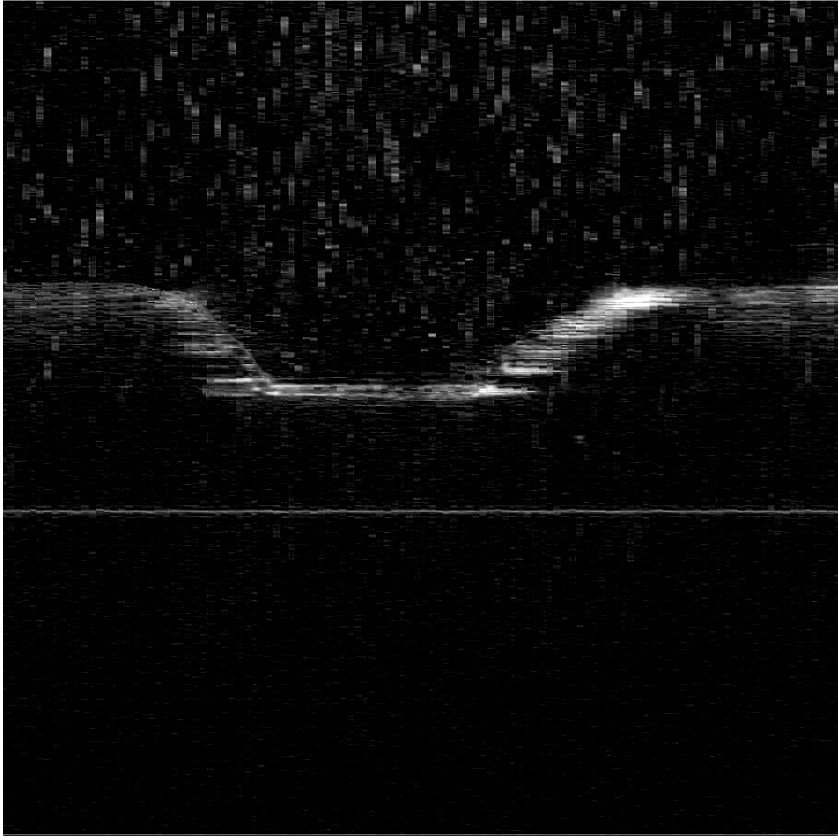
Figure 7: Image filtering: left, the image $I$. Center, the first eigenfunction $\phi_{1}$. Right, the eigenfunction $\phi_{250}$.

Now, we segment the noise out, produced by water droplets of the cooling spray, from the image using (16). The filtered image is shown on the right of Fig. 8.

Figure 8: OCT of a bone: left, the image $I$; right The filtered image $\tilde{I}$ with $K=150$.

Remark 3.

More than $90\%$ of the entries in the eigenfunctions of the adaptive eigenspace are very small, and can be, actually, set to zero without loosing essential information, see Grote:2016:AEI . Hence, the representation of $\tilde{I}$ in (16) is sparse and has low memory requirements.

In some cases the image is so noisy, that we would like to segment the noise out of it before segmenting the image. We consider once more the MR image from Fig. 4 with $120\%$ of added noise (as in (15) with $\delta=1.2$), such that the borders of the tumor are heavily distorted. At the first step, we use the adaptive eigenspace to filter the image (K=150) and then we segment the tumor out of the filtered image. The segmentation is performed with much success, see on the right of Fig. 9. The segmentation is very close to the one done on the original image, without noise, shown on Fig. 4.

Figure 9: MRI of the breast. The image $I(x)$ with $120\%$ of added standard Gaussian noise (left) and the first eigenfunction $\phi_{1}$ of AE of the filtered image $\tilde{I}$ with $K=150$ (right).

6 Concluding Remarks

We have presented a new framework for image segmentation based on the adaptive eigen-space. Instead of minimizing an energy norm and to regularize it, we compute the eigenfunctions of the gradient of the regularization term, to segment an image. The approach has been shown to be insensitive to the parameter $\gamma=\max\left|\nabla I(x)\right|$ as the same value was used for all the experiments reported herein. Hence, the adaptive eigenspace segmentation is not sensitive to the parameter choice and does not need any training or other prior shape information to segment an image other than the image to segment itself.

In addition, we showed how the adaptive eigenspace segmentation can be used to segment the noise out of an image, rather than filtering it with classical methods.

In this paper, mostly medical images are segmented, but clearly, this approach may be directly applied to other type of images. The method uses only a fraction of the computational cost used by other segmentation methods and yet, the results are remarkable. The eigenfunctions are highly sparse and hence this approach can be easily extended to three space dimensions.

Acknowledgment

The authors thank Allen Tannenbaum for useful comments and suggestions.

References

- [1] R. Adams and L. Bischof. Seeded region growing. IEEE Transactions on pattern analysis and machine intelligence, 16(6):641–647, 1994.
- [2] S. Andermatt, S. Pezold, and P. Cattin. Multi-dimensional gated recurrent units for the segmentation of biomedical 3d-data. In International Workshop on Large-Scale Annotation of Biomedical Data and Expert Label Synthesis, pages 142–151. Springer, 2016.
- [3] S. Angenent, E. Pichon, and A. Tannenbaum. Mathematical methods in medical image processing. Bulletin of the American Mathematical Society, 43(3):365–396, 2006.
- [4] Y. Boykov, O. Veksler, and R. Zabih. Fast approximate energy minimization via graph cuts. IEEE Transactions on pattern analysis and machine intelligence, 23(11):1222–39, Nov 2001.
- [5] X. Bresson, S. Esedoḡlu, P. Vandergheynst, J.-P. Thiran, and S. Osher. Fast global minimization of the active contour/snake model. Journal of Mathematical Imaging and vision, 28(2):151–167, 2007.
- [6] V. Caselles, R. Kimmel, and G. Sapiro. Geodesic active contours. International journal of computer vision, 22(1):61–79, 1997.
- [7] T. F. Chan and L. A. Vese. Active contours without edges. IEEE Trans on Image Processing, 10(2):266–77, Feb 2001.
- [8] L. D. Cohen. On active contour models and balloons. CVGIP: Image understanding, 53(2):211–218, 1991.
- [9] M. De Buhan and M. Darbas. Numerical resolution of an electromagnetic inverse medium problem at fixed frequency. Computers & Mathematics with Applications, 2017.
- [10] M. de Buhan and M. Kray. A new approach to solve the inverse scattering problem for waves: combining the TRAC and the Adaptive Inversion methods. Inverse Problems, 29(8):085009, 2013.
- [11] M. de Buhan and A. Osses. A stability result in parameter estimation of the 3D viscoelasticity system. C. R. Acad. Sci. Paris, Ser. I 347:1373–1378, 2009.
- [12] P. R. Eby and C. D. Lehman. Magnetic resonance imaging-guided breast interventions. Topics in Magnetic Resonance Imaging, 19(3):151–162, 2008.
- [13] H. W. Engl, M. Hanke, and A. Neubauer. Regularization of inverse problems, volume 375. Springer Science & Business Media, 1996.
- [14] J. Fan, D. K. Yau, A. K. Elmagarmid, and W. G. Aref. Automatic image segmentation by integrating color-edge extraction and seeded region growing. IEEE transactions on image processing, 10(10):1454–1466, 2001.
- [15] G. Gilboa, M. Moeller, and M. Burger. Nonlinear spectral analysis via one-homogeneous functionals: overview and future prospects. Journal of Mathematical Imaging and Vision, 56(2):300–319, 2016.
- [16] G. H. Golub, P. C. Hansen, and D. P. O’Leary. Tikhonov regularization and total least squares. SIAM Journal on Matrix Analysis and Applications, 21(1):185–194, 1999.
- [17] M. J. Grote, M. Kray, and U. Nahum. Adaptive eigenspace method for inverse scattering problems in the frequency domain. Inverse Problems, 33(2):025006, 2017.
- [18] M. J. Grote and U. Nahum. Adaptive eigenspace regularization for inverse scattering problems. 2017.
- [19] M. Kass, A. Witkin, and D. Terzopoulos. Snakes: Active contour models. International journal of computer vision, 1(4):321–331, 1988.
- [20] S. Kichenassamy, A. Kumar, P. Olver, A. Tannenbaum, and A. Yezzi. Conformal curvature flows: from phase transitions to active vision. Archive for Rational Mechanics and Analysis, 134(3):275–301, 1996.
- [21] R. B. Lehoucq and D. C. Sorensen. Deflation techniques for an implicitly re-started Arnoldi iteration. SIAM J. Matrix Anal. Appl, 17:789–821, 1996.
- [22] G. Litjens, T. Kooi, B. E. Bejnordi, A. A. A. Setio, F. Ciompi, M. Ghafoorian, J. A. van der Laak, B. van Ginneken, and C. I. Sánchez. A survey on deep learning in medical image analysis. arXiv preprint arXiv:1702.05747, 2017.
- [23] U. Nahum. Adaptive eigenspace for inverse problems in the frequency domain. PhD thesis, University of Basel, 2016.
- [24] T. Pavlidis. Segmentation of pictures and maps through functional approximation. Computer Graphics and Image Processing, 1(4):360–372, 1972.
- [25] L. I. Rudin, S. Osher, and E. Fatemi. Nonlinear total variation based noise removal algorithms. Physica D: Nonlinear Phenomena, 60(1):259–268, 1992.
- [26] J. Schmidhuber. Deep learning in neural networks: An overview. Neural networks, 61:85–117, 2015.
- [27] L. Shafarenko, M. Petrou, and J. Kittler. Automatic watershed segmentation of randomly textured color images. IEEE transactions on Image Processing, 6(11):1530–1544, 1997.
- [28] A. N. Tikhonov. On the stability of inverse problems. Dokl. Akad. Nauk SSSR, 39(5):195–198, 1943.
- [29] C. Vogel. Computational Methods for Inverse Problems. Society for Industrial and Applied Mathematics, 2002.
- [30] C. R. Vogel and E. Oman. Iterative methods for total variation denoising. SIAM J. Sci. Comput., 17(1):227–238, 1996.
- [31] J. Wang and W. Huang. Image segmentation with eigenfunctions of an anisotropic diffusion operator. IEEE Transactions on Image Processing, 25(5):2155–2167, May 2016.
- [32] Y. Xu and E. C. Uberbacher. 2d image segmentation using minimum spanning trees. Image and Vision Computing, 15(1):47–57, 1997.