Antagonistic Structural Patterns in Complex Networks

Abstract

Identifying and explaining the structure of complex networks at different scales has become an important problem across disciplines. At the mesoscale, modular architecture has attracted most of the attention. At the macroscale, other arrangements –e.g. nestedness or core-periphery– have been studied in parallel, but to a much lesser extent. However, empirical evidence increasingly suggests that characterizing a network with a unique pattern typology may be too simplistic, since a system can integrate properties from distinct organizations at different scales. Here, we explore the relationship between some of those organizational patterns: two at the mesoscale (modularity and in-block nestedness); and one at the macroscale (nestedness). We analytically show that nestedness can be used to provide approximate bounds for modularity, with exact results in an idealized scenario. Specifically, we show that nestedness and modularity are antagonistic. Furthermore, we evince that in-block nestedness provides a parsimonious transition between nested and modular networks, taking properties of both. Far from a mere theoretical exercise, understanding the boundaries that discriminate each architecture is fundamental, to the extent modularity and nestedness are known to place heavy constraints on the stability of several dynamical processes, specially in ecology.

The detection and identification of emergent structural patterns has been a main focus in the development of modern network theory. Such interest is not surprising, because these arrangements lie at the core of the discipline as one of the keys to the origins –which are the assembly rules that led to an observed pattern?– and dynamics –how is the system’s activity constrained by the structure?– of a network. In addition to these essential questions, the identification of structural signatures is a difficult task per se, which explains as well why so much attention has been put on the technical problem.

Undoubtedly, in this context, modularity Newman and Girvan (2004); Newman (2006) stands out: the organization of a network as a set of cohesive subgroups has, by far, concentrated most of the efforts Duch and Arenas (2005); Blondel et al. (2008); Newman (2004); Leicht and Newman (2008); Barber (2007). Modular architecture is widespread Zachary (1977); Guimerà and Amaral (2005); Eriksen et al. (2003); Adamic and Glance (2005); Fortunato (2010) and responds to the intuition that similar elements in a complex system tend to flock together. However, there are other architectural principles beyond community structure which may play more important roles. In ecology, for instance, scholars have faced the need to define and quantify other patterns, demonstrated to be more relevant in certain scenarios. This is the case of nestedness Atmar and Patterson (1993); Bascompte et al. (2003), a concept that has been crucial to understand the stability and diversity of ecological systems Thébault and Fontaine (2010); Bastolla et al. (2009). Other, more intricate, possibilities have also been explored Lewinsohn et al. (2006); Almeida-Neto et al. (2007), like core-periphery structures Borgatti and Everett (2000); Rombach et al. (2017) –and its extension to the mesoscale Kojaku and Masuda (2017)– are good examples of comparatively less studied architectures.

In these settings, the accent has been mainly placed on designing heuristics and improving algorithms Rombach et al. (2017); Fortunato (2010); Lin et al. (2018); understanding the dynamical constraints that those patterns impose Arenas et al. (2006); Allesina and Tang (2012); or describing plausible microscopic rules that make those patterns emerge Leung and Weitz (2016); Thébault and Fontaine (2010); König et al. (2014); Verma et al. (2016). However, we have very limited knowledge on how different structural signatures may be intertwined, or how –if ever– they affect and limit each other. Indeed, we have examples in which two or more structural features (say, nestedness and modularity) have been jointly considered Olesen et al. (2007); Fortuna et al. (2010); Flores et al. (2011); Borge-Holthoefer et al. (2017). But such consideration overlooked to what extent the inherent constraints of one pattern limit –or boost– the presence of the other. Furthermore, there is extensive evidence that modular and nested architectures play a critical role in relation to the stability of the dynamics of ecological systems Bastolla et al. (2009); Thébault and Fontaine (2010); Stouffer and Bascompte (2011); Allesina et al. (2015), economics Bustos et al. (2012); Saavedra et al. (2011) and social sciences Borge-Holthoefer et al. (2017). Thus, understanding the possibility of coexistence of these structural patterns may shed light on the dynamical trade-offs that either arrangement can facilitate.

In Borge-Holthoefer et al. (2017), the authors observe that modularity and nestedness exhibit an anti-correlated behavior, suggesting that, at least in empirical data, these arrangements hardly coexist. In this work, we depart from this shallow evidence to first explore experimentally, and then analytically, the structural relationship between three structural patterns: nestedness on the macroscopic side, modularity and in-block nestedness at the mesoscale. We analytically characterize these measures in an idealized family of networks, which allows us to precisely derive to what extent the macroscale organization places strict bounds to the emergence of mesoscale patterns. Eventually, we provide soft bound estimations for less restricted scenarios, i.e. real networks.

In a perfectly nested network, the set of neighbors of lower degree nodes are a subset of those with larger degree cit . Such network is typically represented by a presence-absence matrix $a_{ij}$, and the degree of nestedness $\mathcal{{N}}$, can be formally defined as Solé-Ribalta et al. (2018)

$$\mathcal{{N}}=\frac{2}{N_{T}}\left\{\sum_{ij}^{N_{T}}\left[\frac{\mathit{O}_{ij}-\langle\mathit{O}_{ij}\rangle}{k_{j}(N_{T}-1)}\Theta(k_{i}-k_{j})\right]\right\},$$ (1)

where $O_{ij}=\sum_{k}{a_{ik}a_{jk}}$ quantifies the overlap between nodes $i$ and $j$; $k_{i}$ corresponds to the degree of node $i$; and $\Theta(\cdot)$ is the Heaviside step function, that ensures that $O_{ij}$ has a positive contribution when $k_{i}\geq k_{j}$. Additionally, $O_{ij}$ is conveniently corrected by a null model that discounts the expected overlap if links where drawn randomly, $\langle\mathit{O}_{ij}\rangle$. $N_{T}$ is the size of the network.

A modular structure is a rather ubiquitous mesoscale structural organization in which nodes are organized forming groups, i.e. devoting many links to nodes in the same group, and fewer links towards nodes outside. One of the most popular methods to identify communities is through the maximization of the modularity $Q$ Newman and Girvan (2004). The original equation can be rewritten as

$$Q=\sum_{c=1}^{B}\left[\frac{l_{c}}{L}-\left(\frac{d_{c}}{2L}\right)^{2}\right],$$ (2)

where $B$ is the number of communities, $L$ is the total number of links in the network, $l_{c}$ is the total number of links in community $c$, and $d_{c}$ is the sum of the degrees of all nodes in such community.

The possibility of a combined nested-modular organization has been debated in different contexts Flores et al. (2013); Beckett and Williams (2013); Solé-Ribalta et al. (2018). One conceivable form of coexistence is in terms of hybrid structures, as described by Lewinsohn et al. in Lewinsohn et al. (2006). The general layout of these networks is modular, but interactions within each module (or block) are expected to be nested. In contrast, modularity makes no assumption on the internal organization of communities. Worth highlighting, this hybrid structure reframes nestedness, originally a macroscale feature, to the mesoscopic level –it can now be interpreted as an in-block nested structure with $B=1$. The degree of in-block nestedness of a network $\mathcal{I}$ Solé-Ribalta et al. (2018) can be computed as

$$\mathcal{I}=\frac{2}{N_{T}}\left\{\sum_{i,j}^{N_{T}}\left[\frac{\mathit{O}_{ij}-\langle\mathit{O}_{ij}\rangle}{k_{j}(C_{i}-1)}\Theta(k_{i}-k_{j})\delta(\alpha_{i},\alpha_{j})\right]\right\}.$$ (3)

Here, $\alpha_{i}$ represents the community node $i$ belongs to, and $C_{i}$ its size. $\delta(\alpha_{i},\alpha_{j})$ corresponds to the Kronecker delta, equal to one only if nodes $i$ and $j$ belong to the same community.

In order to experimentally assess the dependence between the different presented structural measures, we rely on a probabilistic network generation model Solé-Ribalta et al. (2018). This model is able to generate structures (with and without noise) that smoothly interpolate between the different structural patterns of interest by recourse of 4 parameters: the number of modules $B$, the fraction of inter-modular links $\mu$ (inter-block noise), the fraction of links outside the perfect nested structure $p$ (intra-block noise), and the shape of the nested structure $\xi$ (cf. Supplemental Material).

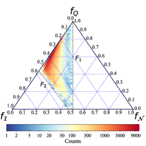
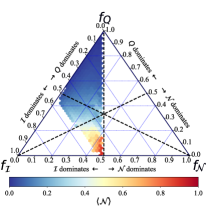
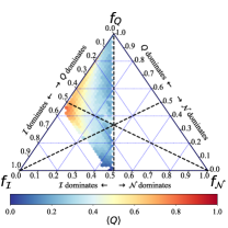
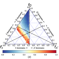
(a)0.2in0.05in (b)0.2in.05in (c)0.2in.05in (d)0.2in.05in

Figure 1: Panel (a) shows the distribution of the generated networks over the ternary plot. The color bar indicates the amounts of networks in each bin. Panels (b), (c) and (d) show the average absolute value of $\mathcal{N}$, $Q$ and $\mathcal{I}$, respectively.

We have measured $\mathcal{N}$, and optimized $Q$ and $\mathcal{I}$ for more than $2\times 10^{5}$ networks on a wide range of parameters: $B\in[1,9]$; $\xi\in[1.5,7]$; $p\in[0,0.6]$; and $\mu\in[0,0.6]$. Restricting $p$ and $\mu$ to $0.6$ allows us to introduce a high level of noise while still preserving some underlying mesoscale structure. For modularity and in-block nestedness optimization, we have used the extremal optimization algorithm Duch and Arenas (2005), adapted to the corresponding objective functions (Eqs. 2 and 3, respectively). Community size of $N_{B}=50$ was assumed, so as we add communities we are also increasing the size of the network, the total number of nodes being $N_{T}=BN_{B}$. Fixing $N_{T}$ and reducing the size of the communities while increasing $B$ produces equivalent results.

Figure 1 shows the results represented over four ternary heatmap plots. A ternary plot, or simplex, is a three-variable diagram in which the sum of the variables is a constant –1 in this case– (for further details cf. Supplemental Material). Panel (a) shows a density plot of the generated networks over the simplex, and the colorbar indicates the amount of networks in each bin of the ternary plot. Relying on these results, it is apparent that the most frequent architecture is predominantly modular. This is expected since most generated networks have blocks ($B>1$), and in-block nested networks are more restrictive, in terms of internal organization, than modular ones. The color code in panels (b), (c) and (d) reports the average absolute value of $\mathcal{N}$, $Q$ and $\mathcal{I}$. Dashed black lines have been added as visual aids to evince dominance regions. A quick glance already shows that the highest values of $\mathcal{N}$ and $Q$ never overlap, while $\mathcal{I}$ bridges between them. This is a valuable insight for the analytical results in the remainder of the article.

Another outstanding feature in Fig. 1 is the existence of sharp boundaries in the ternary plots. The first boundary, $F_{1}$ in panel (a), is induced by the definitions of $\mathcal{N}$ and $\mathcal{I}$: as stated, Eq. 3 reduces to Eq. 1 when $B=1$. Translated to coordinates on the simplex, $F_{1}$ simply reflects that the contribution of $\mathcal{N}$ is always equal or smaller than the contribution of $\mathcal{I}$, $f_{\mathcal{N}}\leq f_{\mathcal{I}}$. More interesting, however, is the existence of $F_{2}$, which suggests that there is an inherent limit that prohibits in-block nestedness to dominate further over $Q$. On close inspection (see Fig. S3 of the Supplemental Materials), networks which map onto $F_{2}$ have high values of $\xi$ and very low values of $p$ and $\mu$. We build on this finding to construct our analytical approach below.

The specific configuration of parameters along $F_{2}$ in Fig. 1 points at a well-defined family of network configurations: a ring of star graphs, $G_{s}$ hereafter. Indeed, an extreme shape parameter ($\xi\to\infty$), perfectly nested intra-block structure ($p=0$) and minimum inter-block connectivity ($\mu\approx 0$) to guarantee a single giant component, render a network model which depends only on $B$, ranging from a single star ($B=1$) to a set of stars ($B>1$) connected with a single link through their central nodes. In other words, $G_{s}$ provides the closest compatible network architecture for the boundary $F_{2}$. Given a ring of star graphs with $B$ communities and $N_{B}$ nodes per community, we can analytically derive the exact values $\mathcal{N}$, $\mathcal{I}$ and $Q$.

Nestedness.

We obtain the analytical expression for $\mathcal{N}$ from the expression in Eq. 1. The pair overlap of a generalist node (the center of each star subgraph), $g$, with a specialist node (periphery of a star), $s$, is $\mathit{O}_{gs}/k_{s}=1$ if $g$ and $s$ belong to the same star (and 0 otherwise). For all those pairs (regardless of the star they belong to), the null model contribution is $\langle\mathit{O}_{gs}/k_{s}\rangle=(N_{B}+1)/BN_{B}$. We can obtain in a similar way the terms for the the generalist-generalist pairs between stars. Summing up all the contributions, the final expression for $\mathcal{N}$ is:

$$\mathcal{N}=\frac{BN_{B}^{3}-BN_{B}^{2}-3BN_{B}+B+2N_{B}+2}{BN_{B}\left(BN_{B}^{2}+BN_{B}-N_{B}-1\right)}.$$ (4)

Modularity.

While the optimal partition for an arbitrary network cannot be easily obtained, this is not the case for $G_{s}$ where each star in the ring forms a community. Thus, we can easily derive the contribution of each star to the total $Q$ following Eq. 2. The first element is $l_{c}=N_{B}-1$. The second element (the amount of links of the network) includes links within and between communities, $L=B(N_{B}-1)+B=BN_{B}$. The last term, the sum of the degrees of all the nodes in community $c$, corresponds to $d_{c}=2N_{B}$. Assembling these, we obtain the modularity of $G_{s}$ as

$$Q =B\left[\frac{N_{B}-1}{BN_{B}}-\left(\frac{2N_{B}}{2BN_{B}}\right)^{2}\right] =1-\frac{1}{N_{B}}-\frac{1}{B},$$ (5)

which is equivalent to the general expression derived in Fortunato and Barthelemy (2007).

In-block nestedness.

The derivation of $\mathcal{I}$ resembles that of $\mathcal{N}$, with the difference that only nodes within the same community contribute; thus, all stars have the same contribution. Focusing now on each star, we have only two contributing terms to the sum: the pair overlap between specialist nodes, $s$, and the pair overlap of the generalist node, $g$, with the specialists. In both cases, the contribution is 1. The null model corrections are $\langle\mathit{O}_{gs}\rangle={k_{g}k_{s}}/{BN_{B}}=(N_{B}+1)/BN_{B}$ and $\langle\mathit{O}_{ss}\rangle={k_{s}k_{s}}/{BN_{B}}={1}/{BN_{B}}$. Finally, the size of the communities is $C_{g}=C_{s}=N_{B}$. Replacing all the contributions in Eq. 3, we obtain

$$\mathcal{I} =1-\frac{3}{BN_{B}}-\frac{2}{N_{B}}.$$ (6)

All the expressions presented above were obtained considering a closed ring, on which the number of intercommunity links is $B$. For the cases $B=1$ and $B=2$, the number of intercommunity links is $B-1$ and the degree of the generalist nodes is $k_{g}=N_{B}-1$ and $k_{g}=N_{B}$, respectively (cf. Supplemental Materials for details on these cases).

We now focus on the bounds that $\mathcal{N}$ and $Q$ impose on each other in some important limits. These correspond to scenarios in which the number of blocks, $B$, and the size of the blocks, $N_{B}$, tend to $\infty$.

We start with $N_{B}\to\infty$. In this case, Eqs. 4 and 5 reduce to

$$\displaystyle\lim_{N_{B}\to\infty}\mathcal{N}=\frac{1}{B}, \displaystyle\lim_{N_{B}\to\infty}Q=1-\frac{1}{B},$$ (7)

which implies that, under these circumstances, $\mathcal{N}$ and $Q$ are complementary –in accordance with the empirical results in Borge-Holthoefer et al. (2017). This result proves analytically the antagonism that exists between these two structural patterns.

With respect to the case $B\to\infty$, Eqs. 4 and 5 turn now

$$\displaystyle\lim_{B\to\infty}\mathcal{N}=0, \displaystyle\lim_{B\to\infty}Q=\frac{N_{B}-1}{N_{B}}.$$ (8)

These results fit the expectation that, with increasing $B$, the negative contribution of non-overlapping nodes through the null model overcomes the decreasing positive contributions realized.

Finally, with respect to in-block nestedness, the analytical calculations in both limits yield

$$\displaystyle\lim_{N_{B}\to\infty}\mathcal{I}=1 \displaystyle\lim_{B\to\infty}\mathcal{I}=\frac{N_{B}-2}{N_{B}}$$ (9)

Noteworthy, the generated synthetic networks follow closely the predictions in limiting cases: Fig. 2 reports the analytical estimation of $\mathcal{N}$, $Q$ and $\mathcal{I}$ (Eqs. 4-6, symbols in the figure) against $B$, and the numerical results for networks generated under different parameters. As the generated networks deviate from the ring of stars $G_{s}$ (i.e. $p>0$ and $\mu>0$), results show a worse fit to the analytical prediction. The mutual bounds that $\mathcal{N}$ and $Q$ impose on each other are obvious, observing a perfectly anti-correlated behavior between nestedness and modularity. Finally, as the networks transition from a nested ($B=1$) to a modular ($B>1$) architecture, the values of in-block nestedness remain very high and almost constant.

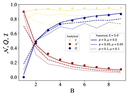
Figure 2: Comparison of the analytical (symbols) and numerical (lines) values of $\mathcal{N}$, $Q$, $\mathcal{I}$ with respect to $B$. All the calculations were performed by taking $N_{B}=50$ and $\xi=5$. The values for $p$ and $\mu$ parameters are indicated in the plot legend.

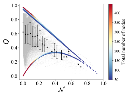
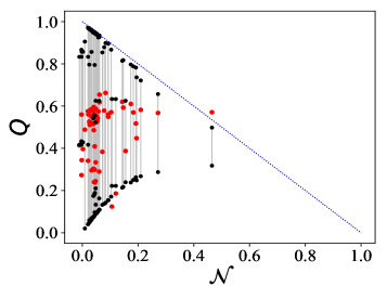
(a)-0.1in0.05in (b) -0.1in0.05in

Figure 3: Panel (a) show the values of $Q$ obtained after optimization (grey dots), plotted against $\mathcal{N}$ for over $2\times 10^{5}$ generated networks and panel (b) for the set of unipartite social network (57 networks) analyzed in Solé-Ribalta et al. (2018). Colored upper and lower bounds of $Q$ have been obtained from Eqs. 5-6 and $B^{*}=f(\mathcal{N},N_{T})$. The color bar indicates the network’s size.

The previous results open a new front to understand the co-occurrence of macro- and mesoscale patterns in complex networks. Complementary to the inherent limits of $Q$ Fortunato and Barthelemy (2007); Lancichinetti and Fortunato (2011), we have now evidence that a certain connectivity arrangement (i.e. nestedness) places hard limits to modularity, at least in extreme settings. This certainty paves the way to obtain estimations for $Q$ prior to computationally costly endeavors: indeed, relaxing those conditions to realistic parameters, soft bounds for $Q$ may be defined. The derivation of these bounds are presented below.

We start from a $G_{s}$ of size $N_{T}=BN_{B}$. From here, Eq. 4 can be rewritten in terms of $N_{T}$ and $B$, and an estimation on the number of blocks as a function of $\mathcal{N}$ and $N_{T}$ can be obtained, i.e. $B^{*}=f(\mathcal{N},N_{T})$. The upper bounds for $Q$ and $\mathcal{I}$ are thus readily available, applying $B^{*}$ to Eqs. 4-5, i.e. assuming that the network structure lies on the boundary $F_{2}$. With the actual measure of $\mathcal{N}$, and upper estimations for $Q$ and $\mathcal{I}$, we can obtain the relative fraction that each measure contributes to the ternary plot along the $F_{2}$ boundary, $f_{\mathcal{N}}^{\uparrow}$, $f_{Q}^{\uparrow}$ and $f_{\mathcal{I}}^{\uparrow}$.

To obtain the lower bounds for $Q$, we observe from Fig. 1(b) that, if we move from boundary $F_{2}$ to boundary $F_{1}$ on the $f_{Q}$-axis direction, i.e. horizontally in Fig. 1, the $\mathcal{N}$ values are approximately constant with respect to the contributions of $Q$ ($f_{Q}^{\uparrow}$ and $f_{Q}^{\downarrow}$). This allows us to make an approximation for the contributions of $Q$ in the ternary plot at $F_{1}$ as $f_{Q}^{\downarrow}\approx f_{Q}^{\uparrow}$. Additionally, we know that $\mathcal{N}=\mathcal{I}$ at boundary $F_{1}$. Thus,

$$f_{Q}^{\downarrow}=\frac{Q}{Q+\mathcal{I}+\mathcal{N}}=\frac{Q}{Q+2\mathcal{N}},$$ (10)

from which a lower bound for $Q$ can be obtained.

Figure 3 shows the values of $Q$ as a function of $\mathcal{N}$ for the previous synthetic ensemble ($\sim 2\times 10^{5}$ networks; panel (a), grey dots); and 57 real unipartite networks (panel (b), red dots) Solé-Ribalta et al. (2018). In panel (a), the values of the theoretical upper and lower bounds are plotted in colors, the color bar indicating the network size. Our approximation of $Q$ bounds is in good agreement with actual values obtained after optimization: most of the optimized $Q$ values lie within the estimated soft bounds. Despite the wide range of parameters –clearly far from limiting cases– estimated upper bounds behave like $Q=1-\mathcal{N}$ almost perfectly. While these bounds are trivial for $\mathcal{N}\approx 0$, we observe that intermediate values of nestedness provide relevant information about the possible mesoscale organization of the network. $Q$ values above the upper bound correspond to networks with a single community $B=1$ and perfectly nested structure, $p=0$ (see Fig. S4). These networks –less than 0.1% of the total– are dense enough to allow a partition with $B>1$ where the nodes of higher degree are gathered in a block, resulting in values of $Q$ larger than expected Solé-Ribalta et al. (2018). Values below the lower bound approximation are more numerous –although still a small fraction of the total. This imprecision shows that there is room to improve the underlying assumption, i.e. that $\mathcal{N}$ values are constant with respect to the contributions of $Q$. In the same spirit, upper and lower bounds for $\mathcal{I}$ can be as well approximated from the actual value of $\mathcal{N}$ (see Fig. S5). For the sake of completeness, $Q$-$\mathcal{I}$ scatter plots are shown in Fig. S6, where we see that $\mathcal{I}$ and $Q$ can coexist, i.e. there is no clear map from one to the other. Remarkably, bound estimation for real networks in Fig. 3(b) closely follows the approximation for synthetic networks: the inferior and superior trends of black dots are the predicted lower and upper bounds. It is worth highlighting, that bound estimation –which has a very low computational cost– renders non-trivial information for some networks ($\mathcal{N}\gtrsim 0.2$).

While the study of macro- and mesoscale arrangements in complex networks has been studied in depth, we know little about how they affect each other. Understanding and, above all, quantifying such pattern interactions becomes necessary for many reasons. First, because empirical evidence suggests the concurrence of more than one pattern within the same network Olesen et al. (2007); Fortuna et al. (2010); Flores et al. (2011); Borge-Holthoefer et al. (2017). Second, because a preliminary approximation of the mesoscale structural features of a network is appealing, at the face of prohibitive costs to analyze very large amounts of data. Further, the interplay between nestedness and modularity is thought fundamental to decipher the dynamical behavior of many empirical systems (like ecological, economic, and technological networks among others). In this work, we have quantified, numerically and analytically, the interference between nestedness (at the macroscale) and modularity and in-block nestedness (at the mesoscale). We show that modularity and nestedness are antagonistic architectures: the growth of one implies the decline of the other, and bounds to modularity can be estimated even in far from idealized settings. Intermediate nested-modular regimes are possible, pointing directly at in-block nested structures as the natural transition between the other two.

References

- Newman and Girvan (2004) M. E. Newman and M. Girvan, Physical review E 69, 026113 (2004).
- Newman (2006) M. E. Newman, Proceedings of the national academy of sciences 103, 8577 (2006).
- Duch and Arenas (2005) J. Duch and A. Arenas, Physical review E 72, 027104 (2005).
- Blondel et al. (2008) V. D. Blondel, J.-L. Guillaume, R. Lambiotte, and E. Lefebvre, Journal of Statistical Mechanics: theory and experiment 2008, 10008 (2008).
- Newman (2004) M. E. Newman, Physical review E 70, 056131 (2004).
- Leicht and Newman (2008) E. A. Leicht and M. E. Newman, Physical review letters 100, 118703 (2008).
- Barber (2007) M. J. Barber, Physical Review E 76, 066102 (2007).
- Zachary (1977) W. W. Zachary, Journal of Anthropological Research 33, 452 (1977).
- Guimerà and Amaral (2005) R. Guimerà and L. A. N. Amaral, Nature 433, 895 (2005).
- Eriksen et al. (2003) K. A. Eriksen, I. Simonsen, S. Maslov, and K. Sneppen, Physical Review Letters 90, 148701 (2003).
- Adamic and Glance (2005) L. A. Adamic and N. Glance, in Proceedings of the 3rd international workshop on Link discovery (ACM, 2005) pp. 36–43.
- Fortunato (2010) S. Fortunato, Physics Reports 486, 75 (2010).
- Atmar and Patterson (1993) W. Atmar and B. D. Patterson, Oecologia 96, 373 (1993).
- Bascompte et al. (2003) J. Bascompte, P. Jordano, C. J. Melián, and J. M. Olesen, Proceedings of the National Academy of Sciences 100, 9383 (2003).
- Thébault and Fontaine (2010) E. Thébault and C. Fontaine, Science 329, 853 (2010).
- Bastolla et al. (2009) U. Bastolla, M. A. Fortuna, A. Pascual-García, A. Ferrera, B. Luque, and J. Bascompte, Nature 458, 1018 (2009).
- Lewinsohn et al. (2006) T. M. Lewinsohn, P. Inácio Prado, P. Jordano, J. Bascompte, and J. M. Olesen, Oikos 113, 174 (2006).
- Almeida-Neto et al. (2007) M. Almeida-Neto, P. R Guimarães Jr, and T. M Lewinsohn, Oikos 116, 716 (2007).
- Borgatti and Everett (2000) S. P. Borgatti and M. G. Everett, Social Networks 21, 375 (2000).
- Rombach et al. (2017) P. Rombach, M. A. Porter, J. H. Fowler, and P. J. Mucha, SIAM Review 59, 619 (2017).
- Kojaku and Masuda (2017) S. Kojaku and N. Masuda, Physical Review E 96, 052313 (2017).
- Lin et al. (2018) J.-H. Lin, C. Tessone, and M. Mariani, Entropy 20, 768 (2018).
- Arenas et al. (2006) A. Arenas, A. Díaz-Guilera, and C. J. Pérez-Vicente, Physical Review Letters 96, 114102 (2006).
- Allesina and Tang (2012) S. Allesina and S. Tang, Nature 483, 205 (2012).
- Leung and Weitz (2016) C. Y. J. Leung and J. S. Weitz, Physical Review E 93, 032303 (2016).
- König et al. (2014) M. D. König, C. J. Tessone, and Y. Zenou, Theoretical Economics 9, 695 (2014).
- Verma et al. (2016) T. Verma, F. Russmann, N. Araújo, J. Nagler, and H. J. Herrmann, Nature Communications 7, 10441 (2016).
- Olesen et al. (2007) J. M. Olesen, J. Bascompte, Y. L. Dupont, and P. Jordano, Proceedings of the National Academy of Sciences 104, 19891 (2007).
- Fortuna et al. (2010) M. A. Fortuna, D. B. Stouffer, J. M. Olesen, P. Jordano, D. Mouillot, B. R. Krasnov, R. Poulin, and J. Bascompte, Journal of Animal Ecology 79, 811 (2010).
- Flores et al. (2011) C. O. Flores, J. R. Meyer, S. Valverde, L. Farr, and J. S. Weitz, Proceedings of the National Academy of Sciences 108, E288 (2011).
- Borge-Holthoefer et al. (2017) J. Borge-Holthoefer, R. A. Baños, C. Gracia-Lázaro, and Y. Moreno, Scientific Reports 7, 41673 (2017).
- Stouffer and Bascompte (2011) D. B. Stouffer and J. Bascompte, Proceedings of the National Academy of Sciences 108, 3648 (2011).
- Allesina et al. (2015) S. Allesina, J. Grilli, G. Barabás, S. Tang, J. Aljadeff, and A. Maritan, Nature Communications 6, 7842 (2015).
- Bustos et al. (2012) S. Bustos, C. Gomez, R. Hausmann, and C. A. Hidalgo, PloS one 7, e49393 (2012).
- Saavedra et al. (2011) S. Saavedra, D. B. Stouffer, B. Uzzi, and J. Bascompte, Nature 478, 233 (2011).
- (36) Without loss of generality, in the following we consider purely unipartite networks. The extension to bipartite ones is trivial.
- Solé-Ribalta et al. (2018) A. Solé-Ribalta, C. J. Tessone, M. S. Mariani, and J. Borge-Holthoefer, Physical Review E 96, 062302 (2018).
- Flores et al. (2013) C. O. Flores, S. Valverde, and J. S. Weitz, The ISME Journal 7, 520 (2013).
- Beckett and Williams (2013) S. J. Beckett and H. T. Williams, Interface Focus 3, 20130033 (2013).
- Fortunato and Barthelemy (2007) S. Fortunato and M. Barthelemy, Proceedings of the National Academy of Sciences 104, 36 (2007).
- Lancichinetti and Fortunato (2011) A. Lancichinetti and S. Fortunato, Physical Review E 84, 066122 (2011).