Limitation of the Lee-Huang-Yang interaction in forming a self-bound state in Bose-Einstein condensates

Abstract

The perturbative Lee-Huang-Yang (LHY) interaction proportional to $n^{3/2}$, where $n$ is the density, creates an infinitely repulsive potential at the center of a Bose-Einstein condensate (BEC) with net attraction, which stops the collapse to form a self-bound state in a dipolar BEC and in a binary BEC. However, recent microscopic calculations of the non-perturbative beyond-mean-field (BMF) interaction indicate that the LHY interaction is valid only for very small values of gas parameter $x$. We show that a realistic non-perturbative BMF interaction can stop collapse and form a self-bound state only in a weakly attractive binary BEC with small $x$ values ($x\lessapprox 0.01$), whereas the perturbative LHY interaction stops collapse for all attractions. We demonstrate these aspects using an analytic BMF interaction with appropriate weak-coupling LHY and strong coupling limits.

1 Introduction

A one-dimensional (1D) bright soliton, formed due to a balance between defocusing forces and nonlinear attraction, can move at a constant velocity [1]. Bright solitons have been studied and observed in different quantum and classical systems, such as, in nonlinear optics [2] and Bose-Einstein condensates (BEC) [3], and in water waves. Usually, 1D bright solitons are analytic with energy and momentum conservation which guarantees mutual elastic collision with shape preservation. Following a theoretical suggestion [4], quasi-1D solitons have been realized [3] in a cigar-shaped BEC with strong transverse confinement. Due to a collapse instability such a soliton in a stationary state cannot be realized [1, 2] in three-dimensions (3D) for attractive interaction. However, a dynamically stabilized non-stationary 3D state can be achieved [5].

The BEC bright solitons are usually studied theoretically with the mean-field Gross-Pitaevskii (GP) equation [6]. It was shown that the inclusion of a perturbative Lee-Huang-Yang (LHY) interaction [7, 8, 9] or of a repulsive three-body interaction [10], both valid in the mean-field domain, generating higher-order repulsive nonlinear terms in the GP equation compared to the cubic nonlinear two-body terms, can avoid the collapse and thus form a self-bound 3D BEC state. Petrov [9] showed that a self-bound binary BEC state can be formed in 3D in the presence of intra-species repulsion with the LHY interaction and an inter-species attraction. Under the same setting a self-bound binary boson-fermion state can be formed in 3D [11]. A self-bound state can also be realized in a multi-component spinor BEC with spin-orbit or Rabi interaction [12]. Self-bound states were observed in dipolar ¹⁶⁴Dy [13] and ¹⁶⁶Er [14] BECs. The formation of self-bound dipolar states was explained by means of the LHY interaction [15, 16, 17, 18]. More recently, a self-bound binary BEC of two hyper-fine states of ³⁹K in the presence of inter-species attraction and intra-species repulsion has been observed [19, 20, 21] and theoretically studied by including the LHY interaction.

The LHY interaction [15, 16, 17, 18, 19, 20, 21, 22, 23], used in stabilizing a 3D self-bound state, is perturbative in nature valid for small values of the gas parameter $x\equiv an^{1/3}$ in the mean-field domain, where $a$ is the scattering length and $n$ the density, and hence has limited validity. For a complete description of the problem, a realistic non-perturbative beyond-mean-field (BMF) interaction should be employed. We use a realistic analytic non-perturbative BMF interaction valid for both small ($x\ll 1,$ weak coupling) and large ($x\gg 1,$ strong coupling) values of the gas parameter which reproduces the result of a microscopic multi-channel calculation of the BMF interaction. For weak coupling, this non-perturbative BMF interaction reduces to the LHY interaction and for strong coupling it has the proper unitarity limit. The LHY interaction leads to a higher-order repulsive quartic non-linearity in the dynamical model compared to the cubic non-linearity of the GP equation.Without this higher-order term, an attractive BEC has an infinite negative energy at the center leading to a collapse of the system to the center. The higher-order repulsive LHY interaction leads to an infinite positive energy at the center and stops the collapse. The realistic non-perturbative BMF interaction does not have such a term except in the extreme weak-coupling limit $(x\lessapprox 0.01)$. For most values of coupling ($+\infty>x>0.1$), such a higher-order nonlinear term is absent in the non-perturbative realistic two-body BMF interaction and a self-bound state cannot be formed. Similar deficiency of the perturbative LHY model in describing self-bound BEC states has been recently pointed out for a binary BEC mixture [24] and for a dipolar BEC [25]. In these cases a three-body interaction can possibly stabilize a self-bound BEC state [10, 11]. We demonstrate our point of view in a study of self-binding in a binary ³⁹K BEC in two different hyper-fine states. We derive the nonlinear model equation with the non-perturbative BMF interaction and solve it numerically. In addition, we consider a variational approximation [26] to this model in the weak-coupling limit with the perturbative LHY interaction for a qualitative understanding.

2 Analytical Formulation

The two-body interaction energy density ${\cal E}$ (energy per unit volume) of a homogeneous dilute weakly repulsive Bose gas including the LHY interaction [7] is given by [9, 10]

$${\cal E}(n,a) = \frac{Un^{2}}{2}\left(1+\frac{2\alpha\sqrt{na^{3}}}{5}\right),\quad\alpha=\frac{64}{3\sqrt{\pi}},$$ (1)

$$= \frac{Un^{2}}{2}+\frac{8m^{4}}{15\pi^{2}\hbar^{3}}c^{5},$$ (2)

where $U=4\pi\hbar^{2}a/m$ is the strength of two-body interaction, $m$ is the mass of an atom, $c=\sqrt{Un/m}$ is the speed of sound in a single-component BEC [6, 27]. A localized BEC of $N$ atoms with number density $n=N|\psi({\bf r},t)|^{2}$, where $\psi({\bf r},t)$ is the wave function at time $t$ and space point $\bf r$ and with interaction (1) is described by the following time-dependent mean-field NLS equation [9, 19, 28] with the perturbative LHY correction:

$${\mathrm{i}}\hbar\frac{\partial\psi({\bf r},t)}{\partial t} =\left[-\frac{\hbar^{2}\nabla^{2}}{2m}+\mu(n,a)\right]\psi({\bf r},t),$$ (3)

$$\mu(n,a) =\frac{\partial{\cal E}}{\partial n}=\frac{4\pi\hbar^{2}an}{m}\left(1+\frac{\alpha}{2}{\sqrt{na^{3}}}\right),$$ (4)

with normalization $\int|\psi|^{2}d{\bf r}=1$ where $\mu(n,a)$ is the chemical potential of the homogeneous Bose gas.

A convenient dimensionless form of Eqs. (1), (3) and (4) can be obtained with the scaled variables ${\bf r}^{\prime}={\bf r}/l_{0}$, $a^{\prime}=a/l_{0}$, $n^{\prime}=nl_{0}^{3},$ $\psi^{\prime}=l_{0}^{3/2}\psi,$ $t^{\prime}=\hbar t/ml_{0}^{2}$, $\mu^{\prime}=\mu ml_{0}^{2}/\hbar^{2}$, etc., with $l_{0}$ a length scale :

$${\cal E}(n,a) =2\pi an^{2}\left(1+\frac{2\alpha}{5}{\sqrt{na^{3}}}\right),$$ (5)

$${\mathrm{i}}\frac{\partial\psi({\bf r},t)}{\partial t} =\left[-\frac{\nabla^{2}}{2}+\mu(n,a)\right]\psi({\bf r},t),$$ (6)

$$\mu(n,a) ={4\pi an}\left(1+\frac{\alpha}{2}{\sqrt{na^{3}}}\right),$$ (7)

where we have dropped the prime from the transformed variables and $n=N|\psi|^{2},\int d{\bf r}|\psi|^{2}=1$.

The $\alpha$-dependent terms in Eqs. (1) and (4) are the lowest-order perturbative LHY corrections to the mean-field energy density and chemical potential and like all perturbative corrections have limited validity for small values of the gas parameter $x\equiv(n^{1/3}a)\ll 1$. For larger values of $x$ the higher-order corrections become important, and specially as $a\to\infty$ at unitarity, the $\alpha$-dependent terms in Eqs. (1) and (4) diverge even faster than the mean-field term proportional to scattering length, while the energy density $\cal E$ and the chemical potential $\mu$ remain finite at unitarity. At unitarity $a\to\infty$, the bulk chemical potential $\mu(n,a)$ cannot be a function of the scattering length $a$ and by dimensional argument should instead be proportional to $n^{2/3}$, e. g., [28]

$$\lim_{a\to\infty}\mu(n,a)=\eta n^{2/3},$$ (8)

where $\eta$ is a universal constant. The corresponding expression for energy density at unitarity is [28]

$$\lim_{a\to\infty}{\cal E}(n,a)=\frac{3}{5}\eta n^{5/3},$$ (9)

with the property $\mu(n,a)=\partial{\cal E}(n,a)/\partial n$.

The following analytic BMF non-perturbative chemical potential with a single parameter $\eta$ valid for both small and large values of gas parameter $x$ is useful for phenomenological application, for example, in the formation of a self-bound state in a binary BEC [28]:

$$\mu(n,a) = n^{2/3}f(x)\equiv n^{2/3}\frac{4\pi(x+\alpha x^{5/2})}{1+\frac{\alpha}{2}x^{3/2}+\frac{4\pi\alpha}{\eta}x^{5/2}},$$ (10)

where $f(x)$ is a universal function with properties $\lim_{x\to 0}f(x)=4\pi x+2\pi\alpha x^{5/2}$ and $\lim_{x\to\infty}f(x)=\eta.$ Consequently, for small and large values of $x$ the chemical potential (10) reduces to the limits (7) and (8), respectively. We will call this model the crossover model, as it is valid for all coupling along the crossover from weak coupling to extreme strong coupling (unitarity). Similarly, an analytic expression for energy density with the correct weak- and strong-coupling limits (5) and (9) is

$${\cal E}(n,a) = n^{5/3}\frac{2\pi(x+\frac{4\alpha}{5}x^{5/2})}{1+\frac{2\alpha}{5}x^{3/2}+\frac{8\pi\alpha}{3\eta}x^{5/2}}.$$ (11)

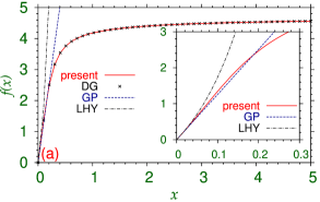
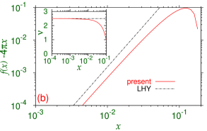
Figure 1: (a) The crossover analytic function $f(x)$ of Eq. (10) with $\eta=4.7$ compared with the realistic multi-channel Hartree calculation of DG [29], the LHY approximation (7), and the GP limit $f(x)=4\pi x$. The inset shows the same for small $x$. (b) A log-log plot of the function $[f(x)-4\pi x]$ versus $x$ for the crossover BMF interaction (10) and its LHY approximation (7). The slope of this plot determines the exponent $\nu$ of the scaling relation $[f(x)-4\pi x]\sim x^{\nu}$. The inset displays the exponent $\nu$ versus $x$ for the two functions. The plotted quantities in this and following figures are dimensionless.

Although there are no precise experimental estimates of the universal constant $\eta$ and the universal function $f(x)$, there are several microscopic calculations of the same [29, 30]. The most recent multi-orbital microscopic Hartree calculation of $\mu(n,a)$ by Ding and Greene (DG) along the weak- ($x\ll 1$) to strong-coupling ($x\gg 1$) crossover yields $\eta=4.7$ [28, 29]. Other microscopic calculations [30] yield $\eta$ in the range from 3 to 9. In Fig. 1(a) we compare the crossover function $f(x)$ of Eq. (10) for $\eta=4.7$ with the same obtained by DG, as well as with the LHY approximation $f(x)=4\pi x+2\pi\alpha x^{5/2}$ and the mean-field GP value $f(x)=4\pi x$. We see that the crossover function $f(x)$ is in full agreement with the microscopic calculation of DG for all $x$. The mean-field GP and the LHY approximations diverge for large $x$ and these two perturbative results are valid in the weak-coupling limit ($x\ll 1$). This is further illustrated in the inset of Fig. 1(a) where we exhibit these functions for small $x$. Even for small $x$ ($x\ll 1$), $f(x)$ of the LHY model could be very different from the non-perturbative interaction (10) and the GP result. Nevertheless, the higher-order $x^{5/2}$ non-linearity in the LHY model will always stop the collapse and allow the formation of a self-bound state, whereas the crossover interaction (10) will stop the collapse only for very small values of $x$, where it tends to the LHY model. To see the higher-order non-linearity in the function $f(x)$ of the crossover model (10), responsible for arresting the collapse, more clearly, we illustrate in Fig. 1(b) the correction to the GP model $[f(x)-4\pi x]$ calculated using the crossover and the LHY interactions versus $x$ in a log-log plot. The slope of this plot gives the power-law exponent $\nu$ of the scaling relation $[f(x)-4\pi x]\sim x^{\nu}$. A large $\nu$ ($>1$) is required to stop the collapse. In the inset of this figure we plot the exponent $\nu$ versus $x$. We find that for the LHY model $\nu=2.5$ for all $x$, but for the realistic crossover model (10) $\nu\approx 2.5$ for $x\lessapprox 0.01$ and then rapidly reduces and has the value $\nu\approx 1$ for $x\approx 0.1$ still for weak-coupling ($x<1$). Hence the LHY model is realistic only for $x\lessapprox 0.01$. In the study of the formation of a self-trapped binary BEC the LHY model should be applied within the domain of its validity.

For a binary BEC, there are two speeds of sound $c_{i}$ [27] for the two components denoted by $i=1,2$ of identical mass $m$, and the energy density can be written as [31]

$${\cal E}(n_{i},a_{i})=\sum_{i}\left[\frac{U_{i}n_{i}^{2}}{2}+\frac{8m^{4}}{15\pi^{2}\hbar^{3}}c_{i}^{5}\right]+U_{12}n_{1}n_{2}$$ (12)

where $n=n_{1}+n_{2}$. Here the two-body intra- and inter-species interaction strengths are $U_{i}=4\pi\hbar^{2}a_{i}/m$ with $a_{i}$ the intra-species scattering length for species $i$, and $U_{12}=4\pi\hbar^{2}a_{12}/m$, where $a_{12}$ is the inter-species scattering length, respectively. The two speeds of sound for this system are [27, 32]

$$c_{i}\equiv c_{\pm}=\sqrt{\frac{\sum_{i}U_{i}n_{i}\pm\sqrt{(U_{1}n_{1}-U_{2}n_{2})^{2}+4n_{1}n_{2}U_{12}^{2}}}{2m}}.$$ (13)

If $a_{12}\approx-\sqrt{a_{1}a_{2}}$ for repulsive intra-species and attractive inter-species interactions, $c_{-}\approx 0$ and $c_{+}=\sqrt{(U_{1}n_{1}+U_{2}n_{2})/m}.$ Then the mean-field energy with LHY interaction for the binary system becomes [33]

$${\cal E}(n_{i},a_{i})=\sum_{i}\frac{U_{i}n_{i}^{2}}{2}+U_{12}n_{1}n_{2}+\frac{8m^{4}}{15\pi^{2}\hbar^{3}}\left(\frac{\sum_{i}U_{i}n_{i}}{m}\right)^{5/2}$$ (14)

We will see that even for weak-coupling ($x<1$), the results for the self-bound binary BEC mixture obtained using the LHY interaction may not be realistic compared to the non-perturbative crossover BMF interaction (10). To demonstrate this we consider a symmetric binary BEC mixture of components $i=1,2$ with an equal number of atoms $N_{1}=N_{2}=N/2$ in the two components, where $N_{i}$ is the number of atoms in component $i$ and $N$ total number of atoms. The binary mean-field equations with the LHY interaction in dimensionless units ($\hbar=m=1$) are [9, 33]

$${\mathrm{i}}\frac{\partial\psi_{1}}{\partial t}=\biggr{[}-\frac{\nabla^{2}}{2}+2\pi Na_{1}|\psi_{1}|^{2}+2\pi Na_{12}|\psi_{2}|^{2}+\frac{\alpha}{\sqrt{2}}\pi N^{3/2}a_{1}\Big{(}\sum_{i}a_{i}|\psi_{i}|^{2}\Big{)}^{3/2}\biggr{]}\psi_{1},$$ (15)

$${\mathrm{i}}\frac{\partial\psi_{2}}{\partial t}=\biggr{[}-\frac{\nabla^{2}}{2}+2\pi Na_{2}|\psi_{2}|^{2}+2\pi Na_{12}|\psi_{1}|^{2}+\frac{\alpha}{\sqrt{2}}\pi N^{3/2}a_{2}\Big{(}\sum_{i}a_{i}|\psi_{i}|^{2}\Big{)}^{3/2}\biggr{]}\psi_{2},$$ (16)

where $\psi_{1}$ and $\psi_{2}$ are wave functions of the two components, normalized as $\int|\psi_{i}({\bf r},t)|^{2}d{\bf r}=1$. The nonlinear terms in Eqs. (15) and (16) are the chemical potentials $\mu_{i}=\partial{\cal E}(n_{i},a_{i})/\partial n_{i}$.

If we further take $a_{1}=a_{2}=a$, $a_{12}=-a-\delta$ and $\psi_{1}=\psi_{2}=\psi$, then Eqs. (15) and (16) become [33]

$${\mathrm{i}}\frac{\partial\psi({\bf r},t)}{\partial t}= \biggr{[}-\frac{\nabla^{2}}{2}-4\pi N{\Big{(}a+\frac{\delta}{2}\Big{)}}|\psi|^{2}+4\pi Na|\psi|^{2}\biggr{(}1+\frac{\alpha}{2}\sqrt{Na^{3}}|\psi|\biggr{)}\biggr{]}\psi({\bf r},t),$$ (17)

where $\psi({\bf r},t)$ is the wave function of the self-bound state containing $N$ atoms and normalized as $\int|\psi({\bf r},t)|^{2}d{\bf r}=1$. Equation (17) is a mean-field equation, with the LHY interaction, satisfied by the self-bound state and is identical to Eq. (1) of Refs. [19, 20] and equivalent to Eq. (10) of Ref. [9] for small $\delta$ . This equation is the same as the single-component mean-field equation (6) with the LHY approximation with an additional attractive nonlinear term $-4\pi N{(a+\delta/2)}|\psi|^{2}$. In both Eqs. (6) and (17) we have $N$ atoms with scattering length $a$. The extra attractive non-linearity in Eq. (17) is of the GP type with scattering length $-(a+\delta/2)$. A self-bound binary state is possible for a positive value of $\delta.$

This close resemblance of the perturbative BMF equation (17) with the NLS equation (6) allows us to include the realistic BMF interaction (10) to the chemical potential. The so-corrected non-perturbative BMF crossover model for the self-bound state is

$${\mathrm{i}}\frac{\partial\psi({\bf r},t)}{\partial t}= \biggr{[}-\frac{\nabla^{2}}{2}-4\pi N{\Big{(}a+\frac{\delta}{2}\Big{)}}|\psi|^{2}+\mu(n,a)\biggr{]}\psi({\bf r},t),$$ (18)

where $\mu(n,a)$ is now given by Eq. (10) with $n=N|\psi|^{2}$ and $\int d{\bf r}|\psi({\bf r},t)|^{2}=1$.

In the following we make a comparative study of the formation of a self-bound binary state using the LHY and crossover models (17) and (18). The result obtained from these two models can be widely different even in the weak-coupling limit $x<1.$ A positive $\delta$ usually leads to a self-bound state in the perturbative LHY model (17), whereas the realistic non-perturbative model (18) leads to a self-bound state only for very small values of the gas parameter $x$ ($x\lessapprox 0.01$), where the exponent $\nu$ is close to 2.5, viz., Fig. 1: for medium values of $x$ in the weak-coupling limit a self-bound state may not be realized in the crossover model (18). The reason is that for an added net attraction the collapse in the LHY model (17) will be stopped by the higher-order quartic LHY non-linearity. In the realistic BMF model (18) this higher-order non-linearity exists only for extreme weak coupling, viz. Fig. 1(b). How a higher-order non-linearity stops the collapse is illustrated next making a variational approximation to the LHY model (17).

The Lagrangian density for Eq. (17) is [33]

$${\cal L}=\frac{N}{2}\Big{\{}{\mathrm{i}}\big{(}\phi\phi^{*^{\prime}}-\phi^{*}\phi^{{}^{\prime}}\big{)}+\big{|}\nabla\phi\big{|}^{2}\Big{\}}-\pi N^{2}\delta|\phi|^{4}+\frac{256\sqrt{\pi}}{15}\big{(}Na\big{)}^{5/2}|\phi|^{5},$$ (19)

where the prime denotes time derivative. This Lagrangian density with the time-derivative terms set equal to zero is the same as the stationary energy density given by Eq. (1) of Ref. [19] under the condition $a_{1}=a_{2}\equiv a$:

$${\cal E}=\frac{N}{2}\big{|}\nabla\phi\big{|}^{2}-\pi N^{2}\delta|\phi|^{4}+\frac{256\sqrt{\pi}}{15}\big{(}Na\big{)}^{5/2}|\phi|^{5}.$$ (20)

A Lagrange variational approximation to Eq. (17) can be performed with the following variational ansatz [26]

$$\phi={\pi^{-3/4}w^{-3/2}}{\exp\Big{(}{-\frac{r^{2}}{2w^{2}}+\text{i}\kappa r^{2}}\Big{)}},$$ (21)

where $w$ is the width and $\kappa$ the chirp. Using this ansatz, the Lagrangian density (19) can be integrated over all space to yield the Lagrangian functional [33]

$$L\equiv\int{\cal L}d{\bf r}={3}\kappa^{2}w^{2}N+\frac{3}{2}w^{2}\kappa^{\prime}N+\frac{3N}{4w^{2}}-\frac{\pi NN\delta}{2\sqrt{2}\pi^{3/2}w^{3}}+\frac{512\sqrt{{2}}\left(Na\right){}^{5/2}}{75\sqrt{5}\pi^{7/4}w^{9/2}}.$$ (22)

The total energy of a self-bound stationary binary BEC is

$$E\equiv\int{\cal E}d{\bf r}=\frac{3N}{4w^{2}}-\frac{\pi NN\delta}{2\sqrt{2}\pi^{3/2}w^{3}}+\frac{512\sqrt{{2}}\left(Na\right){}^{5/2}}{75\sqrt{5}\pi^{7/4}w^{9/2}}.$$ (23)

In the absence of the last term of Eq. (23) with the LHY contribution, the energy $E$ of a stationary state tends to $-\infty$ as $w\to 0$ signaling a collapse instability. However, in the presence of the LHY interaction, the energy at the center ($w=0$) becomes infinitely large $(+\infty)$ and hence a collapse is avoided. The Euler-Lagrange equations of the Lagrangian (22) for variables $\gamma\equiv\kappa,w$,

$$\frac{\partial}{\partial t}\frac{\partial L}{\partial\gamma^{\prime}}-\frac{\partial L}{\partial\gamma}=0,$$ (24)

lead to

$$w^{\prime\prime}=\frac{1}{w^{3}}-\frac{N\delta}{\sqrt{2\pi}w^{4}}+\frac{512\sqrt{2N^{3}a^{5}}}{25\sqrt{5}\pi^{7/4}w^{11/2}},$$ (25)

which describes the variation of the width of the self-bound state with time. The width of a stationary state is obtained by setting $w^{\prime\prime}=0$ in Eq. (25).

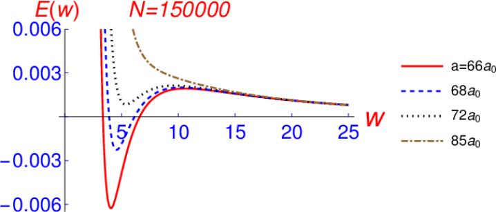
Figure 2: Variational energy per atom $E(w)=E/N$, viz. Eq. (23), as a function of width for $N=150000,$ $a=66a_{0},68a_{0},72a_{0},$ and $85a_{0}$, and $\delta=4a_{0}$. The negative-energy minima for $a=66a_{0},68a_{0}$ correspond to a stable state and the positive-energy minimum for $a=72a_{0}$ denotes a meta-stable state. The minimum has disappeared for $a=85a_{0}$ indicating an unbound configuration.

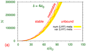
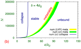
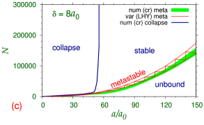
Figure 3: Stable, meta-stable (meta), unbound and collapse regions highlighted in the $N-a$ phase plots. Results of (a) numerical (num) calculation and variational (var) approximation based on the LHY model (17) with $\delta=4a_{0}$, (b) numerical calculation based on the LHY and crossover (cr) models (17) and (18) with $\delta=4a_{0}$, (c) numerical calculation and variational approximation based on the LHY and crossover models (17) and (18) with $\delta=8a_{0}$. The region marked “collapse” denotes collapse of the system only for the non-perturbative BMF crossover model (18).

3 Numerical Result

The effective nonlinear equation (18) does not have analytic solution and different numerical methods, for example, split-step Crank-Nicolson [34] or pseudo-spectral [35] method, are employed for its solution. We use split time-step Crank-Nicolson method to solve Eq, (18) numerically [36]. The minimum-energy ground-state solution for the self-bound state is obtained by evolving the trial wave functions, chosen to be Gaussian, in imaginary time $\tau=it$ as is proposed in Ref. [34]. The numerical results of the models for stationary self-bound state (17) and (18) in a spherically symmetric configuration are presented and critically contrasted in the following in spherical coordinate $r$. We consider spatial and time steps, to solve the NLS equations in imaginary-time propagation, as small as $r=0.0125$ and $t=10^{-5}$ and take the length scale $l_{0}=1$ $\mu$m throughout this study. A small space step is needed to find out the possible collapse of the self-bound state when its size becomes very small.

We consider a binary self-bound state consisting of $|m_{F}=-1\rangle$ and $|m_{F}=0\rangle$ hyper-fine states of ³⁹K with an equal number $N/2$ of atoms in the two states, which has been realized experimentally [19, 20]. The intra-species scattering lengths of the two components can be varied by a Feshbach resonance [37] resulting in a variation of the scattering length $a=\sqrt{a_{1}a_{2}}$.. These scattering lengths are kept quite close to each other and we take $a=\sqrt{a_{1}a_{2}}\approx a_{1}\approx a_{2}$. The inter-species scattering length $a_{12}$ is taken as $a_{12}=-a-\delta$ with $\delta=4a_{0}$ and $8a_{0}$ covering the range of $\delta$ values considered in the experiment [19]: $\delta=2.4a_{0},3.2a_{0},3.8a_{0},4.4a_{0},5a_{0}$ and $5.5a_{0}$ with $a_{0}$ the Bohr radius. In this model study we will vary $a$ and contrast the results obtained with models (17) and (18).

The variational result for energy with the LHY interaction (23) confirm the existence of energetically meta-stable as well as stable self-bound states. To illustrate the distinction between a meta-stable and a stable state, the variational energy per atom $E(w)\equiv E/N$ of binary self-bound states are displayed in Fig. 2 as a function of the variational width $w$ for $N=150000$, $\delta=4a_{0},$ and $a=66a_{0},68a_{0},72a_{0},$ and $85a_{0}$. In Fig. 2, a meta-stable state corresponds to a curve with a local minimum in the energy (at a positive energy), viz. $a=72a_{0}$, whereas a stable state corresponds to the curve with a global minimum (at a negative energy), viz. $a=66a_{0},68a_{0}$. The energy, as $w\to\infty$, is zero. An unbound state corresponds to a curve with no minimum, viz. $a=85a_{0}$ in Fig. 2. All states for $a<66a_{0}$ are stable, and those with $a>85a_{0}$ are unbound.

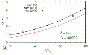
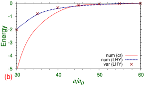
Figure 4: Results of numerical (num) calculation and variational (var) approximation to (a) root mean square radius and (b) energy $E/N$ based on the LHY model (17) and crossover (cr) model (18) with $\delta=4a_{0}$ and $N=100000$.

The variational phase plot in the $N-a$ plane of the formation of a self-bound binary BEC state with the perturbative LHY model (17), while keeping $\delta$ fixed at $4a_{0}$, is illustrated in Fig. 3(a). The variational phase plot is obtained by exploring the minimum of variational energy (23). The region marked stable corresponds to global minima of energy whereas meta-stable to local minima of energy. In the region marked unbound, there is no minima of energy. The meta-stable states appear in a region separating the whole phase space into two parts: stable and unbound. In this plot we also exhibit the result obtained from a numerical solution of Eq. (17) with the LHY interaction. A similar phase plot based on a numerical solution of Eq. (18) with non-perturbative BMF interaction (10) is shown in Fig. 3(b) for $\delta=4a_{0}$. For very small values of the gas parameter $x=na^{1/3}$, this phase plot agrees with that in Fig. 3(a). For slightly larger values of the gas parameter, we have seen that the $x^{\nu},\nu=2.5$ divergence of the universal function $f(x)$ (10), responsible for stopping collapse, disappears from the BMF interaction (10), viz. Fig. 1(b), and this happens for $x>0.1$. Once this happens, the system collapses. The collapse region is illustrated in Fig. 3(b) for the BMF interaction (10), which is clearly absent in the case of the perturbative LHY interaction in Fig. 3(a). For a fixed $\delta$, the collapse takes place for small $a$ due to a reduced repulsion. The self-bound state shrinks to a small size with higher density $n$ thus pushing $x=an^{1/3}$ beyond 0.1 and causing the self-bound state to collapse. The collapse instability is expected to be enhanced as the scattering length imbalance $\delta$ increases, consequently increasing the attraction and pushing the gas parameter $x$ beyond $x=0.1$. Once this happens the non-perturbative BMF interaction (18) will not stop the collapse. Thus with added attraction the domain of collapse has increased in Fig. 3(c) for $\delta=8a_{0}$, compared to Fig. 3(b) with $\delta=4a_{0}$. The unbound domain has also reduced in Fig. 3(c) with added attraction. With further increase of $\delta$ the collapse region increases.

In Fig. 4 we plot (a) root mean square radius $\langle r\rangle$ and (b) energy $E/N$ of the self-bound states for $\delta=4a_{0}$ and $N=100000$ for values of $a$ where a stable state can be formed in the non-perturbative BMF model (18). We find that results for the non-perturbative and perturbative models qualitatively agree where a self-bound state can be formed. The energy of the crossover model in Fig. (4)(b) rapidly decreases as the scattering length $a$ is reduced signaling a collapse. In the experiment of Semeghini et al. [21] the value of $\delta$ was kept very small and it was found that with the increase of $\delta$ the size of the binary self-bound state was drastically reduced before it was quickly destroyed [38]. However, they did not study the fate of the state. Nevertheless, this behavior signals a collapse. The three-body loss is a steady slow process, which will lead to a slower destruction of the self-bound state. The value of $\delta$ was also kept small around $3a_{0}$ in the experiment of Cabrera et al. [19].

4 Conclusion

We studied the formation of a self-bound state in a binary BEC using a realistic non-perturbative BMF interaction (10) and critically compared the results with those obtained using the perturbative LHY interaction (7). We find that a self-bound state can be formed only for weakly attractive systems, where both interactions could stop the collapse. For stronger attraction, the unrealistic LHY interaction continues to stop the collapse, whereas the realistic BMF interaction could not stop collapse and create a self-bound state. For an analysis of the self-bound BEC, a realistic non-perturbative BMF interaction should be used in place of the perturbative LHY interaction, which could lead to an inappropriate description.

The present derivation of the BMF interaction (10) is heuristic, rather than rigorous, in nature and has a single parameter $\eta$ fitted to the plausible result of a microscopic calculation by Ding and Greene [29]. Also, to keep the underlying model simple, in this application we considered a special case of a binary BEC with equal number of atoms $N_{i}$ and equal intra-species scattering lengths $a_{i}$ in the two components. Nevertheless, the disappearance of the LHY repulsion for values of the gas parameter $x\gtrapprox 0.01$ and the inability of the BMF interaction to stop the collapse and support a self-bound state are independent of the present derivation and subsequent calculation. Similar conclusions demonstrating the deficiency of the LHY interaction to explain the properties of a self-bound state unconditionally in a binary [24] and in a dipolar BEC [25] are in agreement with the conclusions of the present paper. Our finding is in agreement with the recent comparison of the LHY approximation, Monte Carlo simulations, and experiments on self-bound droplets in a dipolar gas [25] demonstrating that the Monte Carlo simulations agree well with experiments, while the LHY approximation does not provide good agreement, being unable to reproduce the observable properties of the quantum droplets. Hence in spite of the heuristic derivation of our model and the special binary mixture considered here, we do not believe our conclusions to be so peculiar as to have no general validity. Although we illustrated our findings for a binary BEC mixture, the conclusions will be applicable in general, for example, in the formation of a self-bound state in a dipolar BEC [13] or in a binary boson-fermion mixture [11].

References

References

- [1] Y. S. Kivshar and B. A. Malomed, Rev. Mod. Phys. 61 (1989) 763; V. S. Bagnato, D. J. Frantzeskakis, P. G. Kevrekidis, B. A. Malomed, D. Mihalache, Rom. Rep. Phys. 67 (2015) 5; D. Mihalache, Rom. J. Phys. 59 (2014) 295.
- [2] Y. S. Kivshar and G. Agrawal, Optical Solitons: From Fibers to Photonic Crystals, (Academic Press, San Diego, 2003).
- [3] K. E. Strecker, G. B. Partridge, A. G. Truscott, R. G. Hulet, Nature 417 (2002) 150; L. Khaykovich, F. Schreck, G. Ferrari, T. Bourdel, J. Cubizolles, L. D. Carr, Y. Castin, C. Salomon, Science 256 (2002) 1290; S. L. Cornish, S. T. Thompson, C. E. Wieman, Phys. Rev. Lett. 96 (2006) 170401.
- [4] V. M. Pérez-García, H. Michinel, H. Herrero, Phys. Rev. A 57 (1998) 3837.
- [5] S. K. Adhikari, Phys. Rev. A 69 (2004) 063613.
- [6] F. Dalfovo, S. Giorgini, L. P. Pitaevskii, S. Stringari, Rev, Mod. Phys. 71(1999) 463; V. I. Yukalov, Laser Phys. 26 (2016) 062001; V. I. Yukalov, Laser Phys. 23 (2013) 062001.
- [7] T. D. Lee and C. N. Yang, Phys. Rev. 105 (1957) 1119; T. D. Lee, K. Huang, C. N. Yang, Phys. Rev. 106 (1957) 1135; T. D. Lee and C. N. Yang Phys. Rev. 117 (1960) 12.
- [8] A. R. P. Lima and A Pelster, Phys. Rev. A 84 (2011) 041604(R); A. R. P. Lima and A Pelster, Phys. Rev. A 86 (2012) 063609.
- [9] D. S. Petrov, Phys. Rev. Lett. 115 (2015) 155302.
- [10] S. K. Adhikari, Phys. Rev. A 95 (2017) 023606.
- [11] S. K. Adhikari, Laser Phys. Lett. 15 (2018) 095501; D. Rakshit, T. Karpiuk, M. Brewczyk, M, Gajda, arXiv:1801.00346.
- [12] S. Gautam and S. K. Adhikari, Phys. Rev. A 97 (2018) 013629; S. Gautam and S. K. Adhikari, Phys. Rev. A 95 (2017) 013608; Y.-C. Zhang, Z.-W. Zhou, B. A. Malomed, H. Pu, Phys. Rev. Lett. 115 (2015) 253902; Y. Li, Z. Luo, Y. Liu, Z. Chen, C. Huang, S. Fu, H. Tan, B. A. Malomed, New J. Phys. 19 (2018) 113043; A. Cappellaro, T. Macri, G. F. Bertacco, L. Salasnich, Sci. Rep. 7 (2017) 13358; A. Cappellaro, T. Macri, L. Salasnich, Phys. Rev. A 97 (2018) 053623; A. Cidrim, F. E. A. dos Santos, E. A. L. Henn, T. Macri, Phys. Rev. A 98 (2018) 023618; A. Boudjemaa, Phys. Rev. A 98 (2018) 033612; F. Ancilotto, M. Barranco, M. Guilleumas, M. Pi, Phys. Rev. A 98 (2018) 053623.
- [13] H. Kadau, M. Schmitt, M. Wenzel, C. Wink, T. Maier, I. Ferrier-Barbut, and T. Pfau, Nature 530 (2016) 194.
- [14] L. Chomaz, S. Baier, D. Petter, M. J. Mark, F. Wächtler, L. Santos, F. Ferlaino, Phys. Rev. X 6 (2016) 041039.
- [15] F. Wächtler and L. Santos Phys. Rev. A 93 (2016) 061603(R).
- [16] M. Schmitt, M. Wenzel, F. Böttcher, I. Ferrier-Barbut, T. Pfau, Nature 539 (2016) 259.
- [17] I. Ferrier-Barbut, H. Kadau, M. Schmitt, M. Wenzel, T. Pfau, Phys. Rev. Lett. 116 (2016) 215301.
- [18] R. N. Bisset, R. M. Wilson, D. Baillie, P. B. Blakie Phys. Rev. A 94 (2016) 033619.
- [19] C. R. Cabrera, L. Tanzi, J. Sanz, B. Naylor, P. Thomas, P. Cheiney, L. Tarruell, Science 359 (2018) 301.
- [20] P. Cheiney, C. R. Cabrera, J. Sanz, B. Naylor, L. Tanzi, L. Tarruell, Phys. Rev. Lett. 120 (2018) 135301.
- [21] G. Semeghini, G. Ferioli, L. Masi, C. Mazzinghi, L. Wolswijk, F.Minardi, M. Modugno, G. Modugno, M. Inguscio, M. Fattori, Phys. Rev. Lett. 120 (2018) 235301.
- [22] G. Ferioli, G. Semeghini, L. Masi, G. Giusti, G. Modugno, M. Inguscio, A. Gallemí, A. Recati, M. Fattori, Phys. Rev. Lett. 122 (2019) 090401.
- [23] R. Schützhold, M. Uhlmann, Yan Xu, U. R. Fischer, Int. J. Mod. Phys. B 20 (2006) 3555.
- [24] C. Staudinger, F. Mazzanti, R. E. Zillich, Phys. Rev. A 98 (2018) 023633.
- [25] F. Böttcher, M. Wenzel, J.-N. Schmidt, M. Guo, T. Langen, I. Ferrier-Barbut, T. Pfau, R. Bombín, J. Sánchez-Baena, J. Boronat, and F. Mazzanti, arXiv:1904.10349 (2019)
- [26] V. M. Perez-Garcia, H. Michinel, J. I. Cirac, M. Lewenstein, P. Zoller, Phys. Rev. A 56 (1997) 1424.
- [27] C. J. Pethick and H. Smith, Bose Einstein condensation in Dillute Gases, Second Edition, (Cambridge University Press, Cambridge, 2008).
- [28] S. K. Adhikari and L. Salasnich, Phys. Rev. A 78 (2008) 043616; S. K. Adhikari and L. Salasnich, Sci. Rep. 8 (2018) 8825.
- [29] Y. Ding and C. H. Greene, Phys. Rev. A 95 (2017) 053602.
- [30] J. L. Song and F. Zhou, Phys. Rev. Lett. 103, 025302 (2009); Yu-Li Lee and Yu-Wen Lee, Phys. Rev. A 81 (2010) 063613; J. M. Diederix, T. C. F. van Heijst, H. T. C. Stoof, Phys. Rev. A 84 (2011) 033618; F. Zhou and M. S. Mashayekhi, Ann. Phys. 328 (2013) 83; M. Rossi, L. Salasnich, F. Ancilotto, F. Toigo, Phys. Rev. A 89 (2014) 041602.
- [31] A. Eckardt, C. Weiss, M. Holthaus, Phys. Rev. A 70 (2004) 043615.
- [32] Yu. G. Gladush, A. M. Kamchatnov, Z. Shi, P. G. Kevrekidis, D. J. Frantzeskakis, and B. A. Malomed, Phys. Rev. A 79, 033623 (2009).
- [33] S. Gautam and S. K. Adhikari, J. Phys. B 52 (2019) 055302.
- [34] P. Muruganandam and S. K. Adhikari, Comput. Phys. Commun. 180 (2009) 1888; L. E. Young-S., D. Vudragović, P. Muruganandam, S. K. Adhikari, A. Balaž, Comput. Phys. Commun. 204 (2016) 209; L. E. Young-S., P. Muruganandam, S. K. Adhikari, V. Lončar, D. Vudragović, A. Balaž, Comput. Phys. Commun. 220 (2017) 503.
- [35] P. Muruganandam and S. K. Adhikari, J. Phys. B 36 (2003) 2501.
- [36] D. Vudragović, I. Vidanović, A. Balaž, P. Muruganandam, S. K. Adhikari, Comput. Phys. Commun. 183 (2012) 2021; B. Satarić, V. Slavnić, A. Belić, A. Balaž, P. Muruganandam, S. K. Adhikari, Comput. Phys. Commun. 200 (2016) 411; R. Kishor Kumar, L. E. Young-S., D. Vudragović, Antun Balaž, P. Muruganandam, S. K. Adhikari, Comput. Phys. Commun. 195 (2015) 117; V. Lončar, L. E. Young-S., S. Škrbić, P. Muruganandam, S. K. Adhikari, A. Balaž, Comput. Phys. Commun. 209 (2016) 190; V. Lončar, A. Balaž, A. Bogojević, S. Škrbić, P. Muruganandam, S. K. Adhikari, Comput. Phys. Commun. 200 (2016) 406.
- [37] S. Inouye, M. R. Andrews, J. Stenger, H.-J. Miesner, D. M. Stamper-Kurn, W. Ketterle, Nature 392 (1998) 151.
- [38] M. Fattori, private communication, (2019).