Near-Optimal Coded Apertures for Imaging via Nazarov’s Theorem

Abstract

We characterize the fundamental limits of coded aperture imaging systems up to universal constants by drawing upon a theorem of Nazarov regarding Fourier transforms. Our work is performed under a simple propagation and sensor model that accounts for thermal and shot noise, scene correlation, and exposure time. Focusing on mean square error as a measure of linear reconstruction quality, we show that appropriate application of a theorem of Nazarov leads to essentially optimal coded apertures, up to a constant multiplicative factor in exposure time. Additionally, we develop a heuristically efficient algorithm to generate such patterns that explicitly takes into account scene correlations. This algorithm finds apertures that correspond to local optima of a certain potential on the hypercube, yet are guaranteed to be tight. Finally, for i.i.d. scenes, we show improvements upon prior work by using spectrally flat sequences with bias. The development focuses on 1D apertures for conceptual clarity; the natural generalizations to 2D are also discussed.

Index Terms—  coded aperture cameras, computational photography, optical signal processing, Fourier analysis

1 Introduction

Certain modern imaging systems, especially those operating at high frequencies, use coded apertures. In these systems, a spatial mask that selectively blocks light from reaching the sensor is used as opposed to a traditional lens. The scene is then recovered by suitable post-processing. Perhaps the earliest and simplest instance of coded aperture imaging is the pinhole structure; see, e.g., [1] for a survey. The development of X-ray and gamma-ray astronomy gave rise to more sophisticated coded apertures [2, 3] to get around the lack of lenses and mirrors in such settings. Both proposed using random blockage patterns with a specified mean transmittance as a method to increase the aperture size as compared to the classical pinhole while retaining its resolution benefits.

More modern developments include the usage of uniformly redundant arrays (URA) to improve upon random on-off patterns [4], anti-pinhole imaging [5], as well as the combining of mask and lens in order to, e.g., facilitate depth estimation [6], deblur out-of-focus elements in an image [7], enable motion deblurring [8], and/or recover 4D lightfields [9]. Even more recent work seeks to forgo lenses altogether to decrease costs and meet physical constraints [10, 11]. Understanding coded apertures is also relevant in non-line-of-sight applications where masks naturally occur as scene occlusions [12, 13].

In light of the increased importance of coded apertures, prior work [14] described a model under which they can be analyzed. This model uses far-field geometric optics to model light propagation and a sensor model that includes thermal and shot noise components. Together with mutual information (MI) as a performance metric, [14] compared the classical random on-off apertures [2, 3] of varying intensity to the “spectrally flat” patterns with transmissivity $1/2$ (same as the URA of [4]). Among other things, the analysis showed that when shot noise dominates thermal noise, randomly generated masks with lower transmissivity than $1/2$ offered greater performance compared to spectrally flat patterns of transmissivity $1/2$.

This paper extends the work of [14] in multiple respects that may be broadly grouped into the following three main contributions.

First, we refine the model of [14] by incorporating exposure time. Here, we analyze linearly-constrained minimum mean square error (LMMSE) estimatation as opposed to MI given its direct operational relevance, though we remark in advance that our conclusions carry over to the MI criterion used in [14]; see Sec. 4.

Second, we remark upon the existence and construction of spectrally flat sequences with transmissivities $1/8,1/4$ in addition to $1/2$. This extends the range of parameters where we have a sharp characterization of optimal coded apertures in our framework, and gives a tight answer to the problem of optimal coded apertures for i.i.d. scenes; see Props. 2,  3 for precise statements.

Third, we provide optimal (up to a universal constant) coded apertures, both in 1D as well as in 2D, applicable for any prior on the spectrum of the scene at hand. The sense of tightness of the optimality is given precisely in Prop. 4. This includes (but is not limited to) the naturally occuring power law [15]($f^{-\gamma}$-prior). Our aperture design naturally varies depending on the choice of prior, and we provide a (heuristically) efficient greedy algorithm for their generation. Essentially all the required mathematical results stem from a beautiful theorem of Nazarov [16, p. 5] combined with classical waterfilling for spectrum allocation. We note that [17, pp. 9-11] has identified other applied problems for which Nazarov’s theorem provides conceptual clarity and/or solutions.

2 Model

We first describe our model, and discuss how it differs from that in [14]. We use the standard Poisson model of classical optics for photon counting, and emphasize its dependence on the exposure time $t$. The analysis of MI under Poisson models is cumbersome, and even with mean square error (MSE) it is often unclear how to achieve optimal MSE in practice. As such, the standard estimation process is linear; indeed, the work of [2, 3] used correlation decoders. In fact, both  [2, 3] give beautiful analog realizations of such a decoder. Accordingly, we emphasize LMMSE. We note that if one used a Gaussian model instead, LMMSE is the same as MSE, and MSE is in turn essentially equivalent to MI in the low SNR limit [18, 19]. LMMSE depends purely on first and second moments, so in our mathematical study we do not emphasize the specific Poisson statistics.

We use a 1D model, as in [14], to simplify the exposition of the concepts and results. We emphasize that all of the results of this paper generalize naturally to the analogous 2D model, whose discussion we defer to Sec. 4.

Let $\mathbf{f}$ denote the intensities of the unknown 1D scene of length $n$ of expected total power $J$. Let $\operatorname*{\mathbb{E}}[\mathbf{f}]=(J/n)\mathbf{1},\operatorname*{\mathbf{Cov}}[\mathbf{f}]=\mathbf{Q}$. We assume $\mathbf{Q}$ is circulant and diagonalized as $\mathbf{Q}=\mathbf{F}_{n}^{*}\mathbf{D}\mathbf{F}_{n}$; $\mathbf{F}_{n}$ is the unitary discrete Fourier transform (DFT) matrix and $\mathbf{D}=\operatorname*{diag}(\mathbf{d})$. The measurements at the imaging plane are denoted $\mathbf{y}_{j},j\in[n]$ and the $n\times n$ transfer matrix $\mathbf{A}$ models the aperture. We assume its entries all satisfy $0\leq\mathbf{A}_{ji}\leq 1/n$ to model that the light can not be redirected, and $\sum_{j}\mathbf{A}_{ji}\leq 1$ to model local conservation of power. An ideal, perfectly focused, lens may be treated in this setup by $\mathbf{A}=\mathbf{I}$, as it redirects light perfectly.

We assume $\mathbf{A}_{ji}=(1/n)\mathbf{a}_{i-j\pmod{n}}$ for a $\mathbf{a}\geq 0$, i.e. $\mathbf{A}$ is circulant. Let $\rho(\mathbf{a})=(1/n)\sum_{i}\mathbf{a}_{i}$ be the transmissivity of the aperture. The noise component is denoted by $\mathbf{z}$ and its statistics are given by $\operatorname*{\mathbb{E}}[\mathbf{z}]=0,\operatorname*{\mathbf{Cov}}[\mathbf{z}]=(t(W+J\rho)/n)\mathbf{I}$, where $W,J$ correspond to thermal and shot noise respectively, and $t$ is the exposure time. With these, our measurement model is then given by $\mathbf{y}_{j}=t\sum_{i}\mathbf{A}_{ji}\mathbf{f}_{i}+\mathbf{z}_{j}$, which leads to the following expression for the LMMSE of estimating $\mathbf{f}$ from $\mathbf{y}$:

$$m(n,t,W,J,\mathbf{d},\mathbf{a})=\sum_{i=0}^{n-1}\frac{1}{\frac{1}{\mathbf{d}_{i}}+\frac{t|\hat{\mathbf{a}}_{i}|^{2}}{n(W+J\rho(\mathbf{a}))}}.$$ (1)

Here, $\hat{\mathbf{a}}$ is the DFT of $\mathbf{a}$. In general, we assume $\mathbf{d}_{i}=(1/n)d(i/n)$ are $n$ equally spaced samples from a nonnegative, bounded, continuous function $d(x)$ on $[0,1]$ with symmetry $d(x)=d(1-x)$ and normalized so that $d(0)=\theta$. For example, i.i.d. scenes correspond to $d(x)=\theta$. We note that our main result, Prop. 4, holds in greater generality. The above restriction on the form of $\mathbf{d}$ simply ensures correct physical scaling (invariant with respect to $n$) of the variance of total scene intensity coming from an arbitrary direction.

It is instructive to compare an ideal lens to a mask with respect to (1), as a function of exposure time. An ideal lens satisfies $\mathbf{A}=\mathbf{I}$, (i.e., $\mathbf{a}=(n,0,\dots,0)$). Thus $\hat{\mathbf{a}}=(n,n,\dots,n)$. Then from (1), it can be readily seen that for a $t$ growing with $n$ (say $t=\log(n)$), the LMMSE decays to $0$ as $n\rightarrow\infty$. On the other hand, the entry-wise restriction $\mathbf{a}\in[0,1]$ that holds for a mask results in a significant reduction in $\|\hat{\mathbf{a}}\|_{2}$. Due to this, in order to get an LMMSE that is bounded away from the trivial $\int d(x)\,\mathrm{d}x$, one needs an exposure time that is $\Omega(n)$. Of course, this is not surprising; there are strong benefits to lenses when they are available. The need for long exposure times for coded apertures is also a known phenomenon, consistent with the emphasis of [3] on “hypothesis tests” between scenes as opposed to resolving full detail.

One way to interpret increased $t$ is that it reduces noise relative to the signal. All our main results established in the sequel ( eqs. 3, 4 and 5) show that one can construct apertures that are guaranteed to be tight within a constant factor of $t$. Under the above interpretation, what we establish rigorously is that our results are tight to within a universal constant number ($\approx 18.30$) of dB, regardless of the scene correlation structure given by $\mathbf{d}$. This factor may be read off from $2M(n)^{2}$ of Prop. 4.

3 Results

The goal of optimal aperture design (aka optimal $\mathbf{a}$) is to minimize the LMMSE formula subject to the scene model, denoted as follows:

$$m^{*}(n,t,W,J,\mathbf{d})\triangleq\min_{\mathbf{a}}m(n,t,W,J,\mathbf{d},\mathbf{a}).$$

Let us first understand why the minimization above is a challenging problem. Consider the even simpler problem in which the optimal transmissivity, say $\rho_{0}$, is given to us. Then, although $\mathbf{a}\in[0,1],\rho(\mathbf{a})=\rho_{0}$ is a convex constraint, the LMMSE (1) which we wish to minimize is neither convex nor quasiconvex in $\mathbf{a}$, since $1/(1+cx^{2})$ lacks any of these behaviors.

In order to solve this problem, our general approach is as follows. First, we use Parseval’s identity that relates time and frequency space. Under a fixed power budget, it is easy to solve for the optimal spectrum allocation $|\hat{\mathbf{a}}_{i}|^{2}$ by studying the well-behaved and convex $1/(1+cx)$ that has a solution given by waterfilling (2). Next, we are faced with the “coefficient problem” of finding a $\mathbf{a}\in[0,1]$ with given spectrum allocation. To address this, we appropriately apply a theorem of Nazarov [16, p. 5]. An exposition of Nazarov’s work together with the context he draws from (e.g., the geometric ideas of [20], along with the analytic ideas of [21]) may be found in [22].

3.1 Lower bound

We first derive a lower bound for LMMSE (1) based on waterfilling (see, e.g., [23, Thm 19.7]). For notational ease, we let $\gamma=t/(n(W+J\rho))$ throughout.

Proposition 1.

Let $\mathbf{a}$ satisfy $\rho(\mathbf{a})=\rho$. Then:

$$m(n,t,W,J,\mathbf{d},\mathbf{a})\geq\frac{1}{\frac{n}{\theta}+\gamma n^{2}\rho^{2}}+\sum_{i=1}^{n-1}\frac{1}{\frac{1}{\mathbf{d}_{i}}+\gamma P_{i}}.$$ (2)

Here $P_{i}=(1/\gamma)(T-1/d_{i})^{+}$ and total power $P=\sum_{i=1}^{n-1}P_{i}=n(\lfloor n\rho\rfloor+(n\rho-\lfloor n\rho\rfloor)^{2})-n^{2}\rho^{2}$. Also note $P\leq n^{2}\rho(1-\rho).$ We remark that (2) is sharp if and only if $|\hat{\mathbf{a}}_{i}|^{2}=P_{i}$ for $0<i<n$.

Proof.

We have $\hat{\mathbf{a}}_{0}=n\rho$, giving the first term. For the nonzero frequencies, we use the fact that the maximum of $\sum_{i}x_{i}^{2}$ subjected to $x_{i}\in[0,1]$ and $\sum x_{i}=r$ is $\lfloor r\rfloor+(r-\lfloor r\rfloor)^{2}$. This, together with Parseval’s identity, yields an upper bound on the power of the nonzero frequencies. Waterfilling, modified to study $\frac{-1}{1+ax}$ as opposed to $\log(1+ax)$, then gives the proposition. The floors are removed to get the $P$ upper bound by $x^{2}\leq x$ for $0\leq x\leq 1$. ∎

Note that minimizing the right hand side over $\rho$ gives a lower bound on $m^{*}(n,t,W,J,\mathbf{d})$. This task is trivial numerically, but in general difficult analytically. We denote this optimal $\rho$ by $\rho^{*}$ henceforth.

3.2 Upper bound

Our goal here has been set from (2). Conceptually, the design issue is finding a $\mathbf{a}\in[0,1]$ with prescribed lower bounds $|\hat{\mathbf{a}}_{i}|^{2}\geq P_{i}$. In general, this is impossible to do, and thus our lower bound (2) is not sharp in all settings. However, it should be noted that sharp cases do exist. Perhaps the conceptually simplest example is the analog of (2) for a lens, where our bound is sharp.

Our general approach is to simply step back by a factor $C$ and obtain a $\mathbf{a}\in[0,1]$ with $|\hat{\mathbf{a}}_{i}|^{2}\geq P_{i}/C$. What we do next is address how we can guarantee such a $C$. We shall move from simpler to more complex situations, and accordingly start off with i.i.d. scenes where for infinitely many $n$ one does not need the full generality of Nazarov’s solution.

3.2.1 i.i.d. scenes

Recalling that $d(x)=\theta$ is constant, the waterfilling asks for a $0,1$ sequence with uniform spectrum allocation after the DC term (“spectrally flat sequences”). As already noted in [4, 14], one can certainly construct such spectrally flat sequences for infinitely many values of $n$, as long as they are “unbiased” with $\rho=1/2-o(1)$. This meets the lower bound (as $n\rightarrow\infty$) as long as the optimal $\rho^{*}$ is $1/2-o(1)$ for the given $t,W,J$. A natural question is how good is using an “unbiased” spectrally flat sequence when $\rho^{*}\neq 1/2$? The answer is given in the following:

Proposition 2.

Let $\theta,W,J$ be fixed and let $\mathbf{d}=(\theta/n)\mathbf{1}$. Then for infinitely many $n$, there exists a $\mathbf{a}\in[0,1]$ such that:

$$m(n,2t,W,J,\mathbf{d},\mathbf{a})\leq m^{*}(n,t,W,J,\mathbf{d}).$$ (3)

In other words, “unbiased” spectrally flat sequences are always guaranteed to achieve optimal LMMSE at the expense of increasing the exposure time $t$ by a factor of at most $2$. In the sequel, we show how one can reduce this factor even further.

This is achieved by using spectrally flat sequences with $\rho=1/8-o(1)$ and $\rho=1/4-o(1)$, and allows us to refine $2$ to $8/7$. The construction of these is based on well-established cyclotomic number computations [24, Art. 356] in number theory: $1/4$ corresponds to quartic residues [25], and $1/8$ corresponds to octic residues [26]. It should be emphasized, however, that in contrast to the case in which $\rho=1/2$, the existence of such sequences for infinitely many values of $n$ is not guaranteed, because no single-variable quadratic taking on infinitely many primes is known [27].

Of perhaps greater importance is the fact that the octic residue constructions of [26] rely upon primes that come from a second order linear recurrence with rather large coefficients, arising as the solutions of Brahmagupta-Pell equations. There is thus a paucity of such constructions, indeed [26] gives only two such $n$ below $10^{9}$, namely $n=73$ and $n=26041$. On the other hand, the quartic residue constructions are reasonably numerous, with over $150$ of them available below $10^{7}$. Even restricting ourselves to the quartic residues allows us to tighten from $2$ to $4/3$. Summarizing all of the above, we have:

Proposition 3.

Let $\theta,W,J$ be fixed and let $\mathbf{d}=(\theta/n)\mathbf{1}$. Then for some values of $n$ that exist even beyond, e.g., $10^{9}$, there exists a $\mathbf{a}\in[0,1]$ such that:

$$m(n,(8/7)t,W,J,\mathbf{d},\mathbf{a})\leq m^{*}(n,t,W,J,\mathbf{d}).$$ (4a)

Moreover, for many ($$>150 n<10^{7} n 10^{9} \mathbf{a}\in[0,1]$$ for ) values of that exist even beyond, e.g., , there exists a such that:

$$m(n,(4/3)t,W,J,\mathbf{d},\mathbf{a})\leq m^{*}(n,t,W,J,\mathbf{d}).$$ (4b)

Proof of Props. 2, 3.

The “difference sets” of [25, 26] are in our language spectrally flat sequences. The constant factor is given by the following single variable optimization. In view of (2), let $f_{a}(\rho)=(\rho(1-\rho))/(a+\rho)$ defined on $[0,1]$; $a$ corresponds to $W/J$. The numerator comes from the power bound, the denominator from the noise penalty. Then, $M(a,\rho)=(\sup_{x}f_{a}(x))/(f_{a}(\rho))$ is the multiplicative loss factor for a fixed $W/J$ and fixed $\rho\in\{0.125,0.25,0.5\}$. One may then optimize over $\rho,a$ to get the constant (4a). This proof, modified to $\rho\in\{0.25,0.5\}$ and $\rho\in\{0.5\}$, also yields (4b) and (3) respectively. The fact that there are infinitely many $n$ for $\rho=0.5-o(1)$ follows from the quadratic residue construction together with the well known fact that there are infinitely many primes $p=4k+3$ (see, e.g., [28, Chap 7]). ∎

3.2.2 Correlated scenes

We now turn to correlated scenes. Here the waterfilling is nontrivial, and asks for an unequal spectrum allocation. We therefore invoke Nazarov’s solution to the coefficient problem [16, p. 5], and provide a statement here specialized to the DFT and $l_{\infty}$ that we use.

First, some notation. Let us define inner products with respect to the uniform probability distribution on $\{0,1,\dots,n-1\}$. Let $0\leq i,j\leq n-1$, and let $\psi_{j}$ be a orthonormal basis for the DFT on real sequences. Explicitly, let $h=\lceil(n-1)/2\rceil$. Let $\psi_{0}(i)=1$, $\psi_{j}(i)=\sqrt{2}\cos(\omega ji)$ for $0<j<h$, $\psi_{j}(i)=\sqrt{2}\sin(\omega ji)$ for $h<j<n$. If $n$ is even, let $\psi_{h}(i)=\cos(\omega hi)$, otherwise $\psi_{h}(i)=\sqrt{2}\cos(\omega hi)$. Finally, let $\beta(n)=\min_{j}|\psi_{j}|_{1}$.

Theorem 1 (Nazarov).

Let $M(n)=((3\pi)/2)\beta(n)^{-2}$. Let $0\leq p_{0},p_{1},\dots,p_{n-1}$ be such that $\sum p_{j}=1$. Then there exists a $\mathbf{b}\in[-M(n),M(n)]$ with $|(\mathbf{b},\psi_{j})|^{2}\geq p_{j}$ for all $0\leq j\leq n-1$.

With 1 in hand, we are able to reach a far more general version of Prop. 2, 3 valid for any $n$ and any scene prior $\mathbf{d}$. Also, in Sec. 3.3 we show how to actually construct such tight sequences whose existence is guaranteed by 1.

Proposition 4.

For all $n,t,W,J,\mathbf{d}$, there exists a $\mathbf{a}\in[0,1]$ such that:

$$m(n,2M(n)^{2}t,W,J,\mathbf{d},\mathbf{a})\leq m^{*}(n,t,W,J,\mathbf{d}).$$ (5)

Furthermore, we have:

$$M(n)\in[(3\pi^{3})/16+o(1),3\pi+o(1)].$$ (6)

The justification of the tightness of (5) lies in establishing (6), which we do first. The phenomenon is captured by the factorization of $n$, with the best, that is the largest, $\beta$ occurring for $n$ prime, and the worst occuring for $n$ divisible by $4$. We have the following Lemma which establishes (6):

Lemma 1.

$\beta(n)\in\left[\frac{1}{\sqrt{2}}+o(1),\frac{2\sqrt{2}}{\pi}+o(1)\right]$ as $n\rightarrow\infty$. Moreover, if we restrict to $n$ being prime, $\beta(n)=\frac{2\sqrt{2}}{\pi}+o(1)$.

Proof sketch.

We give a full proof for the $n=p$ prime case. Then, for any $j\neq 0$, $ij$ sweeps over $\{0,1,\dots,p-1\}$, modulo $p$. Thus, really one is looking at a Riemann sum approximation to $\int_{0}^{1}|\cos(2\pi x)|dx=2/\pi$. The $l_{2}$ norm of $\cos(2\pi x)$ on $[0,1]$ is $1/\sqrt{2}$, completing the prime case. The composite case is more involved, as it needs to take into account the divisor structure of $n$, which prevents such symmetry of the cosine vectors. Once accounted for, the natural idea is to use Euler-Maclaurin summation, with standard modifications by, e.g., mollifiers to take into account the lack of smoothness of $|\cos(x)|$ at its zeros. However, the mechanics are perhaps simplest in our specific setting when one uses short quadratic splines around the zeros to get a $C^{1}$ approximation of any desired accuracy to $|\cos(x)|$ while not changing the uniform derivative bound. We omit a full proof due to space constraints; see, e.g., [29] for the mechanics of how this is done in general. ∎

We emphasize that by Lemma 1 $M(n)\leq C$ for some universal constant $C\approx 9.4248$, with even better values available at, e.g., prime $n>100$. There, $C\approx 5.8146$ suffices.

Proof of Prop. 4.

Thm. 1, with $p_{0}=0$ and $p_{j}=P_{j}/\sum_{j}P_{j}$ for $0<j<n$ yields a $\mathbf{b}$ with $|\mathbf{b}|_{\infty}\leq M(n)$ and $|(\mathbf{b},\psi_{j})|^{2}\geq p_{j}$ for $0<j<n$. Without loss, we may assume that $(\mathbf{b},\psi_{0})\leq 0$, else simply flip signs. Stitching the $\psi_{j}$ back to complex exponentials and recalling the upper bound $P\leq n^{2}\rho(1-\rho)$, this gives $|\hat{\mathbf{b}}_{j}|^{2}\geq P_{j}/(\rho(1-\rho))$. Consider $\mathbf{a}=(\mathbf{b}+M(n))/2M(n)$. Then, $\mathbf{a}\in[0,1]$, $\rho(\mathbf{a})\leq 0.5$, and $|\hat{\mathbf{a}}_{j}|^{2}\geq P_{j}/(4M(n)^{2}\rho(1-\rho))$ for $0<j<n$. We are now in a similar situation to that of Prop. 2, except with an extra $M(n)^{2}$ factor, and the fact that $\rho(\mathbf{a})\leq 0.5$ instead of $\rho(\mathbf{a})=0.5+o(1)$. The latter is no problem, as lower $\rho$ only helps us with the shot noise term, and the former simply multiplies the 2 of (3) by $M(n)^{2}$. ∎

3.3 Greedy algorithm

Here we propose a (heuristically) efficient algorithm to construct vectors $\mathbf{a}$ that satisfy the conditions of Prop. 4. This algorithm has its roots in Nazarov’s original proof. At a high level, Nazarov’s theoretical construction boils down to finding a “sign cortège” [16, p. 6] that is globally optimal for a certain real-valued Boolean function of $n$ signs, taking exponential time in the worst case. However, a closer examination of Nazarov’s proof reveals that one simply needs a sign cortège that is locally optimal in the sense of Hamming geometry for the proof to work. Our observation suggests a natural greedy algorithm where one starts with a random cortège, and then flips one sign at a time if it improves the objective, repeating until no further improvement is possible. In our simulations this runs very fast. For example, on our standard laptop, we can generate apertures for $n=2000$ in $4$ seconds. This superficially resembles the situation of the simplex algorithm and the smoothed analysis of [30], or more directly recent work on max-cut [31]. Direct application of the methods of [31] to obtain theoretical guarantees runs into difficulties with the nonlinear change in objective with a single bit flip in our setting, unlike the linear change for max-cut. As such, we defer theoretical study of the greedy algorithm given here to future work.

3.4 Simulations

We give a simple illustration in Fig. 1 which confirms the following intuition based on our main results eqs. 3, 4 and 5. With an i.i.d. scene prior, one would prefer using the spectrally flat construction as opposed to the one coming from Nazarov’s theorem due to the smaller constant. On the other hand, with a strong prior—e.g., a bandlimited one—the waterfilling becomes highly skewed, and one would favor the one coming from Nazarov’s theorem as it takes into account such strong skewing of the desired spectrum. For completeness, we also include the performance of a random on-off sequence with density $\rho$ [14], where $\rho$ is optimized over $[0,1]$ for each $t$.

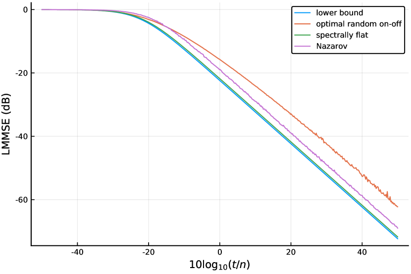
(a) i.i.d prior ($d(x)=\theta$ for $0\leq x\leq 1/2$)

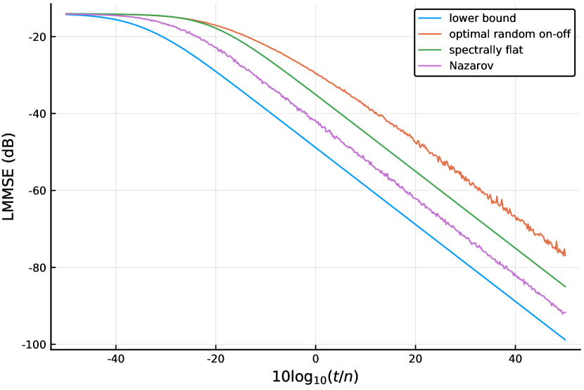
(b) bandlimited prior ($d(x)=\theta$ for $0\leq x\leq s-r$, $0$ for $x\geq s+r$, and $\theta(s+r-x)/(2r)$ otherwise for $0\leq x\leq 1/2$)

Fig. 1: $n=677,\theta=1,W=J=0.001,s=0.02,r=0.005$. We use the quartic residue construction for spectrally flat. Jaggedness of the Nazarov plot comes from the fact that in general the spectrum allocation varies with $t$ and we randomly seed the sign cortège.

4 Discussion and Future Work

Our refined analysis of a model drawing heavily from [14] yields tight conclusions across all scene correlation patterns and noise regimes, with sharp conclusions available in some specific scenarios. Moreover, we give heuristically efficient algorithms for the generation of optimal coded apertures. We also note that similar conclusions to our main results eqs. 3, 4 and 5 also hold for MI and Gaussian statistics of [14], simply because of the form of the expression for MI.

Furthermore, we note that our conclusions generalize naturally to 2D apertures, and in particular we have a tight characterization of optimal coded apertures in that setting. Concretely, one simply needs to take $\beta(n)^{2}$ as opposed to $\beta(n)$ due to the squaring of the $l_{1}$ lower bound for the 2D DFT. The rest of the analysis of Thm. 1 and Prop. 4 carries over naturally, with the orthogonal basis provided by products of $\psi_{j}$. We emphasize that this works regardless of the scene prior, even ones which are not separable. With an i.i.d. prior, separable apertures are optimal up to constants as in 1D, and in fact taking a product of spectrally flat apertures yields natural analogs of Props. 2, 3. However, with other priors, it seems like one needs the generality provided by Thm. 1. This work thus also answers the question of 2D apertures raised in [14]. We also view experimental verification of these ideas as a worthwhile task.

As noted in [14], [9] raises the question of whether continuous-valued masks perform better than binary-valued ones. This work sheds some light on this: the solution of Nazarov which we have shown is tight does seem to use the flexibility of the $l_{\infty}$ norm in an essential way; see, e.g., [32, p. 12] for more on this. And more specifically, we have numerical evidence for finite $n$; to give a concrete example, for $n=13$, the mask $[1,0,1,0,0,1,1,0,1,1,0,0,0]$ has optimal LMMSE for an i.i.d. scene over binary-valued masks for $\rho=6/13,\theta=0.01,W=J=0.001,t=130$, but is improved upon by the continuous-valued mask whose first entry is equal to $\epsilon$ and whose $i$th entry is equal to $1-\epsilon/6$ if $i-1$ is a quadratic residue modulo 13, and $0$ otherwise, for $0.26\leq\epsilon\leq 0.34$.

Although Prop. 4 shows universal tightness across all priors, even “extreme” ones like bandlimited ones, the constant is worse than that for a spectrally flat construction for i.i.d. scenes. The better performance of spectrally flat constructions over the ones inspired by Nazarov’s theorem seems to extend to other “natural” priors like the $f^{-\gamma}$ one, as the waterfilling still yields something that is nearly “flat”. It might be interesting to quantify and understand the “flatness” of the waterfilling for “natural” priors.

One issue that we have not addressed here or in [14] is the equal scaling of $n$ at both sensor and scene. One natural way to address this is letting $\mathbf{A}$ be $m\times n$, or alternatively one could study a continuous model. Another issue is obtaining a good understanding of mask/lens combinations. This will require not only updates to the simple propagation model studied here and in [14], but also a refined understanding of the cost tradeoffs between lenses and apertures.

Stepping back from imaging problems, one may ask the question of where else Nazarov’s theorem can be used in applied contexts, something also raised implicitly in [17]. For example, as Nazarov’s theorem does not care about orthogonality, but merely a $l_{2}$ estimate like Parseval’s theorem, one can use it for frames as well as bases, or for anything satisfying a restricted isometry property. Another example is the fact that we merely use the $l_{\infty}$ case of his theorem which works for all $l_{p}$ spaces.

5 Acknowledgement

Ganesh Ajjanagadde thanks Prof. Henry Cohn for discussions on pseudorandomness.

References

- [1] M Young, “Pinhole optics,” Applied Optics, vol. 10, no. 12, pp. 2763–2767, 1971.
- [2] JG Ables, “Fourier transform photography: a new method for x-ray astronomy,” Publications of the Astronomical Society of Australia, vol. 1, no. 4, pp. 172–173, 1968.
- [3] RH Dicke, “Scatter-hole cameras for x-rays and gamma rays,” The astrophysical journal, vol. 153, pp. L101, 1968.
- [4] Edward E Fenimore and Thomas M Cannon, “Coded aperture imaging with uniformly redundant arrays,” Applied optics, vol. 17, no. 3, pp. 337–347, 1978.
- [5] Adam Lloyd Cohen, “Anti-pinhole imaging,” Optica Acta: International Journal of Optics, vol. 29, no. 1, pp. 63–67, 1982.
- [6] Anat Levin, Rob Fergus, Frédo Durand, and William T Freeman, “Image and depth from a conventional camera with a coded aperture,” ACM transactions on graphics (TOG), vol. 26, no. 3, pp. 70, 2007.
- [7] Changyin Zhou, Stephen Lin, and Shree K Nayar, “Coded aperture pairs for depth from defocus and defocus deblurring,” International journal of computer vision, vol. 93, no. 1, pp. 53–72, 2011.
- [8] Ramesh Raskar, Amit Agrawal, and Jack Tumblin, “Coded exposure photography: motion deblurring using fluttered shutter,” ACM Transactions on Graphics (TOG), vol. 25, no. 3, pp. 795–804, 2006.
- [9] Ashok Veeraraghavan, Ramesh Raskar, Amit Agrawal, Ankit Mohan, and Jack Tumblin, “Dappled photography: Mask enhanced cameras for heterodyned light fields and coded aperture refocusing,” in ACM transactions on graphics (TOG). ACM, 2007, vol. 26, p. 69.
- [10] Marco F Duarte, Mark A Davenport, Dharmpal Takbar, Jason N Laska, Ting Sun, Kevin F Kelly, and Richard G Baraniuk, “Single-pixel imaging via compressive sampling,” IEEE signal processing magazine, vol. 25, no. 2, pp. 83–91, 2008.
- [11] M Salman Asif, Ali Ayremlou, Aswin Sankaranarayanan, Ashok Veeraraghavan, and Richard G Baraniuk, “Flatcam: Thin, lensless cameras using coded aperture and computation,” IEEE Transactions on Computational Imaging, vol. 3, no. 3, pp. 384–397, 2017.
- [12] Antonio Torralba and William T Freeman, “Accidental pinhole and pinspeck cameras: Revealing the scene outside the picture,” in Computer Vision and Pattern Recognition (CVPR), 2012 IEEE Conference on. IEEE, 2012, pp. 374–381.
- [13] Christos Thrampoulidis, Gal Shulkind, Feihu Xu, William T Freeman, Jeffrey H Shapiro, Antonio Torralba, Franco NC Wong, and Gregory W Wornell, “Exploiting occlusion in non-line-of-sight active imaging,” IEEE Transactions on Computational Imaging, vol. 4, no. 3, pp. 419–431, 2018.
- [14] Adam Yedidia, Christos Thrampoulidis, and Gregory Wornell, “Analysis and optimization of aperture design in computational imaging,” in 2018 IEEE International Conference on Acoustics, Speech and Signal Processing (ICASSP). IEEE, 2018, pp. 4029–4033.
- [15] RP Millane, S Alzaidi, and WH Hsiao, “Scaling and power spectra of natural images,” in Proc. Image and Vision Computing New Zealand, 2003, pp. 148–153.
- [16] Fedor L’vovich Nazarov, “The Bang solution of the coefficient problem,” Algebra i Analiz, vol. 9, no. 2, pp. 272–287, 1997, English translation in St. Petersburg Math. J. 9 (1998), no. 2, 407-419.
- [17] Holger Boche, Ezra Tampubolon, and W König, “Mathematics of signal design for communication systems,” in Mathematics and Society, pp. 185–220. European Mathematical Society Publishing House, 2016.
- [18] AJ Stam, “Some inequalities satisfied by the quantities of information of fisher and shannon,” Information and Control, vol. 2, no. 2, pp. 101–112, 1959.
- [19] Dongning Guo, Shlomo Shamai, and Sergio Verdú, “Mutual information and minimum mean-square error in Gaussian channels,” IEEE Transactions on Information Theory, vol. 51, no. 4, pp. 1261–1282, 2005.
- [20] Thøger Bang, “A solution of the“ plank problem”,” Proceedings of the American Mathematical Society, vol. 2, no. 6, pp. 990–993, 1951.
- [21] Karel De Leeuw, Yitzhak Katznelson, and Jean-Pierre Kahane, “Sur les coefficients de Fourier des fonctions continues,” CR Acad. Sci. Paris Sér. AB, vol. 285, no. 16, pp. A1001–A1003, 1977.
- [22] Keith Ball, “Convex geometry and functional analysis,” Handbook of the geometry of Banach spaces, vol. 1, pp. 161–194, 2001.
- [23] Yury Polyanskiy and Yihong Wu, “Lecture Notes on Information Theory,” http://people.lids.mit.edu/yp/homepage/data/itlectures_v5.pdf, 2018, [Online; accessed 21-September-2018].
- [24] Carl Friedrich Gauß, Disquisitiones Arithmeticae, Lipsiae In Commissis Apud Gerh. Fleischer Jux., 1801.
- [25] S Chowla, “A property of biquadratic residues,” Proc. Nat. Acad. Sci. India. Sect. A., vol. 14, pp. 45–46, 1944.
- [26] Emma Lehmer, “On residue difference sets,” Canad. J. Math, vol. 5, pp. 425–432, 1953.
- [27] Stefan Kohl (https://mathoverflow.net/users/28104/stefan-kohl), “Existence of polynomials of degree which represent infinitely many prime numbers,” https://mathoverflow.net/q/208614, [Online; accessed 02-October-2018].
- [28] Tom M Apostol, Introduction to analytic number theory, Springer Science & Business Media, 2013.
- [29] Terence Tao, “The Euler-Maclaurin formula, Bernoulli numbers, the zeta function, and real-variable analytic continuation,” https://tinyurl.com/ybweghs5, [Online; accessed 02-October-2018].
- [30] Daniel Spielman and Shang-Hua Teng, “Smoothed analysis of algorithms: Why the simplex algorithm usually takes polynomial time,” in Proceedings of the thirty-third annual ACM symposium on Theory of computing. ACM, 2001, pp. 296–305.
- [31] Omer Angel, Sébastien Bubeck, Yuval Peres, and Fan Wei, “Local max-cut in smoothed polynomial time,” in Proceedings of the 49th Annual ACM SIGACT Symposium on Theory of Computing. ACM, 2017, pp. 429–437.
- [32] Ben Green, “Spectral structure of sets of integers,” in Fourier analysis and convexity, pp. 83–96. Springer, 2004.