Generation of turbulence in colliding reconnection jets

Abstract

The collision of magnetic reconnection jets is studied by means of a three dimensional numerical simulation at kinetic scale, in the presence of a strong guide field. We show that turbulence develops due to the jets collision producing several current sheets in reconnection outflows, aligned with the guide field direction. The turbulence is mainly two-dimensional, with stronger gradients in the plane perpendicular to the guide field and a low wave-like activity in the parallel direction. First, we provide a numerical method to isolate the central turbulent region. Second, we analyze spatial second-order structure function and prove that turbulence is confined in this region. Finally, we compute local magnetic and electric frequency spectra, finding a trend in the sub-ion range that differs from typical cases for which the Taylor hypothesis is valid, as well as wave activity in the range between ion and electron cyclotron frequencies. Our results are relevant to understand observations of reconnection jets collisions in space plasmas.

1 Introduction

Magnetic reconnection is a fundamental phenomenon in astrophysical plasmas. It consists in the recombination of magnetic field topology due to the violation of the frozen-in law for magnetic field of ideal magnetohydrodinamics (MHD). Due to this recombination, plasma is ejected in the form of jets and magnetic energy is converted into kinetic energy. The presence of magnetic reconnection has been ascertained in the solar corona (Sui et al., 2004; Shibata, 1998), in the solar wind (Gosling, 2007; Phan et al., 2006; Retinò et al., 2007) and in the Earth’s magnetosphere (Burch et al., 2016), and it is thought to be responsible for particle acceleration and plasma heating in these environments (Drake et al., 2006). A close link exists between the presence of magnetic reconnection and the phenomenology of plasma turbulence (Matthaeus & Velli, 2011). In plasmas, similarly to fluid dynamics, magnetic and velocity fluctuation energy cascade from large to small scales, due to non-linear interactions, following the turbulent phenomenology. This non-linear cascade produces smaller and smaller scale magnetic shears, that can eventually undergo the process of magnetic reconnection. Magnetic reconnection, indeed, can be viewed as an active ingredient of plasma turbulence (Matthaeus & Lamkin, 1986; Servidio et al., 2009, 2011; Franci et al., 2017).

On the other hand, magnetic reconnection can act as a trigger of plasma turbulence in the reconnection outflows (Matthaeus & Lamkin, 1986; Malara et al., 1991, 1992; Lapenta, 2008; Huang & Bhattacharjee, 2010; Beresnyak, 2016). Numerical simulations have shown that reconnection outflows can comprise different types of plasma instabilities at both fluid (Guo et al., 2014) and kinetic scales (Vapirev et al., 2013; Huang et al., 2015). These instabilities, along with the presence of shears, make reconnection outflows turbulent rather than laminar. The latter is not just a numerical evidence, but has been recently confirmed by in situ spacecraft observations (Eastwood et al., 2009; Osman et al., 2015). Contrary to the “classical” view of reconnection energetics, where the conversion of magnetic into kinetic energy happens only in the main reconnection sites (Shay et al., 2007), reconnection outflows are now also believed to be regions where the plasma is heated and particles are accelerated (Daughton et al., 2011; Lapenta et al., 2014, 2015). It has been shown, both in numerical simulations (Leonardis et al., 2013; Pucci et al., 2017) and from most recent in-situ observation (Fu et al., 2017), that, due to turbulence, energy exchange between fields and particles in the outflows is intermittent. This means that the greatest part of energy transfer happens in low volume-filling, very intense current sheets. Recently, numerical simulations (Olshevsky et al., 2016) and observations (Fu et al., 2017) have shown that energy exchange is more efficient in the presence of magnetic null points of spiral topological type (O-point configurations) rather than the radial nulls (X-points). This suggests than energy dissipation is more efficient in a region surrounded by two, or multiple, X-lines. In the classical two-dimensional MHD picture of magnetic reconnection, an O-point is always present between the two X-points (for topological reasons), i.e., in the middle of two counter-propagating reconnection jets, if the X-lines are active.

The physics of reconnection jets collision has been studied numerically with both fluid and kinetic models (Karimabadi et al., 1999; Nakamura et al., 2010; Oka et al., 2008; Markidis et al., 2012), sometimes in the frame of the tearing or plasmoid instability (Bhattacharjee et al., 2009; Landi et al., 2015). Recently, the first observations of colliding reconnection jets have been carried out in the presence of both weak (Alexandrova et al., 2016) and strong (Øieroset et al., 2016) guide fields. Observational results show that jets collisions cause wave activity and are responsible for secondary reconnection events in the outflows, but a clear theoretical picture of reconnection jets collision is still lacking. In this work we present a three-dimensional (3D) numerical simulation to study the physics of reconnection jets collision, in the presence of a strong guide field, at kinetic scales. We show how jets collision gives rise to plasma turbulence in a confined region of the outflows. We provide a numerical method to detect the turbulent region and perform local statistical analysis to characterize the turbulence that is produced in such region. We believe that these results can be used for the interpretation of present and future observations of jets collisions at ion and sub-ion scales. Moreover, we provide a theoretical description of turbulence generated by magnetic reconnection in a three-dimensional kinetic model.

2 Numerical set up

We consider a plasma made of ions (protons) and electrons. At the initial time the plasma is at the Harris equilibrium

$${\bf B}=B_{0x}\tanh(y/\delta){\bf e_{x}}+B_{0z}{\bf e_{z}},\;\;n=n_{b}+\frac{n_{0}}{\cosh^{2}(y/\delta)},$$

where $B_{0z}$ is the guide field, $\delta$ is the thickness of the Harris sheet, and $n_{0b}$ the background density. The coordinates are chosen such that the equilibrium sheared magnetic field is directed along the $x$ axis, and varies along $y$, causing the initial current sheets to be directed parallel to the $z$ axis, which is also the guide field direction. For both species the initial distribution function is a Maxwellian with homogeneous temperature. The system obeys to the Vlasov-Maxwell equations, which are numerically solved using the semi-implicit particle-in-cell (PIC) code iPIC3D (Brackbill & Forslund, 1982; Markidis et al., 2010; Lapenta, 2012). The numerical domain is a Cartesian box with size $[40,\;30,\;10]\;d_{i}$, where $d_{i}$ is the ion inertial length. We use $[512,\;384,\;128]$ cells, each one initially populated with $125$ particles of each specie. A reduced ion/electron mass ratio $m_{i}/m_{e}=256$ is used, which fixes the spatial resolution to $\Delta x=1.25d_{e}$, where $d_{e}$ is the electron inertial length. The initial ion/electron temperature ratio is $T_{i}/T_{e}=5$, and thermal velocities $u_{th,i}=0.0063c$ and $u_{th,e}=0.045c$, where $c$ is the speed of light. The thickness of the initial current sheet is $\delta=0.5d_{i}$ and the background density is $n_{b0}/n_{0}=1/10$. The value of the guide field is set to $B_{0z}/B_{0x}=2$. We use open boundary condition in the $y$ direction and we impose periodicity along $x$ and $z$. The equilibrium is perturbed by a Gaussian fluctuation of the $z$ component of the vector potential, located at ($x=0,\;y=7.5$), which initializes the magnetic reconnection process (Lapenta et al., 2010). The system evolution is followed in time up to $29\tau_{i}$, where $\tau_{i}$ is the ion gyro-period, using a time step of $dt\approx\tau_{e}/10$, where $\tau_{e}$ is the electron gyro-period.

3 Dynamical evolution

Because of the strong guide field, we expect that current sheets will be preferentially aligned along the $z$ direction. In Figure 1, we represent a time evolution of the reconnecting current layer. The quantity plotted in panels (a-e) is $\langle J_{z}\rangle_{z}$, the out of plane total current density as a function of $x$ and $y$ and averaged along $z$. The initial Harris sheet is a narrow layer, directed along $z$, as reported in panel (a), and it has been perturbed at the boundary $x=0$. Because of periodicity, two reconnection sites form at opposite sides of the domain in the $x$ direction. Panel (f) shows the evolution of the mean square ion, electron and total current $\langle J^{2}\rangle$. At the beginning, the current is mainly carried by ions, due to the Harris equilibrium, but as the evolution proceeds electron current becomes dominant. The total current reaches a peak value at $84.06\Omega_{ci}^{-1}$ and rapidly decreases to a smaller value. Then, the value of $\langle J^{2}\rangle$ remains almost constant, slightly decreasing up to the end of the simulation.

The X-lines produce two reconnection jets which approach one against the other in the middle of the simulation domain (panel (b)). Notice that the two outflows carry oppositely directed current sheets even before the actual collision. When the two outflows collide, the maximum of $\langle J^{2}\rangle$ is reached (panel (c)). At that instant the two outflows can still be distinguished even though they look caught into each other. The two counter-propagating outflows carry with them also oppositely directed magnetic fields, which makes the system unstable to secondary reconnection. The large scale current sheets present in panel (c), whose dimension are of the order of $\sim 5-10d_{i}$, are fragmented in smaller ones by multiple reconnection events. The effect is visible in panel (d), where a multitude of current sheets at different scale appears in the collision region. This suggests the beginning of a turbulent cascade, that through nonlinear interactions forms smaller current sheets. At later times, the turbulence which develops in the center of the domain continuously generates and disrupts current sheets and the associated magnetic islands. It is worth noting that the area where the current sheets are located decreases in time (panel (e)). This is reasonable considering that the system is not driven externally, but is just relaxing after the jets collision.

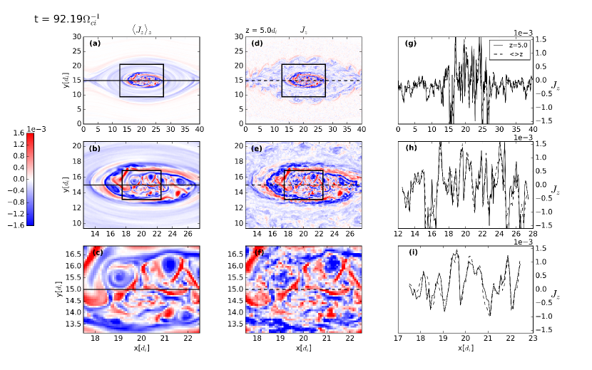
Figure 2: Telescopic view of $J_{z}$ at $t=92.19\Omega_{ci}^{-1}$. (a) Average out of plane current density $\langle J_{z}\rangle_{z}$ and two zooms (b)-(c). (d) Out of plane current density $J_{z}$ at $z=5.0d_{i}$ and two zooms (e)-(f). (g) Current density profile as a function of $x$, at $y=15.0d_{i}$, for $\langle J_{z}\rangle_{z}$ (solid line) and for $J_{z}(z=5.0)$ (dashed line) and two zooms (h)-(i). The black frames in panels (a)-(b) and (d)-(e) bound the zoomed regions showed in panels (b)-(c) and (e)-(f), respectively. The solid or dashed black lines in panels from (a) to (f) identify the locations along which the profiles in panels (g)-(h)-(i) are plotted.

We have just presented a 2D evolution of the system, relying on the fact that the presence of a strong magnetic field favors the formation of perpendicular gradients. To verify this assumption, in Figure 2 we present a comparison of $\langle J_{z}\rangle_{z}$ with $J_{z}$ at a fixed $z$, namely $z=5.0d_{i}$. The plot is taken in the turbulent phase at $t=92.19\Omega_{ci}^{-1}$ (panel (d) in Figure 1), right after the jets collision. $\langle J_{z}\rangle_{z}$ and $\langle J_{z}\rangle(z=5.0)$ in the $xy$ plane are plotted in the first and second column, respectively. The latter looks like the blurry version of the former. This can be interpreted as follows. The current sheets are elongated in the $z$ direction and, for this reason, they are not ruled out by the average. At the same time, a small level of fluctuation with wavevector in the $z$ direction are present, which make the picture of the 2D cut blurry. Those fluctuations are ruled out when averaging along $z$. In the third column a 1D cut of the two quantities is plotted as a function of $x$. We can see that several current sheets are encountered moving in the $x$ direction. The strongest ones are found in the central region. There is no big difference between the two variables, confirming that the fluctuations in the $z$ direction are small compared to the average current intensity. In the second and third row we show two zooms of the two quantities taken in the central part of the simulation. We observe that the two quantities look similar also at smaller scales. Moreover, we can notice that the size of the smallest current sheets are of a fraction ($1/5$ or less) of the ion inertial length $d_{i}$, corresponding to $\sim 3d_{e}$, where $d_{e}$ is the electron inertial length.

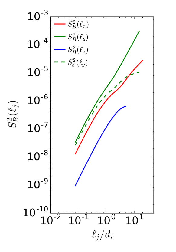
Figure 3: Second order structure function of the magnetic field $S^{2}_{B}$ at $t=92.19\Omega_{ci}^{-1}$ for lags in the $x$ (red), $y$ (green solid) and $z$ (blue) direction. The green dashed line represents the second order structure function of the magnetic field fluctuations $S^{2}_{b}$ along $y$ for which the background Harris field has been subtracted from the actual field.

This preliminary analysis has shown that a turbulent behavior is observed after the collision of the two jets. The comparison between $\langle J_{z}\rangle_{z}$ and $J_{z}(z=5.0)$ suggests that strong fluctuations are produced perpendicularly to the guide field, and small amplitude fluctuations are present along the guide field. In order to make the last statement more quantitative, we have analyzed the second order structure function of the magnetic field. This is defined as $S_{B}^{2}({\bf r})=\frac{1}{V}\int|{\bf B}({\bf x}+{\bf r})-{\bf B}({\bf x})|^{2}d^{3}x$, where ${\bf B}$ is the total magnetic field, ${\bf r}$ is a displacement in the physical space, and $V$ is the total volume of the simulation box. Similar to the power spectral density, this quantity represents the average of the magnetic fluctuations energy between two points of the domain separated by a lag ${\bf r}$. Since we are interested in evaluating the energy of the fluctuations varying in the direction parallel and perpendicular to $z$, i.e. the guide field direction, we have computed the so called reduced structure function defined as $S_{B}^{2}(\ell_{i})=\frac{1}{V}\int|{\bf B}({\bf x}+\ell_{i}{\bf e}_{i})-{\bf B}({\bf x})|^{2}d^{3}x$, with $i=x,y,z$. These quantities, plotted in Figure 3, represent the domain average of the magnetic energy fluctuations with wavevector in the $i$ direction at a scale $\ell$. For statistical reasons, we consider maximum lags $\ell_{i}^{max}=L_{j}/2$, where $L_{j}$ is the box size in the $j$ direction. The minimum lag is set to $\ell_{j}^{min}=\Delta x_{j}=1.25d_{e}$. The results confirm what suggested by the visual analysis of the current. The blue curve, representing $S_{B}^{2}(\ell_{z})$, is always below the red and green curves, representing $S_{B}^{2}(\ell_{x})$ and $S_{B}^{2}(\ell_{y})$, respectively. The magnetic fluctuation energy is larger for wavevector perpendicular to the guide field and smaller for parallel one at all scales. Moreover, the fluctuations in the direction of the initial shear, i.e. along $y$, are slightly stronger than the fluctuations in the $x$ direction. In order to check if this difference is due to the presence of the background Harris field we subtract its contribution to the total magnetic field, defining the new following variable: ${\bf b}={\bf B}-\langle{\bf B}_{x}(y)\rangle_{x,z}{\bf e}_{x}-B_{0z}{\bf e}_{z}$. The variable ${\bf b}$ can be seen as the magnetic fluctuation field. $S_{b}^{2}(\ell_{y})$ is plotted in Figure 3 as a green dashed line. The fluctuation energy in the $y$ direction are stronger than in the $x$ direction even when the contribution of the Harris field is not taken into account. Both are at least one order of magnitude stronger than the fluctuations in the $z$ direction. We can also notice that at large scales the structure function tends to saturate only in the $z$ direction. The saturation is reached at the scale of the correlation length. Since large scale shears are present in both the $x$ and $y$ direction, the corresponding structure function does not saturate for lags as large as half the box size in each direction. Consistently, when the contribution of the Harris field is subtracted from the total field, the structure function in the $y$ direction saturates at around $5d_{i}$. This size is comparable to the size of the turbulent region depicted in Figure 1 (panel (d)) and Figure 2.

The analysis of $S_{B}^{2}$ conducts to the result that turbulence develops in the box after jets collision. This turbulence is mainly two dimensional, with fluctuation energy concentrated in wavevectors perpendicular to the reconnection guide field. A second smaller anisotropy is found for the in plane fluctuations, where more energy is present in the direction of the initial magnetic shear. The analyses performed so far are global, in the sense that the full computational domain was used as a single sample. However, the turbulent region seems to be confined in a smaller central region surrounding the location where the outflows have collided. In the next section we provide a method to isolate that turbulent region and study its properties separately from the rest of the domain.

4 Isolating the turbulent region: method and local analysis

In this section we provide a method for isolating the turbulent region and we describe the turbulence analysis performed on the region itself comparing it with the rest of the simulation box.

4.1 The Method

In the previous section we have shown that turbulence develops in the simulated reconnection event, due to jets collision, and seems to be localized in the surrounding of the collision site. We have also shown that such turbulence is quasi two dimensional and develops in the plane perpendicular to the guide field. We build our method bearing on this last feature and considering the system as being two dimensional, thus neglecting the dependence on the $z$ component. In 2D MHD, the in-plane components of the magnetic field is a function only of the out-of-plane component of the vector potential ${\bf A}$. From ${\bf B}=\nabla\times{\bf A}$, one finds that $B_{x}=\frac{\partial A_{z}}{\partial y}$, and $B_{y}=-\frac{\partial A_{z}}{\partial x}$, where $xy$ is the 2D plane and $A_{z}$ is the $z$ component of ${\bf A}$. From the last two relations it is easy to show that $({\bf B}\cdot\nabla)A_{z}=0$. The last expression means that $A_{z}$ is constant moving along an in-plane field line or, equivalently, that in-plane magnetic field lines are isocontours of $A_{z}$. It is also easy to show that

$$-(\nabla\times{\bf B})_{z}=\nabla^{2}A_{z}.$$ (1)

This equation will be used later.

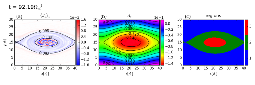
Figure 4: (a) Out of plane current averaged along z $\langle J_{z}\rangle_{z}$ and isocontours of the out of plane component of the vector potential $A_{z}$, (b) $A_{z}$ and its isocontours, (c) three regions: R1 (blue), R2 (green), R3 (red), as described in section 4.1.

Operationally, the two dimensional ingredient is obtained by averaging the magnetic field $\bf B$ in space, over the z direction. The z-average of the 2D magnetic field is similarly related to the z-average of the full 3D vector potential, that is the 2D potential $A_{z}=\hat{z}\cdot\langle{\bf A}\rangle_{z}$. This averaging operation has the effect of eliminating the fluctuations in the $z$ direction, which are however much smaller than those in $x$ and $y$, as shown previously. The map of the 2D potential $A_{z}$ is plotted in panel (b) of Figure 4, along with its isocontours, which are the in-plane magnetic field lines. In order to compute $A_{z}$, we solved Equation (1) using a Fourier method in an expanded (periodic) domain, then plotting the result in the original domain. The magnetic island produced by reconnection in the center of the box is clearly visible. Moreover, we notice that $A_{z}$ has a minimum in the middle of the island and a saddle point at the location of the main X-line. This is consistent with what found in incompressible MHD simulations of 2D magnetic reconnection (Matthaeus, 1982). It is also consistent with Equation (1), as we explain in the following. The presence of a minimum implies that $\nabla^{2}A_{z}>0$, and consequently $(\nabla\times{\bf B})_{z}<0$. From Maxwell equations, we know that $\nabla\times{\bf B}=\frac{1}{c}\frac{\partial{\bf E}}{\partial t}+\frac{4\pi}{c}{\bf J}$. At large scales and slow frequencies, the displacement current term can be neglected and the curl of ${\bf B}$ becomes proportional to ${\bf J}$. Considering that current in the initial current sheet is negative for construction, the minimum of $A_{z}$ in the middle of the island is justified. In panel (a) of Figure 4 we plot a 2D map of $\langle J_{z}\rangle_{z}$ at time $t=92.19\Omega_{ci}^{-1}$ and two isocontours of $A_{z}$, i.e. $A_{z}=-0.098$ and $A_{z}=-0.138$. The former represents the value of $A_{z}$ at the X-point and at the separatrices, the latter a manually selected value of $A_{z}$ associated with a magnetic field line enclosing most of the more turbulent central region and very little of the more quiescent (low current density) region surrounding it. These two isocontours identify three different regions, plotted in panel (c): Region 1 (R1), out the separatrices; Region 2 (R2), between the separatrices and the turbulent region; Region 3 (R3), the central turbulent region.

Since we want to reproduce such a distinction for each instant of time we have implemented the following numerical procedure. First, at a given time $t$ we compute the in-plane magnetic field average along $z$ and the corresponding 2D vector potential. Second, we find $A^{X}_{z}$, namely the value of $A_{z}$ at the X-point, and $A^{min}_{z}$, namely the minimum of $A_{z}$ located in the center of the domain. We call $A^{*}_{z}$ the suitable value of $A_{z}$ associated to the magnetic field line that encases the turbulent region. Since this value has to lay between $A^{min}_{z}$ and $A^{X}_{z}$, we can write it in this form:

$$A^{*}_{z}=A^{min}_{z}+a(A^{X}_{z}-A^{min}_{z}),{\mbox{with }}0<a<1.$$ (2)

Third, we find the suitable value of $a$ as that associated to a contour that encases all the strongest current sheets in the turbulent region. We found $a=1/6$ to be suitable for time $t=92.19\Omega_{ci}^{-1}$. Then, we repeat the procedure for each time step, keeping the selected value of $a$ unchanged. The procedure is applied from the time when the mean square current is maximum, i.e. $t=84.06\Omega_{ci}^{-1}$, up to the end of the simulation. Before that time it has no meaning separating the domain in regions, since turbulence has not developed yet. Choosing a fixed value for $a$ does not mean in principle that $A^{*}_{z}$ does not change in time, since both $A^{min}_{z}$ and $A^{X}_{z}$ can change. It rather means that we are choosing a value of the vector potential whose relative distance from the minimum and the value at the separatrices is constant. Interestingly, this choice gives a correct result for all time steps (see attached video). This can be explained considering that, from Maxwell’s equations, $\frac{\partial A_{z}}{\partial t}=-cE_{z}$, meaning that the value of $A_{z}$ changes due to the reconnection electric field. After the initial phase when jets are ejected, the value of this field become smaller causing the vector potential to be nearly constant in time on the separatrices. This method allows to identify different regions in the simulation domain in 2D. Since small fluctuations are present in the $z$ direction, we can extend the 2D region along $z$ and perform the statistical analysis on the 3D extension of each region.

4.2 The Analysis

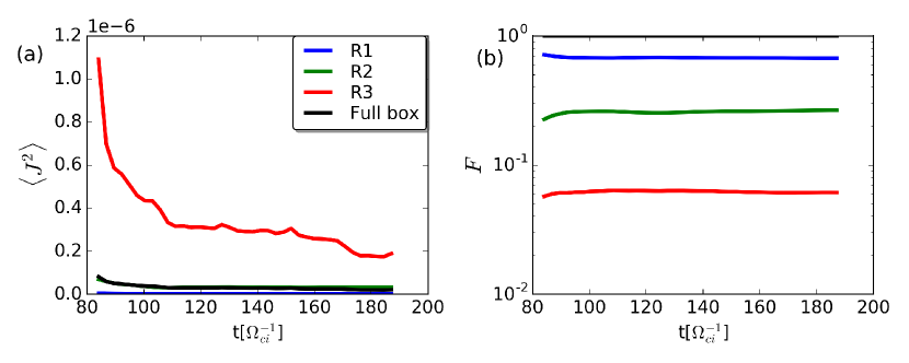
Figure 5: (a) Mean square current $\langle J^{2}\rangle$ as a function of time and (b) filling factor $F$ computed as the ratio between the volume of a region and the volume of the full box, for R1 (red), R2 (green), R3 (blue), and full box (black).

We have identified the turbulent region looking at the out of plane component of the total current, thus associating turbulence with the current activity. In Figure 5 we show the mean square current in the three regions R1, R2, and R3, as a function of time (panel (a)). The full box average is plotted as a reference. The mean square current in R3 is much higher than in R1 and R2. Its trend in time looks very similar to the trend of the full box average, shown in panel (f) of Figure 1. Panel (b) shows the filling factor $F$ of each region as a function of time, computed as the ratio between the volume of each region and the volume of the whole box. R3 is the smallest region and occupies around 6% of the total volume. The size of the region does not change significantly in time. This analysis shows that the most intense current sheets are within region R3, which is a small portion of the total domain. However, region R3 is large enough to perform a statistical analysis of fluctuations contained therein.

Since the chosen regions are not rectangular, and their boundaries are not periodic, a Fourier-based spectral analysis is not a suitable approach. For this reason, as done for the full box analysis, we compute the second order structure functions of the magnetic field in the three regions for lags in the $x$, $y$ or $z$ directions. In Figure 6 we report the result at time $t=92.19\Omega_{ci}^{-1}$. We notice first that the energy for parallel increment lags (panel (c)) is smaller than for perpendicular lags (panels (a) and (b)), in each region (panel (c)). Moreover, different regions have similar parallel fluctuations energy at all scales. Panels (a) and (b) show the second order structure function of the in-plane magnetic fluctuations. Due to the difference in shape and size of the regions, the curves do not span the same range of lags. The maximum possible lag is in fact defined as half of the sample size. The red curve, associated to region R3, terminates at smaller lags because it is obtained in the smallest region R3. Moreover, the maximum $\ell_{x}$ for R3 is bigger than the maximum $\ell_{y}$, since the shape of the region is elongated in the $x$ direction. At large scales, a saturation in the value of the second order structure function is observed just for R3. The lag at which the saturation is observed gives an estimate of the correlation length of around $5d_{i}$ along $x$ and $3d_{i}$ along $y$, which is comparable to the sizes of the region. Such saturation is not observed for R1 and R2, due to the presence of the large scale magnetic shear whose dimension is comparable to the sizes of those regions. At scales smaller than the correlation length, the red curve (R3) is always higher than green (R2) and blue (R1), $S^{2}_{B,R3}>S^{2}_{B,R2}>S^{2}_{B,R1}$.

The average energy of magnetic fluctuations varying in the plane perpendicular to the guide field is larger in R3, implying that the non-linear cascade has acted more efficiently in that region. Therefore, this proves that R3 is the actual region where turbulence develops.

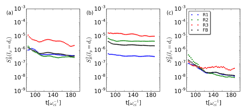
Figure 7: Second order structure functions of the magnetic field $S^{2}_{B}$ at $l_{i}=d_{i}$ as a function of time for $i$ equal to $x$ (a), $y$ (b) and $z$ (c). $S^{2}_{B}$ is computed in R1 (blue), R2 (green) and R3 (red), and in the full box (black).

In order to confirm that the turbulent cascade proceeds up to the end of the simulation, we have computed $S^{2}_{B}$ in each region for different times. At each time we take the value of $S^{2}_{B}$ for $\ell_{j}=d_{i}$ for $j=x,y,z$. The result is plotted in Figure 7. In the perpendicular directions the average of the magnetic fluctuation energy at scale $d_{i}$ is larger in R3, meaning that more energy is cascading to sub-ion scales in R3 compared to the rest of the domain. The energy in the $y$ direction is larger on average due to the presence of the Harris field. In the $z$ direction the values in R3 become eventually larger as the simulation proceeds. At earlier times, the large energy is R2 is due to the formation of an electron instability that develops on the separatrices (Daughton et al., 2011; Fermo et al., 2012). This instability remains confined in R2 and saturates for times larger than $t\sim 100\Omega_{ci}^{-1}$.

To complete our analysis, we study the Eulerian frequency spectra of the electric and magnetic field in R3. The fields have been sampled during the simulation at a cadence of $3\Delta t$ by means of probes (‘virtual satellites’) placed at predefined locations inside the simulation box. For the analysis we present here, we have used satellites from a region of dimensions $1.25\times 1.25\times 10.0\;d^{3}_{i}$ located in the middle of R3. The selected region contains $3\times 3\times 24=216$ equally spaced satellites. We analyze the data in the time frame $92.18\Omega_{ci}^{-1}<t<187.09\Omega_{ci}^{-1}$, extending from the initial development of the turbulence to the end of the simulation. Similar to what happens for in-situ spacecraft observations, magnetic field data are not periodic. Moreover, the situation we are considering here is not stationary, since turbulence in R3 is decaying in time. In order to avoid spurious effects coming from signal detrending or windowing, we use the technique proposed by Bieber et al. (1993) to compute the frequency power spectra. This method has been used, e.g., for the analysis of the recent in situ solar wind observations (Bale et al., 2005). The method follows these steps. First, the series of the increments is computed from the actual field. If B(t) is the magnetic field as a function of time, its increments are defined as: $\Delta{\bf B}(t)={\bf B}(t+\Delta t)-{\bf B}(t)$. Second, the autocorrelation function of the increments is computed as $R^{(\Delta)}_{ii}(\tau)=\frac{1}{V}\int\Delta{\bf B}_{i}(t)\Delta{\bf B}_{i}(t+\tau)dt$. Third, from the autocorrelation function the power spectrum from the increments $P^{(\Delta)}_{ii}(f)$ is computed via Fourier transform. Finally, the spectrum of the actual field $P_{ii}(f)$ is recovered by filtering the spectrum of the increments:

$$P_{ii}(f)=\frac{P^{(\Delta)}_{ii}(f)}{4\sin^{2}(\pi/\Delta t)}.$$

This procedure suppresses the contribution of the low frequencies unresolved in the chosen sample. Computing power spectral density from autocorrelation function can yield to non-physical results such as negative power spectrum values (Blackman & Tukey, 1958), therefore we limit our analysis to lags smaller than $\tau_{max}=T/10$, where $T$ is the duration of the total sample. With this upper limit we have enough statistics to estimate the spectrum for all frequencies selected.

Figure 8, reports the power spectra of magnetic (panel (a)) and electric (panel (b)) field as a function of frequency. The spectra are computed for each probe separately and then averaged. In Figure 8 both spectra of the three components and total field are plotted. Characteristic frequencies are marked by vertical lines. Reference lines are shown correspnding to spectral indices of $-3$ and $-1$. The computed spectra span frequency ranges that extend from a fraction of the ion cyclotron frequency to beyond the electron cyclotron frequency. The electron plasma frequency is poorly resolved. Note that the range of plotted frequencies doesn’t reach the Nyquist frequency because the fields are saved each $3\Delta t$. Magnetic and electric frequency spectra from fluid to electron scales in plasma turbulence have been recently studied by means of in-situ spacecraft observations in the magnetosheath by Matteini et al. (2017). It has been shown that the magnetic and electric spectra have approximately similar behavior in the fluid-MHD like regime, while they show different trends in the kinetic range. In particular, the magnetic field spectrum steepens at ion scales, passing from a spectral index between $-5/3$ and $-3/2$ in the MHD fluid range to a roughly $-3$ spectral index at ion and sub-ion scale. The electric field has an opposite trend, passing from a spectral index $-3/2$ in the fluid range to roughly $-1$ in the kinetic range. The familiar theoretical explanation for this phenomenon (e.g., Matthaeus et al. (2008)) depends on dominance in the kinetic range of non-ideal terms in the generalized Ohm’s law. When the turbulence $\bf k$-vectors are mainly perpendicular to the guide field, this heuristic explanation predicts $\delta E^{2}\propto k^{2}\delta B^{2}$ for an electromagnetic fluctuation at a given wavevector $k$ in the sub-ion range.

The above reasoning explains the relationship of observed frequency and wavenumber spectra in cases in which the two are proportional and related by the Taylor hypothesis, appropriate for high speed super-Alfvénic flows. This explains the agreement of frequency spectra coming from single spaceraft observations (Bale et al., 2005; Eastwood et al., 2009; Matteini et al., 2017), with wavenumber spectra obtained from numerical simulations (Pucci et al., 2017; Franci et al., 2017).

The results we report here seem to be, at a first sight, in contrast to the above scenario, in that the sub-ion scale magnetic and electric spectra in our analysis do not follow a specific power law and strongly differ from a $\propto f^{-3}$ and a $\propto f^{-1}$ trend, respectively. The main reason for this apparent discrepancy relies on the fact that Taylor hypothesis is not valid in the system considered here, as we presently demonstrate.

The Taylor hypothesis consists in assuming that time variations at a single observational point are only due to the rapid sweeping of spatial structure past that point. This requires that the large scale bulk flow of the plasma greatly exceeds all characteristic dynamical speeds that might distort those structures. This includes both wave propagation and turbulent velocity (Perri et al., 2017). When Taylor hypothesis is not verified, there is not a simple connection between the frequency and wavenumber spectra, although there remains the possibility of a statistical similarity between the Eulerian frequency spectra and the wavenumber spectra (Chen & Kraichnan, 1989; Matthaeus & Bieber, 1999) when the dominant effect is random large scale sweeping.

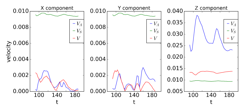
Figure 9: Characteristic speeds in the probes region. $V_{s}$, $\bf{V_{a}}$ and $\bf{V}$ are the average ion sound speed, the average Alfvén velocity and the average bulk velocity, respectively. The three panels show the $x$ (left), $y$ (middle), and $z$ (right) components of the velocities and the ion sound speed.

The Taylor hypothesis in not valid in the system we are considering here. In order to assess this hypothesis, the bulk velocity of the plasma, computed in the region where the virtual satellites are located, must be compared with characteristic wave speeds and with turbulent velocity fluctuations. In Figure 9 we report the comparison between the bulk velocity ${\bf V}$, the Alfvén velocity ${\bf V}_{A}$, and the ion sound speed $V_{s}$. The bulk velocity ${\bf V}$ is defined as the plasma center of mass velocity, the Aflvén velocity as ${\bf V_{A}}={\bf B}/\sqrt{4\pi\rho}$, where $\rho$ is the ion density, and the ion sound speed as $V_{S}=\sqrt{\frac{\gamma\sum_{j}P_{jj}}{3\rho}}$, where $j=(x,y,z)$, $P$ is the ion pressure tensor, and $\gamma$ is the adiabatic index, which we have chosen equal to $5/3$ for simplicity. These characteristic macroscopic speeds are compared in Figure 9, which shows the $x$, $y$ and $z$ components of ${\bf V}$ and ${\bf V}_{A}$, and the the ion sound speed (considered isotropic). The bulk speed is in every case smaller or comparable with the other two characteristic speeds. In particular, the ion sound speed is the larger speed in the directions perpendicular to the guide field, while the Alfvén speed is, as expected, the largest speed in the parallel direction.

Next the bulk speed is compared with measures of the turbulent fluctuation velocities in Figure 10. In particular we compute the longitudinal increments ${u}({\bf r},{\bf\ell})=\hat{{\bf\ell}}\cdot[{\bf V}({\bf r}+{\bf\ell})-{\bf V}({\bf r})]$, where ${\bf r}$ is a position in space, and ${\bf\ell}$ is the direction along which the velocity increments are computed. The root mean square velocity increments are computed in terms of components along the three Cartesian directions as $u_{rms}(\ell_{i})=\sqrt{\langle{\bf u}({\bf r},{\bf\ell_{i}})\cdot{\bf u}({\bf r},{\bf\ell_{i}})\rangle}$. Here $\langle\rangle$ means average in the region where the probe are located, and $\ell_{i}$ with $i=x,y,z$ indicates the direction along which the velocity increments are computed. We considered a lag size equal to $d_{i}$ for each direction. In this way, we examine in particular whether the Taylor hypothesis is valid for the kinetic features seen in the frequency spectra in Figure 8. Figure 10 shows a comparison of the bulk velocity with these measures of fluctuations. Each panel contains the i-th component of the bulk velocity and the corresponding $u_{rms}(\ell_{i})$. First, we notice that $u_{rms}(\ell_{z})$ is smaller than $u_{rms}(\ell_{x})$, and $u_{rms}(\ell_{y})$, in accordance with anisotropic, quasi 2D turbulence developed in the plane perpendicular to the guide field. Second, we notice that $V_{z}$ the bulk speed along the guide field direction is larger than all $u_{rms}$. This large speed could in principle be responsible for a similarity between the $k_{z}$ spectrum and the frequency spectrum. However, as shown in the previous section, turbulence is mainly 2D due to the presence of the strong guide field, and very little energy is contained in the $k_{z}$ modes. Moreover, the largest characteristic speed in the $z$ direction is the Alfvén speed (see panel (c) in Figure 9), which allows for the presence of fast parallel propagating waves of Alfvènic nature that can invalidate the Taylor hypothesis.

Based on this analysis of characteristic speeds, we can conclude that the Taylor hypothesis is not verified in the location where the Eulerian spectra are computed. Therefore a similarity between frequency and wavenumber spectra is not expected. The magnetic and electric frequency spectra presented in Figure 8 are therefore to be considered as independent of the spatial (wavenumber) structure. Then the observed features are essentially temporal, and the observed features indicate the presence of wave activity at different temporal scales, which we now briefly describe.

First, we notice a flattening of the magnetic spectrum between the ion and electron cyclotron frequency, around $f=10^{-1}$, relative to the $\propto f^{-3}$ trend at lower frequencies. This feature is consistent with the presence of whistler waves and is also found in in-situ observations (Matteini et al., 2017). To confirm this hypothesis, we applied a pass band filter at a frequency $f_{ce}/5$ to the magnetic field (not shown here) finding a phase shift between $B_{x}$ and $B_{y}$ consistent with parallel propagating whistler.

Second, a significant peak at the electron cyclotron frequency is observed in both electric and magnetic field spectra. The peak is found for all the three components of the fields probably indicating the presence of both electromagnetic and electrostatic modes. To verify that this peak is not due to a numerical artifact, we ran a new simulation (not shown) with an halved time step and saving the fields data at each computational cycle. No relevant change in the results was observed, either in the peak intensity or in its position in frequency. Therefore we conclude that the peak is associated with physical electron cyclotron modes.

It is worth noticing how the aforementioned presence of wave modes at different time scales in not in contrast with a picture of fully developed turbulence. Previous MHD studies have proven that Eulerian frequency spectra can present intensity peaks at fixed frequencies associated to wave modes even when no signature of such modes is present in the wavenumber spectra (Dmitruk et al., 2004; Dmitruk & Matthaeus, 2009). A result similar to the one presented here was found recently in two dimensional hybrid simulations of kinetic plasma turbulence, where several peaks at frequency larger than the ion cyclotron frequencies have been found in the Eulerian spectra of the magnetic field (Parashar et al., 2010). Here we show such a behavior in a turbulent environment that is self-consistently generated by magnetic reconnection. A detailed description of the modes that contribute to shape the frequency spectra along with the effects due to the lack of validity of Taylor hypothesis goes beyond the scope of this work and will be considered for future studies.

5 Discussion and conclusion

We presented a full kinetic 3D simulation of reconnection in the presence of a strong guide field with reduced mass ratio. The simulation considered periodic boundary conditions in the direction of the outflow allowing counter propagating reconnection jets to collide. We showed that the collision of reconnection jets coming from two neighbouring X-lines drives turbulence in the magnetic island within them. Turbulence manifests in the continuous disruption and formation of new currents sheets mainly directed along the guide field, whose thicknesses range between the electron and ion inertial lengths.

The turbulence produced in the collision is quasi two dimensional, with stronger gradients in the direction pependicular to the guide field. Dynamical activity in the electric current density remains well confined in a small region of the simulation box that occupies a small percentage (6%) of the total volume. Using an idenitification method based on the the magnetic vector potential, we numerically separated the turbulent region from the rest of the computational domain. Analysis of spacial second order structure functions show that the selected central region is where turbulence actually develops allowing an efficient cascade of magnetic energy to sub-ion scales. This cascade remains active for the duration of our simulation. Since there is no forcing except for the initial one due to jets collision, the current activity slightly reduces in time, remaining confined in the same region.

Power spectrum analysis of electric and magnetic fluctuations in the turbulent region reveal interesting properties that, at first sight, stand in contrast to a number of previous observations and numerical simulations. However, the assumption of Taylor hypothesis made in previous works do not apply to this case, which explains the apparent discrepancy. Under these conditions, the Eulerian frequency spectra computed in our analysis are quite independent of the spectra computed in the Taylor hypothesis scenario, which are interpreted as wavenumber spectra. There is no simple relationship between spatial structure and temporal structure in the present case. Interestingly, the analysis of Eulerian frequency spectra in the turbulent region reveals the presence of wave activity at different frequencies: parallel propagating whistler between the ion and electron cyclotron frequency, and electromagnetic and electrostatic modes at the electron cyclotron frequencies. The presence of whistlers in the region compressed by counter streaming reconnection jets was recently found in in-situ observation in the case of small guide field (Alexandrova et al., 2016). Electrostatic and electromagnetic wave activity at the electron cyclotron frequency has been also detected in previous observations of magnetic reconnection in the vicinity of the reconnection sites (Tang et al., 2013; Viberg et al., 2013; Khotyaintsev et al., 2016). Here, we observed electron cyclotron wave activity in the turbulent region formed by reconnection jets collision.

In a recent paper, Øieroset et al. (2016) have shown the first observation of reconnection jets collision in the presence of a strong guide field. The dynamical picture presented in that work imagined an event of secondary reconnection activated by the counter propagating jets both carrying magnetic field lines with opposite polarities. Our simulation shows that the physical situation can be less laminar than predicted and that turbulence develops after jets collision producing several current sheets, secondary reconnection events, and wave modes up to the electron cyclotron frequency. Our results strongly agrees with the recent results by Fu et al. (2017), which have found turbulent magnetic reconnection in the region surrounding an O-point. The present results are likely to be relevant for the interpretation of future observations of collisions of reconnection jets, which may have distinctive signatures in space and astrophysical plasmas.

Figure 1: (a-e) $J_{z}$ averaged along z at different times. (f) Mean square ion (blue), electron (red), and total (black) current as a function of time. Dashed lines in panel (f) indicate plotting times of panels (a)-(e).

Figure 6: Second order structure functions of the magnetic field $S^{2}_{B}$ at $t=92.19\Omega_{ci}^{-1}$ for lags $\ell$ along $x$ (a), $y$ (b) and $z$ (c). $S^{2}_{B}$ is computed in R1 (blue), R2 (green) and R3 (red), and in the full box (black).

Figure 8: Power spectrum of magnetic (a) and electric (b) fluctuations for $x$ (blue), $y$ (green) and $z$ (red) component, and for the total field (light-blue). The black dashed lines represent a power law of the type $\propto f^{-3}$ in panel (a) and of the type $\propto f^{-1}$ in panel (b). In both panels vertical lines on the $x$ axis represent: ion cyclotron frequency $f_{ci}$, lower-hybrid frequency $f_{lh}$, ion plasma frequency $f_{pi}$, electron cyclotron frequency $f_{ce}$, electron plasma frequency $f_{pe}$, and the Nyquist frequency $1/2\Delta t$, computed and averaged in the region where the probes are located.

Figure 10: Comparison of bulk speed with turbulent velocity at scale $d_{i}$. The three panel show the $x$ (left), $y$ (middle) and $z$ (right) components of the velocities. The bulk speed components are plotted in black, while red dashed curves represent the turbulent velocity computed considering lags directed along $x$, $y$, and $z$, respectively.

Appendix A Appendix information

References

- Alexandrova et al. (2016) Alexandrova, A., Nakamura, R., Panov, E. V., et al. 2016, Geophysical Research Letters, 43, 7795
- Bale et al. (2005) Bale, S., Kellogg, P., Mozer, F., Horbury, T., & Reme, H. 2005, Physical Review Letters, 94, 215002
- Beresnyak (2016) Beresnyak, A. 2016, The Astrophysical Journal, 834, 47
- Bhattacharjee et al. (2009) Bhattacharjee, A., Huang, Y.-M., Yang, H., & Rogers, B. 2009, Physics of Plasmas (1994-present), 16, 112102
- Bieber et al. (1993) Bieber, J. W., Chen, J., Matthaeus, W. H., Smith, C. W., & Pomerantz, M. A. 1993, Journal of Geophysical Research: Space Physics, 98, 3585
- Blackman & Tukey (1958) Blackman, R. B., & Tukey, J. W. 1958
- Brackbill & Forslund (1982) Brackbill, J., & Forslund, D. 1982, Journal of Computational Physics, 46, 271
- Burch et al. (2016) Burch, J., Torbert, R., Phan, T., et al. 2016, Science, 352, aaf2939
- Chen & Kraichnan (1989) Chen, S., & Kraichnan, R. H. 1989, Physics of Fluids A: Fluid Dynamics, 1, 2019
- Daughton et al. (2011) Daughton, W., Roytershteyn, V., Karimabadi, H., et al. 2011, Nature Physics, 7, 539
- Dmitruk & Matthaeus (2009) Dmitruk, P., & Matthaeus, W. 2009, Physics of Plasmas, 16, 062304
- Dmitruk et al. (2004) Dmitruk, P., Matthaeus, W. H., & Lanzerotti, L. J. 2004, Geophysical research letters, 31
- Drake et al. (2006) Drake, J., Swisdak, M., Che, H., & Shay, M. 2006, Nature, 443, 553
- Eastwood et al. (2009) Eastwood, J., Phan, T., Bale, S., & Tjulin, A. 2009, Physical review letters, 102, 035001
- Fermo et al. (2012) Fermo, R., Drake, J., & Swisdak, M. 2012, Physical review letters, 108, 255005
- Franci et al. (2017) Franci, L., Cerri, S. S., Califano, F., et al. 2017, The Astrophysical Journal Letters, 850, L16
- Fu et al. (2017) Fu, H., Vaivads, A., Khotyaintsev, Y. V., et al. 2017, Geophysical Research Letters, 44, 37
- Gosling (2007) Gosling, J. 2007, The Astrophysical Journal Letters, 671, L73
- Guo et al. (2014) Guo, L.-J., Huang, Y.-M., Bhattacharjee, A., & Innes, D. E. 2014, The Astrophysical Journal Letters, 796, L29
- Huang et al. (2015) Huang, C., Lu, Q., Guo, F., et al. 2015, Geophysical Research Letters, 42, 7282
- Huang & Bhattacharjee (2010) Huang, Y.-M., & Bhattacharjee, A. 2010, Physics of Plasmas (1994-present), 17, 062104
- Karimabadi et al. (1999) Karimabadi, H., Krauss-Varban, D., Omidi, N., & Vu, H. 1999, Journal of Geophysical Research: Space Physics, 104, 12313
- Khotyaintsev et al. (2016) Khotyaintsev, Y. V., Graham, D., Norgren, C., et al. 2016, Geophysical Research Letters, 43, 5571
- Landi et al. (2015) Landi, S., Del Zanna, L., Papini, E., Pucci, F., & Velli, M. 2015, The Astrophysical Journal, 806, 131
- Lapenta (2008) Lapenta, G. 2008, Physical review letters, 100, 235001
- Lapenta (2012) —. 2012, Journal of Computational Physics, 231, 795
- Lapenta et al. (2014) Lapenta, G., Goldman, M., Newman, D., Markidis, S., & Divin, A. 2014, Physics of Plasmas (1994-present), 21, 055702
- Lapenta et al. (2010) Lapenta, G., Markidis, S., Divin, A., Goldman, M., & Newman, D. 2010, Physics of Plasmas, 17, 082106
- Lapenta et al. (2015) Lapenta, G., Markidis, S., Goldman, M. V., & Newman, D. L. 2015, Nature Physics, 11, 690
- Leonardis et al. (2013) Leonardis, E., Chapman, S. C., Daughton, W., Roytershteyn, V., & Karimabadi, H. 2013, Physical review letters, 110, 205002
- Malara et al. (1991) Malara, F., Veltri, P., & Carbone, V. 1991, Physics of Fluids B: Plasma Physics (1989-1993), 3, 1801
- Malara et al. (1992) —. 1992, Physics of Fluids B: Plasma Physics (1989-1993), 4, 3070
- Markidis et al. (2012) Markidis, S., Henri, P., Lapenta, G., et al. 2012, Nonlinear Processes in Geophysics, 19, 145
- Markidis et al. (2010) Markidis, S., Lapenta, G., & Rizwan-uddin. 2010, Mathematics and Computers in Simulation, 80, 1509
- Matteini et al. (2017) Matteini, L., Alexandrova, O., Chen, C. H. K., & Lacombe, C. 2017, Monthly Notices of the Royal Astronomical Society, 466, 945
- Matthaeus & Bieber (1999) Matthaeus, W., & Bieber, J. 1999in , AIP, 515–518
- Matthaeus & Lamkin (1986) Matthaeus, W., & Lamkin, S. L. 1986, Physics of Fluids (1958-1988), 29, 2513
- Matthaeus & Velli (2011) Matthaeus, W., & Velli, M. 2011, Space science reviews, 160, 145
- Matthaeus (1982) Matthaeus, W. H. 1982, Geophysical Research Letters, 9, 660
- Matthaeus et al. (2008) Matthaeus, W. H., Servidio, S., & Dmitruk, P. 2008, 101, 149501
- Nakamura et al. (2010) Nakamura, T., Fujimoto, M., & Sekiya, H. 2010, Geophysical Research Letters, 37
- Øieroset et al. (2016) Øieroset, M., Phan, T., Haggerty, C., et al. 2016, Geophysical Research Letters, 43, 5536
- Oka et al. (2008) Oka, M., Fujimoto, M., Nakamura, T., Shinohara, I., & Nishikawa, K.-I. 2008, Physical review letters, 101, 205004
- Olshevsky et al. (2016) Olshevsky, V., Deca, J., Divin, A., et al. 2016, The Astrophysical Journal, 819, 52
- Osman et al. (2015) Osman, K., Kiyani, K., Matthaeus, W., et al. 2015, The Astrophysical Journal Letters, 815, L24
- Parashar et al. (2010) Parashar, T., Servidio, S., Breech, B., Shay, M., & Matthaeus, W. 2010, Physics of Plasmas, 17, 102304
- Perri et al. (2017) Perri, S., Servidio, S., Vaivads, A., & Valentini, F. 2017, The Astrophysical Journal Supplement Series, 231, 4
- Phan et al. (2006) Phan, T., Gosling, J., Davis, M., et al. 2006, Nature, 439, 175
- Pucci et al. (2017) Pucci, F., Servidio, S., Sorriso-Valvo, L., et al. 2017, The Astrophysical Journal, 841, 60
- Retinò et al. (2007) Retinò, A., Sundkvist, D., Vaivads, A., et al. 2007, Nature Physics, 3, 236
- Servidio et al. (2009) Servidio, S., Matthaeus, W., Shay, M., Cassak, P., & Dmitruk, P. 2009, Physical review letters, 102, 115003
- Servidio et al. (2011) Servidio, S., Dmitruk, P., Greco, A., et al. 2011, Nonlinear Processes in Geophysics, 18, 675
- Shay et al. (2007) Shay, M., Drake, J., & Swisdak, M. 2007, Physical review letters, 99, 155002
- Shibata (1998) Shibata, K. 1998, Astrophysics and Space Science, 264, 129
- Sui et al. (2004) Sui, L., Holman, G. D., & Dennis, B. R. 2004, The Astrophysical Journal, 612, 546
- Tang et al. (2013) Tang, X., Cattell, C., Dombeck, J., et al. 2013, Geophysical Research Letters, 40, 2884
- Vapirev et al. (2013) Vapirev, A., Lapenta, G., Divin, A., et al. 2013, Journal of Geophysical Research: Space Physics, 118, 1435
- Viberg et al. (2013) Viberg, H., Khotyaintsev, Y. V., Vaivads, A., André, M., & Pickett, J. 2013, Geophysical Research Letters, 40, 1032