Abstract

We investigate how to train kernel approximation methods that generalize well under a memory budget. Building on recent theoretical work, we define a measure of kernel approximation error which we find to be more predictive of the empirical generalization performance of kernel approximation methods than conventional metrics. An important consequence of this definition is that a kernel approximation matrix must be high rank to attain close approximation. Because storing a high-rank approximation is memory intensive, we propose using a low-precision quantization of random Fourier features (LP-RFFs) to build a high-rank approximation under a memory budget. Theoretically, we show quantization has a negligible effect on generalization performance in important settings. Empirically, we demonstrate across four benchmark datasets that LP-RFFs can match the performance of full-precision RFFs and the Nyström method, with 3x-10x and 50x-460x less memory, respectively.

1 INTRODUCTION

Kernel methods are a powerful family of machine learning methods. A key technique for scaling kernel methods is to construct feature representations whose inner products approximate the kernel function, and then learn a linear model with these features; important examples of this technique include the Nyström method (Williams and Seeger, 2000) and random Fourier features (RFFs) (Rahimi and Recht, 2007). Unfortunately, a large number of features are typically needed for attaining strong generalization performance with these methods on big datasets (Rahimi and Recht, 2008; Tu et al., 2016; May et al., 2017). Thus, the memory required to store these features can become the training bottleneck for kernel approximation models. In this paper we work to alleviate this memory bottleneck by optimizing the generalization performance for these methods under a fixed memory budget.

To gain insight into how to design more memory-efficient kernel approximation methods, we first investigate the generalization performance vs. memory utilization of Nyström and RFFs. While prior work (Yang et al., 2012) has shown that the Nyström method generalizes better than RFFs under the the same number of features, we demonstrate that the opposite is true under a memory budget. Strikingly, we observe that $50,000$ standard RFFs can achieve the same heldout accuracy as $20,000$ Nyström features with 10x less memory on the TIMIT classification task. Furthermore, this cannot be easily explained by the Frobenius or spectral norms of the kernel approximation error matrices of these methods, even though these norms are the most common metrics for evaluating kernel approximation methods (Gittens and Mahoney, 2016; Yang et al., 2014; Sutherland and Schneider, 2015; Yu et al., 2016; Dao et al., 2017); the above Nyström features attain 1.7x smaller Frobenius error and 17x smaller spectral error compared to the RFFs. This observation suggests the need for a more refined measure of kernel approximation error—one which better aligns with generalization performance, and can thus better guide the design of new approximation methods.

Table 1: Memory utilization for kernel approximation methods. We consider data $x\in\mathbb{R}^{d}$, kernel features $z(x)\in\mathbb{R}^{m}$, mini-batch size $s$, # of classes $c$ (for regression/binary classification $c=1$). We assume full-precision numbers are 32 bits. We measure a method’s memory utilization as the sum of the three components in this table.

Approximation Method	Feature generation	Feature mini-batch	Model parameters
Nyström	$32(md+m^{2})$	$32ms$	$32mc$
RFFs	$32md$	$32ms$	$32mc$
Circulant RFFs	$32m$	$32ms$	$32mc$
Low-precision RFFs, $b$ bits (ours)	$32m$	$bms$	$32mc$

Building on recent theoretical work (Avron et al., 2017), we define a measure of approximation error which we find to be much more predictive of empirical generalization performance than the conventional metrics. In particular, we extend Avron et al.’s definition of $\Delta$-spectral approximation to our definition of $(\Delta_{1},\Delta_{2})$-spectral approximation by decoupling the two roles played by $\Delta$ in the original definition. This decoupling reveals that $\Delta_{1}$ and $\Delta_{2}$ impact generalization differently, and can together much better explain the relative generalization performance of Nyström and RFFs than the original $\Delta$, or the Frobenius or spectral errors. This $(\Delta_{1},\Delta_{2})$ definition has an important consequence—in order for an approximate kernel matrix to be close to the exact kernel matrix, it is necessary for it to be high rank.

Motivated by the above connection between rank and generalization performance, we propose using low-precision random Fourier features (LP-RFFs) to attain a high-rank approximation under a memory budget. Specifically, we store each random Fourier feature in a low-precision fixed-point representation, thus achieving a higher-rank approximation with more features in the same amount of space. Theoretically, we show that when the quantization noise is much smaller than the regularization parameter, using low precision has negligible effect on the number of features required for the approximate kernel matrix to be a $(\Delta_{1},\Delta_{2})$-spectral approximation of the exact kernel matrix. Empirically, we demonstrate across four benchmark datasets (TIMIT, YearPred, CovType, Census) that in the mini-batch training setting, LP-RFFs can match the performance of full-precision RFFs (FP-RFFs) as well as the Nyström method, with 3x-10x and 50x-460x less memory, respectively. These results suggest that LP-RFFs could be an important tool going forward for scaling kernel methods to larger and more challenging tasks.

The rest of this paper is organized as follows: In Section 2 we compare the performance of the Nyström method and RFFs in terms of their training memory footprint. In Section 3 we present a more refined measure of kernel approximation error to explain the relative performance of Nyström and RFFs. We introduce the LP-RFF method and corresponding analysis in Section 4, and present LP-RFF experiments in Section 5. We review related work in Section 6, and conclude in Section 7.

2 NYSTRÖM VS. RFFS: AN EMPIRICAL COMPARISON

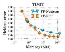
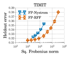
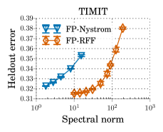
(a)	(b)	(c)	(d)

Figure 1: Generalization performance of full-precision RFFs and Nyström with respect to the number of features and training memory footprint on TIMIT (a,b). Nyström performs better for a fixed number of features, while RFFs perform better under a memory budget. We also see that the generalization performance of these methods does not align well with the Frobenius or spectral norms of their respective kernel approximation error matrices (c,d). For results on YearPred, CovType, and Census, see Appendix D.2.

To inform our design of memory-efficient kernel approximation methods, we first perform an empirical study of the generalization performance vs. memory utilization of Nyström and RFFs. We begin by reviewing the memory utilization for these kernel approximation methods in the mini-batch training setting; this is a standard setting for training large-scale kernel approximation models (Huang et al., 2014; Yang et al., 2015; May et al., 2017), and it is the setting we will be using to evaluate the different approximation methods (Sections 2.2, 5.1). We then show that RFFs outperform Nyström given the same training memory budget, even though the opposite is true given a budget for the number of features (Yang et al., 2012). Lastly, we demonstrate that the Frobenius and spectral norms of the kernel approximation error matrix align poorly with generalization performance, suggesting the need for a more refined measure of approximation error for evaluating the quality of a kernel approximation method; we investigate this in Section 3.

For background on RFFs and the Nyström method, and for a summary of our notation, see Appendix A.

2.1 Memory Utilization

The optimization setting we consider is mini-batch training over kernel approximation features. To understand the training memory footprint, we present in Table 1 the memory utilization of the different parts of the training pipeline. The three components are:

1. Feature generation: Computing $m$ RFFs over data in $\mathbb{R}^{d}$ requires a random projection matrix $W\in\mathbb{R}^{m\times d}$. The Nyström method stores $m$ “landmark points” $\hat{x}_{i}\in\mathbb{R}^{d}$, and a projection matrix in $\mathbb{R}^{m\times m}$.

2. Feature mini-batch: Kernel approximation features $z(x_{i})\in\mathbb{R}^{m}$ for all $x_{i}$ in a mini-batch are stored.

3. Model parameters: For binary classification and regression, the linear model learned on the $z(x)$ features is a vector $\theta\in\mathbb{R}^{m}$; for $c$-class classification, it is a matrix $\theta\in\mathbb{R}^{m\times c}$.

In this work we focus on reducing the memory occupied by the mini-batches of features, which can occupy a significant fraction of the training memory. Our work is thus orthogonal to existing work which has shown how to reduce the memory utilization of the feature generation (Le et al., 2013; Yu et al., 2015) and the model parameters (Sainath et al., 2013a; Sindhwani et al., 2015; De Sa et al., 2018) (e.g., using structured matrices or low precision). Throughout this paper, we measure the memory utilization of a kernel approximation method as the sum of the above three components.

2.2 Empirical Comparison

We now compare the generalization performance of RFFs and the Nyström method in terms of their training memory footprint. We demonstrate that RFFs can outperform the Nyström method given a memory budget, and show that the difference in performance between these methods cannot be explained by the Frobenius or spectral norms of their kernel approximation error matrices.

In experiments across four datasets (TIMIT, YearPred, CovType, Census (Garofolo et al., 1993; Dheeru and Karra Taniskidou, 2017)), we use up to 20k Nyström features and 400k RFFs to approximate the Gaussian kernel; we train the models using mini-batch stochastic gradient descent with early stopping, with a mini-batch size of 250. We present results averaged from three random seeds, with error bars indicating standard deviations (for further experiment details, see Appendix D.2). In Figure 1(a) we observe that as a function of the number of kernel approximation features the Nyström method generally outperforms RFFs, though the gap narrows as $m$ approaches 20k. However, we see in Figure 1(b) that RFFs attain better generalization performance as a function of memory. Interestingly, the relative performance of these methods cannot simply be explained by the Frobenius or spectral norms of the kernel approximation error matrices; in Figure 1(c,d) we see that there are many cases in which the RFFs attain better generalization performance, in spite of having larger Frobenius or spectral approximation error. This is a phenomenon we observe on other datasets as well (Appendix D.2). This suggests the need for a more refined measure of the approximation error of a kernel approximation method, which we discuss in the following section.

3 A REFINED MEASURE OF KERNEL APPROX. ERROR

To explain the important differences in performance between Nyström and RFFs, we define a more refined measure of kernel approximation error—$(\Delta_{1},\Delta_{2})$-spectral approximation. Our definition is an extension of Avron et al.’s definition of $\Delta$-spectral approximation, in which we decouple the two roles played by $\Delta$ in the original definition. This decoupling allows for a more fine-grained understanding of the factors influencing the generalization performance of kernel approximation methods, both theoretically and empirically. Theoretically, we present a generalization bound for kernel approximation methods in terms of $(\Delta_{1},\Delta_{2})$ (Sec. 3.1), and show that $\Delta_{1}$ and $\Delta_{2}$ influence the bound in different ways (Prop. 1). Empirically, we show that $\Delta_{1}$ and $\Delta_{2}$ are more predictive of the Nyström vs. RFF performance than the $\Delta$ from the original definition, and the Frobenius and spectral norms of the kernel approximation error matrix (Sec. 3.2, Figure 2). An important consequence of the $(\Delta_{1},\Delta_{2})$ definition is that attaining a small $\Delta_{1}$ requires a large number of features; we leverage this insight to motivate our proposed method, low-precision random Fourier features, in Section 4.

3.1 $(\Delta_{1},\Delta_{2})$-spectral Approximation

We begin by reviewing what it means for a matrix $A$ to be a $\Delta$-spectral approximation of a matrix $B$ (Avron et al., 2017). We then extend this definition to $(\Delta_{1},\Delta_{2})$-spectral approximation, and bound the generalization performance of kernel approximation methods in terms of $\Delta_{1}$ and $\Delta_{2}$ in the context of fixed design kernel ridge regression.

Definition 1.

For $\Delta\geq 0$, a symmetric matrix $A$ is a $\Delta$-spectral approximation of another symmetric matrix $B$ if $(1-\Delta)B\preceq A\preceq(1+\Delta)B$.

We extend this definition by allowing for different values of $\Delta$ in the left and right inequalities above:

Definition 2.

For $\Delta_{1},\Delta_{2}\geq 0$, a symmetric matrix $A$ is a $(\Delta_{1},\Delta_{2})$-spectral approximation of another symmetric matrix $B$ if $(1-\Delta_{1})B\preceq A\preceq(1+\Delta_{2})B$.

Throughout the text, we will use $\Delta$ to denote the variable in Def. 1, and $(\Delta_{1},\Delta_{2})$ to denote the variables in Def. 2. In our discussions and experiments, we always consider the smallest $\Delta$, $\Delta_{1}$, $\Delta_{2}$ satisfying the above definitions; thus, $\Delta=\max(\Delta_{1},\Delta_{2})$.

In the paragraphs that follow we present generalization bounds for kernel approximation models in terms of $\Delta_{1}$ and $\Delta_{2}$ in the context of fixed design kernel ridge regression, and demonstrate that $\Delta_{1}$ and $\Delta_{2}$ influence generalization in different ways (Prop. 1). We consider the fixed design setting because its expected generalization error has a closed-form expression, which allows us to analyze generalization performance in a fine-grained fashion. For an overview of fixed design kernel ridge regression, see Appendix A.3.

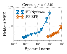
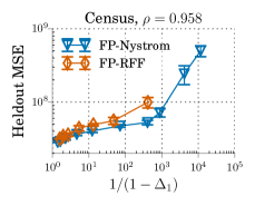
Figure 2: The correlation between generalization performance and different measures of kernel approximation error for the full-precision RFF and Nyström methods. We see that generalization performance aligns well with $1/(1-\Delta_{1})$ (Spearman rank correlation coefficient $\rho=0.958$), while aligning poorly with $\Delta$ and the spectral and squared Frobenius norms of the kernel approximation error matrix. See Appendix D.3 for results on CovType.

In the fixed design setting, given a kernel matrix $K\in\mathbb{R}^{n\times n}$, a regularization parameter $\lambda\geq 0$, and a set of labeled points $\{(x_{i},y_{i})\}_{i=1}^{n}$ where the observed labels $y_{i}=\bar{y}_{i}+\epsilon_{i}$ are randomly perturbed versions of the true labels $\bar{y}_{i}\in\mathbb{R}$ ($\epsilon_{i}$ independent, $\mathbb{E}\left[\epsilon_{i}\right]=0$, $\mathbb{E}\left[\epsilon_{i}^{2}\right]=\sigma^{2}<\infty$), it is easy to show (Alaoui and Mahoney, 2015) that the optimal kernel regressor $f_{K}$ has expected error

$$\mathcal{R}(f_{K})=\frac{\lambda^{2}}{n}\bar{y}^{T}(K+\lambda I)^{-2}\bar{y}+\frac{\sigma^{2}}{n}\mathop{\rm tr}\Big{(}K^{2}(K+\lambda I)^{-2}\Big{)},$$

where $\bar{y}=(\bar{y}_{1},\ldots,\bar{y}_{n})$ is the vector of true labels.

This closed-form expression for generalization error allows us to bound the expected loss $\mathcal{R}(f_{\tilde{K}})$ of a kernel ridge regression model $f_{\tilde{K}}$ learned using an approximate kernel matrix $\tilde{K}$ in place of the exact kernel matrix $K$. In particular, if we define

$$\widehat{\mathcal{R}}(f_{K}) :=\frac{\lambda}{n}\bar{y}^{T}(K+\lambda I)^{-1}\bar{y}+\frac{\sigma^{2}}{n}\mathop{\rm tr}\Big{(}K(K+\lambda I)^{-1}\Big{)},$$

which is an upper bound on $\mathcal{R}(f_{K})$, we can bound the expected loss of $f_{\tilde{K}}$ as follows:

Proposition 1.

(Extended from (Avron et al., 2017)) Suppose $\tilde{K}+\lambda I$ is $(\Delta_{1},\Delta_{2})$-spectral approximation of $K+\lambda I$, for $\Delta_{1}\in[0,1)$ and $\Delta_{2}\geq 0$. Let $m$ denote the rank of $\tilde{K}$, and let $f_{K}$ and $f_{\tilde{K}}$ be the kernel ridge regression estimators learned using these matrices, with regularizing constant $\lambda\geq 0$ and label noise variance $\sigma^{2}<\infty$. Then

$$\mathcal{R}(f_{\tilde{K}})\leq\frac{1}{1-\Delta_{1}}\widehat{\mathcal{R}}(f_{K})+\frac{\Delta_{2}}{1+\Delta_{2}}\frac{m}{n}\sigma^{2}.$$ (1)

We include a proof in Appendix B.1. This result shows that smaller values for $\Delta_{1}$ and $\Delta_{2}$ imply tighter bounds on the generalization performance of the model trained with $\tilde{K}$. We can see that as $\Delta_{1}$ approaches 1 the bound diverges, and as $\Delta_{2}$ approaches $\infty$ the bound plateaus. We leverage this generalization bound to understand the difference in performance between Nyström and RFFs (Sec. 3.2), and to motivate and analyze our proposed low-precision random Fourier features (Sec. 4).

Remark

The generalization bound in Prop. 1 assumes the regressor $f_{K}$ is computed via the closed-form solution for kernel ridge regression. However, in Sections 4-5 we focus on stochastic gradient descent (SGD) training for kernel approximation models. Because SGD can also find the model which minimizes the regularized empirical loss (Nemirovski et al., 2009), the generalization results carry over to our setting.

3.2 Revisiting Nyström vs. RFF Comparison

In this section we show that the values of $\Delta_{1}$ and $\Delta_{2}$ such that the approximate kernel matrix is a $(\Delta_{1},\Delta_{2})$-spectral approximation of the exact kernel matrix correlate better with generalization performance than the original $\Delta$, and the Frobenius and spectral norms of the kernel approximation error; we measure correlation using Spearman’s rank correlation coefficient $\rho$.

To study the correlation of these metrics with generalization performance, we train Nyström and RFF models for many feature dimensions on the Census regression task, and on a subsampled version of 20k train and heldout points from the CovType classification task. We choose these small datasets to be able to compute the various measures of kernel approximation error over the entire heldout set. We measure the spectral and Frobenius norms of $K-\tilde{K}$, and the $\Delta$ and $(\Delta_{1},\Delta_{2})$ values between $K+\lambda I$ and $\tilde{K}+\lambda I$ ($\lambda$ chosen via cross-validation), where $K$ and $\tilde{K}$ are the exact and approximate kernel matrices for the heldout set. For more details about these experiments and how we compute $\Delta$ and $(\Delta_{1},\Delta_{2})$, see Appendix D.3.

In Figure 2, we plot the generalization performance on these tasks as a function of these metrics; while the original $\Delta$ and the Frobenius and spectral norms generally do not align well with generalization performance, we see that $\frac{1}{1-\Delta_{1}}$ does. Specifically, $\frac{1}{1-\Delta_{1}}$ attains a Spearman rank correlation coefficient of $\rho=0.958$, while squared Frobenius norm, spectral norm, and the original $\Delta$ attain values of 0.594, 0.540, and 0.759. In Appendix D.3 we show these trends are robust to different kernel approximation methods and datasets. For example, we show that while other approximation methods (e.g., orthogonal RFFs (Yu et al., 2016)), like Nyström, can attain much lower Frobenius and spectral error than standard RFFs, this does not translate to improved $\Delta_{1}$ or heldout performance. These results mirror the generalization bound in Proposition 1, which grows linearly with $\frac{1}{1-\Delta_{1}}$. For simplicity, we ignore the role of $\Delta_{2}$ here, as $\Delta_{1}$ appears to be sufficient for explaining the main differences in performance between these full-precision methods. In Sections 4.2 and 5.2, however, we show that $\Delta_{2}$ has a large influence on generalization performance for low-precision features.

Now that we have seen that $\Delta_{1}$ has significant theoretical and empirical impact on generalization performance, it is natural to ask how to construct kernel approximation matrices that attain small $\Delta_{1}$. An important consequence of the definition of $\Delta_{1}$ is that for $\tilde{K}+\lambda I$ to have small $\Delta_{1}$ relative to $K+\lambda I$, $\tilde{K}$ must be high-rank; in particular, a necessary condition is $\Delta_{1}\geq\frac{\lambda_{m+1}(K)}{\lambda_{m+1}(K)+\lambda}$, where $m$ is the rank of $\tilde{K}$ and $\lambda_{i}(K)$ is the $i^{th}$ largest eigenvalue of $K$. This sets a lower bound on the rank necessary for $\tilde{K}$ to attain small $\Delta_{1}$ which holds regardless of the approximation method used, motivating us to design high-rank kernel approximation methods.

4 LOW-PRECISION RANDOM FOURIER FEATURES (LP-RFFS)

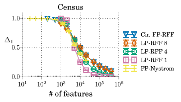
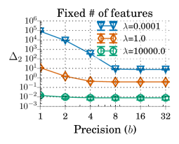
Figure 3: Empirical validation of Theorem 2. In the left and middle plots (shared legend), we see that as the # of features grows, LP-RFFs approach $\Delta_{1}=0$, but plateau at larger $\Delta_{2}$ values (at most $\delta_{b}^{2}/\lambda$, marked by dashed lines) for very low precisions. In the right plot we see that the larger $\lambda$ is, the lower the precision at which using low precision does not impact $\Delta_{2}$. For $\Delta_{1}$ and $\Delta_{2}$ vs. # features plots on CovType, see Appendix D.4.

Taking inspiration from the above-mentioned connection between the rank of the kernel approximation matrix and generalization performance, we propose low-precision random Fourier features (LP-RFFs) to create a high-rank approximation matrix under a memory budget. In particular, we quantize each random Fourier feature to a low-precision fixed-point representation, thus allowing us to store more features in the same amount of space. Theoretically, we show that when the quantization noise is small relative to the regularization parameter, using low precision has minimal impact on the number of features required for the approximate kernel matrix to be a $(\Delta_{1},\Delta_{2})$-spectral approximation of the exact kernel matrix; by Proposition 1, this implies a bound on the generalization performance of the model trained on the low-precision features. At the end of this section (Section 4.3), we discuss a memory-efficient implementation for training a full-precision model on top of LP-RFFs.

4.1 Method Details

The core idea behind LP-RFFs is to use $b$ bits to store each RFF, instead of $32$ or $64$ bits. We implement this with a simple stochastic rounding scheme. We use the parametrization $z_{i}(x)=\sqrt{2/m}\cos(w_{i}^{T}x+a_{i})\in[-\sqrt{2/m},\sqrt{2/m}]$ for the RFF vector $z(x)\in\mathbb{R}^{m}$ (Rahimi and Recht, 2007), and divide this interval into $2^{b}-1$ sub-intervals of equal size $r=\frac{2\sqrt{2/m}}{2^{b}-1}$. We then randomly round each feature $z_{i}(x)$ to either the top or bottom of the sub-interval $[\underline{z},\overline{z}]$ containing it, in such a way that the expected value is equal to $z_{i}(x)$; specifically, we round $z_{i}(x)$ to $\underline{z}$ with probability $\frac{\overline{z}-z}{\overline{z}-\underline{z}}$ and to $\overline{z}$ with probability $\frac{z-\underline{z}}{\overline{z}-\underline{z}}$. The variance of this stochastic rounding scheme is at most $\delta_{b}^{2}/m$, where $\delta_{b}^{2}:=2/(2^{b}-1)^{2}$ (Prop. 7 in App. C.2). For each low-precision feature $\tilde{z}_{i}(x)$ we only need to store the integer $j\in[0,2^{b}-1]$ such that $\tilde{z}_{i}(x)=-\sqrt{2/m}+jr$, which takes $b$ bits. Letting $\tilde{Z}\in\mathbb{R}^{n\times m}$ denote the matrix of quantized features, we call $\tilde{K}=\tilde{Z}\tilde{Z}^{T}$ an $m$-feature $b$-bit LP-RFF approximation of a kernel matrix $K$.

As a way to further reduce the memory footprint during training, we leverage existing work on using circulant random matrices (Yu et al., 2015) for the RFF random projection matrix to only occupy $32m$ bits. All our LP-RFF experiments use circulant projections.

4.2 Theoretical Results

In this section we show quantization has minimal impact on the number of features required to guarantee strong generalization performance in certain settings. We do this in the following theorem by lower bounding the probability that $\tilde{K}+\lambda I$ is a $(\Delta_{1},\Delta_{2})$-spectral approximation of $K+\lambda I$, for the LP-RFF approximation $\tilde{K}$ using $m$ features and $b$ bits per feature.

Theorem 2.

Let $\tilde{K}$ be an $m$-feature $b$-bit LP-RFF approximation of a kernel matrix $K$, assume $\|K\|\geq\lambda\geq\delta^{2}_{b}:=2/(2^{b}-1)^{2}$, and define $a:=8\mathop{\rm tr}\left((K+\lambda I_{n})^{-1}(K+\delta^{2}_{b}I_{n})\right)$. Then for any $\Delta_{1}\geq 0$, $\Delta_{2}\geq\delta^{2}_{b}/\lambda$,

$$\mathbb{P}\Big{[}{\textstyle(1-\Delta_{1})(K+\lambda I)\preceq\tilde{K}+\lambda I\preceq(1+\Delta_{2})(K+\lambda I)}\Big{]}\geq$$

$${1\!-\!a\!\left(\!\!\exp\!\left(\!\frac{-m\Delta_{1}^{2}}{\frac{4n}{\lambda}(1+\frac{2}{3}\Delta_{1})}\right)\!+\!\exp\!\left(\frac{-m(\Delta_{2}-\frac{\delta^{2}_{b}}{\lambda})^{2}}{\frac{4n}{\lambda}(1+\frac{2}{3}(\Delta_{2}-\frac{\delta^{2}_{b}}{\lambda}))}\!\right)\!\!\right)}.$$

The proof of Theorem 2 is in Appendix C. To provide more intuition we present the following corollary:

Corollary 2.1.

Assuming $\Delta_{1}\leq 3/2$, it follows that $(1-\Delta_{1})(K\!+\!\lambda I_{n})\preceq\tilde{K}+\lambda I_{n}$ with probability at least $1-\rho$ if $m\geq\frac{8n/\lambda}{\Delta_{1}^{2}}\log\Big{(}\frac{a}{\rho}\Big{)}.$ Similarly, assuming $\Delta_{2}\in\big{[}\frac{\delta_{b}^{2}}{\lambda},\frac{3}{2}\big{]}$, it follows that $\tilde{K}+\lambda I_{n}\preceq(1+\Delta_{2})(K+\lambda I_{n})$ with probability at least $1-\rho$ if $m\geq\frac{8n/\lambda}{(\Delta_{2}-\delta_{b}^{2}/\lambda)^{2}}\log\Big{(}\frac{a}{\rho}\Big{)}.$

The above corollary suggests that using low precision has negligible effect on the number of features necessary to attain a certain value of $\Delta_{1}$, and also has negligible effect for $\Delta_{2}$ as long as $\delta_{b}^{2}/\lambda\ll\Delta_{2}$.

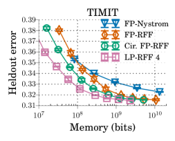
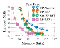
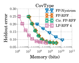
Figure 4: Generalization performance of FP-Nyström, FP-RFFs, circulant FP-RFFs, and LP-RFFs with respect to memory (sum of components in Table 1) on TIMIT, YearPred and CovType. LP-RFFs attain the best performance across a wide range of memory budgets. The same trend holds for Census in Appendix D.5.

Validation of Theory

We now empirically validate the following two predictions made by the above theory: (1) Using low precision has no effect on the asymptotic behavior of $\Delta_{1}$ as the number of features $m$ approaches infinity, while having a significant effect on $\Delta_{2}$ when $\delta_{b}^{2}/\lambda$ is large. Specifically, as $m\rightarrow\infty$, $\Delta_{1}$ converges to 0 for any precision $b$, while $\Delta_{2}$ converges to a value upper bounded by $\delta_{b}^{2}/\lambda$. (2) If $\delta_{b}^{2}/\lambda\ll\Delta_{2}$, using $b$-bit precision will have negligible effect on the number of features required to attain this $\Delta_{2}$. Thus, the larger $\lambda$ is, the smaller the impact of using low precision should be on $\Delta_{2}$.

To validate the first prediction, in Figure 3 (left, middle) we plot $\Delta_{1}$ and $\Delta_{2}$ as a function of the number of features $m$, for FP-RFFs and LP-RFFs; we use the same $\lambda$ as in the Section 2 Census experiments. We show that for large $m$, all methods approach $\Delta_{1}=0$; in contrast, for precisions $b\leq 4$ the LP-RFFs converge to a $\Delta_{2}$ value much larger than 0, and slightly less than $\delta_{b}^{2}/\lambda$ (marked by dashed lines).

To validate the second prediction, in Figure 3 (right) we plot $\Delta_{2}$ vs. precision for various values of $\lambda$, using $m=2000$ features for all precisions; we do this on a random subsample of 8000 Census training points. We see that for large enough precision $b$, the $\Delta_{2}$ is very similar to the value from using 32-bit precision. Furthermore, the larger the value of $\lambda$, the smaller the precision $b$ can be without significantly affecting $\Delta_{2}$.

4.3 Implementation Considerations

In this paper, we focus on training full-precision models using mini-batch training over low-precision features. Here we describe how this mixed-precision optimization can be implemented in a memory-efficient manner.

Naively, to multiply the low-precision features with the full-precision model, one could first cast the features to full-precision, requiring significant intermediate memory. We can avoid this by casting in the processor registers. Specifically, to perform multiplication with the full-precision model, the features can be streamed to the processor registers in low precision, and then cast to full precision in the registers. In this way, only the features in the registers exist in full precision. A similar technique can be applied to avoid intermediate memory in the low-precision feature computation—after a full-precision feature is computed in the registers, it can be directly quantized in-place before it is written back to main memory. We leave a more thorough investigation of these systems issues for future work.

Table 2: The compression ratios achieved by LP-RFFs relative to the best performing full-precision baselines.

	FP-RFFs	Cir. FP-RFFs	Nyström
Census	2.9x	15.6x	63.2x
YearPred	10.3x	7.6x	461.6x
Covtype	4.7x	3.9x	237.2x
TIMIT	5.1x	2.4x	50.9x

5 EXPERIMENTS

In this section, we empirically demonstrate the performance of LP-RFFs under a memory budget, and show that $(\Delta_{1},\Delta_{2})$ are predictive of generalization performance. We show in Section 5.1 that LP-RFFs can attain the same performance as FP-RFFs and Nyström, while using 3x-10x and 50x-460x less memory. In Section 5.2, we show the strong alignment between $(\Delta_{1},\Delta_{2})$ and generalization performance, once again validating the importance of this measure.

5.1 Empirical Evaluation of LP-RFFs

To empirically demonstrate the generalization performance of LP-RFFs, we compare their performance to FP-RFFs, circulant FP-RFFs, and Nyström features for various memory budgets. We use the same datasets and protocol as the large-scale Nyström vs. RFF comparisons in Section 2.2; the only significant additions here are that we also evaluate the performance of circulant FP-RFFs, and LP-RFFs for precisions $b\in\{1,2,4,8,16\}$. Across our experiments, we compute the total memory utilization as the sum of all the components in Table 1. We note that all our low-precision experiments are done in simulation, which means we store the quantized values as full-precision floating-point numbers. We report average results from three random seeds, with error bars showing standard deviations. For more details about our experiments, see Appendix D.5. We use the above protocol to validate the following claims on the performance of LP-RFFs.

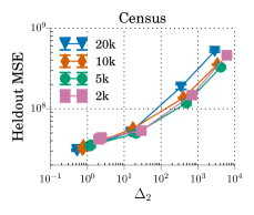
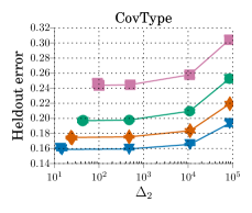
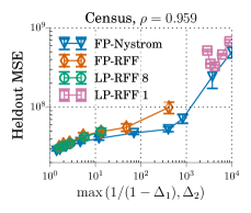
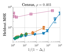
Figure 5: Generalization perf. vs. $\Delta_{2}$ (left plots, shared legend), and vs. $1/(1-\Delta_{1})$ and $\max\left(1/(1-\Delta_{1}),\Delta_{2}\right)$ (right plots, shared legend). Left: heldout performance deteriorates as $\Delta_{2}$ gets larger due to lower precision. Right: $\max\left(1/(1-\Delta_{1}),\Delta_{2}\right)$ aligns well with performance across LP-RFF precisions (Spearman rank correlation coefficient $\rho=0.959$), while $1/(1-\Delta_{1})$ aligns poorly ($\rho=0.403$). See Appendix D.6 for CovType results.

LP-RFFs can outperform full-precision features under memory budgets.

In Figure 4, we plot the generalization performance for these experiments as a function of the total training memory for TIMIT, YearPred, and CovType. We observe that LP-RFFs attain better generalization performance than the full-precision baselines under various memory budgets. To see results for all precisions, as well as results on additional benchmark datasets (Census, Adult, Cod-RNA, CPU, Forest) from the UCI repository (Dheeru and Karra Taniskidou, 2017), see Appendix D.5.

LP-RFFs can match the performance of full-precision features with significantly less memory.

In Table 2 we present the compression ratios we achieve with LP-RFFs relative to the best performing baseline methods. For each baseline (FP-RFFs, circulant FP-RFFs, Nyström), we find the smallest LP-RFF model, as well as the smallest baseline model, which attain within $10^{-4}$ relative performance of the best-performing baseline model; we then compute the ratio of the memory used by these two models (baseline/LP-RFF) for three random seeds, and report the average. We can see that LP-RFFs demonstrate significant memory saving over FP-RFFs, circulant FP-RFFs, and Nyström, attaining compression ratios of 2.9x-10.3x, 2.4x-15.6x, and 50.9x-461.6x, respectively.

5.2 Generalization Performance vs. $(\Delta_{1},\Delta_{2})$

In this section we show that $\Delta_{1}$ and $\Delta_{2}$ are together quite predictive of generalization performance across all the kernel approximation methods we have discussed. We first show that performance deteriorates for larger $\Delta_{2}$ values as we vary the precision of the LP-RFFs, when keeping the number of features constant (thereby limiting the influence of $\Delta_{1}$ on performance). We then combine this insight with our previous observation (Section 3.2) that performance scales with $\frac{1}{1-\Delta_{1}}$ in the full-precision setting by showing that across precisions the performance aligns well with $\max\big{(}\frac{1}{1-\Delta_{1}},\Delta_{2}\big{)}$. For these experiments, we use the same protocol as for the $(\Delta_{1},\Delta_{2})$ experiments in Section 3.2, but additionally consider LP-RFFs for precisions $b\in\{1,2,4,8,16\}$.

We show in Figure 5 (left plots) that for a fixed number of random Fourier features, performance deteriorates as $\Delta_{2}$ grows. As we have shown in Figure 3 (left), $\Delta_{1}$ is primarily governed by the rank of the approximation matrix, and thus holding the number of features constant serves as a proxy for holding $\Delta_{1}$ roughly constant. This allows us to isolate the impact of $\Delta_{2}$ on performance as we vary the precision.

To integrate the influence of $\Delta_{1}$ and $\Delta_{2}$ on generalization performance into a single scalar, we consider $\max\big{(}\frac{1}{1-\Delta_{1}},\Delta_{2}\big{)}$. In Figure 5 (right plots) we show that when considering both low-precision and full-precision features, $\max\big{(}\frac{1}{1-\Delta_{1}},\Delta_{2}\big{)}$ aligns well with performance ($\rho=0.959$, incorporating all precisions), while $\frac{1}{1-\Delta_{1}}$ aligns poorly ($\rho=0.403$).

In Appendix B we argue that performance scales roughly as $\Delta_{2}$ instead of as $\Delta_{2}/(1+\Delta_{2})$ (as suggested by Prop. 1) due to looseness in the Prop. 1 bound.

6 RELATED WORK

Low-Memory Kernel Approximation

For RFFs, there has been work on using structured random projections (Le et al., 2013; Yu et al., 2015, 2016), and feature selection (Yen et al., 2014; May et al., 2016) to reduce memory utilization. Our work is orthogonal, as LP-RFFs can be used with both. For Nyström, there has been extensive work on improving the choice of landmark points, and reducing the memory footprint in other ways (Kumar et al., 2009; Hsieh et al., 2014; Si et al., 2014; Musco and Musco, 2017). In our work, we focus on the effect of quantization on generalization performance per bit, and note that RFFs are much more amenable to quantization. For our initial experiments quantizing Nyström features, see Appendix D.7.

Low Precision for Machine Learning

There has been much recent interest in using low precision for accelerating training and inference of machine learning models, as well as for model compression (Gupta et al., 2015; De Sa et al., 2015; Hubara et al., 2016; De Sa et al., 2018, 2017; Han et al., 2016). There have been many advances in hardware support for low precision as well (Jouppi et al., 2017; Caulfield et al., 2017).

This work is inspired by the Nyström vs. RFF experiments in the PhD dissertation of May (2018), and provides a principled understanding of the prior results. For more related work discussion, see Appendix E.

7 CONCLUSION

We defined a new measure of kernel approximation error and demonstrated its close connection to the empirical and theoretical generalization performance of kernel approximation methods. Inspired by this measure, we proposed LP-RFFs and showed they can attain improved generalization performance under a memory budget in theory and in experiments. We believe these contributions provide fundamental insights into the generalization performance of kernel approximation methods, and hope to use these insights to scale kernel methods to larger and more challenging tasks.

Acknowledgements

We thank Michael Collins for his helpful guidance on the Nyström vs. RFF experiments in Avner May’s PhD dissertation (May, 2018), which inspired this work. We also thank Jared Dunnmon, Albert Gu, Beliz Gunel, Charles Kuang, Megan Leszczynski, Alex Ratner, Nimit Sohoni, Paroma Varma, and Sen Wu for their helpful discussions and feedback on this project.

We gratefully acknowledge the support of DARPA under Nos. FA87501720095 (D3M) and FA86501827865 (SDH), NIH under No. N000141712266 (Mobilize), NSF under Nos. CCF1763315 (Beyond Sparsity) and CCF1563078 (Volume to Velocity), ONR under No. N000141712266 (Unifying Weak Supervision), the Moore Foundation, NXP, Xilinx, LETI-CEA, Intel, Google, NEC, Toshiba, TSMC, ARM, Hitachi, BASF, Accenture, Ericsson, Qualcomm, Analog Devices, the Okawa Foundation, and American Family Insurance, and members of the Stanford DAWN project: Intel, Microsoft, Teradata, Facebook, Google, Ant Financial, NEC, SAP, and VMWare. The U.S. Government is authorized to reproduce and distribute reprints for Governmental purposes notwithstanding any copyright notation thereon. Any opinions, findings, and conclusions or recommendations expressed in this material are those of the authors and do not necessarily reflect the views, policies, or endorsements, either expressed or implied, of DARPA, NIH, ONR, or the U.S. Government.

Appendix A NOTATION AND BACKGROUND

In this appendix, we first discuss the notation we use throughout the paper, and then provide an overview of random Fourier features (RFFs) (Rahimi and Recht, 2007) and the Nyström method (Williams and Seeger, 2000). After this, we briefly extend our discussion in Section 3 on fixed design kernel ridge regression.

A.1 Notation

We use $\{(x_{i},y_{i})\}_{i=1}^{n}$ to denote a training set, for $x_{i}\in\mathbb{R}^{d}$, and $y_{i}\in\mathcal{Y}$, where $\mathcal{Y}=\mathbb{R}$ for regression, and $\mathcal{Y}=\{1,\ldots,c\}$ for classification. We let $K\in\mathbb{R}^{n\times n}$ denote the kernel matrix corresponding to a kernel function $k\colon\mathbb{R}^{d}\times\mathbb{R}^{d}\rightarrow\mathbb{R}$, where $K_{ij}=k(x_{i},x_{j})$, and let $\tilde{K}$ denote an approximation to $K$. We let $z\colon\mathbb{R}^{d}\rightarrow\mathbb{R}^{m}$ denote a feature map for approximating a kernel function, such that $\tilde{K}_{ij}=z(x_{i})^{T}z(x_{j})$. We use $s$ to denote the size of the mini-batches during training, and $b$ to denote the precision used for the random features. We let $\|K\|_{2}$ and $\|K\|_{F}$ denote the spectral and Frobenius norms of a matrix $K$, respectively; if the subscript is not specified, $\|K\|$ denotes the spectral norm. For vectors $x$, $\|x\|$ will denote the $\ell_{2}$ norm of $x$, unless specified otherwise. $I_{n}$ will denote the $n\times n$ identity matrix. For symmetric matrices $A$ and $B$, we will say $A\preceq B$ if $B-A$ is positive semidefinite. We will use $\lambda_{i}(A)$ to denote the $i^{th}$ largest eigenvalue of $A$, and $\lambda_{\max}(A)$, $\lambda_{\min}(A)$ to denote the largest and smallest eigenvalues of $A$, respectively.

A.2 Kernel Approximation Background

The core idea behind kernel approximation is to construct a feature map $z\colon\mathcal{X}\rightarrow\mathbb{R}$ such that $z(x)^{T}z(y)\approx k(x,y)$. Given such a map, one can then learn a linear model on top of $\{(z(x_{i}),y_{i})\}_{i=1}^{n}$, and this model will approximate the model trained using the exact kernel function. We now review RFFs and the Nyström method, two of the most widely used and studied methods for kernel approximation.

Random Fourier features (RFFs)

For shift-invariant kernels ($k(x,x^{\prime})=\hat{k}(x-x^{\prime})$), the random Fourier feature method (Rahimi and Recht, 2007) constructs a random feature representation $z(x)\in\mathbb{R}^{m}$ such that $\mathbb{E}\left[z(x)^{T}z(x^{\prime})\right]=k(x,x^{\prime})$. This construction is based on Bochner’s Theorem, which states that any positive definite kernel is equal to the Fourier transform of a nonnegative measure. This allows for performing Monte Carlo approximations of this Fourier transform in order to approximate the function. The resulting features have the following functional form: $z_{i}(x)=\sqrt{2/m}\cos(w_{i}^{T}x+a_{i})$, where $w_{i}$ is drawn from the inverse Fourier transform of the kernel function $\hat{k}$, and $a_{i}$ is drawn uniformly from $[0,2\pi]$ (see Appendix A in May et al. (2017) for a derivation).

One way of reducing the memory required for storing $W=[w_{1},\ldots,w_{m}]$, is to replace $W$ by a structured matrix; in this work, we let $W$ be a concatenation of many square circulant random matrices (Yu et al., 2015).

Nyström method

The Nyström method constructs a finite-dimensional feature representation $z(x)\in\mathbb{R}^{m}$ such that $\left\langle z(x),z(x^{\prime})\right\rangle\approx k(x,x^{\prime})$. It does this by picking a set of landmark points $\{\hat{x}_{1},\ldots,\hat{x}_{m}\}\in\mathcal{X}$, and taking the SVD $\hat{K}=U\Lambda U^{T}$ of the $m$ by $m$ kernel matrix $\hat{K}$ corresponding to these landmark points ($\hat{K}_{i,j}=k(\hat{x}_{i},\hat{x}_{j})$). The Nyström representation for a point $x\in\mathcal{X}$ is defined as $z(x)=\Lambda^{-1/2}U^{T}k_{x}$, where $k_{x}=[k(x,\hat{x}_{1}),\ldots,k(x,\hat{x}_{m})]^{T}$. Letting $K_{m,n}=[k_{x_{1}},\ldots,k_{x_{n}}]\in\mathbb{R}^{m\times n}$, the Nyström method can be thought of as an efficient low-rank approximation $K\approx K_{m,n}^{T}U\Lambda^{-1/2}\Lambda^{-1/2}U^{T}K_{m,n}$ of the full $n$ by $n$ kernel matrix $K$ corresponding to the full dataset $\{x_{i}\}_{i=1}^{n}$. One can also consider the lower-dimensional Nyström representation $z_{r}(x)=\Lambda_{r}^{-1/2}U_{r}^{T}k_{x}\in\mathbb{R}^{r}$, where only the top $r$ eigenvalues and eigenvectors of $\hat{K}$ are used, instead of all $m$. In this paper, we will always use $m=r$, and thus will not specify the subscript $r$.

A.3 Fixed Design Kernel Ridge Regression

We consider the problem of fixed design kernel ridge regression, which has a closed-form equation for the generalization error, making it a particularly tractable problem to analyze. In fixed design regression, one is given a set of labeled points $\{(x_{i},y_{i})\}_{i=1}^{n}$, where $x_{i}\in\mathbb{R}^{d}$, $y_{i}=\bar{y}_{i}+\epsilon_{i}\in\mathbb{R}$, and the $\epsilon_{i}$ are zero-mean uncorrelated random variables with shared variance $\sigma^{2}>0$; here, the $\bar{y}_{i}$ represent the “true labels.” Given such a sample, the goal is to learn a regressor $f(x)$ such that $\mathcal{R}(f)=\mathbb{E}_{\epsilon}\left[\frac{1}{n}\sum_{i=1}^{n}(f(x_{i})-\bar{y}_{i})^{2}\right]$ is small. Note that for a fixed learning method, the learned regressor $f$ can be seen as a random function based on the random label noise $\epsilon_{i}$. One approach to solving this problem is kernel ridge regression. In kernel ridge regression, one chooses a kernel function $k:\mathbb{R}^{d}\times\mathbb{R}^{d}\rightarrow\mathbb{R}$, and a regularizing constant $\lambda$, and learns a function of the form $f(x)=\sum_{i}\alpha_{i}k(x,x_{i})$. Letting $K\in\mathbb{R}^{n\times n}$ denote the kernel matrix such that $K_{ij}=k(x_{i},x_{j})$, and $y=(y_{1},\ldots,y_{n})$, the closed-form solution for this problem (the one minimizing the regularized empirical loss), is $\alpha=(K+\lambda I)^{-1}y$. It is then easy to show (Alaoui and Mahoney, 2015) that the expected error of this regressor $f_{K}$ under the fixed design setting is

$$\mathcal{R}(f_{K})=\frac{1}{n}\lambda^{2}\bar{y}^{T}(K+\lambda I)^{-2}\bar{y}+\frac{1}{n}\sigma^{2}Tr\Big{(}K^{2}(K+\lambda I)^{-2}\Big{)},$$

where $\bar{y}=(\bar{y}_{1},\ldots,\bar{y}_{n})$ is the vector of “true labels.”

Appendix B GENERALIZATION BOUNDS FOR FIXED DESIGN REGRESSION

B.1 Generalization Bound in Terms of $(\Delta_{1},\Delta_{2})$

Proposition 1.

(Extended from (Avron et al., 2017)) Suppose $\tilde{K}+\lambda I$ is $(\Delta_{1},\Delta_{2})$-spectral approximation of $K+\lambda I$, for $\Delta_{1}\in[0,1)$ and $\Delta_{2}\geq 0$. Let $m$ denote the rank of $\tilde{K}$, and let $f_{K}$ and $f_{\tilde{K}}$ be the kernel ridge regression estimators learned using these matrices, with regularizing constant $\lambda\geq 0$ and label noise variance $\sigma^{2}<\infty$. Then

$$\mathcal{R}(f_{\tilde{K}})\leq\frac{1}{1-\Delta_{1}}\widehat{\mathcal{R}}(f_{K})+\frac{\Delta_{2}}{1+\Delta_{2}}\frac{m}{n}\sigma^{2},$$ (2)

where $\mathcal{R}$ (expected risk) and $\widehat{\mathcal{R}}$ (upper bound on $\mathcal{R}$) are defined in Section 3.1.

Proof.

This proof closely follows the proof of Lemma 2 in Avron et al. (2017), with the primary difference being that we replace $(1-\Delta)$ and $(1+\Delta)$ with $(1-\Delta_{1})$ and $(1+\Delta_{2})$, respectively.

We begin by replacing $K$ with $\tilde{K}$ in the definition for $\widehat{\mathcal{R}}(f_{K})$:

$$\mathcal{R}(f_{\tilde{K}})\leq\frac{1}{n}\lambda\bar{y}^{T}(\tilde{K}+\lambda I)^{-1}\bar{y}+\frac{1}{n}\sigma^{2}\mathop{\rm tr}\Big{(}\tilde{K}(\tilde{K}+\lambda I)^{-1}\Big{)}=\widehat{\mathcal{R}}(f_{\tilde{K}}).$$

We now continue this chain of inequalities, using the fact that $A\preceq B$ implies $B^{-1}\preceq A^{-1}$. Thus, $(1-\Delta_{1})(K+\lambda I)\preceq\tilde{K}+\lambda I\Rightarrow(\tilde{K}+\lambda I)^{-1}\preceq(1-\Delta_{1})^{-1}(K+\lambda I)^{-1}\Rightarrow\bar{y}^{T}(\tilde{K}+\lambda I)^{-1}\bar{y}\leq(1-\Delta_{1})^{-1}\bar{y}^{T}(K+\lambda I)^{-1}\bar{y}$. This upper bounds the first term in the above sum.

We now consider the second term. Let $m=\operatorname*{rank}(\tilde{K})$, and let $s_{\lambda}(\tilde{K})=\mathop{\rm tr}\Big{(}\tilde{K}(\tilde{K}+\lambda I)^{-1}\Big{)}$.

$$s_{\lambda}(\tilde{K}) = \mathop{\rm tr}\Big{(}\tilde{K}(\tilde{K}+\lambda I)^{-1}\Big{)}$$

$$= \sum_{i=1}^{m}\frac{\lambda_{i}(\tilde{K})}{\lambda_{i}(\tilde{K})+\lambda}$$

$$= m-\sum_{i=1}^{m}\frac{\lambda}{\lambda_{i}(\tilde{K})+\lambda}$$

$$\leq m-\sum_{i=1}^{m}\frac{\lambda}{(1+\Delta_{2})(\lambda_{i}(K)+\lambda)}$$

$$= m-(1+(1+\Delta_{2})^{-1}-1)\sum_{i=1}^{m}\frac{\lambda}{\lambda_{i}(K)+\lambda}$$

$$= m-\sum_{i=1}^{m}\frac{\lambda}{\lambda_{i}(K)+\lambda}+\frac{\Delta_{2}}{1+\Delta_{2}}\sum_{i=1}^{m}\frac{\lambda}{\lambda_{i}(K)+\lambda}$$

$$\leq n-\sum_{i=1}^{n}\frac{\lambda}{\lambda_{i}(K)+\lambda}+\frac{\Delta_{2}}{1+\Delta_{2}}m$$

$$= s_{\lambda}(K)+\frac{\Delta_{2}}{1+\Delta_{2}}m$$

$$\leq \frac{1}{1-\Delta_{1}}s_{\lambda}(K)+\frac{\Delta_{2}}{1+\Delta_{2}}m$$

Combining the above results, we get that:

$$\mathcal{R}(f_{\tilde{K}}) \leq \frac{1}{n}\lambda\bar{y}^{T}(\tilde{K}+\lambda I)^{-1}\bar{y}+\frac{1}{n}\sigma^{2}s_{\lambda}(\tilde{K})$$

$$\leq \frac{1}{n}\lambda\bigg{(}\frac{1}{1-\Delta_{1}}\bar{y}^{T}(K+\lambda I)^{-1}\bar{y}\bigg{)}+\frac{1}{n}\sigma^{2}\bigg{(}\frac{1}{1-\Delta_{1}}s_{\lambda}(K)+\frac{\Delta_{2}}{1+\Delta_{2}}m\bigg{)}$$

$$= \frac{1}{1-\Delta_{1}}\bigg{(}\frac{1}{n}\lambda\bar{y}^{T}(K+\lambda I)^{-1}\bar{y}+\frac{1}{n}\sigma^{2}s_{\lambda}(K)\bigg{)}+\frac{\Delta_{2}}{1+\Delta_{2}}\frac{m}{n}\sigma^{2}$$

$$= \frac{1}{1-\Delta_{1}}\widehat{\mathcal{R}}(f_{K})+\frac{\Delta_{2}}{1+\Delta_{2}}\frac{m}{n}\sigma^{2}$$

∎

Remark

Above, $\Delta_{1}\in[0,1]$ and $\Delta_{2}\geq 0$. Note that as $\Delta_{1}$ approaches 1, the above upper bound diverges to infinity. Whereas as $\Delta_{2}$ approaches $\infty$, the second term in the upper bound approaches $\frac{m}{n}\sigma^{2}$. This suggests that choosing $\tilde{K}$ and $\lambda$ such that $\Delta_{1}$ does not get too close to 1 is very important. A necessary condition for $(1-\Delta_{1})(K+\lambda I)\preceq\tilde{K}+\lambda I$ is for $\tilde{K}$ to be high rank, as discussed in Section 3.

B.2 Heuristic Effort to Better Understand Influence of $(\Delta_{1},\Delta_{2})$ on Generalization Error

Here we present a heuristic argument to explain how $\Delta_{1}$ and $\Delta_{2}$ in the spectral approximation affects the generalization error. We are particularly interested in demonstrating that $\Delta_{2}$ can have an important influence on the bias squared term ($\frac{\lambda^{2}}{n}\bar{y}^{T}(\tilde{K}+\lambda I)^{-2}\bar{y}$) of the generalization error, even though the upper bound $\frac{\lambda^{2}}{n}\bar{y}^{T}(\tilde{K}+\lambda I)^{-2}\bar{y}\leq\frac{1}{1-\Delta_{1}}\widehat{\mathcal{R}}(f_{K})$ on the bias squared term (from Proposition 1) is only in terms of $\Delta_{1}$.

Suppose that the approximate kernel matrix $\tilde{K}$ is a $(\Delta_{1},\Delta_{2})$-spectral approximation of the true kernel matrix $K$, that is:

$$(1-\Delta_{1})(K+\lambda I_{n})\preceq\tilde{K}+\lambda I_{n}\preceq(1+\Delta_{2})(K+\lambda I_{n}).$$

We focus on the bias squared term of $\tilde{K}$ ($\frac{\lambda^{2}}{n}\bar{y}^{T}(\tilde{K}+\lambda I_{n})^{-2}\bar{y}$), and compare it to the bias squared term of $K$. Following Theorem 15 of Musco and Musco (2017), we first bound the bias (not squared):

$$\|(\tilde{K}+\lambda I_{n})^{-1}\bar{y}\| \leq\|(K+\lambda I_{n})^{-1}\bar{y}\|+\|((\tilde{K}+\lambda I_{n})^{-1}-(K+\lambda I_{n})^{-1})\bar{y}\|$$

$$=\|(K+\lambda I_{n})^{-1}\bar{y}\|+\|(\tilde{K}+\lambda I_{n})^{-1}((K+\lambda I_{n})-(\tilde{K}+\lambda I_{n}))(K+\lambda I_{n})^{-1}\bar{y}\|$$

$$=\|(K+\lambda I_{n})^{-1}\bar{y}\|+\|(\tilde{K}+\lambda I_{n})^{-1}(K-\tilde{K})(K+\lambda I_{n})^{-1}\bar{y}\|$$

$$\leq\|(K+\lambda I_{n})^{-1}\bar{y}\|+\|(\tilde{K}+\lambda I_{n})^{-1}(K-\tilde{K})\|\|(K+\lambda I_{n})^{-1}\bar{y}\|$$

$$=\|(K+\lambda I_{n})^{-1}\bar{y}\|\left(1+\|(\tilde{K}+\lambda I_{n})^{-1}(K-\tilde{K})\|\right).$$ (3)

Now it reduces to bounding $\|(\tilde{K}+\lambda I_{n})^{-1}(K-\tilde{K})\|$. As $\tilde{K}+\lambda I_{n}\preceq(1+\Delta_{2})(K+\lambda I_{n})$, we have

$$\tilde{K}-K\preceq\Delta_{2}(K+\lambda I_{n})\preceq\frac{\Delta_{2}}{1-\Delta_{1}}(\tilde{K}+\lambda I_{n})\preceq\frac{1+\Delta_{2}}{1-\Delta_{1}}(\tilde{K}+\lambda I_{n}).$$

Similarly, since $K+\lambda I_{n}\preceq\frac{1}{1-\Delta_{1}}(\tilde{K}+\lambda I_{n})$,

$$K-\tilde{K}\preceq\frac{\Delta_{1}}{1-\Delta_{1}}(\tilde{K}+\lambda I_{n})\preceq\frac{1+\Delta_{2}}{1-\Delta_{1}}(\tilde{K}+\lambda I_{n}).$$

Hence

$$-\frac{1+\Delta_{2}}{1-\Delta_{1}}(\tilde{K}+\lambda I_{n})\preceq K-\tilde{K}\preceq\frac{1+\Delta_{2}}{1-\Delta_{1}}(\tilde{K}+\lambda I_{n}).$$

Because $t\mapsto t^{2}$ is not operator monotone, it is not easy to obtain a bound on $(K-\tilde{K})^{2}$ from the bound on $K-\tilde{K}$. However, under a restricted setting where $K$ and $\tilde{K}$ have the same eigenvectors, we can square the corresponding eigenvalues to obtain

$$(K-\tilde{K})^{2}\preceq\frac{(1+\Delta_{2})^{2}}{(1-\Delta_{1})^{2}}(\tilde{K}+\lambda I_{n})^{2}.$$

Thus

$$(\tilde{K}+\lambda I_{n})^{-1}(K-\tilde{K})^{2}(\tilde{K}+\lambda I_{n})^{-1}\preceq\frac{(1+\Delta_{2})^{2}}{(1-\Delta_{1})^{2}}.$$

And hence $\|(\tilde{K}+\lambda I_{n})^{-1}(K-\tilde{K})\|\leq\frac{1+\Delta_{2}}{1-\Delta_{1}}$. Plugging this into the bound (Eq. 3) yields

$$\|(\tilde{K}+\lambda I_{n})^{-1}\bar{y}\|\leq\left(1+\frac{1+\Delta_{2}}{1-\Delta_{1}}\right)\|(K+\lambda I_{n})^{-1}\bar{y}\|.$$

Thus

$$\frac{\lambda^{2}}{n}\bar{y}^{T}(\tilde{K}+\lambda I_{n})^{-2}\bar{y} = \frac{\lambda^{2}}{n}\|(\tilde{K}+\lambda I_{n})^{-1}\bar{y}\|^{2}$$

$$\leq \left(1+\frac{1+\Delta_{2}}{1-\Delta_{1}}\right)^{2}\frac{\lambda^{2}}{n}\|(K+\lambda I_{n})^{-1}\bar{y}\|^{2}$$

$$= \left(1+\frac{1+\Delta_{2}}{1-\Delta_{1}}\right)^{2}\frac{\lambda^{2}}{n}\bar{y}^{T}(K+\lambda I_{n})^{-2}\bar{y}.$$

In other words, in this restricted setting the bias squared of $\tilde{K}$ is at most a factor $(1+\frac{1+\Delta_{2}}{1-\Delta_{1}})^{2}$ larger than the bias squared of $K$. Though this heuristic analysis only holds when $K$ and $\tilde{K}$ have the same eigenvectors, it reveals the dependency of the generalization performance on $\Delta_{1}$ and $\Delta_{2}$; in particular, it reveals that $\Delta_{2}$ could have an important influence on the bias squared term of the generalization error.

B.3 The Empirical Influence of $\Delta_{2}$ on the Bias Squared Term

We now empirically validate that $\Delta_{2}$ can have a large impact on the bias squared term, as suggested by the theoretical discussion in the previous section. The influence of $\Delta_{2}$ on the bias squared term helps explain our empirical observations on the influence of $\Delta_{2}$ on generalization performance from Section 5.2. Though the generalization bound in Proposition 1 suggests that performance should scale roughly linearly in $\Delta_{2}/(1+\Delta_{2})$, we empirically found that generalization performance does not asymptote as $\Delta_{2}$ grows (as $\Delta_{2}/(1+\Delta_{2})$ would suggest it would). In this section, we empirically validate our hypothesis that this is due to looseness in the generalization bound. Specifically, the expected mean squared error for fixed design kernel ridge regression is

$$\mathcal{R}(f_{\tilde{K}})=\frac{\lambda^{2}}{n}\bar{y}^{T}(\tilde{K}+\lambda I)^{-2}\bar{y}+\frac{\sigma^{2}}{n}\mathop{\rm tr}\Big{(}\tilde{K}^{2}(\tilde{K}+\lambda I)^{-2}\Big{)},$$

where $\tilde{K}$ is an approximate kernel matrix. We show in experiments that the bias squared term ($\frac{\lambda^{2}}{n}\bar{y}^{T}(\tilde{K}+\lambda I)^{-2}\bar{y}$) can be strongly influenced by $\Delta_{2}$, even though the upper bound on it ($\frac{\lambda^{2}}{n}\bar{y}^{T}(\tilde{K}+\lambda I)^{-2}\bar{y}\leq\frac{1}{1-\Delta_{1}}\widehat{\mathcal{R}}(f_{K})$) in Proposition 1 is only in terms of $\Delta_{1}$.

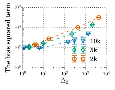
Figure 6: In the fixed design setting, the bias squared term of the generalization performance grows with $\Delta_{2}$.

In our experiments, we compute the value of the bias squared term and $\Delta_{2}$ on the Census dataset. To gain statistically meaningful insights, we collect and average the value of $\frac{\lambda^{2}}{n}\bar{y}^{T}(\tilde{K}+\lambda I)^{-2}\bar{y}$ and $\Delta_{2}$ using 3 independent runs with different random seeds. In Figure 6, we plot the value of $\frac{\lambda^{2}}{n}\bar{y}^{T}(\tilde{K}+\lambda I)^{-2}\bar{y}$ as a function of $\Delta_{2}$ for 3 different numbers of features; by controlling the number of features, we can demonstrate the influence of $\Delta_{2}$ while $\Delta_{1}$ is held roughly fixed. In each curve in Figure 6, the data points are collected from FP-RFFs, circulant FP-RFFs, as well as LP-RFFs using $\{1,2,4,8\}$ bit precision. We can see that for each number of features, the value of $\frac{\lambda^{2}}{n}\bar{y}^{T}(\tilde{K}+\lambda I)^{-2}\bar{y}$ grows with $\Delta_{2}$. These results demonstrate that the upper bound on the bias term in Proposition 1 is quite loose, and is not capturing the influence of $\Delta_{2}$ properly.

Appendix C THEORETICAL GUARANTEES FOR LP-RFFS

In this section, we first lower bound the probability that using LP-RFFs results in a kernel approximation matrix that is a $(\Delta_{1},\Delta_{2})$-spectral approximation of the exact kernel matrix (Section C.1). We then present bounds on the Frobenius kernel approximation error for LP-RFFs (Section C.2).

C.1 $(\Delta_{1},\Delta_{2})$-Spectral Approximation Bounds for LP-RFFs

As usual, let $K\in\mathbb{R}^{n\times n}$ denote the kernel matrix, and $Z\in\mathbb{R}^{n\times m}$ be the random Fourier feature matrix, where $n$ is the number of data points and $m$ is the number of features. We can write $Z=\frac{1}{\sqrt{m}}\begin{bmatrix}z_{1},\dots,z_{m}\end{bmatrix}$ where $z_{i}$ are the (scaled) columns of $Z$. Each entry of $Z$ has the form $\sqrt{2/m}\cos(w^{T}x+a)$ for some $w,x\in\mathbb{R}^{d}$ and $a\in\mathbb{R}^{m}$, where $d$ is the dimension of the original dataset. Then $\mathbb{E}[z_{i}z_{i}^{T}]=K$, so $\mathbb{E}[ZZ^{T}]=K$.

Now suppose we quantize $Z$ to $b$ bits using the quantization method described in Section 4.1, for some fixed $b\geq 1$. Then the quantized feature matrix is $Z+C$ for some random $C\in\mathbb{R}^{n\times m}$ whose entries are independent conditioned on $Z$ (but not identically distributed) with $\mathbb{E}[C\mid Z]=0$. We can write $C=\frac{1}{\sqrt{m}}\begin{bmatrix}c_{1},\dots,c_{m}\end{bmatrix}$ where $c_{i}$ are the (scaled) columns of $C$. Moreover, the $c_{i}$ are independent conditioned on $Z$. Defining $\delta^{2}_{b}:=\frac{2}{(2^{b}-1)^{2}}$, the entries $C_{ij}$ have variance $\mathbb{E}[C_{ij}^{2}\mid Z_{ij}]\leq\delta_{b}^{2}/m$ by Proposition 7 in Appendix C.2. In terms of the vectors $c_{i}$, we can also see that $\mathbb{E}[c_{i,j}^{2}\mid Z_{ij}]\leq\delta_{b}^{2}$, where $c_{i,j}$ denotes the $j^{th}$ element of $c_{i}$.

We first analyze the expectation of $(Z+C)(Z+C)^{T}$ (over both the randomness of $Z$ and of $C$).

Lemma 3.

$\mathbb{E}[(Z+C)(Z+C)^{T}]=K+D$, where $D:=\mathbb{E}[c_{1}c_{1}^{T}]=s_{b}I_{n}$ is a multiple of the identity, for $0\leq s_{b}\leq\delta_{b}^{2}$. $D$ does not depend on the number of random features $m$.

Proof.

$$\mathbb{E}[(Z+C)(Z+C)^{T}]=\mathbb{E}\bigg{[}\frac{1}{m}\sum_{i=1}^{m}(z_{i}+c_{i})(z_{i}+c_{i})^{T}\bigg{]}=\mathbb{E}[(z_{1}+c_{1})(z_{1}+c_{1})^{T}]$$

Since $\mathbb{E}_{c_{1}}[c_{1}\mid z_{1}]=0$, it follows that

$$\mathbb{E}[(z_{1}+c_{1})(z_{1}+c_{1})^{T}] = \mathbb{E}_{z_{1}}\Big{[}\mathbb{E}_{c_{1}}[(z_{1}+c_{1})(z_{1}+c_{1})^{T}\mid z_{1}]\Big{]}$$

$$= \mathbb{E}_{z_{1}}[z_{1}z_{1}^{T}]+\mathbb{E}_{z_{1}}\Big{[}\mathbb{E}_{c_{1}}[c_{1}c_{1}^{T}\mid z_{1}]\Big{]}$$

$$= K+\mathbb{E}[c_{1}c_{1}^{T}]$$

It is clear that $D:=\mathbb{E}[c_{1}c_{1}^{T}]$ is a diagonal matrix, because each element of $c_{1}$ is a zero-mean independent random variable. It is also easy to see that the $j^{th}$ entry on the diagonal of $D$ is equal to $\mathbb{E}[c_{1,j}^{2}\mid z_{1,j}]\leq\delta_{b}^{2}$. Lastly, we argue that each element $z_{1,j}=\sqrt{2}\cos(w_{1}^{T}x_{j}+a_{1})$ has the same distribution, because it is distributed the same as $\sqrt{2}\cos(a_{1})$ for $a_{1}$ uniform in $[0,2\pi]$. Thus, $\mathbb{E}[c_{1,j}^{2}\mid z_{1,j}]$ is independent of $j$. Letting $s_{b}:=\mathbb{E}[c_{1,1}^{2}\mid z_{1,1}]\leq\delta_{b}^{2}$ completes the proof.

∎

With $D:=\mathbb{E}[c_{1}c_{1}^{T}]$, we can use matrix concentration to show that the quantized kernel matrix $\tilde{K}=(Z+C)(Z+C)^{T}$ is close to its expectation $K+D$. We first strengthen the matrix Bernstein inequality with intrinsic dimension (Theorem 7.7.1 in Tropp (2015)) by removing the requirement on the deviation.

Theorem 4 (Matrix Bernstein: Hermitian Case with Intrinsic Dimension).

Consider a finite sequence $\{X_{k}\}$ of random Hermitian matrices of the same size, and assume that

$$\mathbb{E}[X_{k}]=0\quad\text{and}\quad\lambda_{\max}(X_{k})\leq L\quad\text{for each index $k$.}$$

Introduce the random matrix

$$Y=\sum\nolimits_{k}X_{k}.$$

Let $V$ be a semidefinite upper bound for the matrix-valued variance $\mathbb{VAR}\left[Y\right]$:

$$V\succeq\mathbb{VAR}\left[Y\right]=\mathbb{E}[Y^{2}]=\sum\nolimits_{k}\mathbb{E}[X_{k}^{2}].$$

Define the intrinsic dimension bound and variance bound

$$\operatorname{intdim}(V)=\frac{\mathop{\rm tr}(V)}{\|V\|}\quad\text{and}\quad v=\|V\|.$$

Then, for $t\geq 0$,

$$\mathbb{P}\left(\lambda_{\max}(Y)\geq t\right)\leq 4\operatorname{intdim}(V)\cdot\exp\left(\frac{-t^{2}/2}{v+Lt/3}\right).$$ (4)

Proof.

The case of $t\geq\sqrt{v}+L/3$ is exactly Theorem 7.7.1 in Tropp (2015). We just need to show that the bound is vacuous when $0\leq t<\sqrt{v}+L/3$.

Suppose that $0\leq t<\sqrt{v}+L/3$. We show that then $t^{2}\leq 2(v+Lt/3)$. Indeed, $t^{2}-2Lt/3-2v$ has roots $\frac{L}{3}\pm\sqrt{\frac{L^{2}}{9}+2v}$. The condition $t^{2}\leq 2(v+Lt/3)$ is then equivalent to

$$\frac{L}{3}-\sqrt{\frac{L^{2}}{9}+2v}\leq t\leq\frac{L}{3}+\sqrt{\frac{L^{2}}{9}+2v}.$$

The lower bound is negative since $v\geq 0$, and $t<\sqrt{v}+L/3$ implies $t<L/3+\sqrt{L^{2}/9+2v}$, satisfying the upper bound. Thus $0\leq t<\sqrt{v}+L/3$ implies that $t^{2}\leq 2(v+Lt/3)$. The bound in equation (4) becomes

$$4\operatorname{intdim}(V)\exp\left(-\frac{t^{2}/2}{v+Lt/3}\right)\geq 4\operatorname{intdim}(V)\exp(-1)\geq 4/e>1,$$

since $\operatorname{intdim}(V)\geq 1$. Thus (4) holds vacuously for $0\leq t<\sqrt{v}+L/3$. ∎

We now present Lemma 5, in which we lower bound the probability that $\tilde{K}$ is “close” to its expectation $K+D$, in the specific sense we describe below.

Lemma 5.

Let $K$ be an exact kernel matrix, and $\tilde{K}=(Z+C)(Z+C)^{T}$ be an $m$-features $b$-bit LP-RFF approximation of $K$ with expectation $K+D$. For any deterministic matrix $B$, let $L:=2n\|B\|^{2}$ and $M:=B(K+\delta^{2}_{b}I_{n})B^{T}$, then for any $t_{1},t_{2}\geq 0$,

$$\mathbb{P}\bigg{[}-t_{1}I_{n}\preceq B\Big{(}(Z+C)(Z+C)^{T}-(K+D)\Big{)}B\preceq t_{2}I_{n}\bigg{]}$$

$$\geq\ 1-\frac{4\mathop{\rm tr}(M)}{\|M\|}\left[\exp\left(\frac{-mt_{1}^{2}}{2L(\|M\|+2t_{1}/3)}\right)+\exp\left(\frac{-mt_{2}^{2}}{2L(\|M\|+2t_{2}/3)}\right)\right].$$

Proof.

Let $S_{i}=\frac{1}{m}\left(B(z_{i}+c_{i})(z_{i}+c_{i})^{T}B^{T}-B(K+D)B^{T}\right)$ and $S=\sum_{i=1}^{m}S_{i}=B\left((Z+C)(Z+C)^{T}-(K+D)\right)B$. We see that $\mathbb{E}[S_{i}]=0$. We will bound $\lambda_{\max}(S)$ and $\lambda_{\min}(S)$ by applying the matrix Bernstein inequality for symmetric matrices with intrinsic dimension (Theorem 4). Thus we need to bound $\|S_{i}\|$ and $\|\sum_{i=1}^{m}\mathbb{E}[S_{i}^{2}]\|$.

Let $u_{i}=B(z_{i}+c_{i})\in\mathbb{R}^{n}$, then $S_{i}=\frac{1}{m}(u_{i}u_{i}^{T}-\mathbb{E}[u_{i}u_{i}^{T}])$. We first bound $\|u_{i}u_{i}^{T}\|$. Since this is a rank 1 matrix,

$$\|u_{i}u_{i}^{T}\|=\|u_{i}\|^{2}=\|B(z_{i}+c_{i})\|^{2}\leq\|B\|^{2}\|z_{i}+c_{i}\|^{2}\leq 2n\|B\|^{2},$$

where we have used the fact that $z_{i}+c_{i}$ is a vector of length $n$ whose entries are in $[-\sqrt{2},\sqrt{2}]$. This gives a bound on $\|S_{i}\|$:

$$\|S_{i}\|=\frac{1}{m}\|u_{i}u_{i}^{T}-\mathbb{E}[u_{i}u_{i}^{T}]\|\leq\frac{1}{m}\|u_{i}u_{i}^{T}\|+\frac{1}{m}\mathbb{E}\|u_{i}u_{i}^{T}\|\leq\frac{4n\|B\|^{2}}{m}=2L/m.$$

Thus $\lambda_{\max}(S_{i})\leq 2L/m$ and $\lambda_{\max}(-S_{i})=-\lambda_{\min}(S_{i})\leq 2L/m$.

Now it’s time to bound $\mathbb{E}[S_{i}^{2}]$. We will use

$$\mathbb{E}[S_{i}^{2}] = \frac{1}{m^{2}}\Big{(}\mathbb{E}\big{[}(u_{i}u_{i}^{T})^{2}\big{]}-\mathbb{E}\big{[}u_{i}u_{i}^{T}\big{]}^{2}\Big{)}\preceq\frac{1}{m^{2}}\mathbb{E}[(u_{i}u_{i}^{T})^{2}]=\frac{1}{m^{2}}\mathbb{E}[u_{i}u_{i}^{T}u_{i}u_{i}^{T}]$$

$$= \frac{1}{m^{2}}\mathbb{E}[\|u_{i}\|^{2}u_{i}u_{i}^{T}]\preceq\frac{2n\|B\|^{2}}{m^{2}}\mathbb{E}[u_{i}u_{i}^{T}].$$

Thus

$$\sum_{i=1}^{m}\mathbb{E}[S_{i}^{2}]\preceq\frac{2n\|B\|^{2}}{m}\mathbb{E}[v_{1}v_{1}^{T}]=\frac{2n\|B\|^{2}}{m}B(K+D)B^{T}\preceq\frac{2n\|B\|^{2}}{m}B(K+\delta^{2}_{b}I_{n})B^{T}=LM/m.$$

Applying Theorem 4 with $S$, for any $t_{2}\geq 0$, we have

$$\mathbb{P}\bigg{[}\lambda_{\max}(B\Big{(}(Z+C)(Z+C)^{T}-(K+D)\Big{)}B)\succeq t_{2}I_{n}\bigg{]}\leq\frac{4\mathop{\rm tr}(M)}{\|M\|}\exp\left(\frac{-mt_{2}^{2}}{2L(\|M\|+2t_{2}/3)}\right).$$

Similarly, applying Theorem 4 with $-S$ and using the fact that $\lambda_{\max}(-S)=-\lambda_{\min}(S)$, for any $t_{1}\geq 0$, we have

$$\mathbb{P}\bigg{[}\lambda_{\min}(B\Big{(}(Z+C)(Z+C)^{T}-(K+D)\Big{)}B)\preceq-t_{1}I_{n}\bigg{]}\leq\frac{4\mathop{\rm tr}(M)}{\|M\|}\exp\left(\frac{-mt_{1}^{2}}{2L(\|M\|+2t_{1}/3)}\right).$$

Combining the two bounds with the union bound yields the desired inequality. ∎

We are now ready to show that low-precision features yield close spectral approximation to the exact kernel matrix.

Theorem 2.

Let $\tilde{K}$ be an $m$-feature $b$-bit LP-RFF approximation of a kernel matrix $K$, and assume $\|K\|\geq\lambda\geq\delta^{2}_{b}:=2/(2^{b}-1)^{2}$. Then for any $\Delta_{1}\geq 0$, $\Delta_{2}\geq\delta^{2}_{b}/\lambda$,

$$\mathbb{P}\Big{[}(1-\Delta_{1}) (K+\lambda I)\preceq\tilde{K}+\lambda I\preceq(1+\Delta_{2})(K+\lambda I)\Big{]}\geq$$

$$1-8\mathop{\rm tr}\left((K+\lambda I_{n})^{-1}(K+\delta^{2}_{b}I_{n})\right)\left(\exp\left(\frac{-m\Delta_{1}^{2}}{\frac{4n}{\lambda}(1+\frac{2}{3}\Delta_{1})}\right)+\exp\left(\frac{-m(\Delta_{2}-\frac{\delta^{2}_{b}}{\lambda})^{2}}{\frac{4n}{\lambda}(1+\frac{2}{3}(\Delta_{2}-\frac{\delta^{2}_{b}}{\lambda}))}\right)\right).$$

Proof.

We conjugate the desired inequality with $B:=(K+\lambda I_{n})^{-1/2}$ (i.e., multiply by $B$ on the left and right), noting that semidefinite ordering is preserved by conjugation:

$$(1-\Delta_{1})(K+\lambda I_{n})\preceq\tilde{K}+\lambda I_{n}\preceq(1+\Delta_{2})(K+\lambda I_{n})$$

$$\iff\ (1-\Delta_{1})I_{n}\preceq B(\tilde{K}+\lambda I_{n})B\preceq(1+\Delta_{2})I_{n}$$

$$\iff\ -\Delta_{1}I_{n}\preceq B(\tilde{K}+\lambda I_{n})B-I_{n}\preceq\Delta_{2}I_{n}$$

$$\iff\ -\Delta_{1}I_{n}\preceq B(\tilde{K}+\lambda I_{n}-K-\lambda I_{n})B\preceq\Delta_{2}I_{n}$$

$$\iff\ -\Delta_{1}I_{n}\preceq B(\tilde{K}-K)B\preceq\Delta_{2}I_{n}.$$

We show that $-\Delta_{1}I_{n}\preceq B(\tilde{K}-K-D)B\preceq(\Delta_{2}-\delta^{2}_{b}/\lambda)I_{n}$ implies $-\Delta_{1}I_{n}\preceq B(\tilde{K}-K)B\preceq\Delta_{2}I_{n}$. Indeed, $\|BDB\|\leq\delta^{2}_{b}/\lambda$ because $\|B\|^{2}=\|B^{2}\|=\|(K+\lambda I_{n})^{-1}\|\leq 1/\lambda$ and $\|D\|\leq\delta_{b}^{2}$, so $BDB\preceq(\delta^{2}_{b}/\lambda)I_{n}$. Moreover, since $D\succeq 0$ by Lemma 3 and $B$ is symmetric, $BDB\succeq 0$. Thus the condition $-\Delta_{1}I_{n}\preceq B(\tilde{K}-K-D)B\preceq(\Delta_{2}-\delta^{2}_{b}/\lambda)I_{n}$ implies:

$$B(\tilde{K}-K)B =B(\tilde{K}-K-D)B+BDB\preceq(\Delta_{2}-\delta^{2}_{b}/\lambda)I_{n}+\delta^{2}_{b}/\lambda I_{n}=\Delta_{2}I_{n},$$

$$B(\tilde{K}-K)B =B(\tilde{K}-K-D)B+BDB\succeq-\Delta_{1}I_{n}+0=-\Delta_{1}I_{n}.$$

Hence $\mathbb{P}\left[-\Delta_{1}I_{n}\preceq B(\tilde{K}-K)B\preceq\Delta_{2}I_{n}\right]\geq\mathbb{P}\left[-\Delta_{1}I_{n}\preceq B(\tilde{K}-K-D)B\preceq(\Delta_{2}-\delta^{2}_{b}/\lambda)I_{n}\right]$. It remains to show that $-\Delta_{1}I_{n}\preceq B(\tilde{K}-K-D)B\preceq(\Delta_{2}-\delta^{2}_{b}/\lambda)I_{n}$ with the desired probability, by applying Lemma 5. We apply Lemma 5 for $B:=(K+\lambda I_{n})^{-1/2}$, $L:=2n\|B\|^{2}\leq 2n/\lambda$, and $M:=B(K+\delta^{2}_{b}I_{n})B$.

To simplify the bound one gets from applying Lemma 5 with the above $B$, $L$, and $M$, we will use the following expression for $\mathop{\rm tr}(M)$, and the following upper and lower bounds on $\|M\|$. $\mathop{\rm tr}(M)=\mathop{\rm tr}\Big{(}B^{2}(K+\delta^{2}_{b}I_{n})\Big{)}=\mathop{\rm tr}\Big{(}(K+\lambda I_{n})^{-1}(K+\delta^{2}_{b}I_{n})\Big{)}$. Letting $K=USU^{T}$ be the SVD of $K$, we get that $M=U(S+\lambda I_{n})^{-1/2}U^{T}U(S+\delta^{2}_{b}I_{n})U^{T}U(S+\lambda I_{n})^{-1/2}U^{T}=U(S+\lambda I_{n})^{-1}(S+\delta^{2}_{b}I_{n})U^{T}$. Thus, letting $\lambda_{1}$ be the largest eigenvalue of $K$ (recall $\lambda_{1}\geq\lambda$ by assumption), $\|M\|=(\lambda_{1}+\delta^{2}_{b})/(\lambda_{1}+\lambda)\geq(\lambda_{1}+\delta^{2}_{b})/(2\lambda_{1})\geq 1/2$. We also assume that $\delta^{2}_{b}\leq\lambda$, so $\|M\|\leq 1$. Lemma 5 allows us to conclude the following:

$$\mathbb{P}\bigg{[}(1-\Delta_{1})(K+\lambda I_{n})\preceq\tilde{K}+\lambda I_{n}\preceq(1+\Delta_{2})(K+\lambda I_{n})\bigg{]}$$

$$= \;\;\mathbb{P}\bigg{[}-\Delta_{1}I_{n}\preceq B(\tilde{K}-K)B\preceq\Delta_{2}I_{n}\bigg{]}$$

$$\geq \;\;\mathbb{P}\left[-\Delta_{1}I_{n}\preceq B(\tilde{K}-(K+D))B\preceq(\Delta_{2}-\delta^{2}_{b}/\lambda)I_{n}\right]$$

$$\geq \;\;1-\frac{4\mathop{\rm tr}(M)}{\|M\|}\left[\exp\left(\frac{-m\Delta_{1}^{2}}{2L(\|M\|+2\Delta_{1}/3)}\right)+\exp\left(\frac{-m(\Delta_{2}-\delta^{2}_{b}/\lambda)^{2}}{2L(\|M\|+2(\Delta_{2}-\delta^{2}_{b}/\lambda)/3)}\right)\right]$$

$$\geq \;\;1-8\mathop{\rm tr}\left((K+\lambda I_{n})^{-1}(K+\delta^{2}_{b}I_{n})\right)\left[\exp\left(\frac{-m\Delta_{1}^{2}}{4n/\lambda(1+2\Delta_{1}/3)}\right)+\exp\left(\frac{-m(\Delta_{2}-\delta^{2}_{b}/\lambda)^{2}}{4n/\lambda(1+2(\Delta_{2}-\delta^{2}_{b}/\lambda)/3)}\right)\right].$$

∎

There is a bias-variance trade-off: as we decrease the number of bits $b$, under a fixed memory budget we can use more features, and $(Z+C)(Z+C)^{T}$ concentrates more strongly (lower variance) around the expectation $K+D$ with $0\preceq D\preceq\delta^{2}_{b}I_{n}$. However, this expectation is further away from the true kernel matrix $K$ (larger bias). Thus there should be an optimal number of bits $b^{*}$ that balances the bias and the variance.

Proof of Corollary 2.1.

Letting $\Delta_{2}\to\infty$ in Theorem 2 gives

$$\mathbb{P}\left[(1-\Delta_{1})(K+\lambda I_{n})\preceq\tilde{K}+\lambda I_{n}\right]\geq 1-8\mathop{\rm tr}\left((K+\lambda I_{n})^{-1}(K+\delta^{2}_{b}I_{n})\right)\exp\left(\frac{-m\Delta_{1}^{2}}{4n/\lambda(1+2\Delta_{1}/3)}\right).$$

Using the assumption that $\Delta_{1}\leq 3/2$, we can simplify the bound:

$$\mathbb{P}\left[(1-\Delta_{1})(K+\lambda I_{n})\preceq\tilde{K}+\lambda I_{n}\right]\geq 1-8\mathop{\rm tr}\left((K+\lambda I_{n})^{-1}(K+\delta^{2}_{b}I_{n})\right)\exp\left(\frac{-m\Delta_{1}^{2}}{8n/\lambda}\right).$$

Letting the RHS be $1-\rho$ and solving for $m$ yields

$$m\geq\frac{8n/\lambda}{\Delta_{1}^{2}}\log\Big{(}\frac{a}{\rho}\Big{)}.$$

Similarly, letting $\Delta_{1}\to\infty$ in Theorem 2 gives

$$\mathbb{P}\left[\tilde{K}+\lambda I_{n}\preceq(1-\Delta_{2})(K+\lambda I_{n})\right]\geq 1-8\mathop{\rm tr}\left((K+\lambda I_{n})^{-1}(K+\delta^{2}_{b}I_{n})\right)\exp\left(\frac{-m(\Delta_{2}-\delta_{b}^{2}/\lambda)^{2}}{4n/\lambda(1+2(\Delta_{2}-\delta_{b}^{2}/\lambda)/3)}\right).$$

Using the assumption that $\Delta_{1}\leq 3/2$, we can simplify the bound:

$$\mathbb{P}\left[(1-\Delta_{1})(K+\lambda I_{n})\preceq\tilde{K}+\lambda I_{n}\right]\geq 1-8\mathop{\rm tr}\left((K+\lambda I_{n})^{-1}(K+\delta^{2}_{b}I_{n})\right)\exp\left(\frac{-m(\Delta_{2}-\delta_{b}^{2}/\lambda)^{2}}{8n/\lambda}\right).$$

Letting the RHS be $1-\rho$ and solving for $m$ yields

$$m\geq\frac{8n/\lambda}{(\Delta_{2}-\delta_{b}^{2}/\lambda)^{2}}\log\Big{(}\frac{a}{\rho}\Big{)}.$$

∎

If we let the number of bits $b$ go to $\infty$ and set $\Delta_{1}=\Delta_{2}=\Delta$, we get the following corollary, similar to the result from Avron et al. (2017):

Corollary 5.1.

Suppose that $\tilde{K}=ZZ^{T}$, $\|K\|\geq\lambda$. Then for any $\Delta\leq 1/2$,

$$\mathbb{P}\left[(1-\Delta)(K+\lambda I_{n})\preceq\tilde{K}+\lambda I_{n}\preceq(1+\Delta)(K+\lambda I_{n})\right]\geq 1-16\mathop{\rm tr}((K+\lambda I_{n})^{-1}K)\exp\left(-\frac{3m\Delta^{2}}{16n/\lambda}\right).$$

Thus if we use $m\geq\frac{16}{3\Delta^{2}}n/\lambda\log(16\mathop{\rm tr}((K+\lambda I_{n})^{-1}K)/\rho)$ features, then $(1-\Delta)(K+\lambda I_{n})\preceq\tilde{K}+\lambda I_{n}\preceq(1+\Delta)(K+\lambda I_{n})$ with probability at least $1-\rho$.

The constants are slightly different from that of Avron et al. (2017) as we use the real features $\sqrt{2}\cos(w^{T}x+a)$ instead of the complex features $\exp(iw^{T}x)$.

From these results, we now know that the number of features required depends linearly on $n/\lambda$; more precisely, we know that if we use $m\geq c_{0}\cdot n/\lambda$ features (for some constant $c_{0}>0$), $\tilde{K}+\lambda I_{n}$ will be a $(\Delta,\Delta)$-spectral approximation of $K+\lambda I_{n}$ with high probability. Avron et al. (2017) further provide a lower bound, showing that if $m\leq c_{1}\cdot n/\lambda$ (for some other constant $c_{1}>0$), $\tilde{K}+\lambda I_{n}$ will not be a $(\Delta,\Delta)$-spectral approximation of $K+\lambda I_{n}$ with high probability. This shows that the number of random Fourier features must depend linearly on $n/\lambda$.

C.2 Frobenius Kernel Approximation Error Bounds for LP-RFFs

We begin this section by bounding the variance of the quantization noise $C$ added to the random feature matrix $Z$. We prove this as a simple consequence of the following Lemma.

Lemma 6.

For $z\in[a,c]$, let $X_{z}^{a,c}$ be the random variable which with probability $\frac{z-a}{c-a}$ equals $c-z$, and with probability $\frac{c-z}{c-a}$ equals $a-z$. Then $\mathbb{E}\left[X_{z}^{a,c}\right]=0$, and $\mathbb{VAR}\left[X_{z}^{a,c}\right]=(c-z)(z-a)\leq\frac{(c-a)^{2}}{4}$.

Proof.

$$\mathbb{E}\left[X_{z}^{a,c}\right] = (c-z)\cdot\frac{z-a}{c-a}+(a-z)\cdot\frac{c-z}{c-a}$$

$$= 0.$$

$$\mathbb{VAR}\left[X_{z}^{a,c}\right] = (c-z)^{2}\cdot\frac{z-a}{c-a}+(a-z)^{2}\cdot\frac{c-z}{c-a}$$

$$= \frac{(c-z)(z-a)((c-z+z-a))}{c-a}$$

$$= (c-z)(z-a)$$

$$\frac{d}{dz}[\mathbb{VAR}\left[X_{z}^{a,c}\right]] = \frac{d}{dz}[-z^{2}+(c+a)z-ac]$$

$$= -2z+c+a.$$

Now, setting the derivative to 0 gives $z^{*}=\frac{c+a}{2}$. Thus, $\operatorname*{arg\,max}_{z\in[a,c]}(c-z)(z-a)=\frac{c+a}{2}$, and $\max_{z\in[a,c]}(c-z)(z-a)=(c-\frac{c+a}{2})(\frac{c+a}{2}-a)=\frac{(c-a)^{2}}{4}$. ∎

Proposition 7.

$\mathbb{E}[C_{ij}^{2}\mid Z_{ij}]\leq\delta_{b}^{2}/m$, for $\delta_{b}^{2}:=\frac{2}{(2^{b}-1)^{2}}$.

Proof.

Given a feature $Z_{ij}\in[-\sqrt{2/m},\sqrt{2/m}]$, we quantize it to $b$ bits by dividing this interval into $2^{b}-1$ equally-sized sub-intervals (each of size $\frac{2\sqrt{2/m}}{2^{b}-1}$), and randomly rounding to the top or bottom of the sub-interval containing $Z_{ij}$ (in an unbiased manner). Let $a,c$ denote the boundaries of the sub-interval containing $Z_{ij}$, where $c=a+\frac{2\sqrt{2/m}}{2^{b}-1}$. We can now see that $C_{ij}=X_{Z_{ij}}^{a,c}$ is the unique random variable such that $Z_{ij}+C_{ij}\in\{a,c\}$ and $\mathbb{E}\left[C_{ij}\mid Z_{ij}\right]=0$. Because $c-a=\frac{2\sqrt{2/m}}{2^{b}-1}$, it follows from Lemma 6 that $\mathbb{E}[C_{ij}^{2}\mid Z_{ij}]=\mathbb{VAR}\left[X_{Z_{ij}}^{a,c}\mid Z_{ij}\right]\leq\frac{(c-a)^{2}}{4}=\frac{8/m}{4(2^{b}-1)^{2}}=\delta_{b}^{2}/m$. ∎

We now prove an upper bound on the expected kernel approximation error for LP-RFFs, which applies for any quantization function with bounded variance. This error corresponds exactly to the variance of the random variable which is the product of two quantized random features.

Theorem 8.

For $x,y\in\mathcal{X}$, assume we have random variables $Z_{x},Z_{y}$ satisfying $\mathbb{E}\left[Z_{x}Z_{y}\right]=k(x,y)$, $\mathbb{VAR}\left[Z_{x}Z_{y}\right]\leq\sigma^{2}$, and that $k(x,x)=k(y,y)=1$. For any unbiased random quantization function $Q$ with bounded variance $\mathbb{VAR}\left[Q(z)\right]\leq\tilde{\sigma}^{2}$ for any (fixed) $z$, it follows that $\mathbb{E}\left[Q(Z_{x})Q(Z_{y})\right]=k(x,y)$, and that $\mathbb{VAR}\left[Q(Z_{x})Q(Z_{y})\right]\leq 2\tilde{\sigma}^{2}+\tilde{\sigma}^{4}+\sigma^{2}$.

Proof.

Let $Q(Z_{x})=Z_{x}+\epsilon_{x}$, and $Q(Z_{y})=Z_{y}+\epsilon_{y}$, where $\mathbb{E}\left[\epsilon_{x}\right]=\mathbb{E}\left[\epsilon_{y}\right]=0$, $\mathbb{E}\left[\epsilon_{x}^{2}\right]\leq\tilde{\sigma}^{2}$, $\mathbb{E}\left[\epsilon_{y}^{2}\right]\leq\tilde{\sigma}^{2}$, and $\epsilon_{x}$,$\epsilon_{y}$ are independent random variables.

$$\mathbb{E}\left[Q(Z_{x})Q(Z_{y})\right] = \mathbb{E}\left[(Z_{x}+\epsilon_{x})(Z_{y}+\epsilon_{y})\right]$$

$$= \mathbb{E}\left[Z_{x}Z_{y}+Z_{y}\epsilon_{x}+Z_{x}\epsilon_{y}+\epsilon_{x}\epsilon_{y}\right]$$

$$= \mathbb{E}\left[Z_{x}Z_{y}\right]$$

$$= k(x,y).$$

$$\mathbb{VAR}\left[Q(Z_{x})Q(Z_{y})\right] = \mathbb{E}\left[\Big{(}Q(Z_{x})Q(Z_{y})-k(x,y)\Big{)}^{2}\right]$$

$$= \mathbb{E}\left[\Big{(}(Z_{x}+\epsilon_{x})(Z_{y}+\epsilon_{y})-k(x,y)\Big{)}^{2}\right]$$

$$= \mathbb{E}\left[\Big{(}Z_{y}\epsilon_{x}+Z_{x}\epsilon_{y}+\epsilon_{x}\epsilon_{y}+Z_{x}Z_{y}-k(x,y)\Big{)}^{2}\right]$$

$$= \mathbb{E}\left[\Big{(}Z_{y}\epsilon_{x}+Z_{x}\epsilon_{y}+\epsilon_{x}\epsilon_{y}\Big{)}^{2}\right]+\mathbb{E}\left[\Big{(}Z_{x}Z_{y}-k(x,y)\Big{)}^{2}\right]$$

$$\leq \mathbb{E}\left[Z_{y}^{2}\epsilon_{x}^{2}+Z_{x}^{2}\epsilon_{y}^{2}+\epsilon_{x}^{2}\epsilon_{y}^{2}\right]+\sigma^{2}$$

$$\leq k(y,y)\tilde{\sigma}^{2}+k(x,x)\tilde{\sigma}^{2}+\tilde{\sigma}^{4}+\sigma^{2}$$

$$= 2\tilde{\sigma}^{2}+\tilde{\sigma}^{4}+\sigma^{2}.$$

Note that if $x=y$, for this proof to hold, we would need to randomly quantize $Z_{x}$ twice, giving two independent quantization noise samples $\epsilon_{x}^{(1)}$ and $\epsilon_{x}^{(2)}$. ∎

This theorem suggests that if $2\tilde{\sigma}^{2}+\tilde{\sigma}^{4}\ll\sigma^{2}$, quantizing the random features will have negligable effect on the variance. In practice, for the random quantization method we use with random Fourier features (described in Section 4.1), we have $\tilde{\sigma}^{2}=\frac{2}{(2^{b}-1)^{2}}$. Thus, for a large enough precision $b$, the quantization noise will be tiny relative to the variance inherent to the random features.

We note that the above theorem applies to one-dimensional random features, but can be trivially extended to $m$ dimensional random features. We show this in the following corollary.

Corollary 8.1.

For $x,y\in\mathcal{X}$, assume we have random variables $Z_{x},Z_{y}$ satisfying $\mathbb{E}\left[Z_{x}Z_{y}\right]=k(x,y)$, and $\mathbb{VAR}\left[Z_{x}\right],\mathbb{VAR}\left[Z_{y}\right]\leq\sigma^{2}$, and that $k(x,x)=k(y,y)=1$. Let $Q$ be any unbiased quantization function with bounded variance ($\mathbb{E}\left[Q(z)\right]=z$, $\mathbb{VAR}\left[Q(z)\right]\leq\tilde{\sigma}^{2}$ for any $z$). Let $S=Z_{x}Z_{y}$, $T=Q(Z_{x})Q(Z_{y})$, and $(S_{1},\ldots,S_{n})$, $(T_{1},\ldots,T_{n})$ be a random sequence of i.i.d. draws from $S$ and $T$ respectively. Define $\bar{S}_{n}=\frac{1}{n}\sum_{i=1}^{n}S_{i}$, and $\bar{T}_{n}=\frac{1}{n}\sum_{i=1}^{n}T_{i}$, to be the empirical mean of these draws. It follows that $\mathbb{E}\left[\bar{S}_{n}\right]=\mathbb{E}\left[\bar{T}_{n}\right]=k(x,y)$, and that $\mathbb{VAR}\left[\bar{S}_{n}\right]\leq\frac{\sigma^{2}}{n}$, and $\mathbb{VAR}\left[\bar{T}_{n}\right]\leq\frac{2\tilde{\sigma}^{2}+\tilde{\sigma}^{4}+\sigma^{2}}{n}$.

Proof.

$$\mathbb{VAR}\left[\bar{S}_{n}\right] = \mathbb{VAR}\left[\frac{1}{n}\sum_{i=1}^{n}S_{i}\right]$$

$$= \sum_{i=1}^{n}\mathbb{VAR}\left[\frac{1}{n}S_{i}\right]$$

$$\leq n\cdot\frac{\sigma^{2}}{n^{2}}$$

$$= \frac{\sigma^{2}}{n}$$

The result for $\mathbb{VAR}\left[\bar{T}_{n}\right]$ follows in the same way, using the result from Theorem 8. ∎

Appendix D EXPERIMENT DETAILS AND EXTENDED RESULTS

D.1 Datasets and Details Applying to All Experiments

In this work, we present results using FP-Nyström, FP-RFFs, circulant FP-RFFs, and LP-RFFs on the TIMIT, YearPred, CovType, and Census datasets. These datasets span regression, binary classification, and multi-class classification tasks. We present details about these datasets in Table 3. In these experiments we use the Gaussian kernel with the bandwidth $\sigma$ specified in Table 4; we use the same bandwidths as May et al. (2017). To evaluate the performance of these kernel models, we measure the classification error for classification tasks, and the mean squared error (MSE) for regression tasks ($\frac{1}{n}\sum_{i=1}^{n}(f_{\tilde{K}}(x_{i})-y_{i})^{2}$), on the heldout set. We compute the total memory utilization as the sum of all the components in Table 1.

Table 3: Dataset details. For classification tasks, we write the number of classes in parentheses in the “task” column.

Dataset	Task	Train	Heldout	Test	# Features
Census	Reg.	16k	2k	2k	119
YearPred	Reg.	417k	46k	52k	90
CovType	Class. (2)	418k	46k	116k	54
TIMIT	Class. (147)	2.3M	245k	116k	440

Table 4: The Gaussian kernel bandwidths used, and the search grid for initial learning rate on the Census, YearPred, Covtype and TIMIT datasets. Optimal learning rate in bold.

Dataset	$1/2\sigma^{2}$	Initial learning rate grid
Census	0.0006	0.01, 0.05, 0.1, 0.5, 1.0
YearPred	0.01	0.05, 0.1, 0.5, 1.0, 5.0
Covtype	0.6	1.0, 5.0, 10.0, 50.0, 100.0
TIMIT	0.0015	5.0, 10.0, 50.0, 100.0, 500.0

For all datasets besides TIMIT, we pre-processed the features and labels as follows: We normalized all continuous features to have zero mean and unit variance. We did not normalize the binary features in any way. For regression datasets, we normalized the labels to have zero mean across the training set.

TIMIT (Garofolo et al., 1993) is a benchmark dataset in the speech recognition community which contains recordings of 630 speakers, of various English dialects, each reciting ten sentences, for a total of 5.4 hours of speech. The training set (from which the heldout set is then taken) consists of data from 462 speakers each reciting 8 sentences (SI and SX sentences). We use 40 dimensional feature space maximum likelihood linear regression (fMLLR) features (Gales, 1998), and concatenate the 5 neighboring frames in either direction, for a total of 11 frames and 440 features. This dataset has 147 labels, corresponding to the beginning, middle, and end of 49 phonemes. For reference, we use the exact same features, labels, and divisions of the dataset, as (Huang et al., 2014; Chen et al., 2016; May et al., 2017).

We acquired the CovType (binary) and YearPred datasets from the LIBSVM webpage, and the Census dataset from Ali Rahimi’s webpage. For these datasets, we randomly set aside 10% of the training data as a heldout set for tuning the learning rate and kernel bandwidth.

The specific files we used were as follows:

• CovType: We randomly chose 20% of “covtype.libsvm.binary” as test, and used the rest for training/heldout.

• YearPred: We used “YearPredictionMSD” as training/heldout set, and “YearPredictionMSD.t” as test.

• Census: We used the included matlab dataset file “census.mat” from Ali Rahimi’s webpage. This Matlab file had already split the data into train and test. We used a random 10% of the training data as heldout.

D.2 Nyström vs. RFFs (Section 2.2)

We compare the generalization performance of full-precision RFFs and the Nyström method across four datasets, for various memory budgets. We sweep the following hyperparameters: For Nyström, we use $m\in\{1250,2500,5000,10000,20000\}$. For RFFs, we use $m\in\{1250,2500,5000,10000,20000,50000,100000,$ $200000,400000\}$. We choose these limits differently because 20k Nyström features have roughly the same memory footprint as 400k FP-RFFs. For all experiments, we use a mini-batch size of 250. We use a single initial learning rate per dataset across all experiments, which we tune via grid search using 20k Nyström features. We choose to use Nyström features to tune the initial learning rate in order to avoid biasing the results in favor of RFFs. We use an automatic early-stopping protocol, as in (Morgan and Bourlard, 1990; Sainath et al., 2013b, a), to regularize our models (Zhang et al., 2005; Wei et al., 2017) and avoid expensive hyperparameter tuning. It works as follows: at the end of each epoch, we decay the learning rate in half if the heldout loss is less than $1\%$ better relative to the previous best model, using MSE for regression and cross entropy for classification. Furthermore, if the model performs worse than the previous best, we revert the model. The training terminates after the learning rate has been decayed 10 times.

We plot our results comparing the Nyström method to RFFs in Figure 7. We compare the performance of these methods in terms of their number of features, their training memory footprint, and the squared Frobenius norm and spectral norm of their kernel approximation error.

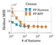
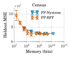
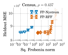
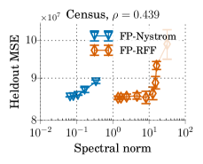
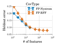
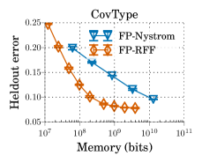
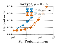
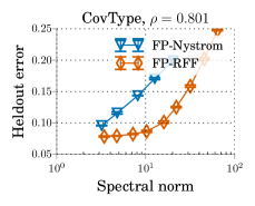
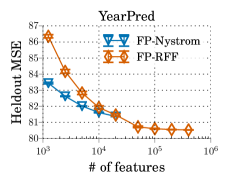
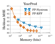
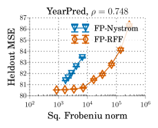
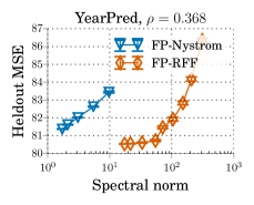
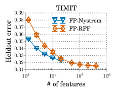
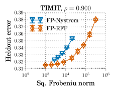
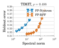
(a)	(b)	(c)	(d)

Figure 7: Generalization performance of FP-RFFs and Nyström with respect to # features (a) and training memory footprint (b) on Census, CovType, Yearpred and TIMIT. Nyström performs better for a fixed number of features, while FP-RFFs perform better under a memory budget. We also see that the relative performance between these methods cannot be fully explained by the Frobenius norms (c) or spectral norms (d) of their respective kernel approximation error matrices; in particular, we see many example of Nyström models that have lower Frobenius or spectral error, but worse heldout performance, than various RFF models. To quantify the degree of alignment between these error metrics and generalization performance (right plots), we show in the figure titles the Spearman rank correlation coefficients $\rho$ between the corresponding $x$ and $y$ metrics. We see in Figure 11 that $1/(1-\Delta_{1})$ attains notably higher values of $\rho$ than the Frobenius and spectral norms of the kernel approximation error. Note that although we plot the average performance across three random seeds for each experimental setting (error bars indicate standard deviation), when we compute the $\rho$ values we treat each experimental result independently (without averaging).

D.3 Nyström vs. RFFs Revisited (Section 3.2)

D.3.1 Small-Scale Experiments

In order to better understand what properties of kernel approximation features lead to strong generalization performance, we perform a more fine-grained analysis on two smaller datasets from the UCI machine learning repository—we consider the Census regression task, and a subset of the CovType task with 20k randomly sampled training points and 20k randomly sampled heldout points. The reason we use these smaller datasets is because computing the spectral norm, as well as ($\Delta_{1}$,$\Delta_{2}$) are expensive operations, which requires instantiating the kernel matrices fully, and performing singular value decompositions. For the Census experiments, we use the closed-form solution for the kernel ridge regression estimator, and choose the $\lambda$ which gives the best performance on the heldout set. For CovType, because there is no closed-form solution for logistic regression, we used the following training protocol to (approximately) find the model which minimizes the regularized training loss (just like the closed-form ridge regression solution does). For each value of $\lambda$, we train the model to (near) convergence using 300 epochs of SGD (mini-batch size 250) at a constant learning rate, and pick the learning rate which gives the lowest regularized training loss for that $\lambda$. We then evaluate this converged model on the heldout set to see which $\lambda$ gives the best performance. We pick the best learning rate, as well as regularization parameter, by using 20k Nyström features as a proxy for the exact kernel (note that because there are only 20k training points, this Nyström approximation is exact). We choose the learning rate $5.0$ from the set $\{0.01,0.05,0.1,0.5,1.0,5.0,10.0,50.0\}$, and the regularization parameter $\lambda=$510-6$$ from $\{$510-8$,$110-7$,$510-7$,$110-6$,$510-6$,$110-5$,$510-5$,$110-4$\}$. For the Census dataset, we pick $\lambda=$510-4$$ from $\{$110-5$,$510-5$,$110-4$,$510-4$,$110-3$,$510-3$,$110-2$,$510-2$,$110-1$\}$. We sweep the number of features shown in Table 5. For both datasets, we report the average squared Frobenius norm, spectral norm, $\Delta$, $(\Delta_{1},\Delta_{2})$ and the average generalization performance, along with standard deviations, using five different random seeds. The results are shown in Figure 8. As can be seen in Figure 8, $1/(1-\Delta_{1})$ aligns much better with generalization performance than the other metrics.

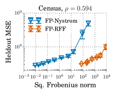
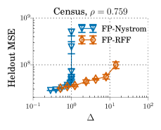
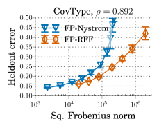
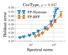
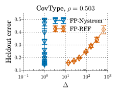
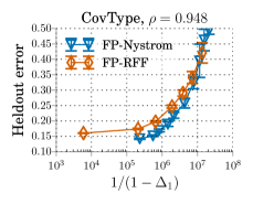
Figure 8: The correlation between generalization performance and squared Frobenius norm, spectral norm, $\Delta$, and $1/(1-\Delta_{1})$ for FP-RFFs and FP-Nyström on the Census and subsampled CovType datasets. To quantify the alignment between these metrics and downstream performance, we include the Spearman rank correlation coefficients $\rho$ computed between these metrics and the downstream performance of our trained models in the figure titles. Note that although we plot the average performance across five random seeds for each experimental setting (error bars indicate standard deviation), when we compute the $\rho$ values we treat each experimental result independently (without averaging).

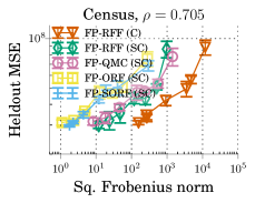
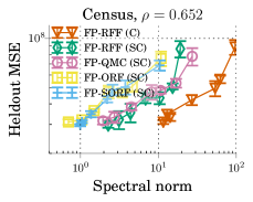
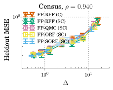
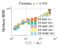
Figure 9: The correlation between generalization performance and squared Frobenius norm, spectral norm, $\Delta$, and $1/(1-\Delta_{1})$ for various types of full-precision RFFs. The Spearman rank correlation coefficients $\rho$ between the $x$ and $y$ metrics of each figure are included in the figure titles. For these full-precision RFF experiments, we see that the original $\Delta$ (Avron et al., 2017) as well as $1/(1-\Delta_{1})$ both align very well with downstream performance ($\rho=0.940$ and $\rho=0.938$, respectively), while the Frobenius and spectral norms do not ($\rho=0.705$ and $\rho=0.652$, respectively). Note that although we plot the average performance across five random seeds for each experimental setting (error bars indicate standard deviation), when we compute the $\rho$ values we treat each experimental result independently (without averaging).

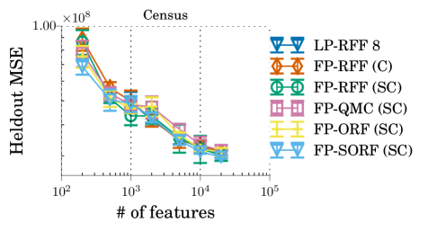
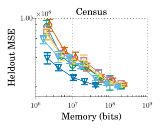
Figure 10: The generalization performance as a function of the number of features (left) and the training memory footprint (right) for various types of RFFs on the Census dataset. We observe that LP-RFFs can achieve lower heldout mean-squared error (MSE) than other types of RFFs, included the memory-efficient structured orthogonal random features (“FP-SORF (SC)”), under the same memory budget. We plot performance averaged over five random seeds, with error bars indicating standard deviations.

Table 5: Number of features used for the different kernel approximation methods in the experiments on generalization performance vs. $(\Delta_{1},\Delta_{2})$ in Sections 3.2 and 5.2.

Methods	Number of features
FP-Nyström	$25,50,100,200,500,1250,2500,5000,10000,20000$
FP-RFF	$200,500,1000,2000,5000,10000,20000$
Cir. FP-RFF	$200,500,1000,2000,5000,10000,20000$
LP-RFF $16$	$500,1000,2000,5000,10000,20000,50000$
LP-RFF $8,4,2,1$	$1000,2000,5000,10000,20000,50000$

It is important to note that although $1/(1-\Delta_{1})$ aligns quite well with generalization performance (Spearman rank correlation coefficients $\rho$ equal to 0.958 and 0.948 on Census and CovType, respectively), it does not align perfectly. In particular, we see that for a fixed value of $\Delta_{1}$, Nyström generally attains better heldout performance than RFFs. We believe this is largely explained by the fact that Nyström always has $\Delta_{2}=0$, while RFFs can have relatively large values of $\Delta_{2}$ when the number of features is small (see Figure 3). As we show in the generalization bound in Proposition 1, in Figure 5, as well as in the empirical and theoretical analysis in Appendix B, we expect generalization performance to deteriorate as $\Delta_{2}$ increases.

D.3.2 Experiments with Different Types of RFFs

In Figure 9 we repeat the above experiment on the Census dataset using a number of variations of RFFs. Specifically, we run experiments using the $[\sin(w^{T}x),\cos(w^{T}x)]$ parameterization of RFFs, which Sutherland and Schneider (2015) show has lower variance than the $\cos(w^{T}x+a)$ parameterization (we denote the $[\sin,\cos]$ method by “FP-RFF (SC)”, and the $\cos$ method by “FP-RFF (C)”). We additionally use Quasi-Monte Carlo features (Yang et al., 2014), as well as orthogonal random features and its structural variant (Yu et al., 2016); we denote these by “FP-QMC (SC)”, “FP-ORF (SC)”, “FP-SORF (SC)” respectively, because we implement them using the $[\sin,\cos]$ parameterization. We can see in Figure 9 that although these methods attain meaningful improvements in the Frobenius and spectral norms of the approximation error, these improvements do not translate into corresponding gains in heldout performance. Once again we see that $1/(1-\Delta_{1})$ is able to much better explain the relative performance between different kernel approximation methods than Frobenius and spectral error. In Figure 10 we see that LP-RFFs outperform these other methods in terms of performance under a memory budget.

D.3.3 Large-Scale $(\Delta_{1},\Delta_{2})$ Experiments

In Figure 11 we plot the performance vs. $1/(1-\Delta_{1})$ on the large-scale experiments from Section 2.2. We measure $\Delta_{1}$ using the exact and approximate kernel matrices on a random subset of 20k heldout points (except for Census, where we use the entire heldout set which has approximately 2k points). We pick several $\lambda$ values between the smallest and largest eigenvalues of the exact (subsampled) training kernel matrix. The strong alignment between generalization performance and $1/(1-\Delta_{1})$ is quite robust to the choice of $\lambda$.

D.3.4 Measuring $\Delta$ and $(\Delta_{1},\Delta_{2})$

In order to measure the $\Delta_{1}$ and $\Delta_{2}$ between a kernel matrix $K$ and an approximation $\tilde{K}$, we first observe that the following statements are equivalent. Note that to get the second statement, we multiply the expressions in the first statement by $(K+\lambda I_{n})^{-1/2}$ on the left and right.

$$(1-\Delta_{1})(K+\lambda I_{n}) \preceq \tilde{K}+\lambda I_{n}\preceq(1+\Delta_{2})(K+\lambda I_{n})$$

$$(1-\Delta_{1})I_{n} \preceq (K+\lambda I_{n})^{-1/2}(\tilde{K}+\lambda I_{n})(K+\lambda I_{n})^{-1/2}\preceq(1+\Delta_{2})I_{n}$$

$$-\Delta_{1}I_{n} \preceq (K+\lambda I_{n})^{-1/2}\Big{(}\tilde{K}+\lambda I_{n}-(K+\lambda I_{n})\Big{)}(K+\lambda I_{n})^{-1/2}\preceq\Delta_{2}I_{n}$$

$$-\Delta_{1}I_{n} \preceq (K+\lambda I_{n})^{-1/2}(\tilde{K}-K)(K+\lambda I_{n})^{-1/2}\preceq\Delta_{2}I_{n}.$$

For $A=(K+\lambda I_{n})^{-1/2}(\tilde{K}-K)(K+\lambda I_{n})^{-1/2}$, this is equivalent to $-\Delta_{1}\leq\lambda_{min}\big{(}A\big{)}$ and $\lambda_{max}\big{(}A\big{)}\leq\Delta_{2}$. Thus, we choose $\Delta_{1}:=-\lambda_{min}\big{(}A\big{)}$ and $\Delta_{2}:=\lambda_{max}\big{(}A\big{)}$. Lastly, we note that $\Delta=\max(\Delta_{1},\Delta_{2})$.

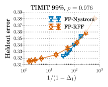
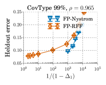
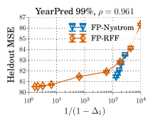
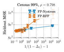
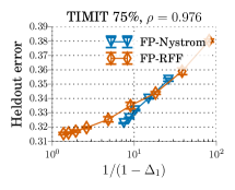
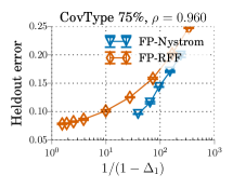
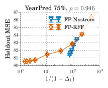
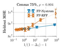
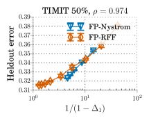
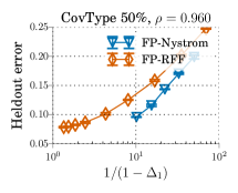
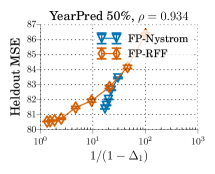
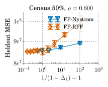
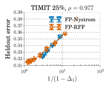
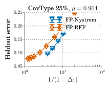
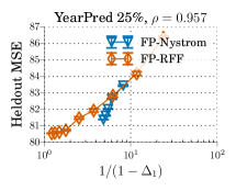
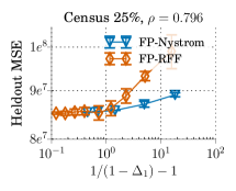
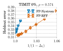
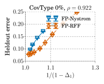
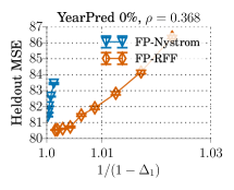
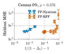
Figure 11: Generalization performance vs. $\frac{1}{1-\Delta_{1}}$, where we measure $\Delta_{1}$ using regularizer strength $\lambda$ equal to the 0, 25, 50, 75, or 99 percentile eigenvalues of the exact kernel matrix (0 percentile indicates largest eigenvalue). Note for the Census dataset, we plot the heldout MSE as a function of $1/(1-\Delta_{1})-1$ to avoid cluttering the data points on the left end of the figure. For comparison to spectral and Frobenius norm plots, see Figure 7. To quantify the degree of alignment between $1/(1-\Delta_{1})$ and generalization performance for these different values of $\lambda$, we compute the Spearman rank correlation coefficients $\rho$. We see $1/(1-\Delta_{1})$ generally attains much higher values of $\rho$ than the Frobenius and spectral approximation errors (Figure 7). Although we plot performance averaged across three random seeds (error bars indicate standard deviations), when we compute $\rho$ we treat each experimental result independently.

D.4 Theory Validation (Section 4.2)

To validate our theory in Section 4.2, we perform two sets of experiments to (1) demonstrate the asymptotic behavior of $\Delta_{1}$ and $\Delta_{2}$ as the number of features increases, and (2) demonstrate that quantization has negligible effect on $\Delta_{2}$ when $\delta_{b}^{2}/\lambda\ll\Delta_{2}$.

To demonstrate the behavior of $\Delta_{1}$ and $\Delta_{2}$ as a function of the number of features, we collect $\Delta_{1}$, and $\Delta_{2}$ using Nyström features, circulant FP-RFFs, and LP-RFFs using $b\in\{1,4,8\}$, on both the Census and the sub-sampled CovType datasets (20k random heldout points). For each approximation, we sweep the number of features as listed in Table 6. We use the same value of $\lambda$ as we used in Section 3.2 for each dataset. In Figure 12, we plot the values of $\Delta_{1}$ and $\Delta_{2}$ attained by these methods as a function of the number of features. As discussed in Section 4.2, $\Delta_{1}$ is primarily determined by the rank of the approximation, and approaches 0 for all the methods as the number of features grows. $\Delta_{2}$, on the other hand, only approaches 0 for the high-precision methods—for $b\in\{1,4\}$, $\Delta_{2}$ converges to higher values (at most $\delta_{b}^{2}/\lambda$, marked by dashed lines).

To demonstrate that quantization has negligible effect on $\Delta_{2}$ when $\delta_{b}^{2}/\lambda\ll\Delta_{2}$, we use 8000 random training points from the Census dataset. For $\lambda\in\{10^{-4},10^{0},10^{4}\}$, and $b\in\{1,2,4,8,16,32\}$, we measure the $\Delta_{2}$ attained by the LP-RFFs relative to the exact kernel matrix. We see that for larger $\lambda$ (corresponding to smaller $\delta_{b}^{2}/\lambda$) in Figure 3, lower precisions can be used while not influencing $\Delta_{2}$ significantly; this aligns with the theory.

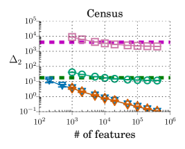
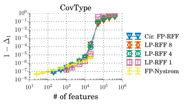
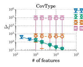
Figure 12: Empirical validation of Theorem 2. As the number of features grows, LP-RFFs approach $\Delta_{1}$ values of 0 (left), but plateau at larger $\Delta_{2}$ for very low precisions (right). These are an extended version of the results from Figure 3 (left, middle) in Section 4.2. We plot average results across five random seeds, with error bars indicating standard deviations.

Table 6: Number of features used for the different kernel approximation methods in the theory validation experiments in Section 4.2 (Figure 3 (left,middle)).

Methods	Number of features
FP-Nyström	$25,50,100,200,500,1250,2500,5000,10000,20000$
Cir. FP-RFF	$200,500,1000,2000,5000,10000,20000,50000,100000,200000,400000$
LP-RFF $8,4,2,1$	$1000,2000,5000,10000,20000,50000,100000,200000,400000$

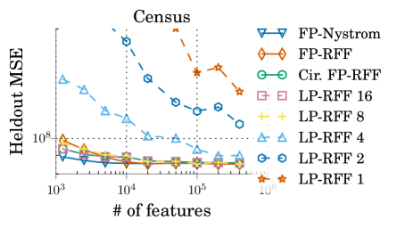
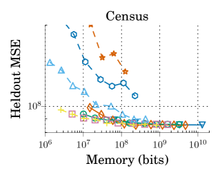
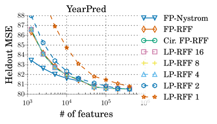
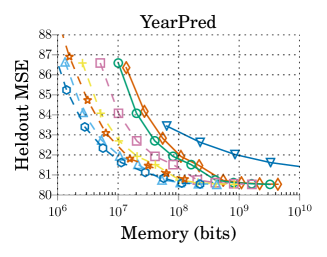
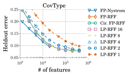
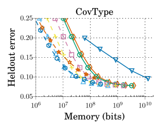
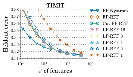
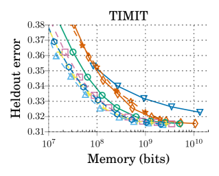
Figure 13: Generalization performance of the kernel approximation methods (Nyström, FP-RFFs, circ. FP-RFFs, LP-RFFs) with respect to the number of features used, as well as with respect to memory used. We observe that LP-RFFs demonstrate better generalization performance than the full-precision baselines under memory constraints, with 2-8 bits typically giving the best performance. Importantly, the relative ranking of the methods changes depending on whether we compare the methods based on their number of features, or their memory utilization. For example, the Nyström method shows better generalization performance than the RFF-based approaches with the same number of features. However, the Nyström method often performs significantly worse than the RFF methods under fixed memory budgets. We plot results averaged over three random seeds.

D.5 Empirical Evaluation of LP-RFFs (Section 5.1)

To empirically demonstrate the generalization performance of LP-RFFs, we compare LP-RFFs to FP-RFFs, circulant FP-RFFs, and Nyström features for various memory budgets. We use the same datasets as in Section 2, including Census and YearPred for regression, as well as CovType and TIMIT for classification. We use the same experimental protocol as in Section 2 (details in Appendix D.2), with the only significant additions being that we also evaluate the performance of circulant FP-RFFs, and LP-RFFs for precisions $b\in\{1,2,4,8,16\}$. As noted in the main text, all our LP-RFF experiments are done in simulation; in particular, we represent each low-precision feature as a 64-bit floating point number, whose value is one of the $2^{b}$ values representable in $b$ bits. For our full-precision experiments we also use 64-bit floats, but we report the memory utilization of these experiments as if we used 32 bits, to avoid inflating the relative gains of LP-RFFs over the full-precision approaches. We randomly sample the quantization noise for each mini-batch independently each epoch.

In Section 5.1 (Figure 4), we demonstrated the generalization performance of LP-RFFs on the TIMIT, YearPred, and CovType datasets, using 4 bits per feature. In Figure 13, we additionally include results on the Census dataset, and include results for a larger set of precisions ($b\in\{1,2,4,8,16\}$). We also include plots of heldout performance as a function of the number of features used. We observe that LP-RFFs, using 2-8 bits, systematically outperform the full-precision baselines under different memory budgets.

We run on four additional classification and regression datasets (Forest, Cod-RNA, Adult, CPU) to compare the empirical performance of LP-RFFs to full-precision RFFs, circulant RFFs and Nyström. We present the results in Figure 14, and observe that LP-RFFs can achieve competitive generalization performance to the full-precision baselines with lower training memory budgets. With these 4 additional datasets, our empirical evaluation of LP-RFFs now covers all the datasets investigated in Yang et al. (2012). We include details about these datasets and the hyperparameters we used in Tables 7 and 8.

Table 7: Dataset details for the additional datasets from Section D.5. For classification tasks, we write the number of classes in parentheses in the “Task” column.

Dataset	Task	Train	Heldout	Test	# Features
Forest	Class. (2)	470k	52k	58k	54
Cod-RNA	Class. (2)	54k	6k	272k	8
Adult	Class. (2)	29k	3k	16k	123
CPU	Reg.	6k	0.7k	0.8k	21

Table 8: The Gaussian kernel bandwidths used, and the search grid for initial learning rate on the Forest, Cod-RNA, Adult, and CPU datasets. Optimal learning rate in bold.

Dataset	$1/2\sigma^{2}$	Initial learning rate grid
Forest	0.5	5.0, 10.0, 50.0, 100.0, 500.0
Cod-RNA	0.4	10.0, 50.0, 100.0, 500.0, 1000.0
Adult	0.1	5.0, 10.0, 50.0, 100.0, 500.0, 1000.0
CPU	0.03	0.05, 0.1, 0.5, 1.0, 5.0

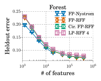
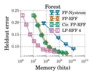
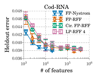
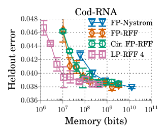
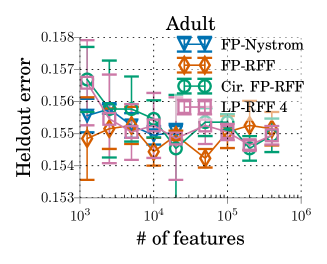
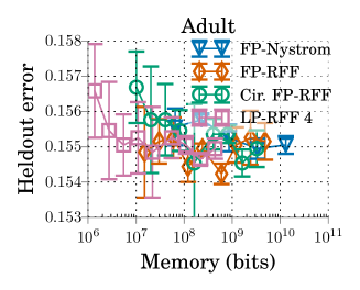
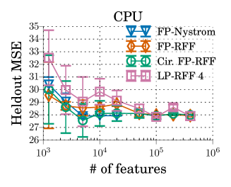
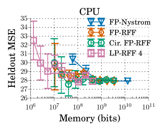
Figure 14: Comparison of the performance of LP-RFFs and the full-precision baselines on additional datasets, with respect to the number of features used, as well as with respect to memory used. We observe that LP-RFFs can achieve performance competitive with the full-precision baseline methods, with significant memory savings. We plot the average performance across three random seeds, with error bars indicating standard deviations.

D.6 Generalization Performance vs. $(\Delta_{1},\Delta_{2})$ (Section 5.2)

For our experiments in Section 5.2, we use the same protocol and hyperparameters (learning rate, $\lambda$) as for the $(\Delta_{1},\Delta_{2})$ experiments in Section 3.2. However, we additionally run experiments with LP-RFFs for precisions $b\in\{1,2,4,8,16\}$. We use five random seeds for each experimental setting, and plot the average results, with error bars indicating standard deviations.

In Figure 15, we plot an extended version of the right plots in Figure 5. We include results for all precisions, and for both Census and CovType. We observe that on Census, $1/(1-\Delta_{1})$ does not align well with performance (Spearman rank correlation coefficient $\rho=0.403$), because the low-precision features ($b=1$ or $b=2$) perform significantly worse than the full-precision features of the same dimensions. In this case, when we consider the impact of $\Delta_{2}$ by taking $\max\big{(}1/(1-\Delta_{1}),\Delta_{2}\big{)}$, we see that performance aligns much better ($\rho=0.959$).

On CovType, on the other hand, the impact on generalization performance from using low-precision is much less pronounced, so $1/(1-\Delta_{1})$ and $\max\big{(}1/(1-\Delta_{1}),\Delta_{2}\big{)}$ both align well with performance ($\rho=0.942$). Furthermore, in the case of CovType, $\Delta_{2}$ is generally smaller than $1/(1-\Delta_{1})$, so taking the $\max$ does not change the plot significantly.

To compute the Spearman rank correlation coefficients $\rho$ for these plots, we take the union of all the experiments which are a part of the plot. In particular, we include FP-RFFs, circulant FP-RFFs, FP-Nyström , and LP-RFFs with precisions $b\in\{1,2,4,8,16\}$. Although we plot the average performance across five random seeds in the plot, to compute $\rho$ we treat each experiment independently.

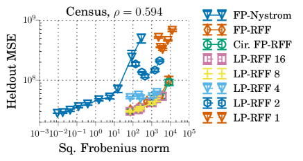
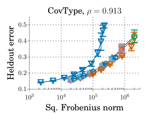
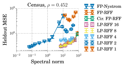
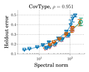
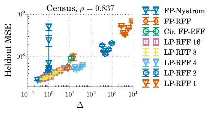
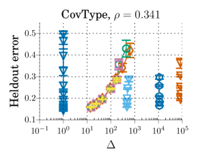
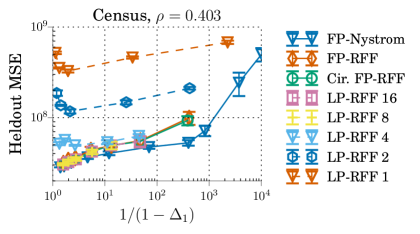
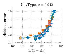
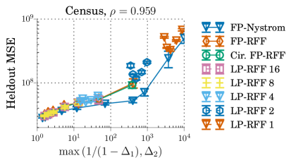
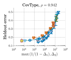
Figure 15: Generalization performance vs. different kernel approximation metrics on Census and CovType. The metric $\max\left(1/(1-\Delta_{1}),\Delta_{2}\right)$ is able to incorporate the influence of both $\Delta_{1}$ and $\Delta_{2}$ on performance for LP-RFFs, aligning well with generalization performance on both Census (Spearman rank correlation coefficient $\rho=0.959$) and CovType ($\rho=0.942$). $1/(1-\Delta_{1})$, on the other hand, fails to align well on Census ($\rho=0.403$), but does align on CovType ($\rho=0.942$). Note that although we plot the average performance across five random seeds for each experimental setting (error bars indicate standard deviation), when we compute the $\rho$ values we treat each experimental result independently (without averaging).

D.7 Other Experimental Results

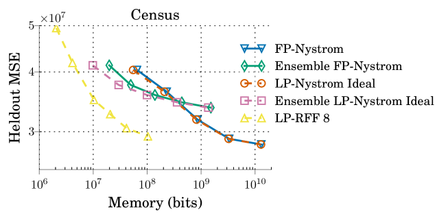
Figure 16: We plot the heldout performance (MSE) for the full-precision Nyström method, the ensemble Nyström method, and 8-bit LP-RFFs. We also show the best possible performance for the Nyström methods, assuming only the kernel approximation features are quantized (denoted “ideal”); we compute this by plotting the full-precision results but without counting the memory occupied by the features. The LP-RFF method significantly outperforms the “ideal” Nyström methods as a function of memory.

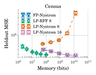
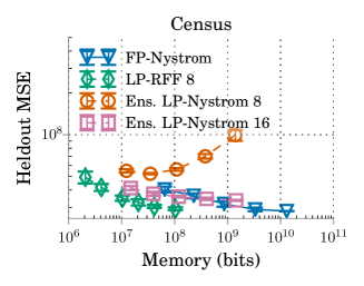
(a) LP-Nyström	(b) Ensemble LP-Nyström

Figure 17: The generalization performance of low-precision Nyström and low-precision ensemble Nyström, using a uniform quantization scheme.

D.7.1 Low-Precision Nyström

We encounter two main obstacles to attaining strong performance with the Nyström method under a memory budget: (1) For the standard Nyström method, because of the large projection matrix ($32m^{2}$ space), there are inherent limits to the memory savings attainable by only quantizing the features, regardless of the quantization scheme used. (2) While the ensemble Nyström method (Kumar et al., 2009) is a well-known method which can dramatically reduce the space occupied by the the Nyström projection matrix, it does not attain meaningful gains in performance under a memory budget. To demonstrate the first issue empirically, we plot in Figure 16 the performance of the full-precision Nyström methods without counting the memory from the feature mini-batches (denoted “ideal”). This is the best possible performance under any quantization scheme for these Nyström methods, assuming only the features are quantized. LP-RFFs still outperform these “ideal” methods for fixed memory budgets. To demonstrate the second issue, in Figure 16 we also plot the generalization performance of the ensemble method vs. the standard Nyström method, as a function of memory. We can see that the ensemble method does not attain meaningful gains over the standard Nyström method, as a function of memory.

Lastly, we mention that quantizing Nyström features is more challenging due to their larger dynamic range. For Nyström, all we know is that each feature is between $-1$ and $1$, whereas for RFFs, each feature is between $-\sqrt{2/m}$ and $\sqrt{2/m}$. In Figure 17 we plot our results quantizing Nyström features with the following simple scheme: for each feature, we find the maximum and minimum value on the training set, and then uniformly quantize this interval using $b$ bits. We observe that performance degrades significantly with less than or equal to 8 bits compared to full-precision Nyström. Although using the ensemble method reduces the dynamic range by a factor of $\sqrt{r}$ with $r$ blocks (we use $r=10$, a common setting in (Kumar et al., 2012)), and also saves space on the projection matrix, these strengths do not result in significantly better performance for fixed memory budgets.

D.7.2 Low-Precision Training for LP-RFFs

As discussed in Section 2.1, there are a number of ways to reduce the memory occupied by the model parameters, including (1) using a low-rank decomposition of the parameter matrix (Sainath et al., 2013a), (2) using structured matrices (Sindhwani et al., 2015), and (3) using low-precision (De Sa et al., 2018). Though these methods are orthogonal to our LP-RFF method, we now present results using a low-precision parameterization of the model, and show that we can attain similar performance to full-precision training. We use a training algorithm called LM-HALP (linear model high-accuracy low-precision) (De Sa et al., 2018). By parameterizing the model in low precision, this algorithm eliminates the need of casting the LP-RFFs back into full precision in order to multiply them with the model parameters. This approach also allows for these matrix multiplications to be implemented using fast low-precision matrix operations, and reduces the memory occupied by the model during training.

LM-HALP is based on the stochastic variance-reduced gradient (SVRG) algorithm. The model is parameterized using a low-precision fixed-point representation during training. In LM-HALP, all of the matrix multiplications involved in the stochastic model updates are done using low-precision fixed-point operations; however, the periodic computation of the full gradient is calculated in full precision (this is embarrassingly parallelizable). Importantly, even though most of training is done in low precision, the final model returned by this training algorithm is a full-precision model. We can further simplify the LM-HALP algorithm by replacing the SVRG updates with SGD updates, thus eliminating the need for calculating and storing the full gradient. In Figure 18 we present our results using LM-HALP on TIMIT, our largest and most challenging dataset; we use 8-bit LM-HALP (SVRG and SGD) on top of 8-bit LP-RFFs, and compare to full-precision SGD training. For LM-HALP based training, we perform the bit centering and rescaling operation after each training epoch. Under this setting, we show that when the number of features is at least $10,000$, the performance of both versions of HALP closely matches that of full-precision training.

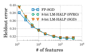
Figure 18: Low-precision vs. full-precision training algorithms on TIMIT using 8-bit LP-RFFs.

D.7.3 Double Sampling

We perform some initial experiments using the double sampling method of Zhang et al. (2017). In particular, we use a different random quantization of the LP-RFFs on the “forward pass” of our algorithm than in the “backward pass.” In our initial experiments with double sampling, as shown in Figure 19, we did not observe noticeable improvements in performance. These experiments were on the YearPred dataset with the Gaussian kernel. We leave a more extended investigation of these gradient bias reduction methods for future work.

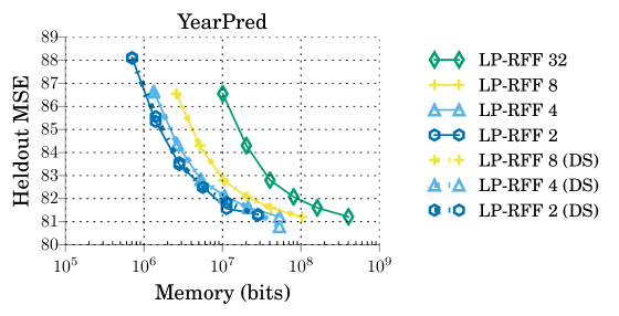
Figure 19: Comparison of LP-RFFs with and without double sampling on the YearPred dataset.

Appendix E EXTENDED RELATED WORK

Generalization Performance of Kernel Approximation Methods

From a theoretical perspective, there has been a lot of work analyzing the generalization performance of kernel approximation methods (Rahimi and Recht, 2008; Cortes et al., 2010; Sutherland and Schneider, 2015; Rudi and Rosasco, 2017; Avron et al., 2017; Li et al., 2018). The work most relevant to ours is that of Avron et al. (2017), which defines $\Delta$-spectral approximation and bounds the generalization performance of kernel approximation methods in terms of $\Delta$. This approach differs from works which evaluate kernel approximation methods in terms of the Frobenius or spectral norms of their kernel approximation matrices (Cortes et al., 2010; Gittens and Mahoney, 2016; Yang et al., 2014; Sutherland and Schneider, 2015; Yu et al., 2016; Dao et al., 2017). Our work shows the promise of Avron et al.’s approach, and builds upon it.

Large-Scale Kernel Experiments

On the topic of scaling kernel methods to large datasets, there have been a few notable recent papers. Tu et al. (2016) propose a distributed block coordinate descent method for solving large-scale least squares problems using the Nyström method or RFFs. The recent work of May et al. (2017) uses a single GPU to train large RFF models on speech recognition datasets, showing comparable performance to fully-connected deep neural networks. That work was limited by the number of features that could fit on a single GPU, and thus our proposed method could help scale these results.

References

• Alaoui and Mahoney (2015) Ahmed El Alaoui and Michael W. Mahoney. Fast randomized kernel ridge regression with statistical guarantees. In NIPS, pages 775–783, 2015.
• Avron et al. (2017) Haim Avron, Michael Kapralov, Cameron Musco, Christopher Musco, Ameya Velingker, and Amir Zandieh. Random Fourier features for kernel ridge regression: Approximation bounds and statistical guarantees. In ICML, volume 70 of Proceedings of Machine Learning Research, pages 253–262. PMLR, 2017.
• Caulfield et al. (2017) Adrian M. Caulfield, Eric S. Chung, Andrew Putnam, Hari Angepat, Daniel Firestone, Jeremy Fowers, Michael Haselman, Stephen Heil, Matt Humphrey, Puneet Kaur, Joo-Young Kim, Daniel Lo, Todd Massengill, Kalin Ovtcharov, Michael Papamichael, Lisa Woods, Sitaram Lanka, Derek Chiou, and Doug Burger. Configurable clouds. IEEE Micro, 37(3):52–61, 2017.
• Chen et al. (2016) Jie Chen, Lingfei Wu, Kartik Audhkhasi, Brian Kingsbury, and Bhuvana Ramabhadrari. Efficient one-vs-one kernel ridge regression for speech recognition. In ICASSP, pages 2454–2458. IEEE, 2016.
• Cortes et al. (2010) Corinna Cortes, Mehryar Mohri, and Ameet Talwalkar. On the impact of kernel approximation on learning accuracy. In AISTATS, volume 9 of JMLR Proceedings, pages 113–120. JMLR.org, 2010.
• Dao et al. (2017) Tri Dao, Christopher De Sa, and Christopher Ré. Gaussian quadrature for kernel features. In NIPS, pages 6109–6119, 2017.
• De Sa et al. (2015) Christopher De Sa, Ce Zhang, Kunle Olukotun, and Christopher Ré. Taming the wild: A unified analysis of Hogwild-style algorithms. In NIPS, pages 2674–2682, 2015.
• De Sa et al. (2017) Christopher De Sa, Matthew Feldman, Christopher Ré, and Kunle Olukotun. Understanding and optimizing asynchronous low-precision stochastic gradient descent. In ISCA, pages 561–574. ACM, 2017.
• De Sa et al. (2018) Christopher De Sa, Megan Leszczynski, Jian Zhang, Alana Marzoev, Christopher R. Aberger, Kunle Olukotun, and Christopher Ré. High-accuracy low-precision training. arXiv preprint arXiv:1803.03383, 2018.
• Dheeru and Karra Taniskidou (2017) Dua Dheeru and Efi Karra Taniskidou. UCI machine learning repository, 2017.
• Gales (1998) M. J. F. Gales. Maximum likelihood linear transformations for HMM-based speech recognition. Computer Speech & Language, 12(2):75–98, 1998.
• Garofolo et al. (1993) J. S. Garofolo, L. F. Lamel, W. M. Fisher, J. G. Fiscus, D. S. Pallett, and N. L. Dahlgren. DARPA TIMIT acoustic phonetic continuous speech corpus CDROM, 1993. URL http://www.ldc.upenn.edu/Catalog/LDC93S1.html.
• Gittens and Mahoney (2016) Alex Gittens and Michael W. Mahoney. Revisiting the Nyström method for improved large-scale machine learning. Journal of Machine Learning Research, 17:117:1–117:65, 2016.
• Gupta et al. (2015) Suyog Gupta, Ankur Agrawal, Kailash Gopalakrishnan, and Pritish Narayanan. Deep learning with limited numerical precision. In ICML, volume 37 of JMLR Workshop and Conference Proceedings, pages 1737–1746, 2015.
• Han et al. (2016) Song Han, Huizi Mao, and William J. Dally. Deep compression: Compressing deep neural network with pruning, trained quantization and Huffman coding. In Proceedings of the International Conference on Learning Representations (ICLR), 2016.
• Hsieh et al. (2014) Cho-Jui Hsieh, Si Si, and Inderjit S. Dhillon. Fast prediction for large-scale kernel machines. In NIPS, pages 3689–3697, 2014.
• Huang et al. (2014) Po-Sen Huang, Haim Avron, Tara N. Sainath, Vikas Sindhwani, and Bhuvana Ramabhadran. Kernel methods match deep neural networks on TIMIT. In ICASSP, pages 205–209. IEEE, 2014.
• Hubara et al. (2016) Itay Hubara, Matthieu Courbariaux, Daniel Soudry, Ran El-Yaniv, and Yoshua Bengio. Binarized neural networks. In NIPS, pages 4107–4115, 2016.
• Jouppi et al. (2017) Norman P. Jouppi, Cliff Young, Nishant Patil, David A. Patterson, et al. In-datacenter performance analysis of a tensor processing unit. In ISCA, pages 1–12. ACM, 2017.
• Kumar et al. (2009) Sanjiv Kumar, Mehryar Mohri, and Ameet Talwalkar. Ensemble Nyström method. In NIPS, pages 1060–1068, 2009.
• Kumar et al. (2012) Sanjiv Kumar, Mehryar Mohri, and Ameet Talwalkar. Sampling methods for the Nyström method. Journal of Machine Learning Research, 13:981–1006, 2012.
• Le et al. (2013) Quoc V. Le, Tamás Sarlós, and Alexander J. Smola. Fastfood - computing Hilbert space expansions in loglinear time. In ICML, volume 28 of JMLR Workshop and Conference Proceedings, pages 244–252, 2013.
• Li et al. (2018) Zhu Li, Jean-Francois Ton, Dino Oglic, and Dino Sejdinovic. A unified analysis of random Fourier features. arXiv preprint arXiv:1806.09178, 2018.
• May (2018) Avner May. Kernel Approximation Methods for Speech Recognition. PhD thesis, Columbia University, 2018.
• May et al. (2016) Avner May, Michael Collins, Daniel J. Hsu, and Brian Kingsbury. Compact kernel models for acoustic modeling via random feature selection. In ICASSP, pages 2424–2428. IEEE, 2016.
• May et al. (2017) Avner May, Alireza Bagheri Garakani, Zhiyun Lu, Dong Guo, Kuan Liu, Aurélien Bellet, Linxi Fan, Michael Collins, Daniel J. Hsu, Brian Kingsbury, Michael Picheny, and Fei Sha. Kernel approximation methods for speech recognition. arXiv preprint arXiv:1701.03577, 2017.
• Morgan and Bourlard (1990) N. Morgan and H. Bourlard. Generalization and parameter estimation in feedforward nets: Some experiments. In NIPS, 1990.
• Musco and Musco (2017) Cameron Musco and Christopher Musco. Recursive sampling for the Nyström method. In NIPS, pages 3836–3848, 2017.
• Nemirovski et al. (2009) Arkadi Nemirovski, Anatoli Juditsky, Guanghui Lan, and Alexander Shapiro. Robust stochastic approximation approach to stochastic programming. SIAM Journal on Optimization, 19(4):1574–1609, 2009.
• Popoviciu (1935) Tiberiu Popoviciu. Sur les équations algébriques ayant toutes leurs racines réelles. Mathematica, 9:129–145, 1935.
• Rahimi and Recht (2007) Ali Rahimi and Benjamin Recht. Random features for large-scale kernel machines. In NIPS, pages 1177–1184, 2007.
• Rahimi and Recht (2008) Ali Rahimi and Benjamin Recht. Weighted sums of random kitchen sinks: Replacing minimization with randomization in learning. In NIPS, pages 1313–1320, 2008.
• Rudi and Rosasco (2017) Alessandro Rudi and Lorenzo Rosasco. Generalization properties of learning with random features. In NIPS, pages 3218–3228, 2017.
• Sainath et al. (2013a) Tara N. Sainath, Brian Kingsbury, Vikas Sindhwani, Ebru Arisoy, and Bhuvana Ramabhadran. Low-rank matrix factorization for deep neural network training with high-dimensional output targets. In ICASSP, pages 6655–6659. IEEE, 2013a.
• Sainath et al. (2013b) Tara N. Sainath, Brian Kingsbury, Hagen Soltau, and Bhuvana Ramabhadran. Optimization techniques to improve training speed of deep neural networks for large speech tasks. IEEE Trans. Audio, Speech & Language Processing, 21(11):2267–2276, 2013b.
• Si et al. (2014) Si Si, Cho-Jui Hsieh, and Inderjit S. Dhillon. Memory efficient kernel approximation. In ICML, volume 32 of JMLR Workshop and Conference Proceedings, pages 701–709, 2014.
• Sindhwani et al. (2015) Vikas Sindhwani, Tara N. Sainath, and Sanjiv Kumar. Structured transforms for small-footprint deep learning. In NIPS, pages 3088–3096, 2015.
• Sutherland and Schneider (2015) Dougal J. Sutherland and Jeff G. Schneider. On the error of random Fourier features. In UAI, pages 862–871. AUAI Press, 2015.
• Tropp (2015) Joel A. Tropp. An introduction to matrix concentration inequalities. Foundations and Trends in Machine Learning, 8(1-2):1–230, 2015.
• Tu et al. (2016) Stephen Tu, Rebecca Roelofs, Shivaram Venkataraman, and Benjamin Recht. Large scale kernel learning using block coordinate descent. arXiv preprint arXiv:1602.05310, 2016.
• Wei et al. (2017) Yuting Wei, Fanny Yang, and Martin J. Wainwright. Early stopping for kernel boosting algorithms: A general analysis with localized complexities. In NIPS, pages 6067–6077, 2017.
• Williams and Seeger (2000) Christopher K. I. Williams and Matthias W. Seeger. Using the Nyström method to speed up kernel machines. In NIPS, pages 682–688. MIT Press, 2000.
• Yang et al. (2014) Jiyan Yang, Vikas Sindhwani, Haim Avron, and Michael W. Mahoney. Quasi-Monte Carlo feature maps for shift-invariant kernels. In Proceedings of the 31th International Conference on Machine Learning, ICML 2014, Beijing, China, 21-26 June 2014, pages 485–493, 2014.
• Yang et al. (2012) Tianbao Yang, Yu-Feng Li, Mehrdad Mahdavi, Rong Jin, and Zhi-Hua Zhou. Nyström method vs random Fourier features: A theoretical and empirical comparison. In NIPS, pages 485–493, 2012.
• Yang et al. (2015) Zichao Yang, Marcin Moczulski, Misha Denil, Nando de Freitas, Alexander J. Smola, Le Song, and Ziyu Wang. Deep fried convnets. In ICCV, pages 1476–1483. IEEE Computer Society, 2015.
• Yen et al. (2014) Ian En-Hsu Yen, Ting-Wei Lin, Shou-De Lin, Pradeep Ravikumar, and Inderjit S. Dhillon. Sparse random feature algorithm as coordinate descent in Hilbert space. In NIPS, pages 2456–2464, 2014.
• Yu et al. (2015) Felix X. Yu, Sanjiv Kumar, Henry A. Rowley, and Shih-Fu Chang. Compact nonlinear maps and circulant extensions. arXiv preprint arXiv:1503.03893, 2015.
• Yu et al. (2016) Felix X. Yu, Ananda Theertha Suresh, Krzysztof Marcin Choromanski, Daniel N. Holtmann-Rice, and Sanjiv Kumar. Orthogonal random features. In NIPS, pages 1975–1983, 2016.
• Zhang et al. (2017) Hantian Zhang, Jerry Li, Kaan Kara, Dan Alistarh, Ji Liu, and Ce Zhang. Zipml: Training linear models with end-to-end low precision, and a little bit of deep learning. In ICML, volume 70 of Proceedings of Machine Learning Research, pages 4035–4043. PMLR, 2017.
• Zhang et al. (2005) Tong Zhang, Bin Yu, et al. Boosting with early stopping: Convergence and consistency. The Annals of Statistics, 33(4):1538–1579, 2005.