Distribution of complex algebraic numbers
on the unit circle

Abstract.

For $-\pi\leq\beta_{1}<\beta_{2}\leq\pi$ denote by $\Phi_{\beta_{1},\beta_{2}}(Q)$ the number of algebraic numbers on the unit circle with arguments in $[\beta_{1},\beta_{2}]$ of degree $2m$ and with elliptic height at most $Q$. We show that

$$\Phi_{\beta_{1},\beta_{2}}(Q)=Q^{m+1}\int\limits_{\beta_{1}}^{\beta_{2}}{p(t)}\,{\rm d}t+O\left(Q^{m}\,\log Q\right),\quad Q\to\infty,$$

where $p(t)$ coincides up to a constant factor with the density of the roots of some random trigonometric polynomial. This density is calculated explicitly using the Edelman–Kostlan formula.

1. Introduction

The problem of distribution of real and complex algebraic numbers has been studied intensively in the last two decades and turned out to be closely related with the distribution of roots of random polynomials. We first give a brief review of recent results in this area before describing the problem considered in this paper.

Let $\mathbb{A}$ denote the field of (all) algebraic numbers over $\mathbb{Q}$ and let $\mathbb{A}_{n}$ denote the set of algebraic numbers of degree $n\in\mathbb{N}$. Note that the set $\mathbb{A}_{n}$ is countable and any open subset of $\mathbb{R}$ or $\mathbb{C}$ contains already infinitely many algebraic numbers. In order to study the distribution of those algebraic numbers, we need to select finite (ordered) subsets of $\mathbb{A}_{n}$. To this end, we consider a height function $h:\mathbb{A}\to\mathbb{R}_{+}$ such that for any $n\in\mathbb{N}$ and $Q>0$ there are only finitely many algebraic numbers $\alpha$ of degree $n$ with $h(\alpha)\leq Q$. Note that one usually requires (which we will always assume) that $h(\alpha^{\prime})=h(\alpha)$ for all conjugates of $\alpha$.

A natural question is to determine the asymptotics of the number of $\alpha\in\mathbb{A}_{n}$ lying in a given subset of $\mathbb{R}$ or $\mathbb{C}$ such that $h(\alpha)\leq Q$ and degree $n$ is fixed as $Q\to\infty$. This problem has been studied by Masser and Vaaler [11] with height function being the Mahler measure. Later Koleda [9] determined the asymptotic number of real algebraic numbers ordered by the naïve height; the same result for complex algebraic numbers was obtained in [7]. A generalization of the naïve height, the weighted $l_{p}$-norm (which also generalizes the length, the Euclidean norm, and the Bombieri $p$-norm), was considered in [8]. Another interesting example of heights – namely the house of an algebraic number – was studied in [2], which studies the distribution of Perron numbers.

In the present note we would like to study the distribution of algebraic numbers on the unit circle. Although our methods work for any weighted $l_{p}$-norm (including the naïve height), we consider the weighted Euclidean (or elliptic) height only: this case corresponds to the simplest asymptotic distribution formula.

The paper is organized as follows. In the next section, we formulate our main result Theorem 2.1 and give some corollaries. The proof of Theorem 2.1 is given in Section 3. Section 4 contains the proof of some auxiliary statements and the corollaries are proved in Section  5.

2. Basic notation and main result

Given a polynomial $P(t):=a_{n}t^{n}+\ldots+a_{1}t+a_{0}$ and a vector of positive weights $\mathbf{\lambda}=(\lambda_{0},\lambda_{1},\dots,\lambda_{n})$ define the elliptic height of $P$ as

$$h_{\mathbf{\lambda}}(P):=\left(\sum\limits_{k=0}^{n}\frac{a_{k}^{2}}{\lambda_{k}^{2}}\right)^{1/2}.$$

Let $\mathcal{P}(Q)$ denote the class of integral polynomials (that is, with integer coefficients) of degree $n$ and with height $h_{\mathbf{\lambda}}$ at most $Q$:

$$\mathcal{P}(Q):=\{P\in\mathbb{Z}[t]\colon\deg P=n,\,h_{\mathbf{\lambda}}(P)\leq Q\}.$$

We say that an integral polynomial is prime, if it is irreducible over $\mathbb{Q}$, primitive (with co-prime coefficients), and its leading coefficient is positive. Denote by $\mathcal{P}^{*}(Q)$ the class of prime polynomials from $\mathcal{P}(Q)$:

$$\mathcal{P}^{*}(Q):=\{P\in\mathcal{P}(Q)\colon P\text{ is prime}\}.$$

The minimal polynomial of an algebraic number $\alpha$ is the uniquely defined prime polynomial $P\in\mathbb{Z}[t]$ satisfying $P(\alpha)=0$. Then, the elliptic height of $\alpha$ is defined as the elliptic height of its minimal polynomial:

$$h_{\mathbf{\lambda}}(\alpha):=h_{\mathbf{\lambda}}(P).$$

The other roots of $P$ are called algebraic conjugates of $\alpha$.

We aim to investigate the asymptotic behavior of the algebraic numbers on the unit circle $\mathbb{T}\subset\mathbb{C}$:

$$\mathbb{T}:=\{z\in\mathbb{C}:|z|=1\}.$$

We start with the simple observation that any algebraic number on $\mathbb{T}$ has even degree and the coefficients of its minimal polynomial posses some symmetry property. Indeed, consider an algebraic number $\alpha\in\mathbb{T}$ with the minimal polynomial

$$P(t)=a_{n}t^{n}+\ldots+a_{1}t+a_{0}.$$

Since the coefficients of $P$ are real, $\bar{\alpha}$ is also a root of $P$. Moreover, $\alpha\in\mathbb{T}$ implies $\bar{\alpha}=1/\alpha$. Thus,

$$P(\alpha)=P\left(\frac{1}{\alpha}\right)=0,$$

which means that $\alpha$ is a root of the polynomial

$$\tilde{P}(t):=t^{n}P(t^{-1})=a_{0}t^{n}+\ldots+a_{n-1}t+a_{n}.$$

Hence, by definition of minimal polynomial we conclude that $P$ is a multiple of $\tilde{P}$ which leaves us with two possibilities only: $P\equiv-\tilde{P}$ or $P\equiv\tilde{P}$. The former one would imply that $1$ is a root of $P$ which is impossible due to its irreducibility. Therefore $P\equiv\tilde{P}$ which means

$$a_{k}=a_{n-k},\quad 0\leq k\leq n.$$

For odd $n$, this condition implies that $-1$ is a root of $P$ which, again, contradicts with its irreducibility. Thus from now on we consider only algebraic numbers of even degree

$$n=2m,\quad m\geq 1.$$

The number $m$ will stay throughout the paper.

Now we are ready to formulate our main result. For

$$-\pi\leq\beta_{1}<\beta_{2}\leq\pi$$ (1)

denote by $\Phi_{\beta_{1},\beta_{2}}(Q)$ the number of algebraic numbers of degree $n=2m$ on the unit circle with arguments in $[\beta_{1},\beta_{2}]$ and with elliptic height at most $Q$:

$$\Phi_{\beta_{1},\beta_{2}}(Q):=\#\left\{\theta\in[\beta_{1},\beta_{2}]\colon e^{i\theta}\in\mathbb{A}_{2m},h_{\mathbf{\lambda}}\left(e^{i\theta}\right)\leq Q\right\}.$$

Denote by $\zeta(\cdot)$ the Riemann zeta function and by $\mathbb{B}^{m+1}$ the $(m+1)$-dimensional unit ball of volume $\mathop{\mathrm{Vol}}\nolimits(\mathbb{B}^{m+1})$.

Theorem 2.1.

For any fixed symmetric vector of positive weights $\mathbf{\lambda}=(\lambda_{0},\dots,\lambda_{m},\dots,\lambda_{0})$ we have

$$\Phi_{\beta_{1},\beta_{2}}(Q)=\frac{\mathop{\mathrm{Vol}}\nolimits(\mathbb{B}^{m+1})}{2^{m/2+1}\pi\zeta(m+1)}\lambda_{0}\dots\lambda_{m}Q^{m+1}\int\limits_{\beta_{1}}^{\beta_{2}}{p_{\mathbf{\lambda}}(t)}\,{\rm d}t+O\left(Q^{m}\,\log Q\right),\quad Q\to\infty,$$

where

$$p_{\mathbf{\lambda}}(t):=\left[\frac{\partial^{2}}{\partial x\partial y}\log\left(\frac{\lambda_{m}^{2}}{2}+\sum\limits_{k=1}^{m}\lambda_{m-k}^{2}\,\cos(kx)\cos(ky)\right)\Big{|}_{x=y=t}\right]^{1/2}.$$ (2)

The implicit constant depends on $\mathbf{\lambda}$ and $m$ only and the $\log Q$ factor can be omitted for $m\geq 3$.

In this general form, the limit density $p_{\mathbf{\lambda}}$ is difficult to analyze. However, there are some examples of $\lambda$ where (2) can be simplified. The first one is the vector of Bombieri 2-norm weights.

Corollary 2.2.

For $\lambda_{k}=\sqrt{\binom{2m}{k}},k=0,\dots,2m,$ we have

$$p_{\mathbf{\lambda}}(t)=\sqrt{\frac{m}{2}}\cdot\frac{\left|\sin t\right|\,\sqrt{\sum\limits_{k=0}^{2m-2}\left(\cos t\right)^{2k}+(2m-1)\left(\cos t\right)^{2m-2}}}{\left(\cos t\right)^{2m}+1}.$$

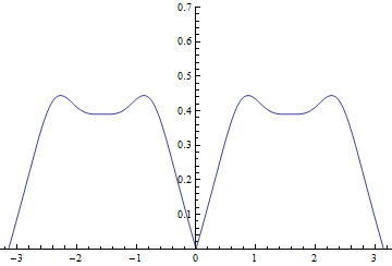
a

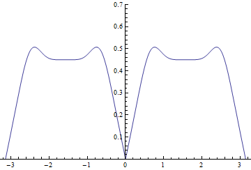
b

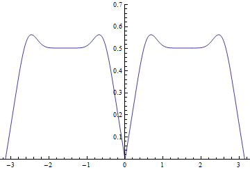
c

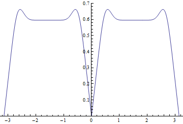
d

Figure 1. A plot of $p_{\mathbf{\lambda}}(t)$ with $\mathbf{\lambda}=\left(\binom{2m}{k}^{1/2}\right)_{k=0}^{n}$: a) $m=3$; b) $m=4$; c) $m=5$; d) $m=7$.

The second example is the Euclidean height.

Corollary 2.3.

For $\mathbf{\lambda}=\left(1,\ldots,1\right)$ we have

$$p_{\mathbf{\lambda}}(t) =\left(b_{m}+\frac{\sin(b_{m}t)}{\sin t}\right)^{-1}\cdot\Big{(}\frac{b_{m}\sin(b_{m}t)}{2(\sin t)^{3}}-\frac{b_{m}^{2}}{2}\frac{\cos(b_{m}t)\cos t}{(\sin t)^{2}}$$

$$+\frac{\left(\sin(b_{m}t)\right)^{2}}{4(\sin t)^{4}}-\frac{b_{m}^{3}+2b_{m}}{6}\frac{\sin(b_{m}t)}{\sin t}-\frac{b_{m}^{2}}{4(\sin t)^{2}}+\frac{(m^{2}+m)b_{m}^{2}}{3}\Big{)}^{1/2},$$

where $b_{m}=2m+1$.

a

b

c

d

Figure 2. A plot of $p_{\mathbf{\lambda}}(t)$ with $\mathbf{\lambda}=\left(1,\ldots,1\right)$: a) $m=3$; b) $m=4$; c) $m=5$; d) $m=7$.

As was mentioned above, the results on the distribution of the roots of random algebraic polynomials were used in [7], [8] to study the asymptotic behavior of algebraic numbers in a domain of the complex plane. In this paper we show that the distribution of algebraic numbers on the unit circle can be described in terms of random trigonometric polynomials. Namely, one can easily see from the proof of Theorem 2.1 that

$$\mathbb{E}\,\mu_{F}([\beta_{1},\beta_{2}])=\frac{1}{\pi}\int\limits_{\beta_{1}}^{\beta_{2}}\rho_{\lambda}(t){\rm d}t,$$

where

$$F(\theta):=\frac{\lambda_{m}}{2}\eta_{m}+\frac{1}{\sqrt{2}}\sum\limits_{k=1}^{m}\lambda_{m-k}\eta_{m-k}\,\cos(k\theta)$$

is a random trigonometric polynomial with coefficients $\eta_{0},\ldots,\eta_{m}$ being i.i.d. real-valued standard Gaussian variables and $\mu_{F}([\beta_{1},\beta_{2}])$ denotes the number of the real roots of $F$ lying in the interval $[\beta_{1},\beta_{2}]$. Thus, up to a factor $\pi$, the limit density $p_{\mathbf{\lambda}}$ coincides with the density of the roots of $F$.

3. Proof of Theorem 2.1

As argued in Section 2 we can restrict our attention to the following subclass of symmetric polynomials of even degree $n=2m$:

$$\mathcal{P}_{\mathrm{sym}}(Q):=\bigg{\{}P\in\mathcal{P}(Q)\colon P(t)=\sum\limits_{k=0}^{2m}a_{k}t^{k},\,a_{k}=a_{2m-k}\bigg{\}}.$$

Moreover let $\mathcal{P}^{*}_{\mathrm{sym}}(Q)$ denote the subclass of prime polynomials from $\mathcal{P}_{\mathrm{sym}}(Q)$:

$$\mathcal{P}^{*}_{\mathrm{sym}}(Q):=\mathcal{P}_{\mathrm{sym}}(Q)\cap\mathcal{P}^{*}(Q).$$

Given a function $g:\mathbb{C}\rightarrow\mathbb{C}$ and a subset $B\subset\mathbb{C}$ denote by $\mu_{g}(B)$ the number of the roots of $g$ lying in $B$. For $-\pi\leq\beta_{1}<\beta_{2}\leq\pi$ denote by $\mathbb{T}_{\beta_{1},\beta_{2}}$ the arc

$$\mathbb{T}_{\beta_{1},\beta_{2}}:=\left\{z\in\mathbb{T}\colon\arg z\in[\beta_{1},\beta_{2}]\right\}.$$

Since $\mathcal{P}_{\mathrm{sym}}^{*}(Q)$ is the set of all minimal polynomials for algebraic numbers $\alpha\in\mathbb{T}$ with $\deg\alpha=2m$ and $h_{\mathbf{\lambda}}\left(\alpha\right)\leq Q$, we have

$$\Phi_{\beta_{1},\beta_{2}}(Q)=\sum\limits_{P\in\mathcal{P}_{\mathrm{sym}}^{*}(Q)}\mu_{P}(\mathbb{T}_{\beta_{1},\beta_{2}})$$

and since $\mu_{P}(\mathbb{T}_{\beta_{1},\beta_{2}})\leq 2m$, we can write

$$\Phi_{\beta_{1},\beta_{2}}(Q)=\sum\limits_{l=0}^{2m}l\,\#\{P\in\mathcal{P}_{\mathrm{sym}}^{*}(Q):\,\mu_{P}(\mathbb{T}_{\beta_{1},\beta_{2}})=l\}.$$ (3)

Thus our aim is to estimate the number of the prime symmetric polynomials having a prescribed number of roots in a given set. Since these polynomials can be identified with the vectors of their coefficients, our first step is to find a way of counting integer points in multidimensional regions.

For a Borel set $A\subset\mathbb{R}^{d}$ denote by $\gamma(A)$ (resp. $\gamma^{*}(A)$) the number of points in $A$ with integer (resp. co-prime integer) coordinates. For a real number $r$ define the dilated set

$$rA:=\{r\mathbf{x}:\mathbf{x}\in A\}.$$

For our purposes we would like to know the asymptotic behavior of the quantity $\gamma^{*}(QA)$ as $Q\rightarrow\infty$. In order to get a good estimate one should impose some regularity conditions on the boundary $\partial A$ of $A$. According to [15, Definition 2.2], we say that $\partial A\subset\mathbb{R}^{d}$ is of Lipschitz class $(M,L)$ if there exist $M$ maps $\phi_{1},\dots,\phi_{M}:[0,1]^{d-1}\to\mathbb{R}^{d}$ satisfying a Lipschitz condition

$$|\phi_{i}(x)-\phi_{i}(y)|\leq L|x-y|\text{ for }x,y\in[0,1]^{d-1},\quad i=1,\dots,M,$$

such that $\partial A$ is covered by the images of the maps $\phi_{i}$.

The next lemma provides the asymptotic of $\gamma^{*}(QA)$ as $Q\rightarrow\infty$.

Lemma 3.1.

Consider a bounded region $A\subset\mathbb{R}^{d}$, $d\geq 2$, such that the boundary $\partial A$ of $A$ is of Lipschitz class $(M,L)$. Then $A$ is Lebesgue measurable and

$$\left|\frac{\lambda^{*}(QA)}{Q^{d}}-\frac{\mathop{\mathrm{Vol}}\nolimits(A)}{\zeta(d)}\right|\leq C\frac{\log^{\chi(d)}Q}{Q},$$

where $C$ depends on $d,L,M$ only and

$$\chi(d):=\left\{\begin{array}[]{ll}1,&d=2;\\ 0,&\text{otherwise}.\end{array}\right.$$ (4)

Proof.

See, e.g., [8, Lemma 6.3]. ∎

For $l=0,1,\dots,2m$ denote by $A_{l}\subset\mathbb{R}^{m+1}$ the set of points $(a_{0},\ldots,a_{m})$ such that the polynomial $P(t)=a_{0}t^{2m}+\ldots+a_{m}t^{m}+\ldots+a_{0}$ satisfies $\mu_{P}(\mathbb{T}_{\beta_{1},\beta_{2}})=l$ and $h_{\mathbf{\lambda}}\left(P\right)\leq 1$. The latter condition is equivalent to $(a_{0},\ldots,a_{m})\in\mathcal{E}_{\mathbf{\lambda}}$, where $\mathcal{E}_{\mathbf{\lambda}}\subset\mathbb{R}^{m+1}$ is the ellipsoid defined by

$$\mathcal{E}_{\mathbf{\lambda}}:=\bigg{\{}(a_{0},\ldots,a_{m})\in\mathbb{R}^{m+1}:\frac{a_{m}^{2}}{\lambda_{m}^{2}}+2\sum\limits_{k=0}^{m-1}\frac{a_{k}^{2}}{\lambda_{k}^{2}}\leq 1\bigg{\}}.$$

Note that

$$\mathop{\mathrm{Vol}}\nolimits(\mathcal{E}_{\mathbf{\lambda}})=2^{-m/2}\lambda_{0}\dots\lambda_{m}\mathop{\mathrm{Vol}}\nolimits(\mathbb{B}^{m+1}).$$

Then by definition of a primitive polynomial we have

$$\gamma^{*}(QA_{l})=\#\{P\in\mathcal{P}_{\mathrm{sym}}(Q):P\text{ is primitive},\,\mu_{P}(\mathbb{T}_{\beta_{1},\beta_{2}})=l\},$$

which implies

$$\Big{|}\frac{1}{2}\,\gamma^{*}(Q\,A_{l})-\#\{P\in\mathcal{P}_{\mathrm{sym}}^{*}(Q):\,\mu_{P}(\mathbb{T}_{\beta_{1},\beta_{2}})=l\}\Big{|}\leq r(Q).$$ (5)

Here, $r(Q)$ denotes the number of the polynomials reducible in $\mathcal{P}_{\mathrm{sym}}(Q)$ (i.e., can be represented as a product of two symmetric integral polynomials of positive degree). The factor $1/2$ in (5) is due to the positiveness of the leading coefficient of a prime polynomial.

Thus, our next step is to estimate $\gamma^{*}(Q\,A_{l})$ and $r(Q)$. The latter is established in the following lemma.

Lemma 3.2.

For some $C>0$ depending on $m,\lambda$ only we have

$$r(Q)\leq C\cdot Q^{m}\,\log^{\chi(m)}Q,$$

where $\chi(\cdot)$ is defined in (4).

The proof of Lemma 3.2 is postponed to Section 4. In order to estimate $\gamma^{*}(Q\,A_{l})$, we are going to apply Lemma 3.1. Before we do it, we need to check that the boundary of $A_{l}$ is of Lipschitz class.

Lemma 3.3.

For any $0\leq l\leq m$, there exist constants $M$, $L$ depending on $m,\mathbf{\lambda}$ only such that the boundary $\partial A_{l}$ is of Lipschitz class $(M,L)$.

This lemma is a slightly modified and simplified version of [8, Lemma 6.4]. For the reader’s convenience, we give a detailed proof of Lemma 3.3 in Section 4.

Now taking Lemma 3.3 into account we can apply Lemma 3.1 to the set $A_{l}$ which together with (5) and Lemma 3.2 gives

$$\#\{P\in\mathcal{P}_{\mathrm{sym}}^{*}(Q):\,\mu_{P}\left(\mathbb{T}_{\beta_{1},\beta_{2}}\right)=l\}=\frac{\mathop{\mathrm{Vol}}\nolimits(A_{l})}{2\zeta(m+1)}\,Q^{m+1}+O\left(Q^{m}\,\log^{\chi(m)}Q\right),$$

and, due to (3), we conclude that

$$\Phi_{\beta_{1},\beta_{2}}(Q)=\frac{Q^{m+1}}{2\zeta(m+1)}\,\sum\limits_{l=0}^{2m}l\,\mathop{\mathrm{Vol}}\nolimits(A_{l})+O\left(Q^{m}\,\log^{\chi(m)}Q\right).$$ (6)

To compute the sum on the right-hand side of (6) consider the random polynomial

$$G(z):=\sum_{k=0}^{m-1}\xi_{k}(z^{k}+z^{2m-k})+\xi_{m}z^{m},$$

where the random vector

$$\left(\frac{\xi_{0}}{\lambda_{0}/\sqrt{2}},\dots,\frac{\xi_{m-1}}{\lambda_{m-1}/\sqrt{2}},\frac{\xi_{m}}{\lambda_{m}}\right)$$ (7)

is uniformly distributed over the $(m+1)$-dimensional unit ball $\mathbb{B}^{m+1}$. Then, by definition of $A_{l}$ and since the semi-axes of $\mathcal{E}_{\mathbf{\lambda}}$ are $\lambda_{0}/\sqrt{2},\dots,\lambda_{m-1}/\sqrt{2},\lambda_{m}$, we have

$$\mathbb{P}\left[\mu_{G}\left(\mathbb{T}_{\beta_{1},\beta_{2}}\right)=l\right]=\frac{\mathop{\mathrm{Vol}}\nolimits(A_{l})}{\mathop{\mathrm{Vol}}\nolimits(\mathcal{E}_{\mathbf{\lambda}})}.$$ (8)

Taking $z=e^{i\theta}\in\mathbb{T}$ leads to

$$G(z) =\sum_{k=0}^{m-1}\xi_{k}(e^{ik\theta}+e^{i(2m-k)\theta})+\xi_{m}e^{im\theta}=2e^{im\theta}\,\left(\sum_{k=0}^{m-1}\xi_{k}\frac{e^{-\mathrm{i}\mkern 1.0mu(m-i)\theta}+e^{i(m-k)\theta}}{2}+\frac{\xi_{m}}{2}\right)$$

$$=2e^{im\theta}\,\left(\sum_{k=1}^{m}\xi_{m-k}\cos\left(k\theta\right)+\frac{\xi_{m}}{2}\right)=:2e^{im\theta}\,\tilde{F}(\theta),$$

and, hence,

$$\mathbb{P}\left[\mu_{G}\left(\mathbb{T}_{\beta_{1},\beta_{2}}\right)=l\right]=\mathbb{P}\left[\mu_{\tilde{F}}\left(\left[\beta_{1},\beta_{2}\right]\right)=l\right].$$ (9)

The latter probability is still difficult to calculate because of the dependency of the coefficients of $\tilde{F}$. However, by proper normalization, which does not affects the roots, we can achieve independence.

Namely, let $\eta_{0},\ldots,\eta_{m}$ be i.i.d. real-valued standard Gaussian random variables and let $Z$ be a standard exponential random variable. It is known (see, e.g., [6, Chapter 2]) that the random vector

$$\frac{(\eta_{0},\eta_{1},\dots,\eta_{m})}{\Big{(}\sum\limits_{k=0}^{m}\eta_{k}^{2}+Z\Big{)}^{1/2}}$$

is uniformly distributed in the unit ball $\mathbb{B}^{m+1}$, and, hence, has the same distribution as (7). Thus,

$$\frac{\Big{(}\frac{\lambda_{0}\eta_{0}}{\sqrt{2}},\dots,\frac{\lambda_{m-1}\eta_{m-1}}{\sqrt{2}},\lambda_{m}\eta_{m}\Big{)}}{\Big{(}\sum\limits_{k=0}^{m}\eta_{k}^{2}+Z\Big{)}^{1/2}}\stackrel{{\scriptstyle d}}{{=}}(\xi_{0},\dots,\xi_{m}).$$

Using the fact that dividing a polynomial by a non-zero constant does not affect its roots, we conclude that the polynomials $\tilde{F}(\theta)$ and

$$F(\theta):=\frac{\lambda_{m}}{2}\eta_{m}+\frac{1}{\sqrt{2}}\sum\limits_{k=1}^{m}\lambda_{m-k}\eta_{m-k}\,\cos(k\theta)$$

have the same distribution of the roots and

$$\mathbb{P}\left[\mu_{\tilde{F}}\left(\left[\beta_{1},\beta_{2}\right]\right)=l\right]=\mathbb{P}\left[\mu_{F}\left(\left[\beta_{1},\beta_{2}\right]\right)=l\right].$$

Combining this with (8) and (9) gives

$$\sum\limits_{l=0}^{2m}l\,\mathop{\mathrm{Vol}}\nolimits(A_{l})=\mathop{\mathrm{Vol}}\nolimits(\mathcal{E}_{\mathbf{\lambda}})\sum\limits_{l=0}^{2m}l\,\mathbb{P}[\mu_{F}\left(\left[\beta_{1},\beta_{2}\right]\right)=l]=\mathop{\mathrm{Vol}}\nolimits(\mathcal{E}_{\mathbf{\lambda}})\mathbb{E}\,[\mu_{F}\left(\left[\beta_{1},\beta_{2}\right]\right)].$$ (10)

Finally, applying the Edelman–Kostlan formula (see [5, Theorem 3.1]) to the random function $F$ leads to

$$\mathbb{E}\,[\mu_{\tilde{F}}\left(\left[\beta_{1},\beta_{2}\right]\right)]=\frac{1}{\pi}\,\int\limits_{\beta_{1}}^{\beta_{2}}{p_{\mathbf{\lambda}}(t)}\,dt,$$

where

$$p_{\mathbf{\lambda}}(t)=\left[\frac{\partial^{2}}{\partial x\partial y}\log\left(\frac{\lambda_{m}^{2}}{2}+\sum\limits_{k=1}^{m}\lambda_{m-k}^{2}\,\cos(kx)\cos(ky)\right)\Big{|}_{x=y=t}\right]^{1/2},$$

which together with (6) and (10) finishes the proof.

4. Proofs of Lemma 3.2 and Lemma 3.3

4.1. Proof of Lemma 3.2

The proof follows the scheme described in [13].

For non-negative functions $f,g$ we write $f\ll g$ if there exists a non-negative constant $C$ depending on $m,\lambda$ only, such that $f\leq Cg$. Given a polynomial $P(t)=a_{n}t^{n}+\ldots+a_{1}t+a_{0}$ denote by $H(P)$ its naïve height: $H(P):=\max_{0\leq i\leq n}|a_{i}|$. Our first step is to prove the lemma for the naïve height instead of $h_{\lambda}$.

Let $\tilde{r}(Q)$ be the number of symmetric integral polynomials of degree $2m$ and with the naïve height at most $Q$ which can be represented as a product of two symmetric polynomials of positive degrees. Denote by $s(Q)$ the number of pairs $(P_{1}$, $P_{2})$ of symmetric integral polynomials such that $\deg P_{1}+\deg P_{2}=2m$ and

$$H(P_{1})H(P_{2})\leq Q.$$

It is easy to see that the number of symmetric integral polynomials of degree $2k$ and with the naïve height $Q$ is of order $O(Q^{k})$. Hence,

$$s(Q)\ll\sum\limits_{k=1}^{m-1}\sum\limits_{\begin{subarray}{c}x,y\in\mathbb{Z},x,y\geq 1,\\ xy\leq Q\end{subarray}}x^{k}y^{m-k}\ll Q^{m}\log^{\chi(m)}Q.$$

The proof of the second inequality is given in [13, eq. (3.2)].

It is known (see, e.g., [14, Theorem 4.2.2]) that if $P_{1}$ and $P_{2}$ are integral polynomials of degrees $n_{1}$ and $n_{2}$ respectively, then

$$\left(2^{n_{1}+n_{2}-2}\sqrt{n_{1}+n_{2}+1}\right)^{-1}H(P_{1})H(P_{2})\leq H(P_{1}P_{2}),$$

which implies

$$\tilde{r}(Q)\leq\sum_{n_{1}+n_{2}=2m}s\left(2^{2m-2}\left(2m+1\right)^{1/2}\,Q\right)\ll Q^{m}\log^{\chi(m)}Q.$$

Now to finish the proof it is sufficient to note that

$$H(P)\ll h_{\lambda}(P)\ll H(P).$$

4.2. Proof of Lemma 3.3

Recall that $A_{l}\subset\mathbb{R}^{m+1}$ is a set of points $(a_{0},\ldots,a_{m})\in\mathcal{E}_{\mathbf{\lambda}}$ such that the polynomial $P(z)=a_{0}z^{2m}+\ldots+a_{m}z^{m}+\ldots+a_{0}$ satisfies $\mu_{P}(\mathbb{T}_{\beta_{1},\beta_{2}})=l$. For $z=e^{i\theta}$ we have

$$P(z)=2e^{im\theta}\,\left(\sum_{k=1}^{m}a_{m-k}\cos\left(k\theta\right)+\frac{a_{m}}{2}\right)=:2e^{im\theta}\,\tilde{P}(\theta).$$

Hence $A_{l}$ is a set of points $(a_{0},\ldots,a_{m})\in\mathcal{E}_{\mathbf{\lambda}}$ such that $\mu_{\tilde{P}}([\beta_{1},\beta_{2}])=l$.

It is easy to see that the boundary of $A_{l}$ is contained in the union of three sets:

1. the boundary of $\mathcal{E}_{\mathbf{\lambda}}$;

2. the set

   $$A^{\prime}=\left\{(a_{0},\dots,a_{m})\in\mathcal{E}_{\mathbf{\lambda}}:\tilde{P}(\beta_{1})=0\quad\textrm{or}\quad\tilde{P}(\beta_{2})=0\right\};$$

3. the set $A^{\prime\prime}$ consisting of the points $(a_{0},\dots,a_{m})$ such that the trigonometric polynomial $\tilde{P}$ has double real roots in $[\beta_{1},\beta_{2}]$.

Thus it is enough to show that each of these sets is of Lipschitz class.

(i) The boundary of $\mathcal{E}_{\mathbf{\lambda}}$. Since $\mathcal{E}_{\mathbf{\lambda}}$ is a convex body, according to [15, Theorem 2.6] its boundary belongs to the Lipschitz class.

(ii) The set $A^{\prime}$. Without loss of generality we can assume that $P(\beta_{1})=0$, which is equivalent to

$$a_{m}=-2\sum_{k=1}^{m}a_{m-k}\cos\left(k\beta_{1}\right).$$

Since $(a_{0},\ldots,a_{m})\in\mathcal{E}_{\mathbf{\lambda}}$, we have $a_{0},\dots,a_{m-1}\leq C:=\max\limits_{i}\lambda_{i}$. Consider a Lipschitz map $\phi=(\phi_{0},\dots,\phi_{m}):[0,1]^{m}\to\mathbb{R}^{m+1}$ defined as

$$\phi_{i}(t_{0},\dots,t_{m-1}):=Ct_{i},\quad i=0,\dots,m-1,$$

and

$$\phi_{m}(t_{0},\dots,t_{m-1}):=-2C\sum_{k=1}^{m}t_{m-k}\cos\left(k\beta_{1}\right).$$

We obviously have

$$a_{i}=\phi_{i}(a_{0}/C,\dots,a_{m-1}/C),\quad i=0,\dots,m-1,$$

which implies $A^{\prime}\subset\phi([0,1]^{m})$. Therefore $A^{\prime}$ is of Lipschitz class.

(iii) The set $A^{\prime\prime}$. Suppose that $(a_{0},\dots,a_{m})\in A^{\prime\prime}$. Then

$$\tilde{P}(\theta)=\sum_{k=1}^{m}a_{m-k}\cos\left(k\theta\right)+\frac{a_{m}}{2}$$

has a multiple real root, say $\beta_{0}$, which implies

$$\tilde{P}(\beta_{0})=0,\quad\tilde{P^{\prime}}(\beta_{0})=0,$$ (11)

or, excluding the trivial case $\beta_{0}=0$, equivalently,

$$a_{m-1}=-\sum_{k=2}^{m}ka_{m-k}\frac{\sin(k\beta_{0})}{\sin\beta_{0}},$$

$$a_{m}=-2\sum_{k=2}^{m}a_{m-k}\cos\left(k\beta_{0}\right)+2\cos\beta_{0}\sum_{k=2}^{m}ka_{m-k}\frac{\sin(k\beta_{0})}{\sin\beta_{0}}.$$

Again, $a_{0},\dots,a_{m-1}\leq C:=\max\limits_{i}\lambda_{i}$. Moreover, we have $|\beta_{0}|\leq\pi$ (see (1)). Consider a map $\phi=(\phi_{0},\dots,\phi_{m}):[0,1]^{m}\to\mathbb{R}^{m+1}$ defined as

$$\phi_{i}(t,t_{0},\dots,t_{m-2}):=Ct_{i},\quad i=0,\dots,m-2,$$

$$\phi_{m-1}(t,t_{0},\dots,t_{m-2}):=-C\sum_{k=2}^{m}kt_{m-k}\frac{\sin(k\pi t)}{\sin(\pi t)},$$

and

$$\phi_{m}(t,t_{0},\dots,t_{m-2}):=-2C\sum_{k=2}^{m}t_{m-k}\cos\left(k\pi t\right)+2C\cos(\pi t)\sum_{k=2}^{m}kt_{m-k}\frac{\sin(k\pi t)}{\sin\pi t}.$$

Since $\phi$ is continuously differentiable in a compact, it satisfies the Lipschitz condition. We obviously have

$$a_{i}=\phi_{i}(\beta_{0}/\pi,a_{0}/C,\dots,a_{m-2}/C),\quad i=0,\dots,m,$$

which implies $A^{\prime\prime}\subset\phi([0,1]^{m})$. Therefore $A^{\prime\prime}$ is of Lipschitz class.

5. Proofs of Corollaries

Consider the kernel

$$K_{\mathbf{\lambda}}(x,y)=\frac{\lambda_{m}^{2}}{4}+2\sum\limits_{k=1}^{m}\lambda_{m-k}^{2}\,\cos(kx)\cos(ky).$$

We obviously have

$$p_{\mathbf{\lambda}}(t)=\left[\frac{\partial^{2}}{\partial x\partial y}\log K_{\mathbf{\lambda}}(x,y)\Big{|}_{x=y=t}\right]^{1/2}\\ =\left[\frac{K_{\mathbf{\lambda}}(t,t)\cdot\frac{\partial^{2}}{\partial x\partial y}K_{\mathbf{\lambda}}(x,y)\big{|}_{x=y=t}-\frac{\partial}{\partial x}K_{\mathbf{\lambda}}(x,t)\big{|}_{x=t}\cdot\frac{\partial}{\partial y}K_{\mathbf{\lambda}}(t,y)\big{|}_{y=t}}{K_{\mathbf{\lambda}}^{2}(t,t)}\right]^{1/2}.$$ (12)

5.1. Proof of Corollary 2.2

In this case the kernel looks as follows:

$$K_{\mathbf{\lambda}}(x,y) =\frac{1}{2}\binom{2m}{m}+\sum\limits_{k=1}^{m}\binom{2m}{m-k}\,\cos(kx)\cos(ky)$$

$$=\frac{1}{2}\binom{2m}{m}+\sum\limits_{k=1}^{m}\binom{2m}{m-k}\,\frac{e^{-ikx}+e^{ikx}}{2}\cdot\frac{e^{-iky}+e^{iky}}{2}$$

$$=\frac{e^{-im(x+y)}}{4}\,\left(\sum\limits_{k=0}^{2m}{\binom{2m}{k}e^{ik(x+y)}}+\sum\limits_{k=0}^{2m}{\binom{2m}{k}e^{iky}e^{i(2m-k)x}}\right)$$

$$=\frac{e^{-im(x+y)}}{4}\Big{(}\left(1+e^{i(x+y)}\right)^{2m}+\left(e^{iy}+e^{ix}\right)^{2m}\Big{)}$$

$$=:\frac{e^{-im(x+y)}}{4}\tilde{K}_{\mathbf{\lambda}}(x,y).$$

Since the factor $e^{-im(x+y)}/4$ does not affect the result, we obtain

$$p_{\mathbf{\lambda}}(t) =\left[\frac{\partial^{2}}{\partial x\partial y}\log K_{\mathbf{\lambda}}(x,y)\Big{|}_{x=y=t}\right]^{1/2}=\left[\frac{\partial^{2}}{\partial x\partial y}\log\tilde{K}_{\mathbf{\lambda}}(x,y)\Big{|}_{x=y=t}\right]^{1/2}$$

$$=\left[\frac{\tilde{K}_{\mathbf{\lambda}}(t,t)\cdot\frac{\partial^{2}}{\partial x\partial y}\tilde{K}_{\mathbf{\lambda}}(x,y)\big{|}_{x=y=t}-\frac{\partial}{\partial x}\tilde{K}_{\mathbf{\lambda}}(x,t)\big{|}_{x=t}\cdot\frac{\partial}{\partial y}\tilde{K}_{\mathbf{\lambda}}(t,y)\big{|}_{y=t}}{\tilde{K}_{\mathbf{\lambda}}^{2}(t,t)}\right]^{1/2}.$$

The task now is to find the partial derivatives of $\tilde{K}_{\mathbf{\lambda}}(x,y)$ at $x=y=t$. We have

$$\tilde{K}_{\mathbf{\lambda}}(t,t)=\left(1+e^{2it}\right)^{2m}+2^{2m}e^{2imt}=2^{2m}e^{2imt}\,\left((\cos t)^{2m}+1\right),$$

$$\frac{\partial}{\partial x}\tilde{K}_{\mathbf{\lambda}}(x,t)\big{|}_{x=t} =\frac{\partial}{\partial y}\tilde{K}_{\mathbf{\lambda}}(t,y)=2ime^{2it}\left(1+e^{2it}\right)^{2m-1}+2im\,2^{2m-1}e^{2imt}$$

$$=2im\,2^{2m-1}e^{2imt}\,\left(e^{it}(\cos t)^{2m-1}+1\right),$$

and

$$\frac{\partial^{2}}{\partial x\partial y} \tilde{K}_{\mathbf{\lambda}}(x,y)\big{|}_{x=y=t}$$

$$=-2me^{2it}\left(1+e^{2it}\right)^{2m-1}-2m(2m-1)e^{4it}\left(1+e^{2it}\right)^{2m-2}-2m(2m-1)\,2^{2m-2}e^{2imt}$$

$$=-2m\,2^{2m-2}e^{2imt}\,\Big{(}2e^{it}(\cos t)^{2m-1}+(2m-1)e^{2it}(\cos t)^{2m-2}+(2m-1)\Big{)}.$$

Therefore,

$$p_{\mathbf{\lambda}}(t) =\sqrt{\frac{m}{2}}\,\Big{(}(\cos t)^{2m}+1\Big{)}^{-1}\cdot\Big{(}e^{2it}(\cos t)^{4m-2}-2e^{it}(\cos t)^{4m-1}-(2m-1)(\cos t)^{2m}$$

$$-(2m-1)e^{2it}(\cos t)^{2m-2}+(2m-1)e^{it}(\cos t)^{2m-1}+1\Big{)}^{1/2}.$$

Using the identities

$$e^{it} =\cos t+i\sin t,$$

$$e^{2it} =\cos(2t)+i\sin(2t)=2(\cos t)^{2}-1+2i\sin t\cos t,$$

we conclude with

$$p_{\mathbf{\lambda}}(t) =\sqrt{\frac{m}{2}}\cdot\frac{\Big{(}1-(\cos^{2}t)^{2m-1}+(2m-1)(\cos t)^{2m-2}\,\left(1-\cos^{2}t\right)\Big{)}^{1/2}}{(\cos t)^{2m}+1}$$

$$=\sqrt{\frac{m}{2}}\cdot\frac{\sqrt{1-\cos^{2}t}\,\left(\sum\limits_{k=0}^{2m-2}\left(\cos t\right)^{2k}+(2m-1)\left(\cos t\right)^{2m-2}\right)^{1/2}}{\left(\cos t\right)^{2m}+1}$$

$$=\sqrt{\frac{m}{2}}\cdot\frac{\left|\sin t\right|\,\left(\sum\limits_{k=0}^{2m-2}\left(\cos t\right)^{2k}+(2m-1)\left(\cos t\right)^{2m-2}\right)^{1/2}}{\left(\cos t\right)^{2m}+1}.$$

5.2. Proof of Corollary 2.3

Before we start recall some trigonometric formulas which will be used in our calculations:

$$\frac{\sin\left((N+\frac{1}{2})(x-y)\right)}{\sin\frac{x-y}{2}} =1+2\sum\limits_{k=1}^{N}\cos(k(x-y));$$

$$\sin\left(\frac{N(x-y)}{2}\right) =\sum\limits_{k\text{ odd}}(-1)^{(k-1)/2}\binom{N}{k}\left(\cos\frac{x-y}{2}\right)^{N-k}\left(\sin\frac{x-y}{2}\right)^{k};$$

$$\cos\left(\frac{N(x-y)}{2}\right) =\sum\limits_{k\text{ even}}(-1)^{k/2}\binom{N}{k}\left(\cos\frac{x-y}{2}\right)^{N-k}\left(\sin\frac{x-y}{2}\right)^{k}.$$

Consider the function $p_{\mathbf{\lambda}}(t)$ with weights $\mathbf{\lambda}=(1,\ldots,1)$. In this case the kernel has the form

$$K_{\mathbf{\lambda}}(x,y) =\frac{1}{2}+\sum\limits_{k=1}^{m}\cos(kx)\cos(ky)=\frac{1}{2}+\frac{1}{2}\sum\limits_{k=1}^{m}\cos k(x+y)+\frac{1}{2}\sum\limits_{k=1}^{m}\cos k(x-y)$$

$$=\frac{\sin\left((m+\frac{1}{2})(x+y)\right)}{4\sin\frac{x+y}{2}}+\frac{\sin\left((m+\frac{1}{2})(x-y)\right)}{4\sin\frac{x-y}{2}}.$$

In order to compute $p_{\mathbf{\lambda}}(t)$ let us find the partial derivatives of the kernel $K_{\mathbf{\lambda},m}(x,y)$ at $x=y=t$. Recall that $b_{m}=2m+1$. Thus we have

$$K_{\mathbf{\lambda}}(t,t)=\frac{\sin(b_{m}t)}{4\sin t}+\frac{\sin\left((m+\frac{1}{2})(x-y)\right)}{4\sin\frac{x-y}{2}}\Big{|}_{x=y=t}=\frac{b_{m}}{4}+\frac{\sin(b_{m}t)}{4\sin t},$$

$$\frac{\partial}{\partial x}K_{\mathbf{\lambda},m}(x,t)\Big{|}_{x=t} =\frac{\partial}{\partial y}K_{\mathbf{\lambda},m}(t,y)\Big{|}_{y=t}$$

$$=\left(\frac{m\cos\frac{b_{m}(x-y)}{2})}{4\sin\frac{x-y}{2}}-\frac{\sin\frac{2m(x-y)}{2}}{8\sin^{2}\frac{x-y}{2}}\right)\Big{|}_{x=y=t}+\frac{m\cos(b_{m}t)}{4\sin t}-\frac{\sin(2mt)}{8\sin^{2}t}$$

$$=\frac{m}{4\sin\frac{x-y}{2}}\Big{|}_{x=y=t}-\frac{m}{4\sin\frac{x-y}{2}}\Big{|}_{x=y=t}+\frac{m\cos(b_{m}t)}{4\sin t}-\frac{\sin(2mt)}{8\sin^{2}t}$$

$$=\frac{m\cos(b_{m}t)}{4\sin t}-\frac{\sin(2mt)}{8\sin^{2}t},$$

and

$$\frac{\partial^{2}}{\partial x\partial y}K_{\mathbf{\lambda},m}(x,y)\Big{|}_{x=y=t} =\left(\frac{m^{2}\sin\frac{b_{m}(x-y)}{2})}{4\sin\frac{x-y}{2}}+\frac{m\cos\frac{2m(x-y)}{2})}{4\sin^{2}\frac{x-y}{2}}-\frac{\sin\frac{2m(x-y)}{2})}{8\sin^{3}\frac{x-y}{2}}\right)\Big{|}_{x=y=t}$$

$$-\frac{m^{2}\sin(b_{m}t)}{4\sin t}-\frac{m\cos(2mt)}{4\sin^{2}t}+\frac{\cos t\,\sin(2mt)}{8\sin^{3}t}$$

$$=\frac{m^{2}b_{m}}{4}+\frac{m}{4\sin^{2}\frac{x-y}{2}}\Big{|}_{x=y=t}-\frac{m^{2}(2m-1)}{4}-\frac{m}{4\sin^{2}\frac{x-y}{2}}\Big{|}_{x=y=t}$$

$$+\frac{m(2m-1)(m-1)}{2}-\frac{m^{2}\sin(b_{m}t)}{4\sin t}-\frac{m\cos(2mt)}{4\sin^{2}t}+\frac{\cos t\,\sin(2mt)}{8\sin^{3}t}$$

$$=\frac{\cos t\,\sin(2mt)}{8\sin^{3}t}-\frac{m^{2}\sin(b_{m}t)}{4\sin t}-\frac{m\cos(2mt)}{4\sin^{2}t}+\frac{(m^{2}+m)b_{m}}{12}.$$

Substituting this into (12) finishes the proof.

References

- [1] P. Bachmann. Zahlentheorie. II. Theil. Die analytische Zahlentheorie. BG Teubner, Leipzig, 1894.
- [2] F. Calegari and Z. Huang Counting Perron numbers by absolute value. J. London Math. Soc., (96):181–200, 2017.
- [3] S.-J. Chern and J. Vaaler The distribution of values of Mahler’s measure. J. reine angew. Math., (540):1–47, 2001.
- [4] H. Davenport. On a principle of Lipschitz. J. Lond. Math. Soc., 26(3):179–183, 1951. Corrigendum: “On a principle of Lipschitz”, J. Lond. Math. Soc. 39 (1964), 580.
- [5] A. Edelman and E. Kostlan. How many zeros of a random polynomial are real? Bull. Amer. Math. Soc., 32(1):1–37, 1995. Erratum: Bull. Amer. Math. Soc. (N.S.), vol. 33 (1996), no. 3, p. 325.
- [6] K. Fang, Y. Zhang. Generalized Multivariate Analysis. Springer, Berlin, 1990.
- [7] F. Götze, D. Kaliada, and D. Zaporozhets. Distribution of complex algebraic numbers. Proc. Amer. Math. Soc., 145(1):61–71, 2017. Preprint arXiv:1410.3623, 2014.
- [8] F. Götze, D. Kaliada, and D. Zaporozhets. Joint distribution of conjugate algebraic numbers: a random polynomial approach. Preprint arXiv:1703.02289, 2017.
- [9] D. Kaliada. On the density function of the distribution of real algebraic numbers. Preprint, arXiv:1405.1627, 2014.
- [10] S. Lang. Algebraic number theory. Addison-Wesley Publishing Co., Inc., Reading, Mass.–London–Don Mills, Ont., 1970.
- [11] D. Masser and J. D. Vaaler. Counting algebraic numbers with large height I. In Diophantine Approximation, volume 16 of Dev. Math., pages 237–243. SpringerWienNewYork, Vienna, 2008.
- [12] H. Rademacher. Lectures on elementary number theory. Huntington, 1977.
- [13] G. Kuba. On the distribution of reducible polynomials. Math. Slovaca., 59(3):349–356, 2009.
- [14] V.V. Prasolov. Polynomials. vol. 11 of Algorithms and Computation in Mathematics, Springer, Berlin, 2004.
- [15] M. Widmer. Lipschitz class, narrow class, and counting lattice points. Proc. Amer. Math. Soc., 140(2):677–689, 2012.