Optimal multiplexing of sparse controllers for linear systems

Abstract.

This article treats three problems of sparse and optimal multiplexing a finite ensemble of linear control systems. Given an ensemble of linear control systems, multiplexing of the controllers consists of an algorithm that selects, at each time $t$, only one from the ensemble of linear systems is actively controlled whereas the other systems evolve in open-loop. The first problem treated here is a ballistic reachability problem where the control signals are required to be maximally sparse and multiplexed, the second concerns sparse and optimally multiplexed linear quadratic control, and the third is a sparse and optimally multiplexed Mayer problem. Numerical experiments are provided to demonstrate the efficacy of the techniques developed here.

1. Introduction

Let $N$ be a positive integer, and consider the finite ensemble of linear time-invariant control systems given by

$$\left\{\begin{aligned} &\dot{x}^{k}(t)=A_{k}x^{k}(t)+B_{k}u^{k}(t),\\ &k=1,\ldots,N.\end{aligned}\right.$$

Suppose that this ensemble of linear systems are to be controlled in a way that at any time $t$ only one of the controllers can be active while the rest of them are set to zero. In other words, there is a multiplexer or polling scheme that selects one system from the ensemble at each instant of time; the controller of the selected system may be non-zero while the other controllers are set to zero, resulting in the corresponding systems evolving in open-loop. In this article we are concerned with the design of sparse and optimal multiplexers.

Multiplexing or polling arises naturally in situations where a central server must cater to a range of different tasks; if the server is incapable of parallel processing and is assigned the task of controlling $N$ different systems, it must process them serially, leading to multiplexing. Alternatively, if the $N$ controllers share a single communication channel that must be shared between them, the same problem of multiplexing the controllers arises. In this article we study three different control problems on sparse and optimal multiplexing. The first problem concerns ballistic reachability: Given a pair of initial and final states for each of the $N$ linear systems and a time interval $T>0$, we synthesize, if possible, a multiplexing strategy for the controllers of the $N$ systems such that at time $T$ all the $N$ systems reach their designated final states. Of course, at any time during the interval $[0,T]$ only one of the controllers is permitted to be non-zero. In addition this ballistic reachability objective, we also simultaneously stipulate that the control trajectories are as sparse as possible, i.e., for most of the time all the control actions are set to $0$.

The second problem studied in this article is that of sparse and optimally multiplexed linear quadratic control. Given the $N$ linear systems above, we synthesize optimally multiplexed controllers for the minimization of the sum of $N$ quadratic performance objectives, one for each system. Sparsity of the control trajectories is enforced by $\mathpzc L_{0}$-regularization of the performance objectives, and optimality of the multiplexing is ensured by definition of the optimal control problem. The third problem is that of sparse Mayer problem. Recall that a Mayer-type optimal control problem involves only a terminal cost. While the standard Lagrange and Bolza forms of optimal control problems can easily recast into corresponding Mayer problems, the ones that we treat here are fine-tuned to playing surrogate to reachability problems. To wit, optimal control problems with a large penalty on the deviation of the terminal states away from a prespecified and desired terminal state provide good surrogates for ballistic reachability problems that are typically computationally difficult; however, such terminal cost Mayer problems are only approximations of ballistic reachability problems.

The literature on the topic of optimal multiplexing appears be sparse. In the context of resource sharing over networks, [8], [4] discuss multi-sensor fusion and scheduling algorithms in shared sensing actuator networks (SSAN’s) while [5] design switched PID controllers for SCARA robots to ensure reference tracking with bounded errors. The control and network co-design problem over interconnected systems via communication networks has been studied in [1], [18], [16], where the aim is to design network policies as well as control laws to compensate for packet losses and other network associated errors while maintaining stability of all subsystems. However, actuation or sensing resources are typically not assumed to be shared among the subsystems, and, in particular, there appears to have been no prior studies on optimal scheduling.

Sparse controls is an emerging area in control theory, with a recent vigorous spurt of activity [7], [13], [11], [14], [2], [17]. Sparsity in control is employed nowadays to improve the efficiency of electric engines by turning them off during periods of activity under a certain load threshold such as locomotive engines during coasting, in networked control systems where the time of use of communication channels need to be reduced, etc. Ideally, this problem consists of solving an $\mathpzc L_{0}$-optimal control problem, and the discrete-time versions of such problems are known to be computationally hard. The technical approach for continuous time sparse optimal control started, presumably motivated by the techniques in sparse signal processing, by considering $\mathpzc L_{1}$-approximations of $\mathpzc L_{0}$-optimal control problems, before it was noticed in [2] that the exact $\mathpzc L_{0}$-optimal control problem admits a crisp set of necessary conditions in the form of a non-smooth Pontryagin maximum principle. In this article we shall employ such non-smooth Pontryagin maximum principles to ensure sparsity of our controls. In the context of our multiplexed reachability problem, achieving maximal sparsity of the controls is our objective. In the context of our sparse linear quadratic and Mayer problems, we employ $\mathpzc L_{0}$-regularizations in the corresponding objective functions to ensure sparsity of the resulting control trajectories.

The rest of the article unfolds as follows: §2 contains a precise description of the systems under consideration. The sparse and optimal multplexing reachability, linear quadratic control, and Mayer problems are treated in §3, §4, and §5, respectively, with the proofs of the results presented in the Appendices. Numerical experiments are provided in §6, where we demonstrate the effect of sparse and optimal multiplexing on an ensemble of two linear systems consisting of a controlled harmonic oscillator and a linearized inverted pendulum on a cart — a $2$-dimensional and a $4$-dimensional system, respectively.

The notations employed here are standard: Transposes of vectors and matrices are denoted by “^⊤”. We let $\left\langle{v},{w}\right\rangle\coloneqq v^{\top}w$ be the standard inner product on Euclidean spaces, $\left\lVert{\cdot}\right\rVert$ is the norm derived from this inner product by setting $\left\lVert{v}\right\rVert\coloneqq\sqrt{\left\langle{v},{v}\right\rangle}$, and let $\left\lVert{v}\right\rVert_{M}\coloneqq\sqrt{\left\langle{v},{Mv}\right\rangle}$ denote the $M$-weighted norm of $v$ for a symmetric and non-negative definite matrix $M$. Given two matrices $M_{1}$ and $M_{2}$, we let $\operatorname{blkdiag}(M_{1},M_{2})$ denote the block-diagonal matrix $\begin{pmatrix}M_{1}&0\\ 0&M_{2}\end{pmatrix}$. The indicator function $\mathsf{1}_{S}$ of a set $S$ is defined by $\mathsf{1}_{S}(z)=1$ if $z\in S$ and $0$ otherwise, and the set-valued map $\operatorname{sgn}$ by

(1.1) $$\mathbb{R}\ni y\longmapsto\operatorname{sgn}(y)=\begin{dcases}\{1\}&\text{if }y>0,\\ \{-1\}&\text{if }y<0,\\ [-1,1]&\text{otherwise}.\end{dcases}$$

We write $\operatorname{Leb}$ for the Lebesgue measure on $\mathbb{R}$.

2. Premise and preliminaries

Let $N$ be a positive integer, and let $\hat{t}>0$ be a fixed time instant. Consider the finite ensemble of linear time-invariant control systems given by

(2.1) $$\left\{\begin{aligned} &\dot{x}^{k}(t)=A_{k}x^{k}(t)+B_{k}u^{k}(t)\quad\text{for a.e.\ }t\in[0,\hat{t}],\\ &k=1,\ldots,N,\end{aligned}\right.$$

with the following data:

1. $A_{k}\in\mathbb{R}^{d_{k}\times d_{k}}$ and $B_{k}\in\mathbb{R}^{d_{k}\times m_{k}}$,

2. the states $x^{k}(t)\in\mathbb{R}^{d_{k}}$ with $x^{k}(0)=\bar{x}^{k}$,

3. the control actions $u^{k}(t)\in\mathbb{U}^{(k)}\subset\mathbb{R}^{m_{k}}$, where the set of admissible control actions $\mathbb{U}^{(k)}$ contains $0\in\mathbb{R}^{m_{k}}$, and

4. the controls $[0,\hat{t}]\ni t\longmapsto u^{k}(t)\in\mathbb{U}^{(k)}$ are measurable.

Define $d\coloneqq\sum_{k=1}^{N}d_{k}$ and $m\coloneqq\sum_{k=1}^{N}m_{k}$. For a control $u^{k}$ injected into the $k$-th control system in (2.1), we let $[0,\hat{t}]\ni t\longmapsto x^{k}(t)\in\mathbb{R}^{d_{k}}$ denote the unique absolutely continuous solution of the $k$-th control system corresponding to $u^{k}$; we call $x^{k}$ the state trajectory corresponding to $u^{k}$ (we suppress the explicit dependence of $x^{k}$ on $u^{k}$ to reduce notational clutter). The map

$$[0,\hat{t}]\ni t\longmapsto\bigl{(}x^{k}(t),u^{k}(t)\bigr{)}\in\mathbb{R}^{d_{k}}\times\mathbb{U}^{(k)}$$

is known as an admissible state-action trajectory whenever $x^{k}$ is the solution of the $k$-th member of (2.1) under $u^{k}$. Out of the collection $\bigl{(}(x^{k},u^{k})\bigr{)}_{k=1}^{N}$ of state-action trajectories we define the two maps

(2.2) $$\left\{\begin{aligned} &[0,\hat{t}]\ni t\longmapsto x(t)\coloneqq\begin{pmatrix}x^{1}(t)\\ \smash[t]{\vdots}\\ x^{N}(t)\end{pmatrix}\in\mathbb{R}^{d},\\ &[0,\hat{t}]\ni t\longmapsto u(t)\coloneqq\begin{pmatrix}u^{1}(t)\\ \smash[t]{\vdots}\\ u^{N}(t)\end{pmatrix}\in\mathbb{U}^{(1)}\times\cdots\times\mathbb{U}^{(N)}.\end{aligned}\right.$$

With $A\coloneqq\operatorname{blkdiag}(A_{1},\ldots,A_{N})$ and $B\coloneqq\operatorname{blkdiag}(B_{1},\ldots,B_{N})$, the ensemble of systems (2.1) admits a compact representation as the joint control system

(2.3) $$\dot{x}(t)=Ax(t)+Bu(t)\quad\text{for a.e.\ }t\in[0,\hat{t}].$$

Recall [2] that for a measurable map $[0,\hat{t}]\ni t\longmapsto z(t)\in\mathbb{R}^{\nu}$, the $\mathpzc L_{0}$-norm $\left\lVert{z}\right\rVert_{\mathpzc L_{0}([0,\hat{t}])}$ of $z$ is defined to be

(2.4) $$\left\lVert{z}\right\rVert_{\mathpzc L_{0}([0,\hat{t}])}\coloneqq\operatorname{Leb}\bigl{(}\{t\in[0,\hat{t}]\mid z(t)\neq 0\}\bigr{)};$$

in other words, $\left\lVert{z}\right\rVert_{\mathpzc L_{0}([0,\hat{t}])}$ is the Lebesgue measure of the support of the map $z$. It follows, therefore, that

(2.5) $$\left\lVert{z}\right\rVert_{\mathpzc L_{0}([0,\hat{t}])}=\hat{t}-\int_{0}^{\hat{t}}\mathsf{1}_{\{0\}}(z(t))\,\mathrm{d}t.$$

3. Multiplexed sparsest reachability

The standard reachability problem in control theory consists of finding, if possible, an admissible control such that, starting from a given initial state, the system evolves under that control to attain a given final state at the end of a given time duration. In the setting of the ensemble (2.1), this standard reachability problem admits a natural extension: that of simultaneously transferring the states of each individual member of the ensemble (2.1) of control systems from given initial to given final states over the time interval $[0,\hat{t}]$. Moreover, a single control channel must be shared between $N$ controls, and furthermore, we demand that the individual controls are as sparse as possible.

Formally, our objective in this section is to characterize, for each $k=1,\ldots,N$, a control $u^{k}:[0,\hat{t}]\longrightarrow\mathbb{U}^{(k)}$ such that,

1. given initial states $\bar{x}^{k}$ and final states $\hat{x}^{k}$ of the $k$-th control system in (2.1), ensure that $x^{k}(0)=\bar{x}^{k}$ and $x^{k}(\hat{t})=\hat{x}^{k}$,

2. at a.e. $t\in[0,\hat{t}]$, at most one $u^{k}(t)$ may be non-zero, and

3. the controls $u^{k}:[0,\hat{t}]\longrightarrow\mathbb{R}^{m_{k}}$ are set to $0$ for the longest possible duration.

As we shall see momentarily, our characterization of such controls (in Theorem 3.1) leads to a certain two-point boundary value problem that can be solved numerically using off-the-shelf numerical routines; to wit, our characterization of the control leads to its computation.

Given just the requirement (R-i), if the individual linear control systems in (2.1) are controllable and the admissible action sets are unconstrained, we know that there exists a control satisfying (R-i). In such a scenario, it would be natural to define an optimal control problem that minimizes, for instance, an objective function consisting of a convex quadratic function of the individual controls with (R-i) as the set of constraints. Such an unconstrained control problem is classical, and has a well-known solution, that can be obtained, for instance, with the aid of the classical Pontryagin maximum principle [3, Theorem 22.2]. However, the resulting control may not satisfy (R-ii)-(R-iii). The reachability requirement (R-i) is meaningful if the admissible action sets $\mathbb{U}^{(k)}$ are not equal to $\mathbb{R}^{m_{k}}$; otherwise each individual reachability manoeuvre can be executed in arbitrarily small time with the help of very large control actions provided that the individual systems are controllable, and there is nothing further to do. It is a natural and standard assumption in reachability problems that the admissible action sets $\mathbb{U}^{(k)}$ are compact for each $k=1,\ldots,N$, and we adhere to this assumption throughout this section.

Since the admissible action sets $(\mathbb{U}^{(k)})_{k=1}^{N}$ are compact by assumption and $\hat{t}$ is given, the stipulations (R-i)-(R-ii) posed above may be too tight for a feasible control to exist unless $\hat{t}$ is sufficiently large. The question of existence of controls satisfing (R-i)-(R-ii) is tackled by standard minimum time optimal control problems for linear control systems that are very well-understood, and therefore we do not address this question here.

Observe that due to the requirement (R-ii), whenever a particular control is set to $0$, the corresponding control system states evolve in open-loop under its unforced/natural dynamics. Consequently, on the one hand, the condition (R-i) cannot be satisfied, in general, by simply concatenating over time $N$ controls that execute the individual reachability manoeuvres. On the other hand, it may be possible to accomplish the joint reachability manoeuvre in lesser time than the sum of the minimumum times needed for the individual manoeuvres.

Let us turn to constructing an optimal control problem that takes into account the complete set of requirements (R-i)-(R-iii). It follows from (R-i)-(R-iii) that the joint system (2.3) must be considered in the process of searching for a set of feasible controls; no decentralized strategy will work. The boundary conditions (R-i) for the individual control systems in (2.1) lift in an obvious way to boundary conditions for the joint system (2.3). The device that permits us to encode (R-ii) for the ensemble (2.1) into the context of (2.3) is our definition of the set $\mathbb{U}_{\mathrm{rch}}$ of admissible actions for (2.3) for our reachability problem, given by

(3.1) $$\mathbb{U}_{\mathrm{rch}}\coloneqq\bigcup_{k=1}^{N}\overset{\text{$N$-fold}}{\overbrace{\{0\}\times\cdots\times\mathbb{U}^{(k)}\times\cdots\times\{0\}}}\subset\mathbb{R}^{m},$$

where the set $\mathbb{U}^{(k)}$ appears as the $k$-th factor in the product. Indeed, if for some $t\in[0,\hat{t}]$ we have $u(t)\in\mathbb{U}_{\mathrm{rch}}$ with $u^{k}(t)\neq 0$, then $u^{\ell}(t)=0$ for all $\ell\neq k$. As can be readily checked, the converse also holds. The sparsity requirement (R-iii), however, is more difficult to ensure, and we do it in an unconventional fashion. We follow the footsteps of [2], and consider $\mathpzc L_{0}$-norms of the individual controls in (2.1) to ensure sparsity, but with an important difference with respect to [2] that is highlighted in Remark 3.4.

We pick a family $(\lambda_{k})_{k=1}^{N}$ of positive weights as a mechanism to prioritize the set of controls $(u^{k})_{k=1}^{N}$. For each $k=1,\ldots,N$, we define $\lambda_{k}^{\prime}\coloneqq\sum_{\ell\in\{1,\ldots,N\}\smallsetminus\{k\}}\lambda_{\ell}$, and let $\widetilde{\lambda}\coloneqq\sum_{k=1}^{n}\lambda_{k}$. In the light of the preceding discussion, we define the optimal control problem:

(3.2) $$\operatorname*{minimize}_{(u^{k})_{k=1}^{N}} \sum_{k=1}^{N}\lambda_{k}\left\lVert{u^{k}}\right\rVert_{\mathpzc L_{0}([0,\hat{t}])}$$

$$\operatorname*{subject\ to} \begin{cases}\dot{x}^{k}(t)=A_{k}x^{k}(t)+B_{k}u^{k}(t),\\ x^{k}(0)=\bar{x}^{k},\quad x^{k}(\hat{t})=\hat{x}^{k},\\ \text{at most one $u^{k}$ is non-zero at each $t\in[0,\hat{t}]$},\\ [0,\hat{t}]\ni t\longmapsto u^{k}(t)\in\mathbb{U}^{(k)}\text{ measurable},\\ k=1,\ldots,N.\end{cases}$$

The second and the third constraints in (3.2) ensure that (R-i) and (R-ii) hold, respectively, and the objective function in (3.2) penalizes the time on which the controls are non-zero, leading to sparsity of the controls complying with (R-iii). Define the stacked vectors $\bar{x}\coloneqq\begin{pmatrix}\bar{x}^{1}\\ \smash[t]{\vdots}\\ \bar{x}^{N}\end{pmatrix}$ and $\hat{x}\coloneqq\begin{pmatrix}\hat{x}^{1}\\ \smash[t]{\vdots}\\ \hat{x}^{N}\end{pmatrix}$. Now (2.4) and (2.5) permit us to rewrite (3.2) in a more conventional integral form with respect to the joint system (2.3) and the admissible action set defined in (3.1):

(3.3) $$\operatorname*{minimize}_{u} -\int_{0}^{\hat{t}}\sum_{k=1}^{N}\lambda_{k}\mathsf{1}_{\{0\}}(u^{k}(t))\,\mathrm{d}t$$

$$\operatorname*{subject\ to} \begin{cases}\text{dynamics \eqref{e:joint system} under the definition \eqref{e:joint state-actions}},\\ x(0)=\bar{x},\quad x(\hat{t})=\hat{x},\\ [0,\hat{t}]\ni t\longmapsto u(t)\in\mathbb{U}_{\mathrm{rch}}\text{ measurable}.\end{cases}$$

Clearly, (3.3) is well-defined due to boundedness of the instantaneous cost function. If a feasible control $u$ for (2.3) is supplied by (3.3), then projections to appropriate factors yield the individual controls $(u^{k})_{k=1}^{N}$ satisfying the constraints of (3.2). If $u_{\ast}$ is a minimizer of (3.3), with some abuse of terminology, we also say that the state-action trajectory $t\longmapsto\bigl{(}x_{\ast}(t),u_{\ast}(t)\bigr{)}$ is a minimizer of (3.3), where $x_{\ast}$ is the solution of (2.3) under $u_{\ast}$.

Note that the objective function in (3.3) contains terms that are discontinuous in the individual controls. This leads to difficulties in solving (3.3) using standard tools. We employ a nonsmooth Pontryagin maximum principle from [3, Chapter 22] to characterize solutions of (3.3). Our first main result is the following theorem:

Theorem 3.1.

Consider the optimal control problem (3.3), and refer to the notations introduced in this section. If $[0,\hat{t}]\ni t\longmapsto\bigl{(}x_{\ast}(t),u_{\ast}(t)\bigr{)}\in\mathbb{R}^{d}\times\mathbb{U}_{\mathrm{rch}}$ is a local minimizer of (3.3), then there exist a scalar $\eta=0$ or $1$, an absolutely continuous map

$$[0,\hat{t}]\ni t\longmapsto p(t)\coloneqq\begin{pmatrix}p^{1}(t)\\ \smash[t]{\vdots}\\ p^{N}(t)\end{pmatrix}\in\mathbb{R}^{d_{1}}\times\cdots\times\mathbb{R}^{d_{N}}$$

and a measurable map

$$[0,\hat{t}]\ni t\longmapsto\sigma^{\mathrm{rch}}(t)\in\{1,\ldots,N\},$$

such that for a.e. $t\in[0,\hat{t}]$, either
$\circ$ $\eta=1$ and

$$\left\{\begin{aligned} &\dot{x}_{\ast}(t)=Ax_{\ast}(t)+Bu_{\ast}(t),\quad x_{\ast}(0)=\bar{x},\quad x_{\ast}(\hat{t})=\hat{x},\\ &\dot{p}(t)=-A^{\top}p(t),\\ &u^{k}_{\ast}(t)\in\begin{cases}\begin{dcases}\operatorname*{arg\,max}_{v\in\mathbb{U}^{(k)}}\left\langle{B_{k}^{\top}p^{k}(t)},{v}\right\rangle\\ \qquad\text{if }\max_{v\in\mathbb{U}^{(k)}}\left\langle{B_{k}^{\top}p^{k}(t)},{v}\right\rangle>\lambda_{k},\\ \{0\}\cup\operatorname*{arg\,max}_{v\in\mathbb{U}^{(k)}}\left\langle{B_{k}^{\top}p^{k}(t)},{v}\right\rangle\\ \qquad\text{if }\max_{v\in\mathbb{U}^{(k)}}\left\langle{B_{k}^{\top}p^{k}(t)},{v}\right\rangle=\lambda_{k},\\ \{0\}\\ \qquad\text{otherwise}.\end{dcases}\\ \qquad\qquad\text{if }k=\sigma^{\mathrm{rch}}(t),\\ \{0\}\\ \qquad\qquad\text{otherwise}.\end{cases}\\ &\qquad\text{for each }k=1,\ldots,N,\\ &\sigma^{\mathrm{rch}}(t)\in\operatorname*{arg\,max}_{k\in\{1,\ldots,N\}}\max_{v\in\mathbb{U}^{(k)}}\Bigl{\{}\left\langle{B_{k}^{\top}p^{k}(t)},{v}\right\rangle+\lambda_{k}\mathsf{1}_{\{0\}}(v)+\lambda_{k}^{\prime}\Bigr{\}},\end{aligned}\right.$$

or
$\circ$ $\eta=0$ and

$$\left\{\begin{aligned} &\dot{x}_{\ast}(t)=Ax_{\ast}(t)+Bu_{\ast}(t),\quad x_{\ast}(0)=\bar{x},\quad x_{\ast}(\hat{t})=\hat{x},\\ &\dot{p}(t)=-A^{\top}p(t),\\ &u^{k}_{\ast}(t)\in\begin{dcases}\operatorname*{arg\,max}_{v\in\mathbb{U}^{(k)}}\left\langle{B_{k}^{\top}p^{k}(t)},{v}\right\rangle&\text{if }k=\sigma^{\mathrm{rch}}(t),\\ \{0\}&\text{otherwise}.\end{dcases}\\ &\qquad\text{for each }k=1,\ldots,N,\\ &\sigma^{\mathrm{rch}}(t)\in\operatorname*{arg\,max}_{k\in\{1,\ldots,N\}}\max_{v\in\mathbb{U}^{(k)}}\left\langle{B_{k}^{\top}p^{k}(t)},{v}\right\rangle.\end{aligned}\right.$$

Moreover, irrespective of whether $\eta=1$ or $0$, the map

$$[0,\hat{t}]\ni t\longmapsto\left\langle{p(t)},{Ax_{\ast}(t)+Bu_{\ast}(t)}\right\rangle+\eta\sum_{k=1}^{N}\lambda_{k}\mathsf{1}_{\{0\}}(u^{k}_{\ast}(t))\in\mathbb{R}$$

is a constant a.e.

Remark 3.2.

Theorem 3.1 gives a characterization of the optimal control $u_{\ast}$ in the same spirit as Euler’s first order necessary condition for a minimum: if $O\subset\mathbb{R}^{\nu}$ is a non-empty open set, $g:O\longrightarrow\mathbb{R}$ is a continuously differentiable function, and $z_{\ast}\in O$ is a minimizer of $g$, then $\nabla g(z_{\ast})=0$. Armed with such a characterization, one lets algorithms find the optimizers. In the case of Theorem 3.1, observe that the characterization in both the cases of $\eta=1$ and $\eta=0$ leads to a boundary value problem consisting of a family of $2d$ scalar differential equations with $2d$ boundary values; as such they are well-posed problems. One typically employs shooting methods to solve such boundary value problems, and there are many such techniques available today, see, e.g., [15] for details. The multiplexer that we want is given by the map $\sigma^{\mathrm{rch}}$.

Remark 3.3.

As with any optimal control problem, the question of existence of a minimizer in (3.3) arises naturally. Unfortunately, such an existential result is not known at present. Classical existential results given in, e.g., [10], do not apply to (3.3) due to discontinuities in the instantaneous cost function there; for the same reason, classical techniques for proving existence of minimizers also cease to apply in the context of (3.3).

Remark 3.4.

A direct translation of the $\mathpzc L_{0}$-cost considered in [2] to our context would be the $\mathpzc L_{0}$-cost $\left\lVert{u}\right\rVert_{\mathpzc L_{0}([0,\hat{t}])}$ of the joint control $u\coloneqq\begin{pmatrix}u^{1}\\ \smash[t]{\vdots}\\ u^{N}\end{pmatrix}$. Here, instead, we work with a (weighted) sum $\sum_{k=1}^{N}\lambda_{k}\left\lVert{u^{k}}\right\rVert_{\mathpzc L_{0}([0,\hat{t}])}$ of $\mathpzc L_{0}$-costs of the individual controls $u^{k}$. Both the costs minimize the duration of time that the controls are non-zero. In the former case, the instantaneous cost is positive only if all the individual controls are precisely $0$. In the later case, the instaneous cost increases on every subset of $[0,\hat{t}]$ of positive measure whenever at least one of the individual controls attains the value $0$. Cf. [2, Remark 1].

The following Corollary isolates the important case of each $u^{k}$ being $[-1,1]$-valued:

Corollary 3.5.

Consider the optimal control problem (3.3) with each $\mathbb{U}^{(k)}=[-1,1]$, and refer to the notations introduced in this section. If $[0,\hat{t}]\ni t\longmapsto\bigl{(}x_{\ast}(t),u_{\ast}(t)\bigr{)}\in\mathbb{R}^{d}\times\mathbb{U}_{\mathrm{rch}}$ is a local minimizer of (3.3), then then there exist a scalar $\eta=0$ or $1$, an absolutely continuous map

$$[0,\hat{t}]\ni t\longmapsto p(t)\coloneqq\begin{pmatrix}p^{1}(t)\\ \smash[t]{\vdots}\\ p^{N}(t)\end{pmatrix}\in\mathbb{R}^{d_{1}}\times\cdots\times\mathbb{R}^{d_{N}}$$

and a measurable map

$$[0,\hat{t}]\ni t\longmapsto\sigma^{\mathrm{rch}}(t)\in\{1,\ldots,N\},$$

such that for a.e. $t\in[0,\hat{t}]$, either
$\circ$ $\eta=1$ and

$$\left\{\begin{aligned} &\dot{x}_{\ast}(t)=Ax_{\ast}(t)+Bu_{\ast}(t),\quad x_{\ast}(0)=\bar{x},\quad x_{\ast}(\hat{t})=\hat{x},\\ &\dot{p}(t)=-A^{\top}p(t),\\ &u^{k}_{\ast}(t)\in\begin{cases}\begin{dcases}\operatorname{sgn}\bigl{(}B_{k}^{\top}p^{k}(t)\bigr{)}&\text{if }\left\lvert{B_{k}^{\top}p^{k}(t)}\right\rvert>\lambda_{k},\\ \{0\}\cup\operatorname{sgn}\bigl{(}B_{k}^{\top}p^{k}(t)\bigr{)}&\text{if }\left\lvert{B_{k}^{\top}p^{k}(t)}\right\rvert=\lambda_{k},\\ \{0\}&\text{otherwise}.\end{dcases}\\ \qquad\qquad\text{if }k=\sigma^{\mathrm{rch}}(t),\\ \{0\}\\ \qquad\qquad\text{otherwise}.\end{cases}\\ &\qquad\text{for each }k=1,\ldots,N,\\ &\sigma^{\mathrm{rch}}(t)\in\operatorname*{arg\,max}_{k\in\{1,\ldots,N\}}\begin{cases}\lambda_{k}^{\prime}+\left\lvert{B_{k}^{\top}p^{k}(t)}\right\rvert&\text{if }\left\lvert{B_{k}^{\top}p^{k}(t)}\right\rvert\geq\lambda_{k},\\ \widetilde{\lambda}&\text{otherwise}.\end{cases}\end{aligned}\right.$$

or
$\circ$ $\eta=0$ and

$$\left\{\begin{aligned} &\dot{x}_{\ast}(t)=Ax_{\ast}(t)+Bu_{\ast}(t),\quad x_{\ast}(0)=\bar{x},\quad x_{\ast}(\hat{t})=\hat{x},\\ &\dot{p}(t)=-A^{\top}p(t),\\ &u^{k}_{\ast}(t)\in\begin{dcases}\operatorname{sgn}\bigl{(}B_{k}^{\top}p^{k}(t)\bigr{)}&\text{if }k=\sigma^{\mathrm{rch}}(t),\\ \{0\}&\text{otherwise},\end{dcases}\\ &\qquad\text{for each }k=1,\ldots,N,\\ &\sigma^{\mathrm{rch}}(t)\in\operatorname*{arg\,max}_{k\in\{1,\ldots,N\}}\left\lvert{B_{k}^{\top}p^{k}(t)}\right\rvert.\end{aligned}\right.$$

4. Multiplexed sparse LQ control

In this section we address the question of controlling the ensemble of linear control systems (2.1) by minimizing a standard quadratic instantaneous cost on the individual states and controls while enforcing the constraint that at any instant of time only one of the controls is “active,” and demanding that the individual controls are sparse.

Formally, our objective is to characterize, for each $k=1,\ldots,N$, a control $u^{k}:[0,\hat{t}]\longrightarrow\mathbb{R}^{m_{k}}$ such that, given initial states $\bar{x}^{k}$ of the $k$-th control system in (2.1),

1. $u^{k}$ minimizes a standard quadratic objective function with respect to the states and the controls of the $k$-th system in (2.1),

2. at a.e. $t\in[0,\hat{t}]$, at most one $u^{k}(t)$ may be non-zero, and

3. the controls $u^{k}:[0,\hat{t}]\longrightarrow\mathbb{R}^{m_{k}}$ are set to $0$ whenever possible.

The standard linear quadratic control problem for individual members of the ensemble (2.1) consists of the following: For each $k=1,\ldots,N$, let symmetric and non-negative definite matrices $Q_{k},\hat{Q}_{k}\in\mathbb{R}^{d_{k}\times d_{k}}$ and a symmetric and positive definite matrix $R_{k}\in\mathbb{R}^{m_{k}\times m_{k}}$ be given, and let $\bar{x}^{k}\in\mathbb{R}^{d_{k}}$ be a given initial state. Consider the following optimal control problem for each $k=1,\ldots,N$:

(4.1) $$\operatorname*{minimize}_{u^{k}} \tfrac{1}{2}\int_{0}^{\hat{t}}\left(\left\langle{x^{k}(t)},{Q_{k}x^{k}(t)}\right\rangle+\left\langle{u^{k}(t)},{R_{k}u^{k}(t)}\right\rangle\right)\,\mathrm{d}t$$

$$+\tfrac{1}{2}\left\langle{x^{k}(\hat{t})},{\hat{Q}_{k}x^{k}(\hat{t})}\right\rangle$$

$$\operatorname*{subject\ to} \begin{cases}\dot{x}^{k}(t)=A_{k}x^{k}(t)+Bu^{k}(t),\\ x^{k}(0)=\bar{x}^{k},\\ [0,\hat{t}]\ni t\longmapsto u^{k}(t)\in\mathbb{R}^{m_{k}}\text{ measurable}.\end{cases}$$

The classical theory of linear quadratic optimal control [12, Chapter 6] asserts that a solution of (4.1) exists under the preceding conditions, determined completely by the so-called Riccati differential equation [12, Equation (6.14)]

$$\left\{\begin{aligned} &\dot{P}_{k}(t)=-A_{k}^{\top}P_{k}(t)-P_{k}(t)A_{k}-Q_{k}+P_{k}(t)B_{k}R_{k}^{-1}B_{k}^{\top}P_{k}(t),\\ &\qquad\qquad\text{for a.e.\ }t\in[0,\hat{t}],\\ &P_{k}(\hat{t})=\hat{Q}_{k},\end{aligned}\right.$$

with the (unique) optimal state-action trajectory $[0,\hat{t}]\ni t\longmapsto\bigl{(}x^{k}_{\ast}(t),u^{k}_{\ast}(t)\bigr{)}\in\mathbb{R}^{d_{k}}\times\mathbb{R}^{m_{k}}$ expressed in terms of $P_{k}$ as

$$\left\{\begin{aligned} &\dot{x}^{k}_{\ast}(t)=A_{k}x^{k}_{\ast}(t)+B_{k}u^{k}_{\ast}(t)\quad\text{for a.e.\ }t\in[0,\hat{t}],\\ &u^{k}_{\ast}(t)=R_{k}^{-1}B_{k}^{\top}P_{k}(t)x^{k}_{\ast}(t)\quad\text{for a.e.\ }t\in[0,\hat{t}],\\ &x^{k}(0)=\bar{x}^{k}.\end{aligned}\right.$$

Of course, the conditions (LQ-ii)-(LQ-iii) cannot be ensured by simply solving the individual LQ problems (4.1) because neither the multiplexing requirement (LQ-ii) nor the sparsity desideratum (LQ-iii) is incorporated into the problem (4.1) since it is defined separately for each $k$.

Let us construct an optimal control problem that accounts for the complete set of requirements (LQ-i)-(LQ-iii). It follows from (LQ-ii)-(LQ-iii) that the joint system (2.3) must be considered in the process of searching for a feasible set of controls. The device that permits us to encode (LQ-ii) into the context of (2.3) is the definition of the set $\mathbb{U}_{\mathrm{LQ}}$ of admissible actions for (2.3) given by

(4.2) $$\mathbb{U}_{\mathrm{LQ}}\coloneqq\bigcup_{k=1}^{N}\overset{\text{$N$-fold}}{\overbrace{\{0\}\times\cdots\times\mathbb{R}^{m_{k}}\times\cdots\times\{0\}}}\subset\mathbb{R}^{m},$$

where $\mathbb{R}^{m_{k}}$ appears as the $k$-th factor in the product. (The definition of $\mathbb{U}_{\mathrm{LQ}}$ mirrors that of $\mathbb{U}_{\mathrm{rch}}$ defined in (3.1).) The set $\mathbb{U}_{\mathrm{LQ}}$ is a non-convex cone and star-shaped about $0\in\mathbb{R}^{m}$. Observe that a well-defined performance index is already present in (LQ-i); it is therefore not possible to simultaneously stipulate maximal sparsity in the controls, for that would lead to two different performance indices. Instead we enforce sparsity by $\mathpzc L_{0}$-regularizing the individual cost functions relative to the corresponding controls along the lines of [17]; the $\mathpzc L_{0}$-regularization parameters influence the extent of sparsity that arise as a consequence.

More formally, let $\lambda_{k}>0$ be a regularization parameter for each $k=1,\ldots,N$, let $\lambda_{k}^{\prime}\coloneqq\sum_{\ell\in\{1,\ldots,N\}\smallsetminus\{k\}}\lambda_{\ell}$ for each $k$, and let $\widetilde{\lambda}\coloneqq\sum_{k=1}^{N}\lambda_{k}$. Define the stacked vector $\bar{x}\coloneqq\begin{pmatrix}\bar{x}^{1}\\ \smash[t]{\vdots}\\ \bar{x}^{N}\end{pmatrix}$, block-diagonal matrices $Q\coloneqq\operatorname{blkdiag}(Q_{1},\ldots,Q_{N})$, $R\coloneqq\operatorname{blkdiag}(R_{1},\ldots,R_{N})$, $\hat{Q}\coloneqq\operatorname{blkdiag}(\hat{Q}_{1},\ldots,\hat{Q}_{N})$. In view of the preceding discussion, (2.4), and (2.5), we arrive at the following optimal control problem in an integral form:

(4.3) $$\operatorname*{minimize}_{u} \int_{0}^{\hat{t}}\Biggl{(}\tfrac{1}{2}\bigl{(}\left\langle{x(t)},{Qx(t)}\right\rangle+\left\langle{u(t)},{Ru(t)}\right\rangle\bigr{)}$$

$$\qquad-\sum_{k=1}^{N}\lambda_{k}\mathsf{1}_{\{0\}}(u^{k}(t))\Biggr{)}\,\mathrm{d}t+\tfrac{1}{2}\left\langle{x(\hat{t})},{\hat{Q}x(\hat{t})}\right\rangle$$

$$\operatorname*{subject\ to} \begin{cases}\text{dynamics \eqref{e:joint system} under the definition \eqref{e:joint state-actions}},\\ x(0)=\bar{x},\\ [0,\hat{t}]\ni t\longmapsto u(t)\in\mathbb{U}_{\mathrm{LQ}}\text{ measurable}.\end{cases}$$

Quite clearly, (4.3) is well-defined due to positive definiteness of the matrix $R$. If a feasible control $u$ for (2.3) is supplied by (4.3), then projections to appropriate factors yield the individual controls $(u^{k})_{k=1}^{N}$ satisfying the constraints of (4.1). As in the case of (3.3), if $u_{\ast}$ is a minimizer of (4.3), with some abuse of terminology, we also say that the state-action trajectory $t\longmapsto\bigl{(}x_{\ast}(t),u_{\ast}(t)\bigr{)}$ is a minimizer of (3.3), where $x_{\ast}$ is the solution of (2.3) under $u_{\ast}$.

Note that the objective function in (4.3) contains terms that are discontinuous in the individual controls, which leads to difficulties in solving (4.3) using standard tools. We employ a nonsmooth Pontryagin maximum principle from [3, Chapter 22] to characterize solutions of (4.3), and this characterization is the subject of the following theorem:

Theorem 4.1.

Consider the optimal control problem (4.3) and refer to the notations introduced in this section. If $[0,\hat{t}]\ni t\longmapsto\bigl{(}x_{\ast}(t),u_{\ast}(t)\bigr{)}\in\mathbb{R}^{d}\times\mathbb{U}_{\mathrm{LQ}}$ is a local minimizer of (4.3), then there exist an absolutely continuous map

$$[0,\hat{t}]\ni t\longmapsto p(t)\coloneqq\begin{pmatrix}p^{1}(t)\\ \smash[t]{\vdots}\\ p^{N}(t)\end{pmatrix}\in\mathbb{R}^{d_{1}}\times\cdots\times\mathbb{R}^{d_{N}}$$

and a measurable map

$$[0,\hat{t}]\ni t\longmapsto\sigma^{\mathrm{LQ}}(t)\in\{1,\ldots,N\},$$

such that for a.e. $t\in[0,\hat{t}]$,

$$\left\{\begin{aligned} &\dot{x}_{\ast}(t)=Ax_{\ast}(t)+Bu_{\ast}(t),\quad x_{\ast}(0)=\bar{x},\\ &\dot{p}(t)=-A^{\top}p(t)+Qx_{\ast}(t),\quad p(\hat{t})=-\hat{Q}x_{\ast}(\hat{t}),\\ &u^{k}_{\ast}(t)\in\begin{cases}\begin{cases}\bigl{\{}R_{k}^{-1}B_{k}^{\top}p^{k}(t)\bigr{\}}&\text{if }\left\lVert{p^{k}(t)}\right\rVert_{B_{k}R_{k}^{-1}B_{k}^{\top}}^{2}>2\lambda_{k},\\ \{0\}\cup\bigl{\{}R_{k}^{-1}B_{k}^{\top}p^{k}(t)\bigr{\}}&\text{if }\left\lVert{p^{k}(t)}\right\rVert_{B_{k}R_{k}^{-1}B_{k}^{\top}}^{2}=2\lambda_{k},\\ \{0\}&\text{otherwise},\end{cases}\\ \qquad\qquad\text{if }k=\sigma^{\mathrm{LQ}}(t),\\ \{0\}\\ \qquad\qquad\text{otherwise}.\end{cases}\\ &\qquad\text{for each }k=1,\ldots,N,\\ &\sigma^{\mathrm{LQ}}(t)\in\\ &\operatorname*{arg\,max}_{k\in\{1,\ldots,N\}}\begin{cases}\lambda_{k}^{\prime}+\frac{1}{2}\left\lVert{p^{k}(t)}\right\rVert_{B_{k}R_{k}^{-1}B_{k}^{\top}}^{2}&\text{if }\left\lVert{p^{k}(t)}\right\rVert_{B_{k}R_{k}^{-1}B_{k}^{\top}}^{2}\geqslant 2\lambda_{k},\\ \widetilde{\lambda}&\text{otherwise}.\end{cases}\end{aligned}\right.$$

Moreover, the map

$$[0,\hat{t}]\ni t\longmapsto \left\langle{p(t)},{Ax_{\ast}(t)+Bu_{\ast}(t)}\right\rangle+\sum_{k=1}^{N}\lambda_{k}\mathsf{1}_{\{0\}}(u^{k}_{\ast}(t))$$

$$-\tfrac{1}{2}\bigl{(}\left\langle{x_{\ast}(t)},{Qx_{\ast}(t)}\right\rangle+\left\langle{u_{\ast}(t)},{Ru_{\ast}(t)}\right\rangle\bigr{)}\in\mathbb{R}$$

is a constant a.e.

Remark 4.2.

Theorem 4.1 leads to a boundary value problem consisting of a family of $2d$ scalar differential equations with $2d$ boundary values; as such it is a well-posed problem. The map $\sigma^{\mathrm{LQ}}$ is the multiplexer that we want.

Remark 4.3.

Just as in (3.3), the question of existence of a minimizer in (4.3) is natural, and once more, due to discontinuities in the instantaneous cost function in (4.3), classical results and techniques dealing with existence of minimizers do not apply.

5. Multiplexed sparse Mayer problem

The special case of $Q=0$ and $R=0$ in (4.3) is interesting in its own right; it corresponds to what is commonly known as the multiplexed sparsest Mayer problem. It deserves to be treated separately because the hypotheses of Theorem 4.1 do not hold in this setting — in particular, $R=0$ here.

Formally, our objective is to characterize, for each $k=1,\ldots,N$, a control $u^{k}:[0,\hat{t}]\longrightarrow\mathbb{R}^{m_{k}}$ such that, given initial states $\bar{x}^{k}$ of the $k$-th control system in (2.1),

1. $u^{k}$ minimizes a standard quadratic terminal cost function with respect to the states of the $k$-th system in (2.1),

2. at a.e. $t\in[0,\hat{t}]$, at most one $u^{k}(t)$ may be non-zero, and

3. the controls $u^{k}:[0,\hat{t}]\longrightarrow\mathbb{R}^{m_{k}}$ are set to $0$ whenever possible.

Notice that for the problem to be well-posed, the admissible action sets must be bounded since there is no cost on the control; accordingly we stipulate that the individual admissible action sets $(\mathbb{U}^{(k)})_{k=1}^{N}$ are all compact with $0\in\mathbb{U}^{(k)}$ for each $k=1,\ldots,N$.

Let us construct an optimal control problem that accounts for the complete set of requirements (M-i)-(M-iii). As in the case of (3.3), the device that permits us to encode (M-ii) into the context of (2.3) is the definition of the set $\mathbb{U}_{\mathrm{M}}$ of admissible actions for (2.3) given by

(5.1) $$\mathbb{U}_{\mathrm{M}}\coloneqq\bigcup_{k=1}^{N}\overset{\text{$N$-fold}}{\overbrace{\{0\}\times\cdots\times\mathbb{U}^{(k)}\times\cdots\times\{0\}}}\subset\mathbb{R}^{m},$$

where $\mathbb{U}^{(k)}$ appears as the $k$-th factor in the product. We stipulate maximal sparsity of the controls by placing the $\mathpzc L_{0}$-norms of the individual controls.

To be precise, for each $k=1,\ldots,N$, let $\hat{x}_{k}\in\mathbb{R}^{d_{k}}$, let $\hat{Q}_{k}$ denote a symmetric and non-negative definite matrix, and let $\bar{x}^{k}\in\mathbb{R}^{d_{k}}$ denote a given initial state. Let $\lambda_{k}>0$ be a weight for each $k=1,\ldots,N$, let $\lambda_{k}^{\prime}\coloneqq\sum_{\ell\in\{1,\ldots,N\}\smallsetminus\{k\}}\lambda_{k}$, and let $\widetilde{\lambda}\coloneqq\sum_{k=1}^{N}\lambda_{k}$. Define the stacked vectors $\bar{x}\coloneqq\begin{pmatrix}\bar{x}^{1}\\ \smash[t]{\vdots}\\ \bar{x}^{N}\end{pmatrix}$, $\hat{x}\coloneqq\begin{pmatrix}\hat{x}^{1}\\ \smash[t]{\vdots}\\ \hat{x}^{N}\end{pmatrix}$, and the block-diagonal matrix $\hat{Q}\coloneqq\operatorname{blkdiag}\{\hat{Q}_{1},\ldots,\hat{Q}_{N}\}$. Consider the problem

(5.2) $$\operatorname*{minimize}_{u} -\int_{0}^{\hat{t}}\sum_{k=1}^{N}\lambda_{k}\mathsf{1}_{\{0\}}(u^{k}(t))\,\mathrm{d}t$$

$$\qquad+\tfrac{1}{2}\left\langle{x(\hat{t})-\hat{x}},{\hat{Q}\bigl{(}x(\hat{t})-\hat{x}\bigr{)}}\right\rangle$$

$$\operatorname*{subject\ to} \begin{cases}\text{dynamics \eqref{e:joint system} under the definition \eqref{e:joint state-actions}},\\ x(0)=\bar{x},\\ [0,\hat{t}]\ni t\longmapsto u(t)\in\mathbb{U}_{\mathrm{M}}\text{ measurable}.\end{cases}$$

Notice that any solution of (5.2) is maximally sparse while minimizing the terminal cost function; the latter forces small deviations of $x_{\ast}(\hat{t})$ from the given final state $\hat{x}$.

Remark 5.1.

Sometimes the problem (5.2) is employed to achieve approximate reachability by picking a ‘large’ terminal cost. Intuition suggests that if the terminal cost in (5.2) is large (i.e., the matrix $\hat{Q}$ is large), then the resulting control is such that the separation between $x_{\ast}(\hat{t})$ and $\hat{x}$ is small, leading to approximate reachability. The presence of a quadratic term in the terminal cost improves the behaviour of numerical algorithms that are typically employed for multiple shooting methods to solve the two point boundary value problems associated with (5.2) in comparison to (3.3). However, notice that this way sparsity may be compromised to arrive at a smaller terminal cost, and therefore, the two problems (3.3) and (5.2) are intrinsically different. Only if the terminal cost in (5.2) is set to $0$ if $x(\hat{t})=\hat{x}$ and $+\infty$ otherwise, then the Mayer problem (5.2) becomes equivalent to the reachability problem (3.3).

The following theorem characterizes solutions of (5.2):

Theorem 5.2.

Consider the optimal control problem (4.3), refer to the notations introduced in this section, and assume that $Q=0$ and $R=0$. If $[0,\hat{t}]\ni t\longmapsto\bigl{(}x_{\ast}(t),u_{\ast}(t)\bigr{)}\in\mathbb{R}^{d}\times\mathbb{U}_{\mathrm{M}}$ is a local minimizer of (5.2), then there exist an absolutely continuous map

$$[0,\hat{t}]\ni t\longmapsto p(t)\coloneqq\begin{pmatrix}p^{1}(t)\\ \smash[t]{\vdots}\\ p^{N}(t)\end{pmatrix}\in\mathbb{R}^{d_{1}}\times\cdots\times\mathbb{R}^{d_{N}}$$

and a measurable map

$$[0,\hat{t}]\ni t\longmapsto\sigma^{\mathrm{M}}(t)\in\{1,\ldots,N\},$$

such that for a.e. $t\in[0,\hat{t}]$,

$$\left\{\begin{aligned} &\dot{x}_{\ast}(t)=Ax_{\ast}(t)+Bu_{\ast}(t),\quad x_{\ast}(0)=\bar{x},\\ &\dot{p}(t)=-A^{\top}p(t),\quad p(\hat{t})=-\hat{Q}\bigl{(}x_{\ast}(\hat{t})-\hat{x}\bigr{)},\\ &u^{k}_{\ast}(t)\in\begin{dcases}\begin{dcases}\operatorname*{arg\,max}_{v\in\mathbb{U}^{(k)}}\left\langle{B_{k}^{\top}p^{k}(t)},{v}\right\rangle\\ \qquad\text{if }\max_{v\in\mathbb{U}^{(k)}}\left\langle{B_{k}^{\top}p^{k}(t)},{v}\right\rangle>\lambda_{k},\\ \{0\}\cup\operatorname*{arg\,max}_{v\in\mathbb{U}^{(k)}}\left\langle{B_{k}^{\top}p^{k}(t)},{v}\right\rangle\\ \qquad\text{if }\max_{v\in\mathbb{U}^{(k)}}\left\langle{B_{k}^{\top}p^{k}(t)},{v}\right\rangle=\lambda_{k},\\ \{0\}\\ \qquad\text{otherwise},\end{dcases}\\ \qquad\qquad\text{if }k=\sigma^{\mathrm{M}}(t),\\ \{0\}\\ \qquad\qquad\text{otherwise},\end{dcases}\\ &\qquad\text{for }k=1,\ldots,N,\\ &\sigma^{\mathrm{M}}(t)\in\operatorname*{arg\,max}_{k\in\{1,\ldots,N\}}\max_{v\in\mathbb{U}^{(k)}}\Bigl{\{}\left\langle{B_{k}^{\top}p^{k}(t)},{v}\right\rangle+\lambda_{k}\mathsf{1}_{\{0\}}(v)+\lambda_{k}^{\prime}\Bigr{\}}.\end{aligned}\right.$$

Moreover, the map

$$[0,\hat{t}]\ni t\longmapsto\left\langle{p(t)},{Ax_{\ast}(t)+Bu_{\ast}(t)}\right\rangle+\sum_{k=1}^{N}\lambda_{k}\mathsf{1}_{\{0\}}(u^{k}_{\ast}(t))\in\mathbb{R}$$

is a constant a.e.

Remark 5.3.

Theorem 5.2 leads to a boundary value problem consisting of a family of $2d$ scalar differential equations with $2d$ boundary values; as such it is a well-posed problem. The map $\sigma^{\mathrm{M}}$ is our desired multiplexer.

Remark 5.4.

Yet again, due to discontinuities in the instantaneous cost function in (5.2), classical results and techniques dealing with existence of minimizers do not apply, and the question of existence of minimizers in (5.2) remains open.

6. Numerical experiments

Example 6.1.

We first illustrate the optimal multiplexing for sparse LQ control problem described in §4 (in (4.3)). Here we consider two linear systems, namely a harmonic oscillator (S1) and a linearised inverted pendulum on a moving cart (S2). The harmonic oscillator is described by the pair $(A_{1},B_{1})=\left(\begin{pmatrix}0&1\\ -1&0\end{pmatrix},\begin{pmatrix}0\\ 1\end{pmatrix}\right)$ and the inverted pendulum is described by the following fourth order model,

(6.1) $$(A_{2},B_{2})=\left(\begin{pmatrix}0&1&0&0\\ 0&0&\frac{-mg}{M}&0\\ 0&0&0&1\\ 0&0&\frac{(m+M)g}{LM}&0\end{pmatrix},\begin{pmatrix}0\\ \frac{1}{M}\\ 0\\ \frac{-1}{LM}\end{pmatrix}\right).$$

The parameter values are, $m$= 0.25 kg, $M$= 3 kg, $g$= 9.81 $m/s^{2}$, $L$= 2 m, and weights, $\lambda_{1}=2,\lambda_{2}=1$, $R_{1}=2,R_{2}=2,Q_{1}=2I_{2}$, $Q_{2}=\text{diag}((1,\,5,\,10,\,10)^{\top})$, $\hat{Q}_{1}=200I_{2}$, $\hat{Q}_{2}=\text{diag}((10,\,200,\,200,\,200)^{\top})$, and the initial conditions, $x^{1}(0)=(1,0.5)^{\top},x^{2}(0)=(0,\pi/10,0,0)^{\top}$ where superscripts indicate the corresponding system, $\hat{t}=3.5$ seconds. The convergence tolerance for all cases is kept at $5\times 10^{-4}$.

The optimal control described by Theorem 4.1 is applied in simulation to systems S1 and S2, and corresponding results shown in Figures 1- 5. These plots show comparison between results of examples 6.1 and 6.2; curves corresponding to legend ‘LQ’ are results of example (6.1) considered here. Figure 1 shows multiplexed optimal controls $t\longmapsto u_{*}^{1}(t)$, $t\longmapsto u_{*}^{2}(t)$, where $u_{*}^{1}$ acts on the harmonic oscillator and $u_{*}^{2}$ acts on the inverted pendulum on a moving cart. It is evident from Figure 1 that at each time instant only one system is being controlled while the other evolves freely i.e., at time $t$ at most one of $\{u_{*}^{1}(t),u_{*}^{2}(t)\}$ is non-zero. Due to the additional sparsity requirement it can be seen that $u_{*}^{1}$ and $u_{*}^{2}$ remain non zero only for a part of their activation times. For example, in the interval between $0.15s$ to $0.65s$ and from about $2.4s$ onwards, both the control commands are zero; this shows that the sparsity requirement is at work. A careful examination of both systems indicates sharp changes in solution trajectories whenever the control inputs $u_{*}^{1}$ and $u_{*}^{2}$ switch. Figure 2 shows the phase portrait of the harmonic oscillator (S1), wherein a higher terminal cost helps in bringing the states close to zero (the desired final position) with final values being $(x^{1}(\hat{t}),\dot{x}^{1}(\hat{t}))=(-0.0133,-0.0046)$.

Figure 3 plots the evolution of the inverted pendulum’s angular position and angular velocity; both states remain close to zero for the entire duration of the simulation, which happens primarily because of the high running cost. $\theta^{2}$ initially diverges from zero owing to the non-zero initial angular velocity but action of the controller ($u_{*}^{2}(t))$ aids recovery and both $\theta^{2}(t)$ and $\dot{\theta}^{2}(t)$ approach zero at final time. In this case as well, a higher terminal cost helps in bringing states close to zero, with final values being $(\theta^{2}(\hat{t}),\dot{\theta}^{2}(\hat{t}))=(1.60\times 10^{-4},1.31\times 10^{-3})$. In other words, the figures show approximate reachability of terminal condition (0,0). In Figure 4 we plot the position and velocity of the cart; while the velocity of the cart reaches zero around $1.6s$, the cart’s position attains a non-zero value.

Figure 5 shows evolution of norm of all the six states (two for (S1) and four for (S2)). Initially the norm remains constant till about $1.6s$, and then decays rapidly to $0.4$ units at $2.3s$ remaining constant beyond that. This coincides with the non-zero phase of $u_{*}^{1}$ acting on the harmonic oscillator. The norm attains a value of around $0.4$ units, matching the cart’s final position, while other states approach zero.

Example 6.2.

In this example, we illustrate the optimal multiplexing for sparse Mayer problem described in §5 (described by (5.2)). We consider the same system as in Example 6.1 with identical parameters and initial conditions, and the terminal values of all states are kept at $0$. The parameters $\lambda_{1},\,\lambda_{2},\,\hat{Q}_{1},\,\hat{Q}_{2}$ and final time $\hat{t}$ are also the same as for Example 6.1 with $\mathbb{U}^{(1)}=[-1,1]$ and $\mathbb{U}^{(2)}=[-1,1]$. The convergence tolerance in all the experiments is $5\times 10^{-4}$.

The optimal control described by Theorem 5.2 is applied for simulation of the aforementioned system and corresponding results are shown in Figures 1 - 5, with the curves corresponding to legend “M” depicting the results of the current example. From these plots, it is evident that the evolution of all states follows a pattern similar to that of the LQ case. The significant differences are due to the absence of a running quadratic cost ($Q=0$ and $R=0$) and the presence of bounded admissible action sets.

We observe that due to bounds on the the control actions, the optimal controls $u_{*}^{1}$ and $u_{*}^{2}$ switchd between $\{-1\}$, $\{0\}$ and $\{1\}$, i.e., both of them have a bang-off-bang profile as expected. Also, in this case, the controllers are active over a longer time span as compared to the LQ problem, and the target achievement is slightly inferior than that of the LQ optimal controller. However, increasing the weight $R$ on the control in the LQ cost leads to similar controller performance in both cases. As observed in Example 6.1, sharp changes in trajectories of both the systems are clearly visible whenever $u_{*}^{1}$ or $u_{*}^{2}$ switch.

In this case as well, the norm shows a continuous decay starting before $t=1.5s$ till $t=2.6s$ and reaches around $0.45$ units which coincides with the activation of $u_{*}^{1}$ acting on the harmonic oscillator. The norm remains constant beyond $t=2.6s$. From Figure 1 it is clear that at each instant only one system is being controlled. A comparison of Figure 3 and Figure 4 indicates that the LQ optimal controller performs better in the context of reaching the desired final condition. However, neither of these examples solves the exact reachability problem (3.3).

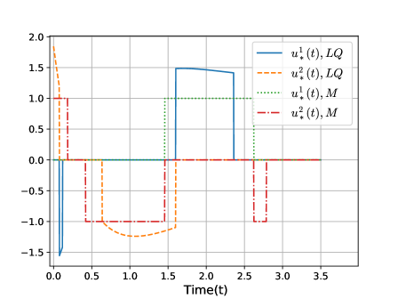
Figure 1. Multiplexed controls for the LQ and the Mayer problems.

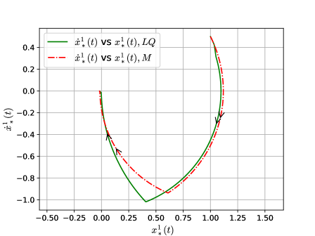
Figure 2. Phase portraits for the LQ and the Mayer problems.

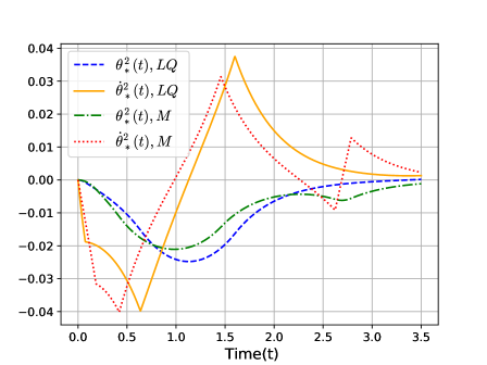
Figure 3. $\theta_{*}(\cdot),\dot{\theta}_{*}(\cdot)$, for the LQ and the Mayer problems.

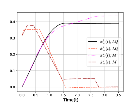
Figure 4. $x_{*}(\cdot),\dot{x}_{*}(\cdot)$ for the LQ and the Mayer problems.

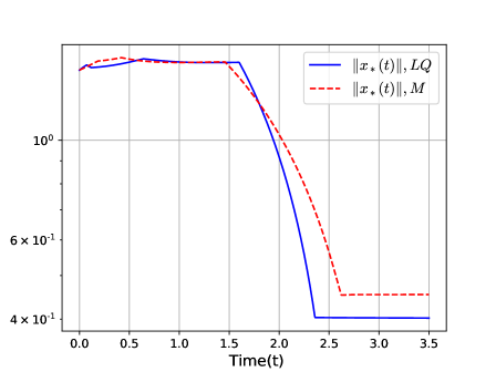
Figure 5. Norms of the states vs time for the LQ and the Mayer problems.

Appendix A A nonsmooth Pontryagin maximum principle

We need the following adaptation of [3, Theorem 22.26]:

Theorem A.1.

Let $\hat{t}\in\>]0,+\infty[$ and let $\mathbb{U}\subset\mathbb{R}^{m}$ be a non-empty Borel measurable set. Let a lower semicontinuous instantaneous cost function $\mathbb{R}^{d}\times\mathbb{U}\ni(\xi,\mu)\longmapsto\Lambda(\xi,\mu)\in\mathbb{R}$, with $\Lambda$ continuously differentiable in $\xi$ for every fixed $\mu$, and a continuously differentiable terminal cost function $\ell:\mathbb{R}^{d}\times\mathbb{R}^{d}\longrightarrow\mathbb{R}$ be given. Consider the optimal control problem

(A.1) $$\operatorname*{minimize}_{u} \quad\ell\bigl{(}x(0),x(\hat{t})\bigr{)}+\int_{0}^{\hat{t}}\Lambda\bigl{(}x(t),u(t)\bigr{)}\,\mathrm{d}t$$

$$\operatorname*{subject\ to} \quad\begin{cases}\dot{x}(t)=f\bigl{(}x(t),u(t)\bigr{)}\quad\text{for a.e.\ }t\in[0,\hat{t}],\\ u(t)\in\mathbb{U}\quad\text{for a.e.\ }t\in[0,\hat{t}],\\ u\text{ Lebesgue measurable},\\ \bigl{(}x(0),x(\hat{t})\bigr{)}\in E\subset\mathbb{R}^{d}\times\mathbb{R}^{d},\end{cases}$$

where $f:\mathbb{R}^{d}\times\mathbb{R}^{m}\longrightarrow\mathbb{R}^{d}$ is continuously differentiable, and $E$ is a closed set. For a real number $\eta$, we define the Hamiltonian $H^{\eta}$ by

$$H^{\eta}(p,x,u)\coloneqq\left\langle{p},{f(x,u)}\right\rangle-\eta\Lambda(x,u),\quad(p,x,u)\in\mathbb{R}^{d}\times\mathbb{R}^{d}\times\mathbb{U}.$$

If $[0,\hat{t}]\ni t\longmapsto\bigl{(}x_{\ast}(t),u_{\ast}(t)\bigr{)}\in\mathbb{R}^{d}\times\mathbb{U}$ is a local minimizer of (A.1), then there exist an absolutely continuous map $p:[0,\hat{t}]\longrightarrow\mathbb{R}^{d}$ and a scalar $\eta$ equal to $0$ or $1$, satisfying the nontriviality condition

(A.2) $$\bigl{(}\eta,p(t)\bigr{)}\neq 0\quad\text{for all }t\in[0,\hat{t}],$$

the transversality condition

(A.3) $$\bigl{(}p(0),-p(\hat{t})\bigr{)}\in\eta\nabla\ell\bigl{(}x_{\ast}(0),x_{\ast}(\hat{t})\bigr{)}+N_{E}^{L}\bigl{(}x_{\ast}(0),x_{\ast}(\hat{t})\bigr{)},$$

where $\nabla\ell$ is the gradient of $\ell$ and $N_{E}^{L}\bigl{(}x_{\ast}(0),x_{\ast}(\hat{t})\bigr{)}$ is the limiting normal cone to $E$ at the point $\bigl{(}x_{\ast}(0),x_{\ast}(\hat{t})\bigr{)}$, the adjoint equation

(A.4) $$-\dot{p}(t)=\partial_{x}H^{\eta}\bigl{(}p(t),\boldsymbol{\cdot},u_{\ast}(t)\bigr{)}(x_{\ast}(t))\quad\text{for a.e.\ }t\in[0,\hat{t}],$$

the Hamiltonian maximum condition

(A.5) $$H^{\eta}\bigl{(}p(t),x_{\ast}(t),u_{\ast}(t)\bigr{)}=\sup_{v\in\mathbb{U}}H^{\eta}\bigl{(}p(t),x_{\ast}(t),v\bigr{)}\quad\text{for a.e.\ }t\in[0,\hat{t}],$$

as well as the constancy of the Hamiltonian

(A.6) $$H^{\eta}\bigl{(}p(t),x_{\ast}(t),u_{\ast}(t)\bigr{)}=h\quad\text{for a.e.\ }t\in[0,\hat{t}]\text{ and some }h\in\mathbb{R}.$$

The quadruple $\bigl{(}\eta,p,x_{\ast},u_{\ast}\bigr{)}$ is known as the extremal lift of the optimal state-action trajectory $[0,\hat{t}]\ni t\longmapsto\bigl{(}x_{\ast}(t),u_{\ast}(t)\bigr{)}$. The number $\eta$ is called the abnormal multiplier. The abnormal case — when $\eta=0$ — may arise, e.g., when the constraints of the optimal control problem are so tight that the cost function plays no rôle in determining the solution. For instance, we have an abnormal case when the optimal solution $t\longmapsto\bigl{(}x_{\ast}(t),u_{\ast}(t)\bigr{)}$ is “isolated” in the sense that there is no other solution satisfying the end-point constraints in the vicinity — as measured by the supremum norm — of the optimal solution.

Theorem A.1 will yield characterizations of the controls that solve the optimal control problems (3.3) and (4.3); it constitutes the backbones of the proofs below.

Appendix B Multiplexed sparsest reachability: proofs

Recall that in §3 we defined $\lambda_{k}^{\prime}=\sum_{\ell\in\{1,\ldots,N\}\smallsetminus\{k\}}\lambda_{\ell}$ for each $k=1,\ldots,N$, and $\widetilde{\lambda}=\sum_{k=1}^{N}\lambda_{k}$.

Proof of Theorem 3.1 Notice first that Theorem A.1 applies directly to the optimal control problem (3.3). Indeed,

• $\mathbb{U}_{\mathrm{rch}}$ is a finite union of compact sets, and is therefore Borel measurable;

• the dynamics $f$ is given by the linear control system (2.3) and is therefore smooth;

• the instantaneous cost function $\Lambda(\xi,\mu)=-\sum_{k=1}^{N}\lambda_{k}\mathsf{1}_{\{0\}}(\mu^{k})$ is independent of the space variable $\xi$ and is lower semicontinuous in $\mu$;

• the terminal cost $\ell$ is identically $0$; and

• the boundary constraint set $E=\{(\bar{x},\hat{x})\}$ is a singleton, and is therefore closed.

Let the state-action trajectory $[0,\hat{t}]\ni t\longmapsto\bigl{(}x_{\ast}(t),u_{\ast}(t)\bigr{)}$ be a local minimizer of (3.3). For a real number $\eta$ we define the Hamiltonian

(B.1) $$(\mathbb{R}^{d_{1}}\times\cdots\times\mathbb{R}^{d_{N}})\times(\mathbb{R}^{d_{1}}\times\cdots\times\mathbb{R}^{d_{N}})\times\mathbb{U}_{\mathrm{rch}}$$

$$\quad\ni\left(\begin{pmatrix}p^{1}\\ \smash[t]{\vdots}\\ p^{N}\end{pmatrix},\begin{pmatrix}\xi^{1}\\ \smash[t]{\vdots}\\ \xi^{N}\end{pmatrix},\begin{pmatrix}\mu^{1}\\ \smash[t]{\vdots}\\ \mu^{N}\end{pmatrix}\right)\eqqcolon(p,\xi,\mu)\longmapsto$$

$$\quad H^{\eta}(p,\xi,\mu)\coloneqq\left\langle{p},{A\xi+B\mu}\right\rangle+\eta\sum_{k=1}^{N}\lambda_{k}\mathsf{1}_{\{0\}}(\mu^{k})$$

$$=\sum_{k=1}^{N}\left(\left\langle{p^{k}},{A_{k}\xi^{k}+B_{k}\mu^{k}}\right\rangle+\eta\lambda_{k}\mathsf{1}_{\{0\}}(\mu^{k})\right)\in\mathbb{R},$$

where we have employed the block-diagonal structure of $A$ and $B$ to arrive at the last equality.

By Theorem A.1, there exists an absolutely continuous map $[0,\hat{t}]\ni t\longmapsto p(t)\in\mathbb{R}^{d}$ (called an adjoint trajectory,) that, in view of the adjoint equation (A.4), solves

$$-\dot{p}(t)=\partial_{\xi}H^{\eta}\bigl{(}p(t),\cdot,u_{\ast}(t)\bigr{)}\bigl{(}x_{\ast}(t)\bigr{)}=A^{\top}p(t)\quad\text{for a.e.\ }t\in[0,\hat{t}],$$

or, in terms of the individual $N$ maps $(p^{k})_{k=1}^{N}$ obtained by projecting $p$ at each time to appropriate factors in an obvious way,

$$-\dot{p}^{k}(t)=A_{k}^{\top}p^{k}(t)\quad\text{for a.e.\ }t\in[0,\hat{t}],\quad k=1,\ldots,N.$$

Note that linearity of the right-hand sides ensure that there is a unique adjoint trajectory. The boundary conditions for the adjoint $p$ are obtained from the transversality conditions (A.3), and in our problem they turn out to be

$$\bigl{(}p(0),-p(\hat{t})\bigr{)}\in\mathbb{R}^{d}\times\mathbb{R}^{d},$$

in other words, the boundary conditions of $p$ are free.

The optimal control actions as functions of time are such that they satisfy the Hamiltonian maximum condition (A.5). For our problem this condition is: for a.e. $t\in[0,\hat{t}]$,

$$u_{\ast}(t)\in\operatorname*{arg\,max}_{\mu\in\mathbb{U}_{\mathrm{rch}}}H^{\eta}\bigl{(}p(t),x_{\ast}(t),\mu\bigr{)}$$

$$\quad=\operatorname*{arg\,max}_{\mu\in\mathbb{U}_{\mathrm{rch}}}\Biggl{\{}\sum_{k=1}^{N}\left(\left\langle{p^{k}(t)},{A_{k}x^{k}_{\ast}(t)+B_{k}\mu^{k}}\right\rangle+\eta\lambda_{k}\mathsf{1}_{\{0\}}(\mu^{k})\right)\Biggr{\}}$$

$$\quad=\operatorname*{arg\,max}_{\mu\in\mathbb{U}_{\mathrm{rch}}}\Biggl{\{}\sum_{k=1}^{N}\left(\left\langle{B_{k}^{\top}p^{k}(t)},{\mu^{k}}\right\rangle+\eta\lambda_{k}\mathsf{1}_{\{0\}}(\mu^{k})\right)\Biggr{\}}.$$

Denoting by $S\subset[0,\hat{t}]$ the full-measure set on which the preceding membership of $u_{\ast}$ holds, we fix $t\in S$. For this $t$, any arguemnt $\mu\coloneqq(\mu^{k})_{k=1}^{N}\in\mathbb{U}_{\mathrm{rch}}$ of the map

$$\mathbb{U}_{\mathrm{rch}}\ni\begin{pmatrix}\mu^{1}\\ \smash[t]{\vdots}\\ \mu^{N}\end{pmatrix}\longmapsto\sum_{k=1}^{N}\biggl{(}\left\langle{B_{k}^{\top}p{k}(t)},{\mu^{k}}\right\rangle+\eta\lambda_{k}\mathsf{1}_{\{0\}}(\mu^{k})\biggr{)}\in\mathbb{R}$$

has at most one non-zero $\mu^{k}$ due to the “star-shaped” structure of the set $\mathbb{U}_{\mathrm{rch}}$ defined in (3.1). For each $k=1,\ldots,N$, we let

$$\mathbb{U}^{(k)}\ni v\longmapsto\phi^{\eta}_{k}(t,v)\coloneqq\left\langle{B_{k}^{\top}p^{k}(t)},{v}\right\rangle\\ +\eta\bigl{(}\lambda_{k}\mathsf{1}_{\{0\}}(v)+\lambda_{k}^{\prime}\bigr{)}\in\mathbb{R},$$

and note that $\phi^{\eta}_{k}(t,\cdot)$ is upper semicontinuous; since the set $\mathbb{U}^{(k)}$ is compact by assumption,

$$\overline{\phi}^{\eta}_{k}(t)\coloneqq\sup_{v\in\mathbb{U}^{(k)}}\phi^{\eta}_{k}(t,v)$$

is attained on $\mathbb{U}^{(k)}$ by Weierstrass’s theorem [3, Exercise 2.14]. We let $\Phi^{\eta}(t,k)$ denote the non-empty set of maximizers of $\phi^{\eta}_{k}(t,\cdot)$, $k=1,\ldots,N$; i.e.,

(B.2) $$\Phi^{\eta}(t,k)\coloneqq\operatorname*{arg\,max}_{v\in\mathbb{U}^{(k)}}\phi^{\eta}_{k}(t,v),\quad k=1,\ldots,N.$$

Informally, at the time $t$ fixed above, we get the finite sequence $\bigl{(}\overline{\phi}^{\eta}_{k}(t)\bigr{)}_{k=1}^{N}$ of real numbers, and this finite sequence has a maximum element, say $\overline{\phi}^{\eta}_{k_{\ast}}(t)$; the optimal control action $u_{\ast}(t)=\bigl{(}u^{k}_{\ast}(t)\bigr{)}_{k=1}^{N}$ must be such that $u^{k_{\ast}}_{\ast}(t)\in\Phi^{\eta}(t,k_{\ast})$ and $u^{\ell}_{\ast}(t)=0$ for all $\ell\in\{1,\ldots,N\}\smallsetminus\{k_{\ast}\}$. By letting $t$ range over $S$, we have a characterization of $u_{\ast}$ on $S$. The behaviour of $u_{\ast}$ on $[0,\hat{t}]\smallsetminus S$ can, of course, be arbitrary. Formally, defining

(B.3) $$\Sigma^{\mathrm{rch}}_{\eta}(t)\coloneqq\begin{dcases*}\operatorname*{arg\,max}_{k\in\{1,\ldots,N\}}\overline{\phi}^{\eta}_{k}(t)&for $t\in S$,\\ \{1,\ldots,N\}&for $t\in[0,\hat{t}]\smallsetminus S$,\end{dcases*}$$

we arrive at a family of non-empty subsets of $\{1,\ldots,N\}$ parametrized by $t\in[0,\hat{t}]$; in other words, $\Sigma^{\mathrm{rch}}_{\eta}$ is a set-valued map from $[0,\hat{t}]$ into the power set of $\{1,\ldots,N\}$. Given $\Sigma^{\mathrm{rch}}_{\eta}$, any map (commonly known as a selector of the set-valued map $\Sigma^{\mathrm{rch}}_{\eta}$,)

$$[0,\hat{t}]\ni t\longmapsto\sigma^{\mathrm{rch}}_{\eta}(t)\in\Sigma^{\mathrm{rch}}_{\eta}(t)$$

gives us an admissible multiplexer. (Note that the Axiom of Choice [6, p. 8], guarantees that there always exists such a selector, and therefore, a multiplexer.) It follows that the set $(u^{k}_{\ast})_{k=1}^{N}$ of optimal controls constituting $u_{\ast}$ satisfies

(B.4) $$u^{k}_{\ast}(t)\in\begin{cases}\Phi^{\eta}\bigl{(}t,\sigma^{\mathrm{rch}}_{\eta}(t)\bigr{)}&\text{if }k=\sigma^{\mathrm{rch}}_{\eta}(t),\\ \{0\}&\text{otherwise},\end{cases}\quad k=1,\ldots,N,$$

$$\text{for all }t\in[0,\hat{t}].$$

It is time to provide more precise descriptions of the sets $\Phi^{\eta}(t,k)$ defined in (B.2). As asserted by Theorem A.1, only the two cases of $\eta=0$ or $\eta=1$ arise. If $\eta=0$, then for each $t\in S$

$$\Phi^{0}(t,k)=\operatorname*{arg\,max}_{v\in\mathbb{U}^{(k)}}\left\langle{B_{k}^{\top}p^{k}(t)},{v}\right\rangle\quad\text{for }k=1,\ldots,N,$$

and

$$\sigma^{\mathrm{rch}}(t)\in\operatorname*{arg\,max}_{k\in\{1,\ldots,N\}}\max_{v\in\mathbb{U}^{(k)}}\left\langle{B_{k}^{\top}p^{k}(t)},{v}\right\rangle.$$

If $\eta=1$, then for each $t\in S$

$$\Phi^{1}(t,k)=\operatorname*{arg\,max}_{v\in\mathbb{U}^{(k)}}\left\{\left\langle{B_{k}^{\top}p^{k}(t)},{v}\right\rangle+\lambda_{k}\mathsf{1}_{\{0\}}(v)\right\}$$

$$=\begin{dcases}\operatorname*{arg\,max}_{v\in\mathbb{U}^{(k)}}\left\langle{B_{k}^{\top}p^{k}(t)},{v}\right\rangle&\text{if }\max_{v\in\mathbb{U}^{(k)}}\left\langle{B_{k}^{\top}p^{k}(t)},{v}\right\rangle>\lambda_{k},\\ \{0\}\cup\operatorname*{arg\,max}_{v\in\mathbb{U}^{(k)}}\left\langle{B_{k}^{\top}p^{k}(t)},{v}\right\rangle&\text{if }\max_{v\in\mathbb{U}^{(k)}}\left\langle{B_{k}^{\top}p^{k}(t)},{v}\right\rangle=\lambda_{k},\\ \{0\}&\text{otherwise}.\end{dcases}$$

$$\quad\text{for }k=1,\ldots,N,$$

and

$$\sigma^{\mathrm{rch}}(t)\in\operatorname*{arg\,max}_{k\in\{1,\ldots,N\}}\max_{v\in\mathbb{U}^{(k)}}\Bigl{\{}\left\langle{B_{k}^{\top}p^{k}(t)},{v}\right\rangle+\lambda_{k}\mathsf{1}_{\{0\}}(v)+\lambda_{k}^{\prime}\Bigr{\}}.$$

Note that $\lambda_{k}^{\prime}$ is a constant in the definition of $\phi^{1}_{k}$, and plays no rôle in the determination of the set $\Phi^{1}(t,k)$. The value of $\overline{\phi}^{1}_{k}(t)$ at each $t\in S$, however, depends on this constant, and therefore, so does the set-valued map $t\longmapsto\Sigma^{\mathrm{rch}}_{1}(t)$ defined in (B.3), and therefore, also the map $t\longmapsto\sigma^{\mathrm{rch}}_{1}(t)$. Moreover, since $u_{\ast}$ is measurable, so is $\sigma^{\mathrm{rch}}$.

The constancy of the Hamiltonian (A.6) gives the final assertion of the theorem, thereby completing the proof. $\square$

Proof of Corollary 3.5 We retain the notations introduced in the proof of Theorem 3.1 above, and note that the only details that need to be supplied here are the sets $\Phi^{0}(t,k)$ and $\Phi^{1}(t,k)$ for each $t\in S$ and $k=1,\ldots,N$, corresponding to $\eta=0$ and $\eta=1$, respectively. To that end, note that if $\eta=0$, then

$$\Phi^{0}(t,k) =\operatorname*{arg\,max}_{v\in[-1,1]}\phi^{0}_{k}(t,v)=\operatorname*{arg\,max}_{v\in[-1,1]}B_{k}^{\top}p^{k}(t)v$$

$$=\operatorname{sgn}\big{(}B_{k}^{\top}p^{k}(t)\bigr{)},$$

where the set-valued map $\operatorname{sgn}$ defined in (1.1). If $\eta=1$, then

$$\Phi^{1}(t,k) =\operatorname*{arg\,max}_{v\in[-1,1]}\phi^{1}_{k}(t,v)$$

$$=\operatorname*{arg\,max}_{v\in[-1,1]}\Bigl{\{}B_{k}^{\top}p^{k}(t)v+\lambda_{k}\mathsf{1}_{\{0\}}(v)+\lambda_{k}^{\prime}\Bigr{\}}$$

$$=\begin{dcases}\operatorname{sgn}\bigl{(}B_{k}^{\top}p^{k}(t)\bigr{)}&\text{if }\left\lvert{B_{k}^{\top}p^{k}(t)}\right\rvert>\lambda_{k},\\ \{0\}\cup\operatorname{sgn}\bigl{(}B_{k}^{\top}p^{k}(t)\bigr{)}&\text{if }\left\lvert{B_{k}^{\top}p^{k}(t)}\right\rvert=\lambda_{k},\\ \{0\}&\text{otherwise}.\end{dcases}$$

The assertion follows at once. $\square$

Appendix C Multiplexed sparse LQ control: proof

Recall that in §4 we defined $\lambda_{k}^{\prime}=\sum_{\ell\in\{1,\ldots,N\}\smallsetminus\{k\}}\lambda_{\ell}$ for each $k=1,\ldots,N$, and $\widetilde{\lambda}=\sum_{k=1}^{N}\lambda_{k}$.

Proof of Theorem 4.1 Notice first that Theorem A.1 applies directly to the optimal control problem (4.3); the details being similar those elaborated in the Proof of Theorem 3.1 in §B, we omit them in the interest of brevity. Let the state-action trajectory $[0,\hat{t}]\ni t\longmapsto\bigl{(}x_{\ast}(t),u_{\ast}(t)\bigr{)}$ be a local minimizer of (3.3). For a real number $\eta$ we define the Hamiltonian

(C.1) $$(\mathbb{R}^{d_{1}}\times\cdots\times\mathbb{R}^{d_{N}})\times(\mathbb{R}^{d_{1}}\times\cdots\times\mathbb{R}^{d_{N}})\times\mathbb{U}_{\mathrm{LQ}}$$

$$\quad\ni\left(\begin{pmatrix}p^{1}\\ \smash[t]{\vdots}\\ p^{N}\end{pmatrix},\begin{pmatrix}\xi^{1}\\ \smash[t]{\vdots}\\ \xi^{N}\end{pmatrix},\begin{pmatrix}\mu^{1}\\ \smash[t]{\vdots}\\ \mu^{N}\end{pmatrix}\right)\eqqcolon(p,\xi,\mu)\longmapsto$$

$$\quad H^{\eta}(p,\xi,\mu)\coloneqq\left\langle{p},{A\xi+B\mu}\right\rangle$$

$$\quad-\eta\biggl{(}\tfrac{1}{2}\Bigl{(}\left\langle{\xi},{Q\xi}\right\rangle+\left\langle{\mu},{R\mu}\right\rangle\Bigr{)}-\sum_{k=1}^{N}\lambda_{k}\mathsf{1}_{\{0\}}(\mu^{k})\biggr{)}$$

$$=\sum_{k=1}^{N}\biggl{(}\left\langle{p^{k}},{A_{k}\xi^{k}+B_{k}\mu^{k}}\right\rangle$$

$$\qquad-\eta\Bigl{(}\tfrac{1}{2}\Bigl{(}\left\langle{\xi^{k}},{Q_{k}\xi^{k}}\right\rangle+\left\langle{\mu^{k}},{R_{k}\mu^{k}}\right\rangle\Bigr{)}-\lambda_{k}\mathsf{1}_{\{0\}}(\mu^{k})\Bigr{)}\biggr{)}\in\mathbb{R},$$

where we have employed the block-diagonal structure of $A$ and $B$ to arrive at the last equality.

By Theorem A.1, there exists an absolutely continuous map $[0,\hat{t}]\ni t\longmapsto p(t)\in\mathbb{R}^{d}$ (called the adjoint trajectory,) that, in view of the adjoint equation (A.4), solves

(C.2) $$\begin{aligned} -\dot{p}(t)&=\partial_{\xi}H^{\eta}\bigl{(}p(t),\cdot,u_{\ast}(t)\bigr{)}\bigl{(}x_{\ast}(t)\bigr{)}\\ &=A^{\top}p(t)+\eta Qx_{\ast}(t)\end{aligned}\quad\text{for a.e.\ }t\in[0,\hat{t}],$$

or, in terms of the individual $N$ maps $(p^{k})_{k=1}^{N}$ obtained by projecting $p$ at each time to appropriate factors in an obvious way,

$$-\dot{p}^{k}(t)=A_{k}^{\top}p^{k}(t)+\eta Q_{k}x^{k}_{\ast}(t)\quad\text{for a.e.\ }t\in[0,\hat{t}],\quad k=1,\ldots,N.$$

Linearity of the right-hand sides ensure that there is a unique adjoint trajectory. The boundary conditions for the adjoint $p$ are obtained from the transversality conditions (A.3), and in our problem they turn out to be

$$\bigl{(}p(0),-p(\hat{t})\bigr{)}\in\mathbb{R}^{d}\times\{\eta\hat{Q}x_{\ast}(\hat{t})\};$$

in other words, the initial condition of $p$ is free, and the final condition is $p(\hat{t})=-\eta\hat{Q}x_{\ast}(\hat{t})$.

Theorem A.1 admits only two cases of $\eta$ — $0$ or $1$. We claim that the case of $\eta=0$ does not arise in (4.3). Indeed, if $\eta=0$, then the final boundary condition of each $p^{k}$ is $0$, leading to $p(\hat{t})=0$, and the forcing term on the right-hand side of (C.2) also vanishes. In view of the resulting linearity of (C.2) with final condition equal to $0$, the entire trajectory $p$ vanishes. This contradicts the non-triviality condition (A.2) of Theorem A.1. Therefore, $\eta$ must be equal to $1$, to which we commit and henceforth write $H$ instead of $H^{1}$.

The optimal control actions as functions of time are such that they satisfy the Hamiltonian maximum condition (A.5). For our problem this condition is: for a.e. $t\in[0,\hat{t}]$,

$$u_{\ast}(t)\in\operatorname*{arg\,max}_{\mu\in\mathbb{U}_{\mathrm{LQ}}}H\bigl{(}p(t),x_{\ast}(t),\mu\bigr{)}$$

$$\quad=\operatorname*{arg\,max}_{\mu\in\mathbb{U}_{\mathrm{LQ}}}\Biggl{\{}\sum_{k=1}^{N}\biggl{(}\left\langle{p^{k}(t)},{A_{k}x^{k}_{\ast}(t)+B_{k}\mu^{k}}\right\rangle$$

$$\qquad\qquad\qquad-\Bigl{(}\tfrac{1}{2}\left\langle{\xi^{k}},{Q_{k}\xi^{k}}\right\rangle+\tfrac{1}{2}\left\langle{\mu^{k}},{R_{k}\mu^{k}}\right\rangle-\lambda_{k}\mathsf{1}_{\{0\}}(\mu^{k})\Bigr{)}\biggr{)}\Biggl{\}}$$

$$\quad=\operatorname*{arg\,max}_{\mu\in\mathbb{U}_{\mathrm{LQ}}}\Biggl{\{}\sum_{k=1}^{N}\biggl{(}\left\langle{B_{k}^{\top}p^{k}(t)},{\mu^{k}}\right\rangle-\tfrac{1}{2}\left\langle{\mu^{k}},{R_{k}\mu^{k}}\right\rangle+\lambda_{k}\mathsf{1}_{\{0\}}(\mu^{k})\biggr{)}\Biggr{\}}.$$

Denoting by $S\subset[0,\hat{t}]$ the full-measure set on which the preceding membership of $u_{\ast}$ holds, we fix $t\in S$. For this $t$, any argument $\mu\coloneqq(\mu^{k})_{k=1}^{N}\in\mathbb{U}_{\mathrm{LQ}}$ of the map

$$\mathbb{U}_{\mathrm{LQ}}\ni\begin{pmatrix}\mu^{1}\\ \smash[t]{\vdots}\\ \mu^{N}\end{pmatrix}\longmapsto\sum_{k=1}^{N} \biggl{(}\left\langle{B_{k}^{\top}p^{k}(t)},{\mu^{k}}\right\rangle$$

$$-\tfrac{1}{2}\left\langle{\mu^{k}},{R_{k}\mu^{k}}\right\rangle+\lambda_{k}\mathsf{1}_{\{0\}}(\mu^{k})\biggr{)}\in\mathbb{R}$$

has at most one non-zero $\mu^{k}$ due to the star-shaped conical structure of the set $\mathbb{U}_{\mathrm{LQ}}$ defined in (4.2). For each $k=1,\ldots,N$, we let

$$\mathbb{R}^{m_{k}}\ni v\longmapsto\psi_{k}(t,v)\coloneqq\left\langle{B_{k}^{\top}p^{k}(t)},{v}\right\rangle-\tfrac{1}{2}\left\langle{v},{R_{k}v}\right\rangle\\ +\lambda_{k}\mathsf{1}_{\{0\}}(v)+\lambda_{k}^{\prime}\in\mathbb{R}.$$

Note that the first two terms comprising $\psi_{k}(t,\cdot)$ define a strictly concave function due to positive definiteness of the matrix $R_{k}$, and the second two terms are bounded above. Moreover, $\psi_{k}(t,\cdot)$ is upper semicontinuous, and satisfies $\psi_{k}(t,v)\xrightarrow[\left\lVert{v}\right\rVert\to+\infty]{}-\infty$; therefore,

(C.3) $$\overline{\psi}_{k}(t)\coloneqq\sup_{v\in\mathbb{R}^{m_{k}}}\psi_{k}(t,v)$$

is attained on $\mathbb{R}^{m_{k}}$ by standard arguments that ultimately rely on Weierstrass’s theorem [3, Exercise 2.14]. We let $\Psi(t,k)$ denote the non-empty set of maximizers of $\psi_{k}(t,\cdot)$, $k=1,\ldots,N$; i.e.,

(C.4) $$\Psi(t,k)\coloneqq\operatorname*{arg\,max}_{v\in\mathbb{R}^{m_{k}}}\psi_{k}(t,v),\quad k=1,\ldots,N.$$

As we shall see momentarily, more than one maximizers of each $\psi_{k}(t,\cdot)$ may exist. Informally, at the time $t$ fixed above, we get the finite sequence $\bigl{(}\overline{\psi}_{k}(t)\bigr{)}_{k=1}^{N}$ of real numbers, and this finite sequence has a maximum element, say $\overline{\psi}_{k_{\ast}}(t)$; the optimal control action $u_{\ast}(t)=\bigl{(}u^{k}_{\ast}(t)\bigr{)}_{k=1}^{N}$ must be such that $u^{k_{\ast}}_{\ast}(t)\in\Psi(t,k_{\ast})$ and $u^{\ell}_{\ast}(t)=0$ for all $\ell\in\{1,\ldots,N\}\smallsetminus\{k_{\ast}\}$. By letting $t$ range over $S$, we have a characterization of $u_{\ast}$ on $S$. The behaviour of $u_{\ast}$ on $[0,\hat{t}]\smallsetminus S$ can, of course, be arbitrary. Formally, defining

(C.5) $$\Sigma^{\mathrm{LQ}}(t)\coloneqq\begin{dcases}\operatorname*{arg\,max}_{k\in\{1,\ldots,N\}}\overline{\psi}_{k}(t)&\text{for }t\in S,\\ \{1,\ldots,N\}&\text{for }t\in[0,\hat{t}]\smallsetminus S,\end{dcases}$$

we arrive at a family of non-empty subsets of $\{1,\ldots,N\}$ parametrized by $t\in[0,\hat{t}]$; in other words, $\Sigma^{\mathrm{LQ}}$ is a set-valued map from $[0,\hat{t}]$ into the power set of $\{1,\ldots,N\}$. Given $\Sigma^{\mathrm{LQ}}$, any map (i.e., any selector of the set-valued map $\Sigma^{\mathrm{LQ}}$,)

$$[0,\hat{t}]\ni t\longmapsto\sigma^{\mathrm{LQ}}(t)\in\Sigma^{\mathrm{LQ}}(t)$$

gives us an admissible multiplexer. (The Axiom of Choice [6, p. 8] guarantees the existence of such a selector, and therefore, a multiplexer.) It follows that the set $(u^{k}_{\ast})_{k=1}^{N}$ of optimal controls constituting $u_{\ast}$ satisfies

(C.6) $$u^{k}_{\ast}(t)\in\begin{cases}\Psi\bigl{(}t,\sigma^{\mathrm{LQ}}(t)\bigr{)}&\text{if }k=\sigma^{\mathrm{LQ}}(t),\\ \{0\}&\text{otherwise},\end{cases}\quad k=1,\ldots,N,$$

$$\text{for all }t\in[0,\hat{t}].$$

We provide more precise descriptions of the sets $\Psi(t,k)$ defined in (C.4): For each $t\in S$ and $k=1,\ldots,N$,

$$\Psi(t,k) =\operatorname*{arg\,max}_{v\in\mathbb{R}^{m_{k}}}\left\{\left\langle{B_{k}^{\top}p^{k}(t)},{v}\right\rangle-\tfrac{1}{2}\left\langle{v},{R_{k}v}\right\rangle+\lambda_{k}\mathsf{1}_{\{0\}}(v)\right\}$$

$$=\begin{cases}\bigl{\{}R_{k}^{-1}B_{k}^{\top}p^{k}(t)\bigr{\}}&\text{if }\left\lVert{p^{k}(t)}\right\rVert_{B_{k}R_{k}^{-1}B_{k}^{\top}}^{2}>2\lambda_{k},\\ \{0\}\cup\bigl{\{}R_{k}^{-1}B_{k}^{\top}p^{k}(t)\bigr{\}}&\text{if }\left\lVert{p^{k}(t)}\right\rVert_{B_{k}R_{k}^{-1}B_{k}^{\top}}^{2}=2\lambda_{k},\\ \{0\}&\text{otherwise},\end{cases}$$

Note that $\lambda_{k}^{\prime}$ is a constant in the definition of $\psi_{k}$, and plays no rôle in the determination of the set $\Psi(t,k)$. It does, however, influence the value of $\overline{\psi}_{k}(t)$ at each $t\in S$, and therefore, also the set-valued map $t\longmapsto\Sigma^{\mathrm{LQ}}(t)$ defined in (C.5).

The numbers $\bigl{(}\overline{\psi}_{k}(t)\bigr{)}_{k=1}^{N}$ defined in (C.3) admit the following concrete description:

$$\overline{\psi}_{k}(t) =\begin{cases}\lambda_{k}^{\prime}+\frac{1}{2}\left\lVert{p^{k}(t)}\right\rVert_{B_{k}R_{k}^{-1}B_{k}^{\top}}^{2}&\text{if }\left\lVert{p^{k}(t)}\right\rVert_{B_{k}R_{k}^{-1}B_{k}^{\top}}^{2}\geqslant 2\lambda_{k},\\ \widetilde{\lambda}&\text{otherwise},\end{cases}$$

$$\text{for all }t\in S.$$

Finally, for each $t\in S$,

$$\sigma^{\mathrm{LQ}}(t)\in$$

$$\operatorname*{arg\,max}_{k\in\{1,\ldots,N\}}\begin{cases}\lambda_{k}^{\prime}+\frac{1}{2}\left\lVert{p^{k}(t)}\right\rVert_{B_{k}R_{k}^{-1}B_{k}^{\top}}^{2}&\text{if }\left\lVert{p^{k}(t)}\right\rVert_{B_{k}R_{k}^{-1}B_{k}^{\top}}^{2}\geqslant 2\lambda_{k},\\ \widetilde{\lambda}&\text{otherwise}.\end{cases}$$

Measurability of $\sigma^{\mathrm{LQ}}$ follows from the assumption that $u_{\ast}$ is measurable. The steps above immediately lead to the assertion. $\square$

Appendix D Multiplexed sparse Mayer problem: proof

Recall that in §5 we defined $\lambda_{k}^{\prime}=\sum_{\ell\in\{1,\ldots,N\}\smallsetminus\{k\}}\lambda_{\ell}$ for each $k=1,\ldots,N$, and $\widetilde{\lambda}=\sum_{k=1}^{N}\lambda_{k}$. Proof of Theorem 5.2 Theorem A.1 applies to (5.2) because

• $\mathbb{U}_{\mathrm{M}}$ is a finite union of compact sets, and is therefore Borel measurable;

• the dynamics $f$ is given by the linear control system (2.3) and is therefore smooth;

• the instantaneous cost function $\Lambda(\xi,\mu)=-\sum_{k=1}^{N}\lambda_{k}\mathsf{1}_{\{0\}}(\mu^{k})$ is independent of the space variable $\xi$ and is lower semicontinuous in $\mu$;

• the terminal cost $\ell(\bar{\xi},\hat{\xi})=\frac{1}{2}\left\langle{\hat{\xi}-\hat{x}},{\hat{Q}\bigl{(}\hat{\xi}-\hat{x}\bigr{)}}\right\rangle$ is smooth; and

• the boundary constraint set $E=\{\bar{x}\}\times\mathbb{R}^{d}$ is closed.

Let the state-action trajectory $[0,\hat{t}]\ni t\longmapsto\bigl{(}x_{\ast}(t),u_{\ast}(t)\bigr{)}$ be a local minimizer of (5.2). For $\eta\in\mathbb{R}$ we define the Hamiltonian

(D.1) $$(\mathbb{R}^{d_{1}}\times\cdots\times\mathbb{R}^{d_{N}})\times(\mathbb{R}^{d_{1}}\times\cdots\times\mathbb{R}^{d_{N}})\times\mathbb{U}_{\mathrm{M}}$$

$$\quad\ni\left(\begin{pmatrix}p^{1}\\ \smash[t]{\vdots}\\ p^{N}\end{pmatrix},\begin{pmatrix}\xi^{1}\\ \smash[t]{\vdots}\\ \xi^{N}\end{pmatrix},\begin{pmatrix}\mu^{1}\\ \smash[t]{\vdots}\\ \mu^{N}\end{pmatrix}\right)\eqqcolon(p,\xi,\mu)\longmapsto$$

$$\quad H^{\eta}(p,\xi,\mu)\coloneqq\left\langle{p},{A\xi+B\mu}\right\rangle+\eta\sum_{k=1}^{N}\lambda_{k}\mathsf{1}_{\{0\}}(\mu^{k})$$

$$\quad=\sum_{k=1}^{N}\biggl{(}\left\langle{p^{k}},{A_{k}\xi^{k}+B_{k}\mu^{k}}\right\rangle+\eta\lambda_{k}\mathsf{1}_{\{0\}}(\mu^{k})\biggr{)}\in\mathbb{R},$$

By Theorem A.1 there exists an absolutely continuous map $[0,\hat{t}]\ni t\longmapsto p(t)\in\mathbb{R}^{d}$, the adjoint trajectory, that solves

$$-\dot{p}(t)=\partial_{\xi}H^{\eta}\bigl{(}p(t),\cdot,u_{\ast}(t)\bigr{)}\bigl{(}x_{\ast}(t)\bigr{)}=A^{\top}p(t)\quad\text{for a.e.\ }t\in[0,\hat{t}],$$

or equivalently,

(D.2) $$-\dot{p}^{k}(t)=A_{k}^{\top}p^{k}(t)\quad\text{for a.e.\ }t\in[0,\hat{t}],\quad k=1,\ldots,N.$$

The boundary conditions for the adjoint $p$ are obtained from the transversality conditions (A.3), and for our problem (D.2) they are given by

$$\bigl{(}p(0),-p(\hat{t})\bigr{)}\in\mathbb{R}^{d}\times\bigl{\{}\eta\hat{Q}\bigl{(}x_{\ast}(\hat{t})-\hat{x}\bigr{)}\bigr{\}}.$$

In other words, the differential equations for $(p^{k})_{k=1}^{N}$ have specific terminal boundary constraints and free initial conditions; therefore, they have to be solved in reverse time.

Theorem A.1 admits only two values of $\eta$. We claim that the case of $\eta=0$ does not arise in (5.2). Indeed, if $\eta=0$, then the final boundary condition of each $p^{k}$ is $0$, leading to $p(\hat{t})=0$; since the linear adjoint differential equations in (D.2) have no forcing terms, the entire trajectory of $p$ must vanish. This contradicts the non-triviality condition (A.2) of Theorem A.1. Therefore, $\eta=1$, and we write $H$ instead of $H^{1}$ henceforth.

The optimal control actions as functions of time must satisfy the Hamiltonian maximum condition (A.5): for a.e. $t\in[0,\hat{t}]$,

$$u_{\ast}(t) \in\operatorname*{arg\,max}_{\mu\in\mathbb{U}_{\mathrm{M}}}H\bigl{(}p(t),x_{\ast}(t),\mu\bigr{)}$$

$$=\operatorname*{arg\,max}_{\mu\in\mathbb{U}_{\mathrm{M}}}\biggl{\{}\sum_{k=1}^{N}\left\langle{B_{k}^{\top}p^{k}(t)},{\mu^{k}}\right\rangle+\lambda_{k}\mathsf{1}_{\{0\}}(\mu^{k})\biggr{\}}.$$

Proceeding as in the proof of Theorem 3.1 we see that

$$u^{k}_{\ast}(t)\in\begin{dcases}\operatorname*{arg\,max}_{v\in\mathbb{U}^{(k)}}\left\langle{B_{k}^{\top}p^{k}(t)},{v}\right\rangle&\text{if}\max_{v\in\mathbb{U}^{(k)}}\left\langle{B_{k}^{\top}p^{k}(t)},{v}\right\rangle>\lambda_{k},\\ \{0\}\cup\operatorname*{arg\,max}_{v\in\mathbb{U}^{(k)}}\left\langle{B_{k}^{\top}p^{k}(t)},{v}\right\rangle&\text{if}\max_{v\in\mathbb{U}^{(k)}}\left\langle{B_{k}^{\top}p^{k}(t)},{v}\right\rangle=\lambda_{k},\\ \{0\}&\text{otherwise}.\end{dcases}$$

$$\qquad\text{for }k=1,\ldots,N,$$

and

$$\sigma^{\mathrm{M}}(t)\in\operatorname*{arg\,max}_{k\in\{1,\ldots,N\}}\max_{v\in\mathbb{U}^{(k)}}\Bigl{\{}\left\langle{B_{k}^{\top}p^{k}(t)},{v}\right\rangle+\lambda_{k}\mathsf{1}_{\{0\}}(v)+\lambda_{k}^{\prime}\Bigr{\}}.$$

Since $u_{\ast}$ is measurable, so is $\sigma^{\mathrm{M}}$. The constancy of the Hamiltonian (A.6) gives the final assertion of the theorem, completing the proof. $\square$

References

- [1] M. S. Branicky, S. M. Phillips, and W. Zhang, Scheduling and feedback co-design for networked control systems, in Proceedings of the 41st IEEE Conference on Decision and Control, 2002., vol. 2, Dec 2002, pp. 1211–1217 vol.2.
- [2] D. Chatterjee, M. Nagahara, D. E. Quevedo, and K. S. M. Rao, Characterization of maximum hands-off control, Systems & Control Letters, 94 (2016), pp. 31–36.
- [3] F. H. Clarke, Functional Analysis, Calculus of Variations and Optimal Control, vol. 264 of Graduate Texts in Mathematics, Springer, London, 2013.
- [4] C. M. de Farias, L. Pirmez, F. C. Delicato, W. Li, A. Y. Zomaya, and J. N. de Souza, A scheduling algorithm for shared sensor and actuator networks, in The International Conference on Information Networking 2013 (ICOIN), Jan 2013, pp. 648–653.
- [5] A. V. der Maas, Y. F. Steinbuch, A. Boverhof, and W. P. M. H. Heemels, Switched control of a scara robot with shared actuation resources, IFAC-PapersOnLine, 50 (2017), pp. 1931 – 1936. 20th IFAC World Congress.
- [6] E. DiBenedetto, Real Analysis, Birkhäuser Advanced Texts, Birkhäuser, Boston, 2002.
- [7] M. Fardad, F. Lin, and M. R. Jovanović, Design of optimal sparse interconnection graphs for synchronization of oscillator networks, IEEE Transactions on Automatic Control, 59 (2014), pp. 2457–2462.
- [8] C. Farias, L. Pirmez, F. Delicato, L. Carmo, W. Li, A. Y. Zomaya, and J. N. de Souza, Multisensor data fusion in shared sensor and actuator networks, in 17th International Conference on Information Fusion (FUSION), July 2014, pp. 1–8.
- [9] A. F. Filippov, Differential Equations with Discontinuous Righthand Sides, vol. 18 of Mathematics and its Applications (Soviet Series), Kluwer Academic Publishers Group, Dordrecht, 1988. Translated from the Russian.
- [10] W. H. Fleming and R. W. Rishel, Deterministic and Stochastic Optimal Control, Applications of Mathematics 1, Springer, 1975.
- [11] M. Jovanović and F. Lin, Sparse quadratic regulator, in Proceedings of the European Control Conference (ECC), 2013, pp. 1047–1052.
- [12] D. Liberzon, Calculus of Variations and Optimal Control Theory, Princeton University Press, Princeton, NJ, 2012. A concise introduction.
- [13] M. Nagahara, D. E. Quevedo, and D. Nešić, Maximum hands-off control: a paradigm of control effort minimization, IEEE Transactions on Automatic Control, 61 (2016).
- [14] B. Polyak, M. Khlebnikov, and P. Shcherbakov, Sparse feedback in linear control systems, Automation and Remote Control, 75 (2014), pp. 2099–2111.
- [15] I. M. Ross, A Primer on Pontryagin’s Principle in Optimal Control, Collegiate Publishers, 2nd ed., 2015.
- [16] I. Saha, S. Baruah, and R. Majumdar, Dynamic scheduling for networked control systems, in Proceedings of the 18th International Conference on Hybrid Systems: Computation and Control, HSCC ’15, ACM, 2015, pp. 98–107.
- [17] S. Srikant and D. Chatterjee, A jammer’s perspective of reachability and LQ optimal control, Automatica, 70 (2016), pp. 295–302.
- [18] L. Zhang and D. Hristu-Varsakelis, Communication and control co-design for networked control systems, Automatica, 42 (2006), pp. 953 – 958.