Non-adiabatic mass correction to the rovibrational states of molecules. Numerical application for the H${}_{2}^{+}$ molecular ion

Abstract

General transformation expressions of the second-order non-adiabatic Hamiltonian of the atomic nuclei, including the kinetic-energy correction terms, are derived upon the change from laboratory-fixed Cartesian coordinates to general curvilinear coordinate systems commonly used in rovibrational computations. The kinetic-energy or so-called “mass-correction” tensor elements are computed with the stochastic variational method and floating explicitly correlated Gaussian functions for the H${}_{2}^{+}$ molecular ion in its ground electronic state. (Further numerical applications for the ⁴He${}_{2}^{+}$ molecular ion are presented in the forthcoming paper, Paper II.) The general, curvilinear non-adiabatic kinetic energy operator expressions are used in the examples and non-adiabatic rovibrational energies and corrections are determined by solving the rovibrational Schrödinger equation including the diagonal Born–Oppenheimer as well as the mass-tensor corrections.

I Introduction

The mass (or better: kinetic-energy) correction terms in the second-order non-adiabatic rovibrational Hamiltonian has been re-discovered in several very different contexts since the advent of quantum mechanics. In contrast to the diagonal Born–Oppenheimer (DBOC) correction, the mass-correction terms have been rarely included in rovibrational computations, apart from the common arguments of using atomic instead of nuclear masses. The practice of using atomic masses is confirmed by a posteriori by obtaining a better agreement with the experimentally observed rovibrational transitions (with or without accounting for any relativistic and radiative effects in the computations).

The earliest account of the kinetic-energy correction terms which we mention here is from 1964 by Fisk and Kirtman Fisk and Kirtman (1964) who wrote about a velocity-dependent effective potential energy surface (PES), which they obtained obtained using van Vleck’s perturbation theory approach. Bunker and Moss derived effective non-adiabatic rovibrational Hamiltonians using van Vleck’s perturbation theory for di- Bunker and Moss (1977) and triatomic Bunker and Moss (1980) molecules and used their formalism for diatomics Bunker et al. (1977). Later Schwenke elaborated on these correction terms and computed them in curvilinear coordinates for diatomic molecules Schwenke (2001a) as well as for the triatomic H₂O molecule Schwenke (2001b).

Pachucki and Komasa introduced non-adiabatic perturbation theory Pachucki and Komasa (2008) and arrived at the same mass-correction functions for diatomic molecules, which they successfully used for a series of systems Pachucki and Komasa (2009, 2012), including the H₂ molecule in its ground electronic state Pachucki and Komasa (2009). Kutzelnigg Kutzelnigg (2007) and Jaquet and Kutzelnigg Jaquet and Kutzelnigg (2008) derived and computed mass-correction functions by starting out from a careful consideration of the separation of the center of mass and the total mass of the molecule in an adiabatic theory. There were also more empirical proposals for the “rotational” and “vibrational” mass correction functions of di- and triatomic molecules, which connected the mass correction to the electron density assignable to the nuclei Diniz et al. (2013).

In an elegant and formal series of work, Teufel and co-workers introduced adiabatic perturbation theory in quantum dynamics and used it for the Born–Oppenheimer (BO) separation of the electronic and nuclear degrees of freedom, the coupling of which can be characterized by the square root of the electron-to-nucleus mass ratio. The authors identified the almost invariant subspace for the electronic problem and using this subspace they derived an effective Hamiltonian for the quantum mechanical motion of the atomic nuclei corresponding to an isolated electronic state (separated with gaps from all other electronic states). Expanding this effective Hamiltonian in terms of increasing orders of the coupling parameter, corrections are obtained to the (zeroth order) BO Hamiltonian of the atomic nuclei. The second-order Hamiltonian contains the DBOC and mass-correction tensor obtained also in other perturbative procedures. Teufel and co-workers mention the derivation of Weigert and Littlejohn from 1993 Weigert and Littlejohn (1993) using Weyl calculus for formally diagonalizing the multicomponent wave equation, an approach which resulted a similar effective Hamiltonian for the nuclear motion.

Most recently, independent of earlier work, the mass correction tensor Scherrer et al. (2017) was derived from exact factorization through nuclear velocity perturbation theory Scherrer et al. (2015), which successfully provides a theoretical framework also for vibrational circular dichroism.

The relation of the mass-correction tensor to the computation of magnetic properties has been observed (for diatomics) also by Bunker and Moss Bunker and Moss (1977). Herman and Asgharian Herman and Asgharian (1966) and Herman and Ogilvie Herman and Ogilvie (1998) pointed out its connection to the electronic contribution to the rotational and vibrational (paramagnetic) $g$-factors (see also Ref. Ogilvie (1998)). For example, the $g$-factors computed using a linear response method with full-CI/aug-cc-pVTZ by Sauer et al. Sauer et al. (2005) for HeH⁺ were found to be in a few % agreement with computations of Pachucki and Komasa Pachucki and Komasa (2012) using the optimized explicitly correlated Gaussian functions (ECGs). Ogilvie and co-workers Bak et al. (2005) (as well as Pachuchki and Komasa Pachucki and Komasa (2009)) computed the vibrational and rotational $g$-factors and adiabatic corrections for the hydrogen molecule. The vibrational $g$-factor was computed for the bending mode of HCN in Ref. Braun et al. (1996)

Obviously, there has been a substantial theoretical and computational progress over the past half a century concerning the theory and computational applications of the complete second-order rovibrational Hamiltonian, which includes the mass-correction tensor. We find it fascinating that the same quantity, i.e., the same mass-correction term, appear in a variety of contexts and essentially the same quantity has been obtained starting from various directions and by using very different (perturbational) formalisms. It would be interesting to explore the various aspects and theoretical connections between the different derivations.

After recognizing all these earlier, somewhat parallel developments, it is interesting to notice that the mass-correction tensor is not routinely included in the nowadays numerically “exact” rovibrational computations, in which however the PES (almost routinely) includes the diagonal Born–Oppenheimer correction, which is also a second-order term in the non-adiabatic Hamiltonian (see for example, Ref. Kutzelnigg (2007); Panati et al. (2007)). The accuracy of the present-day high-resolution (precision) spectroscopy measurements (see for example Ref. Semeria et al. (2016) discussed in Paper II Ma (1)) implies that one has to go beyond the empirical non-adiabatic corrections in which the nuclear masses are arbitrarily replaced with some effective (constant, usually the atomic) masses (which are thought to account for some of the mass-correction tensor effects). In particular, there are at least two important “families” of small effects to be accounted for in the computations: “non-adiabatic corrections” and “relativistic and radiative corrections”—both represent challenges for a rigorous theoretical description.

We wonder why the computation and the use of the mass-correction tensor did not become routine in rovibrational studies. We think and agree with the authors of Ref. Scherrer et al. (2017) that for a widespread applicability it would be important to compute the mass-correction tensor in Cartesian coordinates (Schwenke in Ref. Schwenke (2001b) also mentions this direction as possible further development for his curvilinear derivation). In particular, the widespread and general computation of the DBOC has become possible by its formulation and computation in simple Cartesian coordinates following Handy and co-workers Handy and Lee (1996); Ioannou et al. (1996); Handy et al. (1986) (instead of using the system- and coordinate-dependent form). The laboratory-frame Cartesian coordinate expression of the DBOC was later confirmed in a stringent numerical test by Cencek and Kutzelnigg Cencek and Kutzelnigg (1997) and was explained in formal terms by Kutzelnigg Kutzelnigg (1997). The DBOC is a scalar quantity, while the mass-correction factor is a tensor. As it was also discussed by Schwenke Schwenke (2001b), the mass-correction tensor is an inherently more complicated mathematical object. Nevertheless, it can be computed using Cartesian coordinates with a selected frame for the nuclei from the electronic energies and wave-functions as it was demonstrated in Ref. Scherrer et al. (2017) at the equilibrium structures of the H₂, H₂O, and CH₃OH molecules.

In what follows, we derive the rovibrational Hamiltonian including the mass-correction term starting from laboratory-frame Cartesian coordinates to a general curvilinear coordinate system, in the spirit of the numerical-kinetic energy operator approach used in the GENIUSH protocol Mátyus et al. (2009). For the electronic structure computations, (due to the lack of any widely available electronic structure method) we employ our in-house developed computer program, QUANTEN (QUANTum mechanical treatment of Electrons and atomic Nuclei), which uses the variational method and explicitly correlated Gaussian functions to solve the Schrödinger equation. If all charges belong to the quantum system we solve a pre-Born–Oppenheimer problem Mátyus and Reiher (2012); Mátyus (2013, 2018). For the present work, we extended QUANTEN for the case of fixed external charges to solve the electronic Schrödinger equation. In the second part of the paper, we explain how the necessary adiabatic and non-adiabatic quantities are computed.

Applications for a variety of poly-atomic and poly-electronic molecules will become possible when the Cartesian mass-correction tensor can be computed with an efficient electronic structure package over a broad range of molecular configurations. The implementation of the mass-correction tensor computed in Cartesian coordinates in a general curvilinear rovibrational program (e.g., the GENIUSH program) should be straightforward based on the expressions derived in the first part of the article. To demonstrate the applicability of the expressions and to show numerical examples we make the calculations explicit and give numerical results for the homonuclear diatomic H${}_{2}^{+}$ molecular ion and further applications follow for ⁴He${}_{2}^{+}$ in Paper II Ma (1).

II The second-order non-adiabatic Hamiltonian

In this section, we re-iterate the second-order non-adiabatic Hamiltonian derived by Panati, Spohn and Teufel Panati et al. (2007) and adjust some of the notation to that used in the derivation from exact factorization Scherrer et al. (2017). Both derivations have been carried out in laboratory-frame Cartesian coordinates, and these general, $N$-atomic expressions provide the most convenient starting point for our work. The second-order non-adiabatic Hamiltonian of the atomic nuclei corresponding to a single electronic state (in Hartree atomic units $\hbar=m_{\mathrm{e}}=a_{0}=1$) is:

$$\hat{H}^{\text{(2)}}=-\sum_{i=1}^{N}\sum_{a}\frac{1}{2m_{\text{n}}}\partial_{R_{ia}}^{2}+\sum_{i,j=1}^{N}\sum_{a,b}\frac{1}{2m_{\text{n}}}\partial_{R_{ia}}\left[\frac{1}{m_{\text{n}}}\mathcal{A}_{ia,jb}\right]\partial_{R_{jb}}+V+\sum_{i=1}^{N}\sum_{a}\frac{1}{m_{\text{n}}}U_{ia}$$ (1)

where $\partial_{R_{ia}}=\partial/\partial_{R_{ia}}$ is short notation for the partial derivative with respect to the laboratory-frame Cartesian coordinates, $R_{ia}$ ($a=X,Y,Z$). The first and thrid term is the BO kinetic energy operator and the potential energy surface (PES), respectively. The latter equals to the electronic energy, $E^{\text{(el)}}$, the eigenvalue of the electronic Schrödinger equation:

$$\hat{H}^{\text{(el)}}\psi =E^{\text{(el)}}\psi$$ (2)

with

$$\hat{H}^{\text{(el)}} =-\frac{1}{2}\sum_{i=1}^{N_{\text{el}}}\Delta_{x_{i}}+\sum_{i=1}^{N_{\text{el}}}\sum_{j>i}^{N_{\text{el}}}\frac{1}{|\boldsymbol{x}_{i}-\boldsymbol{x}_{j}|}-\sum_{i=1}^{N_{\text{el}}}\sum_{k=1}^{N}\frac{Z_{k}}{|\boldsymbol{x}_{i}-\boldsymbol{R}_{k}|}+\sum_{k=1}^{N}\sum_{l>k}^{N}\frac{Z_{k}Z_{l}}{|\boldsymbol{R}_{k}-\boldsymbol{R}_{l}|}$$ (3)

for the nuclear configuration $\boldsymbol{R}_{k}\ (k=1,2,\ldots,N)$ ( $Z_{k}\ (k=1,2,\ldots,N)$ label the electric charge of the nuclei).

The correction terms, multiplied by the second power of $\sqrt{1/m_{\text{n}}}$ are

$$U_{ia}=\frac{1}{2}\left\langle\partial_{R_{ia}}\psi|(1-\hat{P})\partial_{R_{ia}}\psi\right\rangle_{\text{el}},$$ (4)

which gives rise to the well-known diagonal Born–Oppenheimer correction (DBOC) to the PES, $U=\sum_{i=1}^{N}\sum_{a}U_{ia}/m_{\text{n}}$, while the correction tensor to the kinetic energy is

$$\mathcal{A}_{ia,jb}(\boldsymbol{R})=2\left\langle\partial_{R_{ia}}\psi|(\hat{H}^{\text{(el)}}-E^{\text{(el)}})^{-1}(1-\hat{P})\partial_{R_{jb}}\psi\right\rangle_{\text{el}},$$ (5)

where $\hat{P}=|\psi\rangle\langle\psi|$ is a projector to the $\psi$ electronic eigenstate. We usually consider the ground electronic state, but in principle $E^{\text{(el)}}$ and $\psi$ can correspond to any isolated, electronically excited state which is separated with a gap from rest of the electronic states Panati et al. (2007).

Note that we have introduced a factor of 2 in the expression of $\mathcal{A}$ to synchronize the notation with Ref. Scherrer et al. (2017). Panati, Spohn, and Teufel derive the formalism for identical nuclear masses, $m_{\text{n}}$. The equations can be generalized to different nuclear masses by assuming that $R_{ia}$ are mass-scaled coordinates, i.e., $R_{ia}=\sqrt{m_{i}/m_{\text{n}}}R^{\prime}_{ia}$.

For later use, we define the second-order non-adiabatic kinetic energy operator as the sum of the terms containing the differential operators in $\hat{H}^{\text{(2)}}$ as

$$\hat{T}^{\text{(2)}} =-\sum_{i=1}^{N}\sum_{a}\frac{1}{2m_{\text{n}}}\partial_{R_{ia}}^{2}+\sum_{i,j=1}^{N}\sum_{a,b}\frac{1}{2m_{\text{n}}}\partial_{R_{ia}}\left[\frac{1}{m_{\text{n}}}\mathcal{A}_{ia,jb}\right]\partial_{R_{jb}}$$

$$=-\sum_{i,j=1}^{N}\sum_{a,b}\frac{1}{2m_{\text{n}}}\partial_{R_{ia}}\left[\delta_{ia,jb}-\frac{1}{m_{\text{n}}}\mathcal{A}_{ia,jb}\right]\partial_{R_{jb}}$$

$$=-\sum_{i,j=1}^{N}\sum_{a,b}\frac{1}{2m_{\text{n}}}\partial_{R_{ia}}\mathcal{M}_{ia,jb}\partial_{R_{jb}},$$ (6)

where the elements of the effective mass tensor have been defined as

$$\mathcal{M}_{ia,jb}=\delta_{ia,jb}-\frac{1}{m_{\text{n}}}\mathcal{A}_{ia,jb},$$ (7)

and we refer to $\mathcal{A}_{ia,jb}$ as (elements of) the mass-correction tensor.

For later convenience, a “condensed-index” labeling is introduced for the vector and tensor quantities as:

$$R_{ia}\rightarrow R_{I}\quad\text{and}\quad\mathcal{A}_{ia,jb}\rightarrow\mathcal{A}_{IJ}\quad\text{and}\quad\mathcal{M}_{ia,jb}\rightarrow\mathcal{M}_{IJ}$$ (8)

with $(ia)\rightarrow{I=3(i-1)+a}$, $(jb)\rightarrow{J=3(j-1)+b}$, and $a,b\in\{1(X),2(Y),3(Z)\}$. The expanded $(ia)$ and the condensed $(I)$ indices will be used in an interchangeable manner.

III Coordinates and transformations to describe the quantum mechanical motion of the atomic nuclei

We may write the BO kinetic energy operator of the atomic nuclei in a compact form with constant masses as

$$\hat{T}^{\text{(0)}}=-\frac{1}{2m_{\text{n}}}\text{div}\ \text{grad},$$ (9)

while the second-order non-adiabatic kinetic energy operator in a similarly compact form is

$$\hat{T}^{\text{(2)}}=-\frac{1}{2m_{\text{n}}}\text{div}\ \boldsymbol{\mathcal{M}}\ \text{grad},$$ (10)

where $\boldsymbol{\mathcal{M}}$ is the coordinate-dependent matrix defined in Eq. (7). At this starting point, all quantities are in laboratory-frame Cartesian coordinates (LFCC).

Rovibrational computations can be efficiently performed (see for example Refs. Tennyson (2016); Carrington Jr. (2017)), if the laboratory-fixed Cartesian coordinates are replaced with a physically motivated (curvilinear) coordinate set, $\boldsymbol{\xi}$. This physically motivated set includes a set of internal coordinates that are well suited to describe the internal motions (vibrations), three orientation angles which describe the orientation of the body-fixed frame with respect to the laboratory frame (rotations), and three coordinates which describe the translation of the center of mass (translations). In the BO framework, Eq. (9), the mass corresponding to the overall translation of the nuclei is the sum of the nuclear masses. The effective mass corresponding to the overall translation in the non-adiabatic Hamiltonian, Eq. (10), will be discussed in Section V.

III.1 General curvilinear coordinates

In a BO (or at least, constant-mass computations), one has to re-write $\hat{T}^{\text{(0)}}$ according to the $R_{1},R_{2},\ldots,R_{3N}\Rightarrow\xi_{1},\xi_{2},\ldots,\xi_{3N}$ coordinate transformation:

$$\hat{T}^{\text{(0)}}=-\frac{1}{2m_{\text{n}}}\text{div}\ \text{grad}\quad\Rightarrow\quad\hat{T}^{\text{(0)}}_{\xi}= -\frac{1}{2m_{\text{n}}}\text{div}_{\boldsymbol{\xi}}\ \text{grad}_{\boldsymbol{\xi}}$$ (11)

where $\text{div}_{\boldsymbol{\xi}}$ and $\text{grad}_{\boldsymbol{\xi}}$ are the divergence and the gradient in the new coordinates (no subscript means plain laboratory-fixed Cartesian coordinates). General expressions for the curvilinear form, $\hat{T}^{\text{(0)}}_{\xi}$ are routinely used in variational rovibrational computations Luckhaus (2000); Lauvergnat and Nauts (2002); Mátyus et al. (2009).

Concerning the transformation of $\hat{T}^{\text{(2)}}$ to curvilinear coordinates, one has to consider the transformation

$$\hat{T}^{\text{(2)}}=-\frac{1}{2m_{\text{n}}}\text{div}\ \boldsymbol{\mathcal{M}}\ \text{grad}\quad\Rightarrow\quad\hat{T}^{\text{(2)}}_{\xi}=-\frac{1}{2m_{\text{n}}}\text{div}_{\boldsymbol{\xi}}\ \boldsymbol{\mathcal{M}}^{(\xi)}\ \text{grad}_{\boldsymbol{\xi}}$$ (12)

together with the transformation, $\boldsymbol{\mathcal{M}}\rightarrow\boldsymbol{\mathcal{M}}^{(\xi)}$.

In all earlier rovibrational computations which included mass-correction terms, tailor-made $\hat{T}^{\text{(2)}}$ non-adiabatic kinetic energy operators have been derived corresponding to specific $\xi$ choices (i.e., diatomic molecules, or triatomic Radau coordinates Schwenke (2001b)), and the resulting coordinate-dependent mass coefficients have been computed from electronic-structure theory.

Our aim in the present paper is to derive a general curvilinear expression for the non-adiabatic kinetic energy operator starting from the laboratory-frame expressions. It will provide us with general formulae not only for the transformation of the differential operators but also for the transformation of the mass tensor. Having all these transformation expressions at hand the mass-correction tensor computed in plain Cartesian coordinates by electronic structure theory will be straightforwardly applicable in rovibrational computations. Hence, we would arrive in some sence to a generalization of Handy’s method of DBOC for the mass-correction tensor. We may say that we arrived at a general expression in curvilinear coordinates if all operators are expressed in terms of the metric tensor and/or the Jacobi tensor, which are fundamental mathematical objects for the $R_{1},R_{2},\ldots,R_{3N}\Rightarrow\xi_{1},\xi_{2},\ldots,\xi_{3N}$ coordinate change (and are routinely evaluated in the GENIUSH program over a grid to construct the curvilinear kinetic-energy operator terms during the computation).

In curvilinear coordinates, $\xi_{n}$ ($n=1,2,\ldots,D$, here $D=3N$) with the covariant metric tensor $g_{\mu\nu}=\delta_{ij}\frac{\partial R^{i}}{\partial\xi^{\mu}}\frac{\partial R^{j}}{\partial\xi^{\nu}}$, the divergence of an $\boldsymbol{F}$ vector field (using Einstein’s summation notation) is

$$\text{div}_{\boldsymbol{\xi}}\boldsymbol{F}=\tilde{g}^{-1/2}\partial_{\mu}\tilde{g}^{1/2}F^{\mu}$$ (13)

where $\partial_{\mu}=\partial/\partial\xi^{\mu}$ and $\tilde{g}=\text{det}g_{\mu\nu}$. The gradient of a function $\phi$ in the new coordinates is

$$\text{grad}_{\boldsymbol{\xi}}\phi=\partial^{\mu}\phi=g^{\mu\nu}\partial_{\nu}\phi,$$ (14)

which includes the $g^{\mu\nu}$ contravariant metric tensor which is the inverse of the covariant metric tensor, $g_{\alpha\beta}g^{\beta\gamma}=\delta_{\alpha}^{\gamma}$.

BO kinetic energy operator in curvilinear coordinates

Using this notation, we can re-write the differential operator in the kinetic energy operator with constant masses as

$$\text{div}\ \text{grad}\ \phi=\tilde{g}^{-1/2}\partial_{\mu}\tilde{g}^{1/2}g^{\mu\nu}\partial_{\nu}\ \phi$$ (15)

with the normalization condition

$$\int\phi^{\ast}\phi\ \tilde{g}^{1/2}\ \text{d}\xi_{1}\ldots\text{d}\xi_{D}=1,$$ (16)

and thus the corresponding volume element is

$$\text{d}V=\tilde{g}^{1/2}\text{d}\xi_{1}\ldots\text{d}\xi_{D}.$$ (17)

Following Podolsky’s work Podolsky (1928) we introduce wave functions normalized according to

$$\int\chi^{\ast}\ \chi\ \text{d}\xi_{1}\ldots\text{d}\xi_{D},$$ (18)

and thus we can re-write the Schrödinger equation and the kinetic energy operator into a more symmetric form by first inserting $\phi=\tilde{g}^{-1/4}\ \chi$ and then multiplying with $\tilde{g}^{1/4}$ from the left:

$$2(E-V)\ \phi =\tilde{g}^{-1/2}\ \partial_{\mu}\ \tilde{g}^{1/2}\ g^{\mu\nu}\ \partial_{\nu}\ \phi$$ (19)

$$2(E-V)\ \tilde{g}^{-1/4}\ \chi =\tilde{g}^{-1/2}\ \partial_{\mu}\ \tilde{g}^{1/2}\ g^{\mu\nu}\ \partial_{\nu}\ \tilde{g}^{-1/4}\ \chi$$ (20)

$$2(E-V)\ \chi =\tilde{g}^{-1/4}\ \partial_{\mu}\ \tilde{g}^{1/2}\ g^{\mu\nu}\ \partial_{\nu}\ \tilde{g}^{-1/4}\ \chi.$$ (21)

The last equation, Eq. (21), has been referred to as the Podolsky form of the kinetic energy operator in curvilinear coordinates:

$$\hat{T}^{\text{(BO)}}_{\text{Pod}} =\frac{1}{2m_{\text{n}}}\tilde{g}^{-1/4}\partial_{\mu}\tilde{g}^{1/2}g^{\mu\nu}\partial_{\nu}g^{-1/4},$$ (22)

which is the form of the kinetic energy of the atomic nuclei implemented in the GENIUSH program Mátyus et al. (2009); Fábri et al. (2011) and used in several rovibrational computations, e.g., in Refs. Sarka et al. (2016, 2017).

Second-order non-adiabatic kinetic energy operator in curvilinear coordinates

In a similar spirit, we re-write the “$\text{div}\ \boldsymbol{\mathcal{M}}\ \text{grad}$” operator to curvilinear coordinates, $\xi_{\mu}$ $(\mu=1,2,\ldots,D)$, with the $g_{\mu\nu}$ metric and $J^{i}_{\alpha}$ Jacobian tensors as:

$$\text{div}\ \boldsymbol{\mathcal{M}}\ \text{grad}\ \phi =\tilde{g}^{-1/2}\ \partial_{\mu}\ \tilde{g}^{1/2}\ \mathcal{M}^{\mu}_{\nu}\ \partial^{\nu}\ \phi$$

$$=\tilde{g}^{-1/2}\ \partial_{\mu}\ \tilde{g}^{1/2}\ g^{\mu\alpha}\ \mathcal{M}_{\alpha\beta}\ g^{\beta\nu}\ \partial_{\nu}\ \phi$$

$$=\tilde{g}^{-1/2}\ \partial_{\mu}\ \tilde{g}^{1/2}\ g^{\mu\alpha}\ J^{i}_{\alpha}\ \mathcal{M}_{ij}\ J^{j}_{\beta}\ g^{\beta\nu}\ \partial_{\nu}\ \phi.$$ (23)

Note that the $\mathcal{M}_{\alpha\beta}$ element of the $\boldsymbol{\mathcal{M}}$ tensor corresponds to the $\alpha$th, $\beta$th components in curvilinear coordinates, which is related to the $i$th, $j$th Cartesian components by

$$\mathcal{M}_{\alpha\beta} =\frac{\partial R^{i}}{\partial\xi^{\alpha}}\mathcal{M}_{ij}\frac{\partial R^{j}}{\partial\xi^{\beta}},$$ (24)

and the $\boldsymbol{J}$ Jacobian tensor collects the derivatives of the Cartesian coordinates with respect to the curvilinear coordinates: $J^{i}_{\alpha}=\frac{\partial R^{i}}{\partial\xi^{\alpha}}$.

For later convenience, we introduce the short notation

$$\text{div}\ \boldsymbol{\mathcal{M}}\ \text{grad}\ \phi =\tilde{g}^{-1/2}\ \partial_{\mu}\ \tilde{g}^{1/2}\ \tilde{G}^{\mu\nu}\partial_{\nu}\ \phi.$$ (25)

with the effective $\tilde{G}^{\mu\nu}$ matrix which includes not only the mass-weighted metric tensor but also the second-order non-adiabatic corrections to the kinetic energy operator (compare with Eqs. (5) and (7) and note that the condensed-index labeling defined in Eq. (8) is used in this section):

$$\tilde{G}^{\mu\nu} =g^{\mu\alpha}\ J^{i}_{\alpha}\ \mathcal{M}_{ij}\ J^{j}_{\beta}\ g^{\beta\nu}.$$ (26)

It is important to recognize that elements of the mass-correction tensor are computed from the electronic wave function with the atomic nuclei positioned in a certain body-fixed (BF) frame Schwenke (2001b). We denote the mass matrix (mass-correction matrix, see Eq. (7)) corresponding to this BF frame with $\bar{\mathcal{M}}_{ij}$ ($\bar{\mathcal{A}}_{ij}$). In order to obtain the mass (correction) tensor in the laboratory-fixed (LF) frame, we have to account for the rotation from the BF frame to the LF frame. Let us represent this rotation with an $\boldsymbol{O}$ matrix, and thus the relation between the LF mass matrix (mass-correction matrix), $\boldsymbol{\mathcal{M}}$ ($\boldsymbol{\mathcal{A}}$), and the BF mass matrix, $\bar{\boldsymbol{\mathcal{M}}}$ ($\bar{\boldsymbol{\mathcal{A}}}$), is

$$\mathcal{M}_{ij}=\left(\boldsymbol{O}\bar{\boldsymbol{\mathcal{M}}}\boldsymbol{O}^{\text{T}}\right)_{ij}$$ (27)

with

$$\mathcal{A}_{ij}=\left(\boldsymbol{O}\bar{\boldsymbol{\mathcal{A}}}\boldsymbol{O}^{\text{T}}\right)_{ij}$$ (28)

and

$$\tilde{G}^{\mu\nu} =g^{\mu\alpha}\ J^{i}_{\alpha}\ \left(\boldsymbol{O}\bar{\boldsymbol{\mathcal{M}}}\boldsymbol{O}^{\text{T}}\right)_{ij}\ J^{j}_{\beta}\ g^{\beta\nu}$$ (29)

$$=g^{\mu\alpha}\ \left(\boldsymbol{J}^{\text{T}}\boldsymbol{O}\bar{\boldsymbol{\mathcal{M}}}\boldsymbol{O}^{\text{T}}\boldsymbol{J}\right)_{\alpha\beta}\ g^{\beta\nu},$$ (30)

which completes the expression for the effective $\tilde{G}^{\mu\nu}$ matrix including the $\bar{\boldsymbol{\mathcal{A}}}$ mass correction tensor computed in electronic structure theory with a certain embedding (BF) of the atomic nuclei. Besides the mass-correction matrix values, the effective $\tilde{G}$ tensor contains the metric tensor and the Jacobi matrix elements—mathematical objects defined by a general coordinate transformation, and the orientation matrix which defines the BF frame used to compute the mass-correction matrix elements.

Thereby, the complete non-adiabatic kinetic energy operator expression in general curvilinear coordinates is

$$\hat{T}^{(2)}\phi =-\frac{1}{2m_{\text{n}}}\ \text{div}\ \boldsymbol{\mathcal{M}}\ \text{grad}\ \phi$$

$$=-\frac{1}{2m_{\text{n}}}\ \tilde{g}^{-1/2}\partial_{\mu}\tilde{g}^{1/2}\tilde{G}^{\mu\nu}\partial_{\nu}\phi$$ (31)

with the volume element $\text{d}V=\tilde{g}^{1/2}\text{d}\xi_{1}\ldots\text{d}\xi_{D}.$. The effective $\tilde{\boldsymbol{G}}$ matrix in general curvilinear coordinates is calculated from the $\bar{\mathcal{A}}_{ij}$ body-fixed mass-correction tensor elements as:

$$\tilde{G}^{\mu\nu} =g^{\mu\alpha}(\boldsymbol{S}\bar{\mathcal{M}}\boldsymbol{S}^{\text{T}})_{\alpha\beta}g^{\beta\nu}$$

$$=\frac{1}{m_{\text{n}}}g^{\mu\alpha}(\boldsymbol{S}\boldsymbol{I}\boldsymbol{S}^{\text{T}})_{\alpha\beta}g^{\beta\nu}-\frac{1}{m_{\text{n}}^{2}}g^{\mu\alpha}(\boldsymbol{S}\bar{\boldsymbol{\mathcal{A}}}\boldsymbol{S}^{\text{T}})_{\alpha\beta}g^{\beta\nu},$$ (32)

where

$$\boldsymbol{S}=\boldsymbol{J}^{\text{T}}\boldsymbol{O}.$$ (33)

$\boldsymbol{J}$, $\tilde{g}^{1/2}$, $g^{\mu\nu}$ is the Jacobi tensor, the Jacobi determinant, and the contravariant metric tensor of the coordinate transformation, respectively. Furthermore, $\boldsymbol{O}$ is the rotation matrix which transforms $\bar{\boldsymbol{\mathcal{A}}}$ obtained from electronic structure theory in a selected body-fixed frame (which may be different from the body-fixed frame corresponding to the new $\boldsymbol{\xi}$ coordinates of the rovibrational Hamiltonian) to the laboratory-fixed frame.

The general expression, Eq. (31), can be re-written to the Podolsky form, following the same reasoning as for constant masses in Eqs. (15)–(LABEL:eq:kinpod), by absorbing the $\tilde{g}^{1/2}$ factor in the operator:

$$\hat{T}^{(2)}_{\text{Pod}} =-\frac{1}{2m_{\text{n}}}\ \tilde{g}^{-1/4}\partial_{\mu}\tilde{g}^{1/2}\tilde{G}^{\mu\nu}\partial_{\nu}\tilde{g}^{-1/4},$$ (34)

for which the wave functions are normalized with the volume element:

$$\text{d}V_{\text{Pod}}=\text{d}\xi_{1}\ldots\text{d}\xi_{D}.$$ (35)

IV Computation of the second-order correction terms using an explicitly correlated Gaussian basis set

We solve the electronic Schrödinger equation, Eq. (2), and to compute the mass-correction correction tensor with the QUANTEN program using floating explicitly correlated Gaussian functions (fECG) and the stochastic variational method Suzuki and Varga (1998) with regular refinements as implemented in Refs. Mátyus and Reiher (2012); Mátyus (2013). Since the electronic problem with fixed nuclei does not have the full O(3) rotation-inversion symmetry, which the pre-Born–Oppenheimer problem has, the integral expressions are considerably simpler and were obtained from the integrals derived for the generator function (see for example the Supplementary Material of Ref. Mátyus and Reiher (2012)):

$$g(\boldsymbol{r};\boldsymbol{A},\boldsymbol{s})=\exp\left[-\frac{1}{2}\boldsymbol{r}^{\text{T}}(\boldsymbol{A}\otimes\boldsymbol{I}_{3})\boldsymbol{r}+\boldsymbol{s}^{\text{T}}\boldsymbol{r}\right],$$ (36)

which is related to a floating explicitly correlated Gaussian functions (fECG) centered at $\boldsymbol{\mathcal{R}}\in\mathbb{R}^{3N_{\text{el}}}$ as

$$f(\boldsymbol{r};\boldsymbol{A},\boldsymbol{\mathcal{R}}) =\exp\left[-\frac{1}{2}(\boldsymbol{r}-\boldsymbol{\mathcal{R}})^{\text{T}}(\boldsymbol{A}\otimes\boldsymbol{I}_{3})(\boldsymbol{r}-\boldsymbol{\mathcal{R}})\right]$$

$$=\exp\left[-\frac{1}{2}\boldsymbol{\mathcal{R}}^{\text{T}}(\boldsymbol{A}\otimes\boldsymbol{I}_{3})\boldsymbol{\mathcal{R}}\right]\times\exp\left[-\frac{1}{2}\boldsymbol{r}^{\text{T}}(\boldsymbol{A}\otimes\boldsymbol{I}_{3})\boldsymbol{r}+\boldsymbol{\mathcal{R}}^{\text{T}}(\boldsymbol{A}\otimes\boldsymbol{I}_{3})\boldsymbol{r}\right],$$ (37)

The first term in the product is a constant with respect to the integration for the electronic coordinates, and thus can be accounted for by simple multiplication.

The non-linear parameters of the fECG basis functions ($\boldsymbol{\mathcal{R}}$ centers and $\boldsymbol{A}$ exponents) are generated in a stochastic variational optimization procedure and they are regularly refined using Powell’s method Po to minimize the electronic energy, $E$ (similarly to the pre-BO approach Mátyus and Reiher (2012); Mátyus (2013)). We have used the full point-group symmetry for the energy minimization, and have exploited the idempotency of the symmetry projector, so its explicit effect had to be calculated only for the ket functions. We have also exploited the convenient transformation properties of fECGs under the effect of symmetry operators, which can be translated to the transformation of the parameterization of an fECG Mátyus and Reiher (2012); Mátyus (2018).

In order to generate a potential energy curve for a diatomic molecule (and other correction quantities), we have carried out a full basis-set optimization (energy minimization) at only a few nuclear configurations. Then, we used the idea of Cencek and Kutzelnigg Cencek and Kutzelnigg (1997) for rescaling the centers upon making a small displacement of the nuclear configurations (also used by Pavanello and Adamowicz for the computation of triatomic molecules Pavanello et al. (2012)). By making sufficiently small nuclear displacements, one obtains a very good starting (non-linear) parameter set for the fECGs, which can be refined at a moderate computational cost. For the numerical examples shown later (Section VI and Paper II) we used a 0.1 bohr step size for the intermolecular distance and carried out 1-2 full refinement cycle was sufficient to maintain the accuracy of the electronic energies along the potential energy curve.

IV.1 Diagonal Born–Oppenheimer correction

Since the pragmatic approach of Handy and co-workers Handy et al. (1986); Ioannou et al. (1996); Handy and Lee (1996), it is possible to compute the diagonal Born–Oppenheimer correction (DBOC) using the simple and general expression in laboratory-fixed Cartesian coordinates:

$$U_{ia}(\boldsymbol{R}) =\frac{1}{2}\left\langle\frac{\partial\psi}{\partial R_{ia}}{\Big{|}}\frac{\partial\psi}{\partial R_{ia}}\right\rangle_{\text{el}}$$ (38)

We compute the wave function derivatives numerically using the rescaling idea of Cencek and Kutzelnigg Cencek and Kutzelnigg (1997) (since the displacements were very small, on the order of $10^{-4}$ bohr, the full refinement of the basis set was not necessary):

$$\frac{\partial\psi}{\partial R_{ia}}(\boldsymbol{R})\approx\frac{\psi(\boldsymbol{R}+\frac{1}{2}\boldsymbol{\Delta}_{ia})-\psi(\boldsymbol{R}-\frac{1}{2}\boldsymbol{\Delta}_{ia})}{\Delta_{ia}}$$ (39)

with the $\boldsymbol{\Delta}_{ia}$ displacement vector (of the atomic nuclei), which labels a $\Delta_{ia}$ displacement along the $ia$ degree of freedom. Then, Eq. (38) becomes

$$U_{ia}(\boldsymbol{R}) \approx\frac{(1-S^{(\pm)}_{ia}(\boldsymbol{R}))}{(\Delta_{ia})^{2}},$$ (40)

where we exploited that the electronic wave function is real and normalized and

$$S_{ia}^{(\pm)}(\boldsymbol{R})=\langle\psi(\boldsymbol{R}+\frac{1}{2}\boldsymbol{\Delta}_{ia})|\psi(\boldsymbol{R}-\frac{1}{2}\boldsymbol{\Delta}_{ia})\rangle_{\text{el}}.$$ (41)

IV.2 Mass-correction tensor

The mass-correction tensor, Eq. (5), for an isolated electronic state $(E,\psi)$is written in Cartesian coordinates as (the bar over $\mathcal{A}$ indicates that the electronic-structure computations are carried out for a selected embedding of the nuclei):

$$\bar{\mathcal{A}}_{ia,jb}(\boldsymbol{R}) =2\langle\partial_{R_{ia}}\psi|(\hat{H}^{\text{(el)}}-E^{\text{(el)}})^{-1}(1-\hat{P})\partial_{R_{jb}}\psi\rangle_{\text{el}}.$$ (42)

In order to calculate the effect of the resolvent, we introduce an auxiliary basis set $\{f_{n},n=1,2,\ldots,N_{\text{aux}}\}$:

$$\bar{\mathcal{A}}_{ia,jb}(\boldsymbol{R}) =2\sum_{n=1}^{N_{\text{aux}}}\sum_{m=1}^{N_{\text{aux}}}\langle\partial_{R_{ia}}\psi|f_{n}\rangle_{\text{el}}\left(\boldsymbol{F}^{-1}\right)_{nm}\langle f_{m}|\partial_{R_{jb}}\psi\rangle_{\text{el}}$$ (43)

with

$$(\boldsymbol{F})_{nm}=\langle f_{n}|(\hat{H}^{\text{(el)}}-E^{\text{(el)}})(1-\hat{P})|f_{m}\rangle_{\text{el}}.$$ (44)

Representation of the resolvent by the direct summation over excited electronic states is impractical, because it would require to compute (and converge) a very large number of electronic states to tightly converge the resolvent (and the mass-correction tensor). Instead, we ensure the convergence of the mass matrix elements by enlarging the auxiliary basis set similarly to Refs. Pachucki and Komasa (2009); Scherrer et al. (2017). As for the DBOC, the wave function derivatives are computed by finite differences using the fECG rescaling idea Cencek and Kutzelnigg (1997):

$$\langle\partial_{R_{ia}}\psi|f_{n}\rangle_{\text{el}} \approx\frac{1}{\Delta_{ia}}\left(T^{(+)}_{ia,n}-T^{(-)}_{ia,n}\right),$$ (45)

where we have introduced the short notation

$$T^{(\pm)}_{ia,n} =\langle\psi(\boldsymbol{R}\pm\frac{1}{2}\boldsymbol{\Delta}_{ia})|f_{n}\rangle_{\text{el}}$$

$$=\sum_{k=1}^{N^{(\pm)}_{ia}}(\boldsymbol{c}_{ia}^{(\pm)})_{k}\langle(g_{ia}^{(\pm)})_{k}|f_{n}\rangle_{\text{el}}.$$ (46)

In Eq. (46), $(g_{ia}^{(\pm)})_{k}$ is the $k$th fECG basis function obtained for the $\boldsymbol{R}\pm\boldsymbol{\Delta}_{ia}$ nuclear geometry and $(\boldsymbol{c}_{ia}^{(\pm)})_{k}$ is the corresponding linear combination coefficient of the electronic state $\psi(\boldsymbol{r};\boldsymbol{R}\pm\boldsymbol{\Delta}_{ia})$ resulting from the variational solution of the electronic Schrödinger equation in the $(g_{ia}^{(\pm)})_{k}$ basis set ($k=1,2,\ldots,N^{(\pm)}_{ia}$).

Evaluation of the resolvent

Instead of directly constructing the $\boldsymbol{F}^{-1}$ matrix, it is computationally more accurate and stable (see also Ref. Scherrer et al. (2017)) to consider

$$(\boldsymbol{F}\ \boldsymbol{x}_{j_{b}})_{m}=\langle f_{m}|\partial_{R_{jb}}\psi\rangle_{\text{el}}$$ (47)

solve this system of linear equations for $\boldsymbol{x}_{j_{b}}$, and then evaluate Eq. (43) as the sum of vector products. Furthermore, we consider $\boldsymbol{F}(E^{\text{(el)}}+\varepsilon)$ instead of $\boldsymbol{F}(E^{\text{(el)}})$ with a small $\varepsilon$ real or imaginary value in order to avoid numerical instabilities due to having either explicitly or implicitly the inverse of a singular matrix (note that $E$ is an eigenvalue of $\hat{H}$ in Eq (44)). The optimal value of $\varepsilon$ is determined in a series of computations by maximizing both numerical stability and accuracy.

Auxiliary basis set

In numerical applications, it is important to ensure that Eq. (43) is converged with respect to the enlargement of the auxiliary basis set. A reasonable starting point is to use the basis set optimized for the solution of the electronic Schrödinger equation. This choice often gives an accurate estimate (at least within a 1-2 % of the exact value), but usually additional functions are necessary to obtain really accurate mass-correction terms. Pachucki and Komasa optimized the auxiliary basis set by using the variational property of the rotational and vibrational mass-correction terms arising in the curvilinear expression of the mass-correction tensor for diatomic molecules Pachucki and Komasa (2009). In Ref. Scherrer et al. (2017) a plane-wave expansion was used both for the electronic-state representation and also for the auxiliary basis set.

We do not have any direct and general optimization strategy to build an optimal and converged auxiliary basis set of fECGs for general polyatomic and polyelectronic molecules. Instead, we simply enlarge the auxiliary basis set until convergence was achieved by using the electronic basis sets optimized at neighbohring nuclear configurations. As a practical handle, we have noticed that if the resolution of identity was poorly represented by the auxiliary basis functions, the resolvent was also inaccurate. The resolution of identity in a non-orthogonal set of functions is

$$\hat{I} =\sum_{i=1}^{N_{\text{aux}}}\sum_{j=1}^{N_{\text{aux}}}\left.|f_{i}\rangle\ \cdot\langle f_{i}|\hat{I}|f_{j}\rangle_{\text{el}}^{-1}\cdot\langle f_{j}|\right.=\sum_{i=1}^{N_{\text{aux}}}\sum_{j=1}^{N_{\text{aux}}}\left.|f_{i}\rangle\ \cdot S_{ij}^{-1}\cdot\langle f_{j}|\right.$$ (48)

and we evaluate the derivative overlaps also by inserting the auxiliary basis set:

$$\langle\partial_{k}\Psi|\partial_{k}\Psi\rangle_{\text{el}}\approx\langle\partial_{k}\Psi|f_{i}\rangle_{\text{el}}\ \cdot S_{ij}^{-1}\cdot\langle f_{j}|\partial_{k}\Psi\rangle_{\text{el}}\quad\text{with}\quad S_{ij}=\langle f_{i}|f_{j}\rangle_{\text{el}}.$$ (49)

The accuracy of Eq. (49) is not a sufficient condition for the convergence of Eq. (43), it is merely a useful indicator for the reliability of the results.

Frame transformation

It is important to notice that the mass-tensor elements are evaluated with a certain frame definition of the nuclear geometry. This choice of the body-fixed frame in the electronic-structure computations is described by the $\boldsymbol{O}$ rotation matrix which connects this body-fixed frame and the laboratory-fixed frame. The body-fixed frame used to compute the mass-correction tensor may be different from the body-fixed frame used in the rovibrational computations. The general curvilinear form of the second-order non-adiabatic kinetic energy operator, Eqs. (25)–(33), includes the corresponding frame definitions.

V Applications for homonuclear diatomics

V.1 Evaluation of the general curvilinear kinetic energy expressions for homonuclear diatomic molecules

The quantum mechanical motion of atomic nuclei in di- and poly-atomic molecules is efficiently described if the laboratory-frame (LF) Cartesian coordinates, $R_{1},\ldots,R_{3N}$, are replaced with internal coordinates, orientation angles, and the Cartesian coordinates of the nuclear center of mass (NCM), $\boldsymbol{R}_{\text{NCM}}$.

The general curvilinear kinetic-energy operator expressions developed in Section III can be directly implemented in the GENIUSH program and the derived effective mass-matrix expressions can be evaluated at grid points similarly to the mass-weighted metric tensor as it has been implemented for the constant mass case in Ref. Mátyus et al. (2009). In this section, we shall go through the calculations with the coordinate-dependent mass-correction tensor step by step and derive the expressions explicitly in order to better understand the formalism and to highlight the formal and numerical properties of the derived expressions for the simple case of homonuclear diatomic molecules.

Preparatory calculations with spherical polar coordinates

The transformation from the $(r^{1},r^{2},r^{3})$ “flat coordinates” to spherical polar coordinates, $\rho\in[0,\infty)$, $\theta\in(-\pi,\pi)$, and $\phi\in[0,2\pi)$, is defined by

$$\left(\begin{array}[]{@{}c@{}}r^{1}\\ r^{2}\\ r^{3}\\ \end{array}\right)=\left(\begin{array}[]{@{}c@{}}\rho\sin\theta\cos\phi\\ \rho\sin\theta\sin\phi\\ \rho\cos\theta\\ \end{array}\right).$$ (56)

the corresponding Jacobian matrix is :

$$\boldsymbol{J}_{\text{sp}}=\left(\begin{array}[]{@{}ccc@{}}\sin\theta\cos\phi&\rho\cos\theta\cos\phi&-\rho\sin\theta\sin\phi\\ \sin\theta\sin\phi&\rho\cos\theta\sin\phi&\rho\sin\theta\cos\phi\\ \cos\theta&-\rho\sin\theta&.\\ \end{array}\right).$$ (60)

The covariant metric tensor, the elements of which are calculated as $g_{\mu\nu}=\delta_{ij}\frac{\partial r^{i}}{\partial\xi^{\mu}}\frac{\partial r^{i}}{\partial\xi^{\nu}}$, is:

$$g_{\mu\nu}=\left(\begin{array}[]{@{}ccc@{}}1&.&.\\ .&\rho^{2}&.\\ .&.&\rho^{2}\sin^{2}\theta\\ \end{array}\right),$$ (64)

and it is inverted to obtain, the contravariant metric tensor:

$$g^{\mu\nu}=\left(\begin{array}[]{@{}ccc@{}}1&.&.\\ .&\frac{1}{\rho^{2}}&.\\ .&.&\frac{1}{\rho^{2}\sin^{2}\theta}\\ \end{array}\right).$$ (68)

The Jacobi determinant for this coordinate transformation reads as:

$$\tilde{g}^{-1/2}=\left[\det(g^{\mu\nu})\right]^{-1/2}=\det(\boldsymbol{J}_{\text{sp}})=\rho^{2}\sin\theta.$$ (69)

The electronic structure computations and the evaluation of the mass-correction tensor is carried out in a frame selected for the atomic nuclei. For homonuclear diatomic molecules it is a natural choice to position the nuclei symmetrically with respect to the origin along the $z$ axis. The rotation matrix from this “$z$-axis embedding” to the laboratory-fixed frame (expressed with the $\theta$ and $\phi$ spherical angles) is:

$$\boldsymbol{O}_{\text{sp}} =\left(\begin{array}[]{@{}ccc@{}}\cos\phi&-\sin\phi&.\\ \sin\phi&\cos\phi&.\\ .&.&1\\ \end{array}\right)\cdot\left(\begin{array}[]{@{}ccc@{}}\cos\theta&.&\sin\theta\\ .&1&.\\ -\sin\theta&.&\cos\theta\\ \end{array}\right)$$ (76)

$$=\left(\begin{array}[]{@{}c@{\ \ \ }c@{\ \ \ }c@{}}\cos\theta\cos\phi&-\sin\phi&\sin\theta\cos\phi\\ \cos\theta\sin\phi&\cos\phi&\sin\theta\sin\phi\\ -\sin\theta&.&\cos\theta\\ \end{array}\right).$$ (80)

Thus, the $\boldsymbol{S}$ transformation matrix defined in Eq. (33) for these curvilinear coordinates and body-fixed frame is:

$$\boldsymbol{S}_{\text{sp}}=\boldsymbol{J}_{\text{sp}}^{\text{T}}\boldsymbol{O}_{\text{sp}}=\left(\begin{array}[]{@{}ccc@{}}.&.&1\\ r&.&.\\ .&r\sin\theta&.\\ \end{array}\right).$$ (84)

Note also the relationship between the covariant metric tensor and the $\boldsymbol{S}_{\text{sp}}$ transformation matrix:

$$\boldsymbol{g}^{-1}\boldsymbol{S}_{\text{sp}}\boldsymbol{S}_{\text{sp}}^{\text{T}}=\boldsymbol{S}_{\text{sp}}\boldsymbol{S}_{\text{sp}}^{\text{T}}\boldsymbol{g}^{-1}=\boldsymbol{I}_{3}.$$ (85)

V.2 Transformation to spherical polar and center-of-mass Cartesian coordinates

For diatomic molecules, the six laboratory-fixed Cartesian coordinates are replaced with three NCM Cartesian coordinates and the three spherical polar coordinates. So, the $(R^{1},\ldots,R^{6})\rightarrow(\xi^{1},\ldots,\xi^{6})$ transformation from the $R^{i}$ “flat coordinates” to the $\xi^{\mu}$ new coordinates is

$$\left(\begin{array}[]{@{}c@{}}R^{1}\\ R^{2}\\ R^{3}\\ \cline{1-1}\cr R^{4}\\ R^{5}\\ R^{6}\\ \end{array}\right)=\left(\begin{array}[]{@{}c@{}}-\frac{1}{2}r^{1}+R^{1}_{\text{NCM}}\\ -\frac{1}{2}r^{2}+R^{2}_{\text{NCM}}\\ -\frac{1}{2}r^{3}+R^{3}_{\text{NCM}}\\ \cline{1-1}\cr\frac{1}{2}r^{1}+R^{1}_{\text{NCM}}\\ \frac{1}{2}r^{2}+R^{2}_{\text{NCM}}\\ \frac{1}{2}r^{3}+R^{3}_{\text{NCM}}\\ \end{array}\right)=\left(\begin{array}[]{@{}c@{}}-\frac{1}{2}\rho\sin\theta\cos\phi+R^{1}_{\text{NCM}}\\ -\frac{1}{2}\rho\sin\theta\sin\phi+R^{2}_{\text{NCM}}\\ -\frac{1}{2}\rho\cos\theta+R^{3}_{\text{NCM}}\\ \cline{1-1}\cr\frac{1}{2}\rho\sin\theta\cos\phi+R^{1}_{\text{NCM}}\\ \frac{1}{2}\rho\sin\theta\sin\phi+R^{2}_{\text{NCM}}\\ \frac{1}{2}\rho\cos\theta+R^{3}_{\text{NCM}}\\ \end{array}\right)$$ (104)

where the $\boldsymbol{r}$ internuclear displacement vector is written in terms of spherical polar coordinates and $\boldsymbol{R}_{\text{NCM}}$ collects the center of mass coordinates of the atomic nuclei (calculated with the nuclear masses). The Jacobian matrix of this transformation is

$$\boldsymbol{J}=\ ^{\prime\prime}\frac{\partial R^{i}}{\partial\xi^{\mu}}^{\prime\prime}=\left(\begin{array}[]{@{}c@{\ \ \ \ \ \ }c@{\ \ \ \ \ \ }c c | c@{\ \ \ \ }c@{\ \ \ \ }c@{}}&&&&1&.&.\\ \lx@intercol\hfil-\frac{1}{2}\boldsymbol{J}_{\text{sp}}\hfil\lx@intercol&&.&1&.\\ &&&&.&.&1\\ \cline{1-7}\cr&&&&1&.&.\\ \lx@intercol\hfil\frac{1}{2}\boldsymbol{J}_{\text{sp}}\hfil\lx@intercol&&.&1&.\\ &&&&.&.&1\\ \end{array}\right),$$ (111)

where $\boldsymbol{J}_{\text{sp}}$ is the Jacobian matrix corresponding to the spherical polar coordinates given in Eq. (60). The covariant metric tensor is

$$g_{\mu\nu}=\ ^{\prime\prime}\delta_{ij}\frac{\partial R^{i}}{\partial\xi^{\mu}}\frac{\partial R^{i}}{\partial\xi^{\nu}}^{\prime\prime}=\left(\begin{array}[]{@{}ccc | ccc@{}}\frac{1}{2}&.&.&.&.&.\\ .&\frac{1}{2}\rho^{2}&.&.&.&.\\ .&.&\frac{1}{2}\rho^{2}\sin^{2}\theta&.&.&.\\ \cline{1-6}\cr.&.&.&2&.&.\\ .&.&.&.&2&.\\ .&.&.&.&.&2\\ \end{array}\right),$$ (118)

and the Jacobi determinant reads as

$$\tilde{g}^{1/2}=\rho^{2}\sin\theta.$$ (119)

The rotation of the 6-dimensional position vectors expressed in the $z$-axis embedding, which is also the body-fixed frame which we use in electronic structure theory to compute the mass-correction tensor, and in the laboratory frame is the direct product of the rotation matrix given in Eq. (80) with the $2\times 2$ unit matrix:

$$\boldsymbol{O}=\boldsymbol{O}_{\text{sp}}\otimes\boldsymbol{I}_{2},$$ (120)

and thus, the $\boldsymbol{S}$ transformation matrix defined in Eq. (33) for this 6-dimensional coordinate transformation is

$$\boldsymbol{S} =\boldsymbol{J}^{\text{T}}\boldsymbol{O}=\left(\begin{array}[]{@{}c|c@{}}-\frac{1}{2}\boldsymbol{S}_{\text{sp}}&\frac{1}{2}\boldsymbol{S}_{\text{sp}}\\ \cline{1-2}\cr\boldsymbol{O}_{\text{sp}}&\boldsymbol{O}_{\text{sp}}\\ \end{array}\right),$$ (123)

where $\boldsymbol{S}_{\text{sp}}$ was given in Eq. (84).

V.3 Calculation of the BO and non-adiabatic kinetic energy operators in curvilinear coordinates

For a start, let us consider (and reproduce) the kinetic energy operator for the constant-mass case, i.e., for a constant, diagonal mass matrix ($1/m_{\text{n}}\boldsymbol{I}_{6}$ with the $\boldsymbol{I}_{6}$ $6\times 6$ unit matrix):

$$\hat{T}^{(0)}$$

$$=-\frac{1}{2m_{\text{n}}}\text{div}\boldsymbol{I}_{6}\text{grad}$$

$$=-\frac{1}{2m_{\text{n}}}\tilde{g}^{-1/2}\partial_{\mu}\tilde{g}^{1/2}g^{\mu\alpha}(\boldsymbol{S}\boldsymbol{I}_{6}\boldsymbol{S}^{\text{T}})_{\alpha\beta}g^{\beta\nu}\partial_{\nu}$$

$$=-\frac{1}{2m_{\text{n}}}\tilde{g}^{-1/2}\partial_{\mu}\tilde{g}^{1/2}g^{\mu\nu}\partial_{\nu}$$

$$=-\frac{1}{2m_{\text{n}}}\frac{1}{\rho^{2}\sin\theta}\left(\partial_{\rho},\partial_{\theta},\partial_{\phi},\partial_{R^{1}_{\text{NCM}}},\partial_{R^{2}_{\text{NCM}}},\partial_{R^{3}_{\text{NCM}}}\right)\rho^{2}\sin\theta\left(\begin{array}[]{@{}ccc ccc@{}}2&.&.&.&.&.\\ .&\frac{2}{\rho^{2}}&.&.&.&.\\ .&.&\frac{2}{(\rho\sin\theta)^{2}}&.&.&.\\ .&.&.&\frac{1}{2}&.&.\\ .&.&.&.&\frac{1}{2}&.\\ .&.&.&.&.&\frac{1}{2}\\ \end{array}\right)\left(\begin{array}[]{@{}c@{}}\partial_{\rho}\\ \partial_{\theta}\\ \partial_{\phi}\\ \partial_{R^{1}_{\text{NCM}}}\\ \partial_{R^{2}_{\text{NCM}}}\\ \partial_{R^{3}_{\text{NCM}}}\\ \end{array}\right)$$ (136)

$$=-\frac{1}{2}\frac{1}{\rho^{2}\sin\theta}(\partial_{\rho},\partial_{\theta},\partial_{\phi})\rho^{2}\sin\theta\left(\begin{array}[]{@{}ccc@{}}\frac{2}{m_{\text{n}}}&.&.\\ .&\frac{2}{m_{\text{n}}}\frac{1}{\rho^{2}}&.\\ .&.&\frac{2}{m_{\text{n}}}\frac{1}{\rho^{2}\sin^{2}\theta}\\ \end{array}\right)\left(\begin{array}[]{@{}c@{}}\partial_{\rho}\\ \partial_{\theta}\\ \partial_{\phi}\\ \end{array}\right)+\hat{T}^{(0)}_{\text{NCM}},$$ (143)

where $\partial_{\mu}=\partial/\partial\xi^{\mu}$ and the kinetic energy operator of the nuclear center of mass was introduced as:

$$\hat{T}^{(0)}_{\text{NCM}}=-\frac{1}{2}\frac{1}{2m_{\text{n}}}\left(\partial^{2}_{R^{1}_{\text{NCM}}}+\partial^{2}_{R^{2}_{\text{NCM}}}+\partial^{2}_{R^{3}_{\text{NCM}}}\right).$$ (144)

It is important to remember that $\hat{T}^{(0)}_{\text{NCM}}$ is separable from the rovibrational kinetic energy operator.

In Eq. (143) we have reproduced the well-known diatomic rotation-vibration kinetic energy expression, which is the first term including the inverse of the reduced mass of the two identical nuclei, $1/\mu=1/m_{\text{n}}+1/m_{\text{n}}=2/m_{\text{n}}$, and the translational kinetic energy of the nuclear center of mass, which is the second term including the inverse of the total nuclear mass, $1/M=1/(2m_{\text{n}})$.

Next, let us calculate the curvilinear kinetic energy operator including the mass-correction tensor for the present example. In addition to the general expressions, to better highlight how the formalism is used, we also give the numerical results for the H${}_{2}^{+}$ molecular ion for $\rho=3$ bohr internuclear separation.

The general form of the mass-correction tensor for a homonuclear diatomic molecule in the $z$-axis embedding can be deduced from simple symmetry arguments ($A,B,a,b\in\mathbb{R}^{+}$, further conditions apply, vide infra):

$$\bar{\mathcal{A}}_{ij} =\left(\begin{array}[]{@{}ccc ccc @{}}A&.&.&a&.&.\\ .&A&.&.&a&.\\ .&.&B&.&.&b\\ a&.&.&A&.&.\\ .&a&.&.&A&.\\ .&.&b&.&.&B\\ \end{array}\right)\quad\text{$\{\rho\in\mathbb{R}^{+},\ z\text{-axis embedding}\}$},$$ (151)

which takes the numerical values

$$\bar{\mathcal{A}}_{ij} =\left(\begin{array}[]{@{}ccc ccc @{}}0.322&.&.&0.178&.&.\\ .&0.322&.&.&0.178&.\\ .&.&0.462&.&.&0.038\\ 0.178&.&.&0.322&.&.\\ .&0.178&.&.&0.322&.\\ .&.&0.038&.&.&0.462\\ \end{array}\right)\quad\text{$\{\text{for}\ \rho=3\ \text{bohr}\}$.}$$ (158)

The curvilinear expression for $\mathcal{A}_{\alpha\beta}$ is obtained by using the $\boldsymbol{S}$ transformation matrix given in Eq. (123) of the present coordinate transformation:

$$\mathcal{A}_{\alpha\beta} =(\boldsymbol{S}\bar{\boldsymbol{\mathcal{A}}}\boldsymbol{S}^{\text{T}})_{\alpha\beta}$$

$$=\left(\begin{array}[]{@{}ccc | ccc @{}}\frac{B-b}{2}&.&.&.&.&.\\ .&\frac{A-a}{2}\rho^{2}&.&.&.&.\\ .&.&\frac{A-a}{2}\rho^{2}\sin^{2}\theta&.&.&.\\ \cline{1-6}\cr.&.&.&2(B+b)&.&.\\ .&.&.&.&2(A+a)&.\\ .&.&.&.&.&2(A+a)\\ \end{array}\right)$$ (165)

$$\{\rho\in\mathbb{R}^{+},(\rho,\theta,\phi)\}$$, (166)

which equals to

$$=\left(\begin{array}[]{@{}ccc | ccc @{}}0.212&.&.&.&.&.\\ .&0.072\rho^{2}&.&.&.&.\\ .&.&0.072\rho^{2}\sin^{2}\theta&.&.&.\\ \cline{1-6}\cr.&.&.&1.&.&.\\ .&.&.&.&1.&.\\ .&.&.&.&.&1.\\ \end{array}\right)\quad\text{$\{\text{for}\ \rho=3\ \text{bohr}\}$.}$$ (173)

In the next step, we multiply $\mathcal{A}_{\alpha\beta}$ with the contravariant metric tensor, and obtain the following simple expression

$$\mathcal{A}^{\mu}\,_{\beta}\ =g^{\mu\alpha}\mathcal{A}_{\alpha\beta}=g^{\mu\alpha}(\boldsymbol{S}\bar{\boldsymbol{\mathcal{A}}}\boldsymbol{S}^{\text{T}})_{\alpha\beta}$$

$$=\left(\begin{array}[]{@{}ccc | ccc @{}}B-b&.&.&.&.&.\\ .&A-a&.&.&.&.\\ .&.&A-a&.&.&.\\ \cline{1-6}\cr.&.&.&B+b&.&.\\ .&.&.&.&A+a&.\\ .&.&.&.&.&A+a\\ \end{array}\right)\quad\text{$\{\rho\in\mathbb{R}^{+},\ (\rho,\theta,\phi)\}$}$$ (180)

$$=\left(\begin{array}[]{@{}ccc | ccc @{}}0.424&.&.&.&.&.\\ .&0.144&.&.&.&.\\ .&.&0.144&.&.&.\\ \cline{1-6}\cr.&.&.&0.5&.&.\\ .&.&.&.&0.5&.\\ .&.&.&.&.&0.5\\ \end{array}\right)\quad\text{$\{\text{for}\ \rho=3\ \text{bohr}\}$.}$$ (187)

Furthermore, by multiplying this matrix with $g^{\beta\nu}$ from the right, we get

$$\mathcal{A}^{\mu\nu} =\mathcal{A}^{\mu}\,_{\beta}\ g^{\beta\nu}$$ (188)

$$=\rho^{2}\sin\theta\left(\begin{array}[]{@{}ccc | ccc @{}}2(B-b)&.&.&.&.&.\\ .&2(A-a)\frac{1}{\rho^{2}}&.&.&.&.\\ .&.&2(A-a)\frac{1}{\rho^{2}\sin^{2}\theta}&.&.&.\\ \cline{1-6}\cr.&.&.&\frac{B+b}{2}&.&.\\ .&.&.&.&\frac{A+a}{2}&.\\ .&.&.&.&.&\frac{A+a}{2}\\ \end{array}\right)\quad\text{$\{\rho\in\mathbb{R}^{+},\ (\rho,\theta,\phi)\}$}$$ (195)

$$=\rho^{2}\sin\theta\left(\begin{array}[]{@{}ccc | ccc @{}}0.848&.&.&.&.&.\\ .&0.288\frac{1}{\rho^{2}}&.&.&.&.\\ .&.&0.288\frac{1}{\rho^{2}\sin^{2}\theta}&.&.&.\\ \cline{1-6}\cr.&.&.&0.25&.&.\\ .&.&.&.&0.25&.\\ .&.&.&.&.&0.25\\ \end{array}\right)\quad\text{$\{\rho=3,\ (\rho,\theta,\phi)\}$,}$$ (202)

and we write down the effective $\tilde{G}^{\mu\nu}$ matrix defined in Eq. (32) as:

$$\tilde{G}^{\mu\nu}=\frac{1}{{m_{\text{n}}}}g^{\mu\alpha}(\boldsymbol{S}\boldsymbol{I}_{6}\boldsymbol{S}^{\text{T}})_{\alpha\beta}g^{\beta\nu}-\frac{1}{{m_{\text{n}}}^{2}}g^{\mu\alpha}(\boldsymbol{S}\bar{\mathcal{A}}\boldsymbol{S}^{\text{T}})_{\alpha\beta}g^{\beta\nu}\noindent$$ (203)

$$=\left[\delta^{\mu}\,_{\beta}-\frac{1}{{m_{\text{n}}}}\mathcal{A}^{\mu}\,_{\beta}\ \right]\frac{1}{{m_{\text{n}}}}g^{\beta\nu}$$ (204)

$$={\tiny\left(\begin{array}[]{@{}c@{}c@{}c | c@{}c@{}c @{}}\frac{2}{m_{\text{n}}}\left[1-\frac{\mathcal{A}^{\rho}\,_{\rho}}{m_{\text{n}}}\right]&.&.&.&.&.\\ .&\frac{2}{m_{\text{n}}}\left[1-\frac{\mathcal{A}^{\theta}\,_{\theta}}{m_{\text{n}}}\right]\frac{1}{\rho^{2}}&.&.&.&.\\ .&.&\frac{2}{m_{\text{n}}}\left[1-\frac{\mathcal{A}^{\phi}\,_{\phi}}{{m_{\text{n}}}}\right]\frac{1}{\rho^{2}\sin^{2}\theta}&.&.&.\\ \cline{1-6}\cr.&.&.&\frac{1}{2m_{\text{n}}}\left[1-\frac{\mathcal{A}^{R_{1}}\,_{R_{1}}}{{m_{\text{n}}}}\right]&.&.\\ .&.&.&.&\frac{1}{2m_{\text{n}}}\left[1-\frac{\mathcal{A}^{R_{2}}\,_{R_{2}}}{{m_{\text{n}}}}\right]&.\\ .&.&.&.&.&\frac{1}{2m_{\text{n}}}\left[1-\frac{\mathcal{A}^{R_{3}}\,_{R_{3}}}{{m_{\text{n}}}}\right]\\ \end{array}\right)}$$ (211)

$$={\tiny\left(\begin{array}[]{@{}c@{}c@{}c | c@{}c@{}c @{}}\frac{2}{m_{\text{n}}}\left[1-\frac{B-b}{m_{\text{n}}}\right]&.&.&.&.&.\\ .&\frac{2}{m_{\text{n}}}\left[1-\frac{A-a}{m_{\text{n}}}\right]\frac{1}{\rho^{2}}&.&.&.&.\\ .&.&\frac{2}{m_{\text{n}}}\left[1-\frac{A-a}{{m_{\text{n}}}}\right]\frac{1}{\rho^{2}\sin^{2}\theta}&.&.&.\\ \cline{1-6}\cr.&.&.&\frac{1}{2m_{\text{n}}}\left[1-\frac{B+b}{{m_{\text{n}}}}\right]&.&.\\ .&.&.&.&\frac{1}{2m_{\text{n}}}\left[1-\frac{A+a}{{m_{\text{n}}}}\right]&.\\ .&.&.&.&.&\frac{1}{2m_{\text{n}}}\left[1-\frac{A+a}{{m_{\text{n}}}}\right]\\ \end{array}\right)}$$ (218)

for $$\rho\in\mathbb{R}^{+} z$$ (spherical polar coordinates, -axis embedding).

By inserting the mass-correction values for $\rho=3$ bohr we have

$$=\left(\begin{array}[]{@{}c@{}c@{}c | c@{}c@{}c @{}}\frac{2}{m_{\text{n}}}\left[1-\frac{0.424}{m_{\text{n}}}\right]&.&.&.&.&.\\ .&\frac{2}{m_{\text{n}}}\left[1-\frac{0.144}{m_{\text{n}}}\right]\frac{1}{\rho^{2}}&.&.&.&.\\ .&.&\frac{2}{m_{\text{n}}}\left[1-\frac{0.144}{{m_{\text{n}}}}\right]\frac{1}{\rho^{2}\sin^{2}\theta}&.&.&.\\ \cline{1-6}\cr.&.&.&&&\\ .&.&.&\lx@intercol\hfil\frac{1}{2m_{\text{n}}}\left[1-\frac{1}{2{m_{\text{n}}}}\right]\boldsymbol{I}_{3}\hfil\lx@intercol\\ .&.&.&&&\\ \end{array}\right)$$ (225)

for H$${}_{2}^{+} \rho=3 z$$ with  bohr (spherical polar coordinates, -axis embedding). (226)

Using this effective $\tilde{G}^{\mu\nu}$ matrix and exploiting that its off-diagonal elements are all zero, we write the second-order nonadiabatic kinetic energy operator for a diatomic molecule (for comparison see the constant-mass operator in Eq. (143)–(144)) as

$$\hat{T}^{(2)} =-\frac{1}{2}\tilde{g}^{-1/2}\partial_{\mu}\tilde{g}^{1/2}\tilde{G}^{\mu\nu}\partial_{\nu}$$

$$=-\frac{1}{2}\frac{1}{\rho^{2}\sin\theta}\left(\partial_{\rho},\partial_{\theta},\partial_{\phi}\right)\rho^{2}\sin\theta\left(\begin{array}[]{@{}ccc ccc@{}}\tilde{G}^{\rho\rho}&.&.\\ .&\tilde{G}^{\theta\theta}&.\\ .&.&\tilde{G}^{\phi\phi}\\ \end{array}\right)\left(\begin{array}[]{@{}c@{}}\partial_{\rho}\\ \partial_{\theta}\\ \partial_{\phi}\\ \end{array}\right)+\hat{T}^{(2)}_{\text{NCM}}.$$ (233)

The second-order non-adiabatic kinetic energy operator for the nuclear center of mass motion is

$$\hat{T}^{(2)}_{\text{NCM}}=-\frac{1}{2}\tilde{G}^{\text{NCM}}\left(\partial^{2}_{R_{\text{NCM},1}}+\partial^{2}_{R_{\text{NCM},2}}+\partial^{2}_{R_{\text{NCM},3}}\right)$$ (234)

and $\tilde{G}^{\text{NCM}}$ corresponds to the diagonal elements of the lower right block of the effective tensor given in Eq. (218).

The resulting expressions have a couple of important and interesting properties. By looking at the numerical values computed for H${}_{2}^{+}$ (at $\rho=3$ and at other internuclear distance values) we may observe that the non-zero, diagonal elements in the NCM block can be re-written into a physically meaningful form using the $1-x\approx(1+x)^{-1}$ approximation, valid for small $x$ values:

$$\frac{1}{2m_{\text{n}}}\left[1-\frac{1}{2m_{\text{n}}}\right]\approx\frac{1}{2m_{\text{n}}[1+1/(2m_{\text{n}})]}=\frac{1}{2m_{\text{n}}+1}=\frac{1}{2\tilde{M}_{\text{tot}}}$$ (235)

where $\tilde{M}_{\text{tot}}$ equals the total mass of the H${}_{2}^{+}$ molecular ion, two protons and one electron, in atomic units ($m_{\text{el}}=1$). Using the same approximation, we re-write the diagonal elements of the “rovibrational” block as

$$\frac{2}{m_{\text{n}}}\left[1-\frac{\delta\tilde{m}}{m_{\text{n}}}\right]\approx\frac{2}{m_{\text{n}}(1+\delta\tilde{m}/m_{\text{n}})}=\frac{2}{m_{\text{n}}+\delta\tilde{m}}=\frac{2}{\tilde{m}_{\text{n}}}$$ (236)

in which $\tilde{m}_{\text{n}}$ can be interpreted as an effective nuclear mass. The “effective vibrational mass”, corresponding to the $\rho$ degree of freedom, is thus

$$\frac{2}{m_{\text{n}}}\left[1-\frac{\mathcal{A}^{\rho}\,_{\rho}}{m_{\text{n}}}\right]\approx\frac{2}{m_{\text{n}}+\mathcal{A}^{\rho}\,_{\rho}}=\frac{2}{\tilde{m}_{\text{vib}}},$$

$$\text{and}\quad\tilde{m}_{\text{vib}}=m_{\text{n}}+\mathcal{A}^{\rho}\,_{\rho}$$ (237)

$$\{\rho\in\mathbb{R}^{+}\ \text{bohr, spherical polar coordinates}\}$$,

which has the value for $\rho=3$ bohr:

$$\frac{2}{m_{\text{n}}}\left[1-\frac{0.424}{m_{\text{n}}}\right]\approx\frac{2}{m_{\text{n}}+0.424}=\frac{2}{\tilde{m}_{\text{vib}}}$$

$$\text{and}\ \tilde{m}_{\text{vib}}=m_{\text{n}}+0.424$$ (238)

$$\{\rho=3\ \text{bohr, spherical polar coordinates}\}$$.

The effective rotational mass, which is the same for the $\theta$ and $\phi$ degrees of freedom ($\mathcal{A}^{\Omega}\,_{\Omega}=\mathcal{A}^{\theta}\,_{\theta}=\mathcal{A}^{\phi}\,_{\phi}$), is

$$\frac{2}{m_{\text{n}}}\left[1-\frac{\mathcal{A}^{\Omega}\,_{\Omega}}{m_{\text{n}}}\right]\approx\frac{2}{m_{\text{n}}+\mathcal{A}^{\Omega}\,_{\Omega}}=\frac{2}{\tilde{m}_{\text{rot}}},$$

$$\text{and}\quad\tilde{m}_{\text{rot}}=m_{\text{n}}+\mathcal{A}^{\Omega}\,_{\Omega}$$ (239)

$$\{\rho\in\mathbb{R}^{+},\ \text{spherical polar coordinates}\}$$

$$\frac{2}{m_{\text{n}}}\left[1-\frac{0.144}{m_{\text{n}}}\right]\approx\frac{2}{m_{\text{n}}+0.144}=\frac{2}{\tilde{m}_{\text{rot}}}$$

$$\text{and}\ \tilde{m}_{\text{rot}}=m_{\text{n}}+0.144$$ (240)

$$\{\rho=3\ \text{bohr, spherical polar coordinates}\}$$.

There are two important, general properties of the second-order non-adiabatic kinetic energy operator, $\hat{T}^{\text{(2)}}$—which manifest themselves also in this example—, in relation with the transformation of the effective mass matrix to translationally invariant (TI) coordinates and the Cartesian coordinates of the nuclear center of mass (NCM). A formal derivation for both properties was given in Ref. Scherrer et al. (2017). First, the effective mass matrix is always block diagonal in a TI-NCM representation and there is not any coupling between the block corresponding to translationally invariant coordinates and the block of the nuclear-center-of-mass Cartesian coordinates. Hence, the translational kinetic energy can always be separated from the rovibrational kinetic energy operator in $\hat{T}^{\text{(2)}}$ (which is indeed a very important property). Second, the translational kinetic energy term in $\hat{T}^{\text{(2)}}$, can be rearranged (within the $1-1/m_{\text{n}}\approx(1+m_{\text{n}})^{-1}$ approximation) to a form in which the mass associated to the translational degrees of freedom is the total mass of the molecule (nuclei plus electrons). Hence, in $\hat{T}^{\text{(2)}}$ not only the rovibrational but also the translational kinetic energy gains a correction term, which increases the total nuclear mass with the mass of the electrons.

In short, the overall translation remains exactly separable from the internal (rotational-vibrational) degrees of freedom in the second-order kinetic-energy operator, but has an effective mass, which is equal to the total mass of the molecule. It is interesting to note that these general properties provided the starting point for the non-adiabatic theory for second-order “mass” effects of Kutzelnigg Kutzelnigg (2007). This theory was later used by Jaquet and Kutzelnigg for diatomics Jaquet and Kutzelnigg (2008), and by Jaquet and Khoma for modeling non-adiabatic effects in H${}_{3}^{+}$ Jaquet and Khoma (2017, 2018).

VI Computation of the mass correction functions and non-adiabatic corrections to the rovibrational energies

We consider the second-order non-adiabatic Hamiltonian with the effective $\tilde{G}^{\mu\nu}$ tensor including the mass-correction terms, see Eqs. (31)–(32),

$$\left(-\frac{1}{2m_{\text{n}}}\tilde{g}^{-1/2}\partial_{\mu}\tilde{g}^{1/2}\tilde{G}^{\mu\nu}\partial_{\nu}+U+V\right)\phi=E^{\text{(n)}}\phi$$ (241)

and $U=\sum_{i=1}^{N}\sum_{a}U_{ia}/m_{\text{n}}$ is the diagonal Born–Oppenheimer correction to the BO potential energy, $V$.

For diatomic molecules, there is not any coupling term between the rotational and vibrational degrees of freedom neither in the BO, $\hat{T}^{\text{(0)}}_{\text{rv}}=\hat{T}^{\text{(0)}}-\hat{T}^{(0)}_{\text{NCM}}$ in Eq. (143), nor in the second-order kinetic energy operator, $\hat{T}^{\text{(2)}}_{\text{rv}}=\hat{T}^{\text{(2)}}-\hat{T}^{\text{(2)}}_{\text{NCM}}$ in (233). Hence, the angular part of $\hat{T}^{\text{(2)}}_{\text{rv}}$ can be integrated with the $Y_{JM}(\theta,\phi)$ spherical harmonic functions (similarly to the standard solution of diatomics with $\hat{T}_{\text{rv}}^{(0)}$), and we are left with the numerical solution of the radial equation:

$$\left(-\frac{1}{2}\frac{1}{\rho^{2}}\frac{\partial}{\partial\rho}\rho^{2}\frac{2}{m_{\text{n}}}\left[1-\frac{\mathcal{A}^{\rho}\,_{\rho}}{m_{\text{n}}}\right]\frac{\partial}{\partial\rho}\right.$$

$$+\left.\frac{J(J+1)}{\rho^{2}}\frac{1}{m_{\text{n}}}\left[1-\frac{\mathcal{A}^{\Omega}\,_{\Omega}}{m_{\text{n}}}\right]+U(\rho)+V(\rho)\right)f_{J}(\rho)=E^{\text{(n)}}_{J}f_{J}(\rho)$$ (242)

with the volume element $\rho^{2}\text{d}\rho$. Instead of solving Eq. (242), we proceed similarly to Pachucki and Komasa Pachucki and Komasa (2009) and use the operator identity

$$\frac{1}{\rho^{2}}\frac{\partial}{\partial\rho}\rho^{2}X(\rho)\frac{\partial}{\partial\rho}f(\rho)=\frac{1}{\rho}\frac{\partial}{\partial\rho}X(\rho)\frac{\partial}{\partial\rho}\rho f(\rho)-\frac{1}{\rho}\frac{\partial X}{\partial\rho}f(\rho)$$ (243)

to obtain

$$\left(-\frac{\partial}{\partial\rho}\frac{1}{m_{\text{n}}}\left[1-\frac{\mathcal{A}^{\rho}\,_{\rho}}{m_{\text{n}}}\right]\frac{\partial}{\partial\rho}\right.$$

$$\left.-\frac{1}{\rho}\frac{1}{m_{\text{n}}^{2}}\frac{\partial\mathcal{A}^{\rho}\,_{\rho}}{\partial\rho}+\frac{J(J+1)}{\rho^{2}}\frac{1}{m_{\text{n}}}\left[1-\frac{\mathcal{A}^{\Omega}\,_{\Omega}}{m_{\text{n}}}\right]+U(\rho)+V(\rho)\right)\phi_{J}(\rho)=E^{\text{(n)}}_{J}\phi_{J}(\rho)$$ (244)

with the volume element $\text{d}\rho$. To obtain rovibrational (in fact, rovibronic) energies and wave functions, we solve Eq. (244) using the discrete variable representation (DVR) and associated Laguerre polynomials, $L_{n}^{(\alpha)}$ with $\alpha=2$ for the radial (vibrational) degree of freedom. The DVR points are scaled to an $[R_{\text{min}},R_{\text{max}}]$ interval. The $n$ number of DVR points and functions, as well as $R_{\text{min}}$ and $R_{\text{max}}$ are determined as convergence parameters, and their typical value is around $n=300-1000$, $R_{\text{min}}=0.1$ bohr and $R_{\text{max}}=30-100$ bohr.

VI.1 Mass-correction curves and non-adiabatic corrections to the rovibrational energies of H${}_{2}^{+}$ in its ground electronic state, $\tilde{X}\ ^{2}$$\Sigma_{\text{g}}^{+}$

Using the variational method with fECG basis functions and the computational procedure described in Section IV we have computed the mass-correction functions for the H${}_{2}^{+}$ molecular ion in its $\tilde{X}\ ^{2}$$\Sigma_{\text{g}}^{+}$ (ground) electronic state over the interval of the $\rho$ internuclear distance. The resulting rotational and vibrational mass-correction curves computed in the present work for H${}_{2}^{+}$ are visualized in Figure 1 (the computed values are deposited in the Supplementary Material). The figure also shows the adiabatic potential energy curve (including DBOC) to allow a visual comparison of the improtant features of the mass-correction and the potential energy curve.

In Table 1 we present the non-adiabatic corrections obtained with these mass-correction curves in comparison with Moss’s results Moss (1993, 1996). (The non-adiabatic correction to a rovibrational state is defined as the difference of the eigenvalues obtained with the BO Hamiltonian with the potential energy curve including the DBOC minus the corresponding eigenvalues obtained using the full non-adiabatic Hamiltonian.) Excellent agreement is observed over all bound and long-lived resonance states. (Note that the disagreement for the $(v,J)=(0,2)$ and $(10,4)$ states remains unexplained and might be due to a typographical error in the earlier references.)

As to the convergence of the presented results, the electronic state, $\psi$, used to compute the mass-correction curves, had an energy eigenvalue $E$ converged to better than 0.1 $\mu$$E_{\text{h}}$. The auxiliary basis set (constructed from functions of ²$\Sigma_{\text{g}}^{+}$ and ²$\Pi_{\text{u}}^{+}$ symmetries) used to build the $\boldsymbol{F}$ matrix, Eq. (44), was compiled using the parameters optimized for the ground-state energy. The most stable and accurate mass-correction values were obtained by using a complex $\varepsilon$ value ($\varepsilon=\text{i}\cdot 10^{-6}$) for computing the resolvent in Eq. (47). This setup was sufficient to converge the non-adiabatic correction energies accurate to at least $<0.005$ cm^-1.

In order to assess the necessary accuracy of the electronic energy and wave function to obtain accurate non-adiabatic rovibrational energies, we have observed that the mass correction functions (and hence, non-adiabatic rovibrational energies) were robust with respect to inaccuracies in the electronic state: a 10–20 $\mu$$E_{\text{h}}$ error of the electronic energy introduced a less than 0.5 % error in the mass-correction values, which had an almost negligible ($<0.005$ cm^-1) effect on the non-adiabatic correction energies. At the same time, it was found to be important that a sufficiently large auxiliary basis set is used in particular for computing the vibrational mass-correction function at large internuclear separations.

Using the computed, rigorous mass-correction curves, it will be interesting to compare the (second-order) non-adiabatic rovibrational bound and resonance states with their three-particle variational counterparts recently computed by Korobov Korobov (2018), and the recently measured shape resonances of the hydrogen molecular ion and its deuterated isotopologue Beyer and Merkt (2016a, b). This will offer a unique opportunity to directly test the numerical accuracy of second-order non-adiabatic theory with respect to the numerically exact few-particle variational results. Such a direct comparision has recently become available in the literature for the rotational states of the hydrogen molecule Pachucki and Komasa (2018).

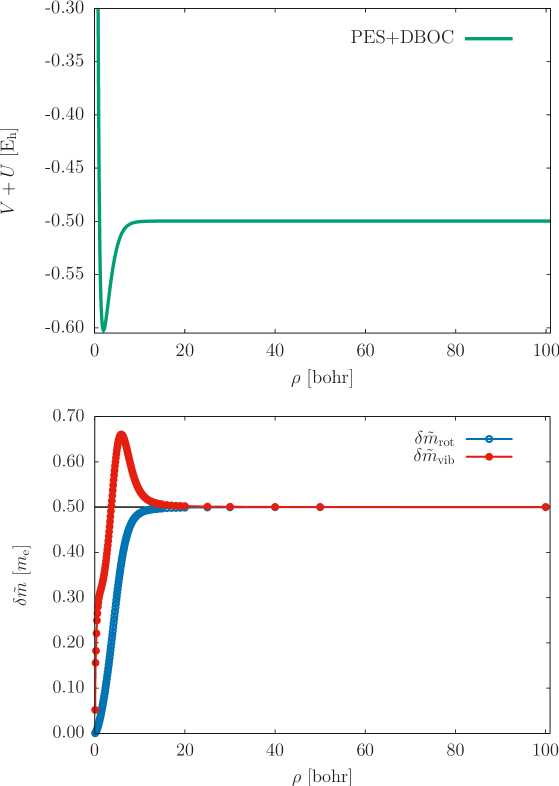
Figure 1: H${}_{2}^{+}$ molecular ion in its $\tilde{X}\ {{}^{2}\Sigma}_{\text{g}}^{+}$ electronic state (ground state): mass correction functions to the vibrational, $\delta\tilde{m}_{\text{vib}}=\mathcal{A}^{\rho}\,_{\rho}$, and the rotational, $\delta\tilde{m}_{\text{rot}}=\mathcal{A}^{\theta}\,_{\theta}=\mathcal{A}^{\phi}\,_{\phi}$ degrees of freedom when the kinetic energy operator is expressed in spherical polar coordinates, Eq. (180). For the definition of the effective rotational and vibrational mass in diatomic molecules see Eqs. (237)–(240). The thin line takes the constant value $1/2=0.5\ m_{\text{e}}$, which corresponds to an equal share of the single electron between the two atomic nuclei.

Table 1: Non-adiabatic corrections for the rovibrational states of H${}_{2}^{+}$: comparison (deviation) from Moss’ results (computed with $m_{\text{p}}/m_{\text{e}}=1836.152701$ and $1~{}\text{E}_{\text{h}}=219474.63067$ cm^-1) Moss (1993, 1996).

$v$/$J$	0	1	2	3	4	5	6	7	8	9	10	11	12	13	14	15	16	17	18	19	20
0	$-0.002$	$-0.002$	0.059${}^{\text{a}}$	$-0.002$	$-0.001$	$0.000$	$-0.001$	$-0.001$	$-0.002$	$-0.002$	$-0.004$	$-0.002$	$-0.003$	$-0.003$	$-0.002$	$-0.002$	$-0.003$	$-0.003$	$-0.002$	$-0.002$	$-0.003$
1	$0.000$	$-0.002$	$-0.003$	$-0.002$	$-0.002$	$0.000$	$-0.001$	$-0.002$	$-0.002$	$-0.002$	$-0.002$	$-0.003$	$-0.001$	$-0.002$	$-0.002$	$-0.002$	$-0.003$	$-0.002$	$-0.003$	$-0.003$	$-0.003$
2	$-0.002$	$-0.002$	$-0.003$	$-0.001$	$-0.002$	$-0.001$	$-0.003$	$-0.002$	$-0.001$	$-0.002$	$-0.002$	$-0.002$	$-0.002$	$-0.003$	$-0.003$	$-0.003$	$-0.003$	$-0.002$	$-0.002$	$-0.003$	$-0.003$
3	$-0.002$	$-0.003$	$-0.002$	$-0.002$	$-0.002$	$-0.002$	$-0.003$	$-0.001$	$-0.002$	$-0.003$	$-0.003$	$-0.002$	$-0.002$	$-0.002$	$-0.003$	$-0.003$	$-0.003$	$-0.003$	$-0.003$	$-0.003$	$-0.003$
4	$-0.002$	$-0.002$	$-0.002$	$-0.003$	$-0.002$	$-0.003$	$-0.002$	$-0.002$	$-0.002$	$-0.002$	$-0.003$	$-0.003$	$-0.003$	$-0.003$	$-0.003$	$-0.002$	$-0.003$	$-0.003$	$-0.003$	$-0.003$	$-0.002$
5	$-0.002$	$-0.003$	$-0.003$	$-0.003$	$-0.003$	$-0.002$	$-0.002$	$-0.003$	$-0.002$	$-0.003$	$-0.003$	$-0.002$	$-0.003$	$-0.003$	$-0.003$	$-0.003$	$-0.002$	$-0.003$	$-0.003$	$-0.003$	$-0.002$
6	$-0.003$	$-0.002$	$-0.002$	$-0.003$	$-0.002$	$-0.003$	$-0.003$	$-0.003$	$-0.002$	$-0.003$	$-0.003$	$-0.003$	$-0.002$	$-0.002$	$-0.003$	$-0.003$	$-0.003$	$-0.003$	$-0.003$	$-0.003$	$-0.003$
7	$-0.003$	$-0.003$	$-0.004$	$-0.003$	$-0.003$	$-0.002$	$-0.003$	$-0.004$	$-0.003$	$-0.003$	$-0.002$	$-0.003$	$-0.003$	$-0.003$	$-0.003$	$-0.003$	$-0.002$	$-0.003$	$-0.003$	$-0.002$	$-0.002$
8	$-0.002$	$-0.003$	$-0.003$	$-0.003$	$-0.003$	$-0.003$	$-0.003$	$-0.003$	$-0.003$	$-0.003$	$-0.003$	$-0.003$	$-0.003$	$-0.003$	$-0.002$	$-0.003$	$-0.002$	$-0.002$	$-0.002$	$-0.002$	$-0.002$
9	$-0.003$	$-0.003$	$-0.003$	$-0.003$	$-0.003$	$-0.002$	$-0.002$	$-0.002$	$-0.003$	$-0.003$	$-0.003$	$-0.002$	$-0.002$	$-0.002$	$-0.002$	$-0.003$	$-0.002$	$-0.002$	$-0.001$	$-0.001$	$-0.002$
10	$-0.003$	$-0.002$	$-0.003$	$-0.003$	$-0.273$${}^{\text{b}}$	$-0.003$	$-0.002$	$-0.003$	$-0.003$	$-0.002$	$-0.002$	$-0.002$	$-0.002$	$-0.002$	$-0.002$	$-0.002$	$-0.002$	$-0.001$	$-0.001$	$-0.001$	$-0.002$
11	$-0.002$	$-0.002$	$-0.003$	$-0.003$	$-0.002$	$-0.002$	$-0.002$	$-0.003$	$-0.002$	$-0.003$	$-0.002$	$-0.001$	$-0.002$	$-0.001$	$-0.001$	$-0.001$	$-0.002$	$-0.002$	$-0.001$	$-0.001$	$-0.001$
12	$-0.002$	$-0.002$	$-0.002$	$-0.002$	$-0.002$	$-0.003$	$-0.002$	$-0.002$	$-0.003$	$-0.002$	$-0.001$	$-0.001$	$-0.002$	$-0.002$	$-0.002$	$-0.001$	$-0.001$	$-0.001$	$-0.001$	$\bullet$
13	$-0.002$	$-0.002$	$-0.002$	$-0.002$	$-0.002$	$-0.002$	$-0.002$	$-0.002$	$-0.002$	$-0.002$	$-0.002$	$-0.002$	$-0.001$	$-0.001$	$-0.001$	$-0.001$	$-0.001$	$\bullet$
14	$-0.001$	$-0.002$	$-0.002$	$-0.002$	$-0.001$	$-0.001$	$-0.002$	$-0.001$	$-0.001$	$-0.002$	$-0.001$	$-0.001$	$-0.001$	$0.000$	$-0.001$	$\bullet$
15	$-0.001$	$-0.002$	$-0.001$	$-0.002$	$-0.001$	$-0.001$	$-0.001$	$-0.001$	$-0.001$	$-0.001$	$-0.001$	$-0.001$	$0.002$	$\bullet$
16	$-0.001$	$-0.001$	$-0.001$	$-0.002$	$-0.001$	$-0.001$	$-0.001$	$-0.001$	$-0.001$	$0.001$	$\bullet$
17	$-0.001$	$0.000$	$-0.001$	$-0.001$	$-0.001$	$-0.001$	$0.000$	$\bullet$
18	$0.000$	$0.000$	$0.000$	$0.000$	$\bullet$
19	$0.000$	$0.000$
$v$/$J$	21	22	23	24	25	26	27	28	29	30	31	32	33	34	35	36	37	38	39	40	41
0	$-0.003$	$-0.003$	$-0.003$	$-0.002$	$-0.003$	$-0.003$	$-0.004$	$-0.003$	$-0.003$	$-0.004$	$-0.003$	$-0.004$	$-0.004$	$-0.004$	$-0.004$	$-0.003$	$-0.003$	$-0.003$	$-0.003$	$-0.001$	$\bullet$
1	$-0.003$	$-0.003$	$-0.003$	$-0.003$	$-0.003$	$-0.003$	$-0.003$	$-0.003$	$-0.003$	$-0.003$	$-0.003$	$-0.003$	$-0.004$	$-0.003$	$-0.003$	$-0.003$	$-0.003$	$0.006$	$\bullet$
2	$-0.002$	$-0.004$	$-0.003$	$-0.003$	$-0.004$	$-0.003$	$-0.003$	$-0.003$	$-0.003$	$-0.004$	$-0.003$	$-0.003$	$-0.003$	$-0.003$	$-0.003$	$-0.002$	$-0.193$${}^{\text{e}}$	$\bullet$
3	$-0.003$	$-0.002$	$-0.003$	$-0.003$	$-0.003$	$-0.003$	$-0.003$	$-0.003$	$-0.003$	$-0.003$	$-0.002$	$-0.002$	$-0.002$	$-0.002$	$0.047$${}^{\text{d}}$	$\bullet$
4	$-0.003$	$-0.004$	$-0.003$	$-0.003$	$-0.003$	$-0.003$	$-0.003$	$-0.002$	$-0.002$	$-0.002$	$-0.002$	$-0.002$	$0.003$	$\bullet$
5	$-0.003$	$-0.002$	$-0.003$	$-0.002$	$-0.002$	$-0.002$	$-0.002$	$-0.002$	$-0.002$	$-0.002$	$0.006$	$\bullet$
6	$-0.002$	$-0.003$	$-0.002$	$-0.002$	$-0.002$	$-0.002$	$-0.002$	$-0.001$	$-0.002$	$\bullet$
7	$-0.002$	$-0.002$	$-0.002$	$-0.001$	$-0.002$	$-0.002$	$-0.002$	$0.018$${}^{\text{c}}$	$\bullet$
8	$-0.002$	$-0.002$	$-0.001$	$-0.001$	$-0.001$	$0.005$	$\bullet$
9	$-0.001$	$-0.001$	$-0.001$	$-0.001$	$\bullet$
10	$-0.001$	$-0.001$	$\bullet$
11	$\bullet$
${}^{\text{a,b}}$ The stability and estimated accuracy of our correction terms is much better than the order of magnitude of the deviation.
${}^{\text{c,d,e}}$ The accuracy of these results has been labelled in the present work as well as Ref. Moss (1993). The symbol $\bullet$ is used for states which have been predicted
by Moss without giving their energy and non-adiabatic correction explicitly in Refs. Moss (1993, 1996).

VII Summary and conclusions

General curvilinear expressions have been derived for the second-order non-adiabatic kinetic energy operator. The derivations have been carried out using the general Jacobian and metric tensors of the coordinate transformation, thereby they are in direct connection with the numerical-kinetic energy operator approach (with constant masses) also used in the GENIUSH protocol Mátyus et al. (2009). While for the constant-mass case one has to transform the “div grad” operator to curvilinear coordinates, we had to consider the “div $\mathcal{M}$ grad” operator with the $\mathcal{M}$ coordinate-dependent tensor quantity within the operator. As a result, should a general mass-correction tensor surfaces become available for polyatomic molecules, their implementation in the (polyatomic) rovibrational GENIUSH program has been made straightforward.

At the moment, we are not aware of any widely available electronic structure package which we could use to compute the mass-correction tensor over a wide range of nuclear configurations of polyatomic molecules (note however that Ref. Scherrer et al. (2017) points into a very promising direction). Hence, we have modified (simplified) our in-house preBO code originally developed for the computation of isolated few-particle quantum systems Mátyus et al. (2011a, b); Mátyus and Reiher (2012); Mátyus (2013, 2018) to few-electron systems being in interaction with external charges (nuclei) and use floating explicitly-correlated Gaussian functions for the spatial part of the basis set. We report the first numerical results using this computational setup and present the rigorous mass-correction values for the H${}_{2}^{+}$ molecular ion in its ground electronic state over the $[0.1,100]$ bohr range of the internuclear distance. Using these mass-correction functions in the rovibrational computations we reproduce Moss’ non-adiabatic corrections Moss (1993, 1996) for H${}_{2}^{+}$ within a few 0.001 cm^-1 for the bound and long-lived resonance states. In a forthcoming paper Ma (1) further applications of the developed formalism and methodology are presented for the ⁴He${}_{2}^{+}$ molecular ion in its ground electronic state for which a highly accurate potential energy and DBOC curve is available Tung et al. (2012). It is observed that full account of the rigorous mass correction functions substantially reduce the deviation of experimental Carrington et al. (1995); Semeria et al. (2016) and computed rotational(-vibrational) energy intervals.

Supplementary Material
The Supplementary Material contains non-adiabatic mass correction values for H${}_{2}^{+}$ ($\tilde{X}\ ^{2}\Sigma_{\text{g}}^{+}$).

Acknowledgment
Financial support of the Swiss National Science Foundation through a PROMYS Grant (no. IZ11Z0_166525) is gratefully acknowledged. The author is thankful to Krzysztof Pachucki for discussions about non-adiabatic perturbation theory, and to Federica Agostini for the explanation of the mass-correction tensor derivation starting from exact factorization.

References

- Fisk and Kirtman (1964) G. A. Fisk and B. Kirtman, J. Chem. Phys. 41, 3516 (1964).
- Bunker and Moss (1977) P. R. Bunker and R. E. Moss, Mol. Phys. 33, 417 (1977).
- Bunker and Moss (1980) P. R. Bunker and R. E. Moss, J. Mol. Spectrosc. 80, 217 (1980).
- Bunker et al. (1977) P. R. Bunker, C. J. McLarnon, and R. E. Moss, Mol. Phys. 33, 417 (1977).
- Schwenke (2001a) D. W. Schwenke, J. Chem. Phys. 114, 1693 (2001a).
- Schwenke (2001b) D. W. Schwenke, J. Phys. Chem. A 105, 2352 (2001b).
- Pachucki and Komasa (2008) K. Pachucki and J. Komasa, J. Chem. Phys. 129, 034102 (2008).
- Pachucki and Komasa (2009) K. Pachucki and J. Komasa, J. Chem. Phys. 130, 164113 (2009).
- Pachucki and Komasa (2012) K. Pachucki and J. Komasa, J. Chem. Phys. 137, 204314 (2012).
- Kutzelnigg (2007) W. Kutzelnigg, Mol. Phys. 105, 2627 (2007).
- Jaquet and Kutzelnigg (2008) R. Jaquet and W. Kutzelnigg, Chem. Phys. 346, 69 (2008).
- Diniz et al. (2013) L. G. Diniz, J. R. Mohallem, A. Alijah, M. Pavanello, L. Adamowicz, O. L. Polyansky, and J. Tennyson, Phys. Rev. A 88, 032506 (2013).
- Weigert and Littlejohn (1993) S. Weigert and R. G. Littlejohn, Phys. Rev. A 47, 3506 (1993).
- Scherrer et al. (2017) A. Scherrer, F. Agostini, D. Sebastiani, E. K. U. Gross, and R. Vuilleumier, Phys. Rev. X 7, 031035 (2017).
- Scherrer et al. (2015) A. Scherrer, F. Agostini, D. Sebastiani, E. K. U. Gross, and R. Vuilleumier, J. Chem. Phys. 143, 074106 (2015).
- Herman and Asgharian (1966) R. M. Herman and A. Asgharian, J. Mol. Spectrosc. 19, 305 (1966).
- Herman and Ogilvie (1998) R. M. Herman and J. F. Ogilvie, Adv. Chem. Phys. 103, 187 (1998).
- Ogilvie (1998) J. F. Ogilvie, The Vibrational and Rotational Spectrometry of Diatomic Molecules (Academic Press, 1998).
- Sauer et al. (2005) S. P. A. Sauer, H. J. A. Jensen, and J. F. Ogilvie, Adv. Quant. Chem. 48, 319 (2005).
- Bak et al. (2005) K. L. Bak, S. P. A. Sauer, J. Oddershede, and J. F. Ogilvie, Phys. Chem. Chem. Phys. 7, 1747 (2005).
- Braun et al. (1996) P. A. Braun, T. K. Rebane, and K. Ruud, Chem. Phys. 208, 299 (1996).
- Panati et al. (2007) G. Panati, H. Spohn, and S. Teufel, ESAIM: Mathematical Modelling and Numerical Analysis 41, 297 (2007).
- Semeria et al. (2016) L. Semeria, P. Jansen, and F. Merkt, J. Chem. Phys. 145, 204301 (2016).
- Ma (1) E. Mátyus, Computation of the non-adiabatic mass-correction functions and rovibrational energy levels for the 4He molecular ion in its ground electronic state, J. Chem. Phys. accepted (2018).
- Handy and Lee (1996) N. C. Handy and A. M. Lee, Chem. Phys. Lett. 252, 425 (1996).
- Ioannou et al. (1996) A. G. Ioannou, R. D. Amos, and N. C. Handy, Chem. Phys. Lett. 251, 52 (1996).
- Handy et al. (1986) N. C. Handy, Y. Yamaguchi, and H. F. Schaefer III, J. Chem. Phys. 84, 4481 (1986).
- Cencek and Kutzelnigg (1997) W. Cencek and W. Kutzelnigg, Chem. Phys. Lett. 266, 383 (1997).
- Kutzelnigg (1997) W. Kutzelnigg, Mol. Phys. 90, 909 (1997).
- Mátyus et al. (2009) E. Mátyus, G. Czakó, and A. G. Császár, J. Chem. Phys. 130, 134112 (2009).
- Mátyus and Reiher (2012) E. Mátyus and M. Reiher, J. Chem. Phys. 137, 024104 (2012).
- Mátyus (2013) E. Mátyus, J. Phys. Chem. A 117, 7195 (2013).
- Mátyus (2018) E. Mátyus, Mol. Phys. p. arXiv:1801.05885 (2018).
- Tennyson (2016) J. Tennyson, J. Chem. Phys. 145, 120901 (2016).
- Carrington Jr. (2017) T. Carrington Jr., J. Chem. Phys. 146, 120902 (2017).
- Luckhaus (2000) D. Luckhaus, J. Chem. Phys. 113, 1329 (2000).
- Lauvergnat and Nauts (2002) D. Lauvergnat and A. Nauts, J. Chem. Phys. 116, 8560 (2002).
- Podolsky (1928) B. Podolsky, Phys. Rev. 32, 812 (1928).
- Fábri et al. (2011) C. Fábri, E. Mátyus, and A. G. Császár, J. Chem. Phys. 134, 074105 (2011).
- Sarka et al. (2016) J. Sarka, A. G. Császár, S. C. Althorpe, D. J. Wales, and E. Mátyus, Phys. Chem. Chem. Phys. 18, 22816 (2016).
- Sarka et al. (2017) J. Sarka, A. G. Császár, and E. Mátyus, Phys. Chem. Chem. Phys. 19, 15335 (2017).
- Suzuki and Varga (1998) Y. Suzuki and K. Varga, Stochastic Variational Approach to Quantum-Mechanical Few-Body Problems (Springer-Verlag, Berlin, 1998).
- Po (0) M. J. D. Powell, The NEWUOA software for unconstrained optimization without derivatives (DAMTP 2004/NA05), Report no. NA2004/08, http://www.damtp.cam.ac.uk/user/na/reports04.html last accessed on January 18, 2013.
- Pavanello et al. (2012) M. Pavanello, L. Adamowicz, A. Alijah, N. F. Zobov, I. I. Mizus, O. L. Polyansky, T. S. J. Tennyson, and A. G. Császár, J. Chem. Phys. 136, 184303 (2012).
- Jaquet and Khoma (2017) R. Jaquet and M. Khoma, J. Phys. Chem. A 121, 7016 (2017).
- Jaquet and Khoma (2018) R. Jaquet and M. V. Khoma, Mol. Phys. p. doi.org/10.1080/00268976.2018.1464225 (2018).
- Moss (1993) R. E. Moss, Mol. Phys. 80, 1541 (1993).
- Moss (1996) R. E. Moss, Mol. Phys. 89, 195 (1996).
- Korobov (2018) V. I. Korobov, Mol. Phys. 116, 93 (2018).
- Beyer and Merkt (2016a) M. Beyer and F. Merkt, Phys. Rev. Lett. 116, 093001 (2016a).
- Beyer and Merkt (2016b) M. Beyer and F. Merkt, J. Mol. Spectrosc. 330, 147 (2016b).
- Pachucki and Komasa (2018) K. Pachucki and J. Komasa, Phys. Chem. Chem. Phys. 20, 247 (2018).
- Mátyus et al. (2011a) E. Mátyus, J. Hutter, U. Müller-Herold, and M. Reiher, Phys. Rev. A 83, 052512 (2011a).
- Mátyus et al. (2011b) E. Mátyus, J. Hutter, U. Müller-Herold, and M. Reiher, J. Chem. Phys. 135, 204302 (2011b).
- Tung et al. (2012) W.-C. Tung, M. Pavanello, and L. Adamowicz, J. Chem. Phys. 136, 104309 (2012).
- Carrington et al. (1995) A. Carrington, C. H. Pyne, and P. J. Knowles, J. Chem. Phys. 102, 5979 (1995).