Encoding-side-channel-free and measurement-device-independent quantum key distribution

Abstract

We present a simple protocol where Alice and Bob only needs sending out a coherent state or not-sending out a coherent state to Charlie. There is no bases switching. We show that this protocol is both encoding-state-side-channel free to the source part and measurement-device-independent. We don’t have to control exactly the whole space state of the light pulse, which is an impossible task in practice. The protocol is immune to all adverse due to encoding-state imperfections in side-channel space such as the photon frequency spectrum, emission time, propagation direction, spatial angular moment, and so on. Numerical simulation shows that our scheme can reach a side-channel-free result for quantum key distribution over a distance longer than 200 km given the single-photon-interference misalignment error rate of $20\%$.

I Introduction Guaranteed by principles of quantum mechanics, quantum key distribution (QKD) can provide a secure key for private communication BB84 ; GRTZ02 even though Eve can completely control the channel. However, there are side-channel effects due to the device imperfections in practiceILM ; H03 ; wang05 ; LMC05 ; wangyang ; njp ; PNS ; PNS1 . In general, we can divide the whole space of an encoding state from a real source into two subspaces, the operational space and the side channel space. Even though the source state encoding looks perfect when it is examined in the operational space, there could be security loopholes due to imperfections in the side channel space, this is what we called side-channel effects. For example, in the BB84 protocolBB84 , even though a perfect single-photon source is applied, there are still some side-channel effects which can undermine the security assumed in the operational space. There could be basis-dependent synchronization errors in pulse emitting time or frequency spectrum difference for different encoding states or bases and Eve can make use of this to judge the basis or encoding state chosen in a certain time window. In general, all encoding states from the source live in an infinite dimensional space which is formed by the operational space and the side-channel space. Though we only use the encoding space (e.g., polarization) for QKD, Eve can do his attack in side-channel space such as frequency space to obtain information. Given the inevitable imperfections in the side-channel space for the encoding states, Eve can make use of these and obtain information without causing any change to the Alice and Bob’s observation outcome in the operation space. As we shall show latter, given a lossy channel, by taking side channel attacks to the source, Eve can actually almost obtain full information of a QKD result without disturbing the encoding states in the operational space. Here we propose a QKD scheme that is both source encoding-state-side-channel-free and measurement device independent (MDI)curty1 ; ind3 ; wang10 . Although some existing protocols can also achieve the goal of side-channel-free security ind1 ; ind3 , our protocol presented here is the only one that bases on the matured existing technologies and there is no demanding on the local detection efficiency.

Our protocol is not source device independent. The so called encoding-state-side-channel free means that we don’t worry about any information leakage from the side-channel space of the encoded states. We do have conditions in the operational space. In this work we assume that the encoding states from the source behave perfectly when they are measured in the operational space, but can be imperfect in the side-channel space. Hopefully, the condition on the operational space can be loosened in the future. Actually, there are lots of studies on security with inexact encoding stateswangyang ; njp ; wang10 ; ind2 in the operational space. On the other hand, doing calibration only in the operational space seems to be much easier than that in the whole space, which seems to be an impossible task in practice. Also, our protocol is side-channel free for the encoding states only. It assumes no information leakage due to other hidden accesses beyond the sent-out encoding states. Say, the source has no hidden classical information leakage. Note that in the existing device-independent protocols, there are also similar assumed conditions for security, although the conditions are on the measurement devices rather than the encoding states. Since our protocol is measurement device independent, there is no condition on the measurement devices for security. The security of our protocol is obviously stronger than the normal MDI-QKD because there is no security loophole in the encoding states of our protocol. Compared with the existing device-independent QKD, our protocol has a drawback in that it is not entirely source-independent, but it has an advantage of measurement-device-independent. Note that the device independent QKD is not MDI, because it requests no information leakage of the measurement outcome. Most importantly, our protocol only rely on matured technologies and it can achieve a meaningful secure distance, a distance longer than 200 kilometers even though the misalignment error rate is as large as 20%.

II Some side-channel attacks and Theorem 1. Consider a two-basis QKD protocol, such as the BB84 protocol, where there are $X$ basis and $Z$ basis in the protocol. Suppose we take state-encoding in the photon polarization space and we regard the polarization space as the operational space. In the existing methods in generating the different encoding states, we need either use different diodes to generate different encoding states or use only one diode together with randomly chosen modulations, such as flipping, rotation, phase shift, etc. These operations can cause differences in the side channel space. In particular, the frequency spectrums can be a little bit different for different encoding states or different bases. In principle, by detecting frequency difference, Eve has a chance to know which encoding state is used in the operational space and she will cause no change to the states in operational space. As another example, if different encoding states are actually emitted at different time, Eve may just measure the photon with a very precise clock and she can sometimes know the coding state almost exactly if the photon wave packet collapses at certain time intervals. Also, Eve may make use of the channel loss, she can choose to block all those photons on which the side-channel attack done by her is not successful. Thus, small bias of a state in the side-channel space may flaw the whole protocol.

Fortunately, the ideal source is not the only secure source. A real-life source is secure if it can be mapped from an ideal source. Suppose in a certain protocol $\mathcal{K}$ requests $k$ different encoding states. For example, in the BB84 protocol, we need 4 encoding states. Perfect source $\mathcal{P}$ always produces a perfect encoding state in every time window and all states are identical in the side channel space. An imperfect source produces non-ideal encoding states in the whole space, with imperfections in the side-channel space and the states in side-channel space can change from time to time. Say, at a certain time window, the imperfect source produces the $k$ encoding states in the whole space and we name them as set $\mathcal{S}_{i}$. We then randomly choose one from $\mathcal{S}_{i}$ and send it out for QKD. If there is always a (time-dependent) quantum process $\mathcal{M}_{i}$ that maps the $k$ perfect states to the corresponding $k$ non-ideal states in set $\mathcal{S}_{i}$, then we say source $\mathcal{S}$ can be mapped from a perfect source $\mathcal{P}$.
Theorem 1 In any QKD protocol, a real-life source $\mathcal{S}$ emitting imperfect states in the whole space is equivalent to a perfect (virtual) source $\mathcal{P}$ emitting perfect states which are all identical in side channel space if there exists a quantum process $\mathcal{M}$ that can map source $\mathcal{P}$ to source $\mathcal{S}$. The final key of a QKD protocol using source $\mathcal{S}$ can be calculated by assuming that the virtual source $\mathcal{P}$ were used.

This conclusion is rather obvious. Suppose $\mathcal{S}$ is insecure, then in a QKD protocol where the ideal source $\mathcal{P}$ is applied, Eve can first use the quantum process $\mathcal{M}$ to transform it into source $\mathcal{S}$ and then attack the QKD protocol as if the protocol used source $\mathcal{S}$. This means that if $\mathcal{S}$ is not secure then $\mathcal{P}$ is not secure either. Here in the theorem above, the quantum process $\mathcal{M}$ is not limited to a unitary process, although in showing the side-channel free property of our protocol we mainly use a unitary map.
III Our protocol
In our protocol, we use the idea of twin-field QKD (TFQKD)nature18 with the classical bit value encoding done by the decisions of sending or not-sending made by Alice and Bob. The schematic picture of side-channel-free QKD is shown in Fig. 1.

Figure 1: Schematic picture of side-channel-free QKD.

Our protocol is different from wxb in that we directly use the whole non-random-phase coherent states. There are 3 parties, Alice, Bob, and the third party Charlienature18 . They (Alice and Bob) will use coherent states and vacuum only. We first present our protocol in the operational space only and then show why it is side-channel free using our Theorem 1.
Protocol R, real protocol
R-1 At any time window $i$, Alice (Bob) always prepare a coherent state $|\alpha_{A}\rangle=\sum_{n=0}^{\infty}\frac{e^{-\mu/2}{\mu}^{n/2}e^{in\gamma_{A}}}{\sqrt{n!}}$ ($|\alpha_{B}\rangle=\sum_{n=0}^{\infty}\frac{e^{-\mu/2}{\mu}^{n/2}e^{in\gamma_{B}}}{\sqrt{n!}}$) and announces the states, including the global phases $\gamma_{A},\gamma_{B}$. With a probability $q$ Alice (Bob) decides sending, and with a probability $1-q$ she (he) decides not-sending. If she (he) decides sending, she (he) sends out the coherent state $|\alpha_{A}\rangle$ ($|\alpha_{B}\rangle$) to Charlie and puts down a classical bit value $1$ ($0$) locally; if she (he) decides not-sending she (he) does not send out anything, i.e., she (he) sends out a vacuum to Charlie and puts down a classical bit value $0$ ($1$) locally.
R-2 Charlie announces his measurement outcome and hence determines the effective events: an event with one and only one detector clicking announced by Charlie. A time window or classical bit value corresponding to an effective event is named as an effective time window or effective bit.
Definition $\tilde{Z}$-window: A time window when Alice decides sending and Bob decides not-sending, or Alice decides not-sending and Bob decides sending.
R-3 Through classical communication, they take a random subset of time windows $v$ to test the bit-flip error rate; they take another random subset of time windows $u$ to verify the upper bound value of phase-flip error rate $\bar{e}^{ph}$ of the effective bits corresponding to $\tilde{Z}$-windows, those time windows when one party from Alice and Bob decides sending and the other party decides not-sending. They discard effective bits from $v$-windows or $u$-windows after error test.
R-4 They distill (by taking error correction and privacy amplification to ) the remaining effective bits after error test, with the asymptotic result for number of final bits:

$$n_{F}=n_{\tilde{Z}}-n_{\tilde{Z}}H(\bar{e}^{ph})-fn_{t}H(E_{Z})$$ (1)

where the entropy functional $H(x)=-x\log_{2}x-(1-x)\log_{2}(1-x)$; $n_{\tilde{Z}}$ ($n_{t}$) is the number of remaining effective bits from $\tilde{Z}$-windows (all time windows) after error test; $f$ is the correction efficiency factor.
Note 1 The encoding is done by decisions on sending or not-sending made by Alice and Bob. More precisely, the sending or not-sending decision of a time window always corresponds to the local classical bits $1$, $0$ to Alice, or 0, 1 to Bob. We can also imagine that whenever Alice (Bob) decides sending or not-sending, she (he) always produces a local ancillary photon-number state $|1\rangle$ or $|0\rangle$ and the corresponding bit values are encoded in the local ancillary state. To Alice (Bob), state $|0\rangle$ corresponds to a bit value 0 (1) and state $|1\rangle$ corresponds to a bit value 1 (0). This is equivalent to say that they (Alice and Bob) have used an extended state including real-photon state which will be sent out to Charlie and ancillary state placed locally. For example, in a certain window when Alice decides sending and Bob decides not sending, we can imagine that they have actually prepared an extended state

$$\left(\rho_{A}\cdot|0\rangle\langle 0|\right)\otimes|10\rangle\langle 10|.$$ (2)

where $\rho_{A}=|\alpha_{A}\rangle\langle\alpha_{A}|$. The real-photon state $\rho_{A}\cdot|0\rangle\langle 0|$ will be sent out to Charlie. In this paper, we shall name the state left to the tensor-product symbol $\otimes$ as the real-photon state, and the state right to the tensor-product symbol $\otimes$ as the ancillary-photon state. As stated already, each one’s bit value is actually encoded in the local ancillary photon-number state.
Note 2 The bit-flip error and phase-flip error. Bob makes a wrong bit encoding if his bit value is different from Alice’s bit value at a certain time window. To every event in the subset $v$ randomly taken by them, they announce each one’s bit values (decision on sending or not-sending) to judge the bit-flip error rate. Also, as shown in the Appendix, using the details of events in set $v$, they can calculate the phase-flip error rate $\bar{e}^{ph}$ by Eq.(11).
Note 3 Charlie’s compensation. To obtain a good key rate, they need a low phase-flip error rate. In the protocol, an event of right-detector clicking due to the real-photon state $|\alpha_{A}\rangle\otimes|\alpha_{B}\rangle=|\sqrt{\mu}e^{i\gamma_{A}}\rangle\otimes|\sqrt{\mu}e^{i\gamma_{B}}\rangle$ will contribute to the phase-flip errors. The states $|\alpha_{A}\rangle$ and $|\alpha_{B}\rangle$ are publicly announced, Charlie can do compensation to remove the global phases $\gamma_{A}$ and $\gamma_{B}$ in the states, so that the clicking detector is very unlikely to be the right detector given the real-photon state $|\alpha_{A}\rangle\otimes|\alpha_{B}\rangle$. Very importantly, as shown in the Appendix, although Charlie’s collaboration can lead to a high key rate, the security of the protocol does not rely on Charlie’s honesty.
Note 4 Why it is side-channel free ? Intuitively speaking, our protocol takes no physical-bases switching. Other protocols, such as the BB84, MDIQKD protocol, the TFQKD, and so on, they all need to take modulation to the outcome states differently in switching between different bases. We can give a strict proof for the side-channel free property of our protocol. Here we show directly by our Theorem 1 that the protocol R is side channel free, say, if it is secure in operational space, it must be also secure in the whole space including the side channel space. Later in the appendix we present the measurement-device-independent security proof of the protocol itself in operational space only, i.e., in the case we don’t consider any side-channel effects. Here we only need to show that the protocol is the encoding-state-side-channel free. In step R-1, they try to prepare a coherent state $|\alpha_{A}\rangle$, $|\alpha_{B}\rangle$ in the operational space. In the ideal case we don’t need to consider the side-channel space. For example, in the case that any Fock state $|n\rangle$, no matter it is from Alice’s state $|\alpha_{A}\rangle$ or from Bob’s state $|\alpha_{B}\rangle$, are identical in side-channel space. So, we shall just use the original notations of $|\alpha_{A}\rangle$ and $|\alpha_{B}\rangle$ to represent the ideal whole-space state. However, what is actually prepared in a real experiment must have imperfections in the side-channel space. But the vacuum state has no side channel space therefore we only need to consider side-channel-space for the non-vacuum parts in each coherent state. Say, $|\alpha_{x}\rangle=e^{-\mu/2}|0\rangle+\sqrt{1-e^{-\mu}}|\tilde{\alpha}_{x}\rangle$and $\sqrt{1-e^{-\mu}}|\tilde{\alpha}_{x}\rangle=|\alpha_{x}\rangle-e^{-\mu/2}|0\rangle$ where $x$ can be $A,B$. We only need consider the whole-space state of $|\tilde{\alpha}_{x}\rangle$. Therefore, we need to consider the corresponding whole-space states in the following form instead of the ideal states:

$$|0\rangle \longrightarrow|0\rangle$$

$$|\alpha_{A}\rangle \longrightarrow e^{-\mu/2}|0\rangle+\sqrt{1-e^{-\mu}}|\psi_{A}(\tilde{\alpha}_{A})\rangle$$

$$|\alpha_{B}\rangle \longrightarrow e^{-\mu/2}|0\rangle+\sqrt{1-e^{-\mu}}|\psi_{B}(\tilde{\alpha}_{B})\rangle.$$ (3)

Here the states left to the arrow are the ideal states and the states right to the arrow are the corresponding real-life states. States $|\psi_{A}(\tilde{\alpha}_{A})\rangle$ and $|\psi_{B}(\tilde{\alpha}_{B})\rangle$ contain whatever side-channel information such as the frequency spectrum, the polarization, the wave shape, the emission time and so on. We assume Eve exactly knows all these information. These mean, Eve knows all details of the state in the whole space and she can write down the whole-space states exactly and she can make use of it in whatever way she likes. However, consider the form of Eq.(Encoding-side-channel-free and measurement-device-independent quantum key distribution), it is obvious that there exists a unitary operation relates the ideal states and the whole-space states used in the protocol. Note that here we don’t assume errors in the operational space. This means when we assume a non-ideal whole-space state, it must be able to present the same result in the operational space with that of the ideal state. Say, for state $|\psi_{A}(\tilde{\alpha}_{A})\rangle$, if it is measured in photon-number space, it can only present the same probability distribution $P_{n}$ for different photon number states with ideal state $|\tilde{\alpha}\rangle$ result, i.e., $|\langle n|\psi_{A}(\tilde{\alpha}_{A})\rangle|^{2}=|\langle n|\tilde{\alpha}_{A}\rangle|^{2}$. Given this, we immediately know that $\langle 0|\psi_{A}(\tilde{\alpha}_{A})\rangle=\langle 0|\psi_{B}(\tilde{\alpha}_{B})\rangle=0$ Therefore there exists the following unitary transformations:

$$\mathcal{U}_{A}|0\rangle=\mathcal{U}_{B}|0\rangle=|0\rangle \mathcal{U}_{A}|\tilde{\alpha}_{A}\rangle=|\psi_{A}(\tilde{\alpha}_{A})\rangle$$

$$\mathcal{U}_{B}|\tilde{\alpha}_{B}\rangle=|\psi_{B}(\tilde{\alpha}_{B})\rangle$$ (4)

These equations show that the real-life source which emits non-ideal whole-space states can be mapped from an ideal source by two mode unitary transformation $\mathcal{U}_{A}\otimes\mathcal{U}_{B}$. Say, given an ideal two mode source in the protocol, one can simply take unitary transformation $\mathcal{U}_{A}$ to every encoding state from Alice’s ideal physical source and take a unitary transformation $\mathcal{U}_{B}$ to every encoding state from Bob’s ideal physical source, they can in this way obtain all their imperfect states of the real-life source. Applying our Theorem 1, we immediately conclude that our real protocol, protocol R is secure with a real-life source if it is secure with an ideal source.

Obviously, the protocol allows to use a source with unstable side-channel information. Say, at any time window $i$, they have prepared the whole-space candidature states $|\psi_{Ai}(\tilde{\alpha}_{A})\rangle$ and $|\psi_{Bi}(\tilde{\alpha}_{B})\rangle$, we only need to replace the unitary transformation $\mathcal{U}_{A}$ and $\mathcal{U}_{B}$ in Eq.(Encoding-side-channel-free and measurement-device-independent quantum key distribution) by $\mathcal{U}_{Ai}$ and $\mathcal{U}_{Bi}$.
Note 5 Intensity difference does not affect the security. Though we demonstrate the protocol with the condition $|\alpha_{A}|=|\alpha_{B}|=\mu$, however, this condition is not needed for security. We only need that the intensities of all time windows are upper bounded by $\mu$ . Say, at any individual time window $i$, we have $|\alpha_{Ai}|=\sqrt{\mu_{Ai}}\leq\sqrt{\mu}$ and $|\alpha_{Bi}|=\sqrt{\mu_{Bi}}\leq\sqrt{\mu}$. All these states can be obtained from an imagined coherent state of intensity $\mu$ by attenuation. Again, applying our Theorem 1 we can assume that they are using coherent states with stable and exact intensity $\mu$apl .
Discussions: Revised protocol by post selection. In the protocol, to produce a good key rate, we need Charlie take phase compensation effectively. Technically, we can further simplify the protocol without such type of active operation. Instead, Alice and Bob can do post selection, they only use those effective events whose corresponding initially prepared state $|\alpha_{A}\rangle=|\sqrt{\mu}e^{i\gamma_{A}}\rangle$, $|\alpha_{B}\rangle=|\sqrt{\mu}e^{i\gamma_{B}}\rangle$ in the time window satisfying

$$1-|\cos(\gamma_{B}-\gamma_{A})|\leq|\lambda|.$$ (5)

If we take a very small $|\lambda|$ value, the phase-flip error rate will be small, though the data size is also small.

Though the protocol presented above is source-side-channel free, it is no entirely source-independent, such as those device-independent protocols ind1 and the protocol shown inind3 . Our protocol takes no assumption for the side channel space, but it has conditions in the operational space. The security proof in its present form assumes an exact vacuum and the sub-Poisson distribution in Fock space for the coherent state. Possibly, these conditions can be loosened through the worst-case study in the future. However we believe even in its present form it has obvious advantages in security already.
Numerical simulation. Assume detector dark count rate to be $10^{-11}$ with detection efficiency of $80\%$, a linear lossy channel with transmittance $\eta=0.1^{-L/100km}$, and the correction efficiency is $f=1.1$. The results of numerical simulation are shown in Fig. 2.

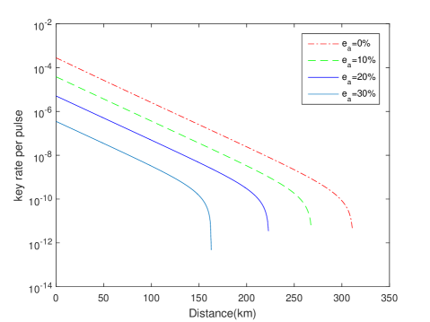
Figure 2: Log scale of the key rate as a function of the distance between Alice and Bob with different misalignment error rate. $e_{a}$: single-photon misalignment error.

Appendix

.1 Outline

There are two parts for the security proof here. Part 1 includes virtual protocols and reduction. In part 1, through virtual protocols and reductions that we first show the security if they only used $\tilde{Z}$-windows. In a real protocol, they sometimes use $\tilde{Z}$-windows and sometimes use other time windows. We regard effective bits from $\tilde{Z}$-windows as un-tagged bits and the effective bits from other time windows as tagged bits. Applying the tagged modelgllp we can obtain the key rate formula as Eq.(1). In the formula, we need two parameters, the bit-flip error rate and the phase-flip error rate. A bit-flip error is the case that Alice and Bob have different values for an effective bit. Therefore the bit-flip error rate can be directly tested by the subset $v$. The phase-flip error is originally defined on the phase-flip rate of virtual ancillary photons. Which can be verified by observing the effective events of $X$-windows in a virtual protocol, heralded by different detectors (left-detector, $L$, or right detector, $R$). The $X$-windows in a virtual protocol contains two subsets, an $X_{+}$-window that sends out a real-photon state $\rho_{+}=|\chi^{+}\rangle\langle\chi^{+}|$ and an $X_{-}$-window that sends out a real-photon state $\rho_{-}=|\chi^{-}\rangle\langle\chi^{-}|$ and

$$|\chi^{\pm}\rangle=(|0,\alpha_{B}\rangle\pm|\alpha_{A},0\rangle)/\mathcal{N}_{\pm}$$ (6)

where $1/\mathcal{N}_{\pm}$ are normalization factors for states $|\chi^{\pm}\rangle$. In our virtual protocol, they set a probability ${|\mathcal{N}_{+}|^{2}}/4$ for an $X_{+}$-window and a probability ${|\mathcal{N}_{-}|^{2}}/4$ for an $X_{-}$-window whenever they use an $X$-window. The sent out states of an $X$-window is

$$\rho_{X}=|\mathcal{N}_{+}|^{2}{\rho_{+}}/4+|\mathcal{N}_{-}|^{2}{\rho_{-}}/4.$$ (7)

As shall be shown, the phase flip error rate is

$$e^{ph}=\frac{n^{R}_{X_{+}}+n^{L}_{X_{-}}}{n_{X}}=\frac{n^{R}_{X_{+}}+n^{L}_{X}-n^{L}_{X_{+}}}{n_{X}}$$

$$\leq\bar{e}^{ph}=\frac{\bar{n}^{R}_{X_{+}}+n^{L}_{X}-{\underline{n}}^{L}_{X_{+}}}{n_{X}}$$ (8)

where $n^{d}_{a}$ is the number of effective $X$-windows heralded by joint events of $d$ and $a$, and $d=L,R$, $a=X_{+},X_{-},X$; and $n_{X}=n_{X}^{L}+n_{X}^{R}$. Event $d$: Charlie announces that detector $d$ has clicked and the other detector has not click. Event $a$: it is a time window of $a$. However, in a real protocol, we don’t have such a state, and hence we have no way to obtain the value by direct observation. But we can still verify the upper bound of the phase-flip error rate by observing data of other states in the real protocol with calculation formulas presented in Part 2. Say, in the real protocol, they randomly take two subsets of all time windows, $v$ and $u$. Details on sending or not-sending of $u$ are never announced. But we know that set $u$ contains a number of $\tilde{Z}$ windows whose density operator is

$$\rho_{\tilde{Z}}=\frac{1}{2}(|0,\alpha_{B}\rangle\langle|0,\alpha_{B}|+|\alpha_{A},0\rangle\langle\alpha_{A},0|)$$ (9)

Obviously, the density operator has another equivalent convex and

$$\rho_{\tilde{Z}}=\rho_{X}$$ (10)

This means, in a virtual protocol, if we don’t announce any information on sending or not-sending of time windows in set $u$, to Eve, those $\tilde{Z}$-windows in set $u$ are identical to $X$-windows. Say, in a real protocol, set $u$ contains fake $X$-windows which are identical to true $X$-windows to Eve. We can then verify the value of $\bar{e}^{ph}$ of fake $X$-windows by observing and calculating the data of another subset of time windows, set $v$ in the real protocol. Explicitly, as shall be shown in part 2, we need the following data in the calculation:
1, The $d$-event rate of time windows $A$, denoted by $S^{d}_{A}$. It is just the fraction of effective time windows heralded by event $d$ from $A$-windows. Here $d=L,R$, for an effective event of detector $d$ clicking and the other detector not clicking as announced by Charlie. We need the values of $S^{d}_{A}$ for $d=L,R$ and $A=\tilde{Z},\mathcal{B},\mathcal{O}$, where $\mathcal{B}$ is for a time window when both Alice and Bob decide sending, and $\mathcal{O}$ is a time window when both Alice and Bob decide not-sending. As shall be shown in Part 2, based on these observed data, we can then calculate the upper bound of phase-flip error rate, $\bar{e}^{ph}$. Explicitly

$$e^{ph}\leq\overline{e}^{ph}=\frac{(1+e^{-2\mu})\left[\overline{S}_{X_{+}}^{R}-\underline{S}_{X_{+}}^{L}\right]+2S_{\tilde{Z}}^{L}}{2(S_{\tilde{Z}}^{L}+S_{\tilde{Z}}^{R})}$$ (11)

where $\overline{S}_{X_{+}}^{d}$ ($\underline{S}_{X_{+}}^{d}$) is the upper bound (lower bound) of ${S}_{X_{+}}^{d}$, with $d=L,R$ and

$$\begin{split}\overline{S}_{X_{+}}^{d}=&\frac{1}{2(1+e^{-\mu})}\{e^{-\mu}S_{\mathcal{O}}^{d}+\frac{1}{e^{-\mu}}S_{\mathcal{B}}^{d}+\frac{(1-e^{-\mu})^{2}}{e^{-\mu}}\\ &+2\sqrt{S_{\mathcal{O}}^{d}S_{\mathcal{B}}^{d}}+2(1-e^{-\mu})\sqrt{S_{\mathcal{O}}^{d}}\\ &+\frac{2(1-e^{-\mu})}{e^{-\mu}}\sqrt{S_{\mathcal{B}}^{d}}\}\geq S_{X_{+}}^{d}\end{split}$$ (12)

$$\begin{split}\underline{S}_{X_{+}}^{d}=&\frac{1}{2(1+e^{-\mu})}\{e^{-\mu}S_{\mathcal{O}}^{d}+\frac{1}{e^{-\mu}}S_{\mathcal{B}}^{d}\\ &-[2\sqrt{S_{\mathcal{O}}^{d}S_{\mathcal{B}}^{d}}+2(1-e^{-\mu})\sqrt{S_{\mathcal{O}}^{d}}\\ &+\frac{2(1-e^{-\mu})}{e^{-\mu}}\sqrt{S_{\mathcal{B}}^{d}}]\}\leq S_{X_{+}}^{d}\end{split}$$ (13)

.2 Part 1, virtual protocols, reduction, and key rate from tagged model

Definitions of effective event: We define an effective event if Charlie announces one and only one detector clicking for an individual $Z$-window. They will then only use states or data corresponding to effective events in the protocol. A time window that presents an effective event is named as an effective time window. An effective ancillary photon is an ancillary photon corresponding to an effective event. A classical bit from an effective time window is named as an effective bit.
Event $L$ or $L$-event: an effective event of the left detector clicking and the right detector not-clicking; Event $R$ or $R$-event: an effective event of the right detector clicking and the left detector not-clicking.

.2.1 Virtual protocol V1

Preparation stage
They pre-share classical information for different time windows they will use, $X$-windows and $Z$-windows. They also pre-share an extended state

$$\Omega_{i}=|\Psi_{i}\rangle\langle\Psi_{i}|$$

$$|\Psi_{i}\rangle=\frac{1}{\sqrt{2}}(|0,\alpha_{B}\rangle\otimes|01\rangle+|\alpha_{A},0\rangle\otimes|10\rangle)$$ (14)

for the $i$th time window. Here $|\alpha_{A}|=|\alpha_{B}|=\sqrt{\mu}$, $|\alpha_{Ai}\rangle=|\sqrt{\mu}e^{i\gamma_{Ai}}\rangle$, $|\alpha_{Bi}\rangle=|\sqrt{\mu}e^{i\gamma_{Bi}}\rangle$. They announce the states including the global phases $\gamma_{Ai},\gamma_{Bi}$

For presentation simplicity, we shall omit the subscripts $i$ in all phase values $\gamma_{A_{i}},\gamma_{B_{i}}$ and states. Also, we introduce states $|\chi^{+}\rangle,|\chi^{-}\rangle$ as defined by Eq.(6) for the extended state. Explicitly, it can be written in

$$|\Psi\rangle=\left(\mathcal{N}_{+}|\chi^{+}\rangle\otimes|\Phi^{0}\rangle+\mathcal{N}_{-}|\chi^{-}\rangle\otimes|\Phi^{1}\rangle\right)/2$$ (15)

and $|\Phi^{0}\rangle=\frac{1}{\sqrt{2}}(|01\rangle+|10\rangle)$, $|\Phi^{1}\rangle=\frac{1}{\sqrt{2}}(|01\rangle-|10\rangle)$.
Virtual Protocol V1
V1-1 At any time window $i$, no matter it is a $Z$-window or an $X$-window, they send out to Charlie the real-photon state from state $\Omega$ as defined by Eq.(.2.1) and keep the ancillary photons locally.
V1-2 Charlie announces his measurement outcome of all time windows. This announcement determines the effective time windows.
Definition: They can now divide their time windows into 4 subsets, $X^{L},X^{R},Z^{L},Z^{R}$ where a time window of $\mathcal{W}^{d}$ is an effective $\mathcal{W}$-window heralded by detector $d$ clicking and the other detector not clicking. $\mathcal{W}=X,Z$, and $d=L,R$. Also, we shall use $\mathcal{A}_{\mathcal{W}^{d}}$ for the set of effective ancillary photons of time window $\mathcal{W}^{d}$.
V1-3 They check the phase-flip error rate $e^{ph}$ for set of $\mathcal{A}_{X^{d}}$, where $d=L,R$, which is also the estimated phase-flip error rates of set $\mathcal{A}_{Z^{d}}$.
V1-4 They purify the ancillary photons of sets $\mathcal{A}_{Z^{L}}$ and $\mathcal{A}_{Z^{R}}$ separately. After purification, they obtain high quality single-photon states $|\Phi^{0}\rangle$ or $|\Phi^{1}\rangle$ with (almost) 100% purity. They each measures the photon number locally to the purified photons and obtain the final key $k_{f}$. Alice puts down a bit value 0 or 1 whenever she obtains a measurement outcome of vacuum or 1 photon, Bob puts down a bit value 1 or 0 whenever she obtains a measurement outcome of vacuum or 1 photon.
Note 1 Security . The security of the final key is based on the faithfulness of the purificationt2 , i.e., the estimation of phase-flip error rate. Charlie has determined effective ancillary photons but Alice and Bob test the phase-flip error rate themselves in step 1-3. The extended state of an $X$-window identical to that of a $Z$-window, therefore the phase-flip-error rate value of set $\mathcal{A}_{X^{d}}$ is exactly the value of set $\mathcal{A}_{Z^{d}}$.
Note 2 Definitions of phase-flip-error rate.
Suppose set $\mathcal{A}_{X^{d}}$ contains $n^{d}$ effective ancillary photons. If each photon of set $\mathcal{A}_{X^{d}}$ was measured in basis $\{|\Phi^{0}\rangle,|\Phi^{1}\rangle\}$ and there were $n_{0}^{d}$ outcome of $|\Phi^{0}\rangle\langle\Phi^{0}|$, and $n_{1}^{d}$ outcome of $|\Phi^{1}\rangle\langle\Phi^{1}|$, the phase-flip error rate for set $\mathcal{A}_{X^{d}}$ is

$$e^{ph}=\frac{{\min}\left(n_{0}^{d},n_{1}^{d}\right)}{n^{d}}.$$ (16)

Changing the values of $n_{0}^{d},n_{1}^{d},n^{d}$ into the corresponding values of set $\mathcal{A}_{Z^{d}}$ in Eq.(16), we can define the phase flip error rate for set $\mathcal{A}_{Z^{d}}$. Statistically, $e^{ph}$ for set $\mathcal{A}_{X^{d}}$ is also the asymptotic phase-flip error rate of set $\mathcal{A}_{Z^{d}}$. To know the values $e^{ph}$, they can choose to measure each photon of set $\mathcal{A}_{X^{d}}$ in basis $\{|\Phi^{0}\rangle,|\Phi^{1}\rangle\}$. But instead of this, they can also choose to take local measurements in basis $\{|x\pm\rangle\}$ in each side and check the parity of each measurement outcome. (Outcome of $|x+\rangle|x+\rangle$ or $|x-\rangle|x-\rangle$) are even-parity while $|x+\rangle|x-\rangle$ or $|x-\rangle|x+\rangle$ are odd parity.) Note that all effective ancillary photons are single-photons. As it is easy to see , for single-photons, the fraction of odd parity (even parity) outcome from measurement of each side in basis $\{|x\pm\rangle\}$ is exactly equal to the fraction of $|\Phi^{1}\rangle\langle\Phi^{1}|$ ($|\Phi^{0}\rangle\langle\Phi^{0}|$) outcome from the measurement in basis $\{|\Phi^{0}\rangle,|\Phi^{1}\rangle\}$. Moreover, this measurement step is only needed here for this Virtual protocol, it is not needed for a real protocol. For ease of presentation, we suppose they use the measurement basis $\{|\Phi^{0}\rangle,|\Phi^{1}\rangle\}$.
Note 3 Reduction of pre-shared states for $X$-windows
Reduction 1 It makes no difference to anyone outside if they measure all ancillary photons of $X$-windows in basis $\{|\Phi^{0}\rangle,|\Phi^{1}\rangle\}$ before the protocol starts. After measurement to the ancillary photon, they obtain one of the following outcome extended state for an $X$-window, depending on the measurement outcome of ancillary photon:
either

$$|\chi^{+}\rangle\langle\chi^{+}|\otimes|\Phi^{0}\rangle\langle\Phi^{0}|$$ (17)

with probability $|\mathcal{N}_{+}|^{2}/4$ and

$$|\chi^{-}\rangle\langle\chi^{-}|\otimes|\Phi^{1}\rangle\langle\Phi^{1}|$$ (18)

with probability $|\mathcal{N}_{-}|^{2}/4$.
Reduction 2 Alternatively, they can just start with states of Eq.(17,18) for their $X$-windows. They need pre-share classical information on $Z$-windows, $X_{+}$-windows, and $X_{-}$-windows. The pre-shared classical information for $X$-windows assign a probability $|\mathcal{N}_{+}|^{2}/4$ for $X_{+}$-window and a probability $|\mathcal{N}_{-}|^{2}/4$ for $X_{-}$-window. They pre-share real-photon states $|\chi^{+}\rangle\langle\chi^{+}|$ for $X_{+}$-windows and $|\chi^{-}\rangle\langle\chi^{-}|$ for $X_{-}$-windows. Imagine that they also pre-share some single-photon states $|\Phi^{0}\rangle$ and $|\Phi^{1}\rangle$. (These states $|\Phi^{0}\rangle$ and $|\Phi^{1}\rangle$ are not really necessary, to show everything clearly we assume so at this moment.)
In an $X_{+}$-window, they label a pre-shared state $|\Phi^{0}\rangle$ as the ancillary photon for this state $|\chi^{+}\rangle$ above and have an extended state

$$\Omega_{+}=|\chi^{+}\rangle\langle\chi^{+}|\otimes|\Phi^{0}\rangle\langle\Phi^{0}|$$ (19)

They then send the real-photon state $|\chi^{+}\rangle$ out to Charlie. In an $X_{-}$-window, they label a pre-shared state $|\Phi^{1}\rangle$ as the ancillary photon for this state $|\chi^{-}\rangle$ above and have an extended state

$$\Omega_{-}=|\chi^{-}\rangle\langle\chi^{-}|\otimes|\Phi^{1}\rangle\langle\Phi^{1}|$$ (20)

They then send the real-photon state $|\chi^{-}\rangle$ out to Charlie. Here we have used the same definition for $|\chi^{+}\rangle,|\chi^{-}\rangle$ as Eq.(6).
From Eq.(19) and Eq.(20) we can see that, in an $X_{+}$-window, the ancillary-photon state must be $|\Phi^{0}\rangle$; in an $X_{-}$-window, the ancillary-photon state must be $|\Phi^{1}\rangle$.
Therefore, according to our Definition 1, they can use the following more operable definition to calculate each quantities in Eq.(16)

$$n_{0}^{d}=n_{X_{+}}^{d}$$ (21)

$$n_{1}^{d}=n_{X_{-}}^{d}$$ (22)

for Eq.(16). Here $n_{X_{\pm}}^{d}$ is the number of $X_{+}$-windows or $X_{-}$-windows heralded by detector $d$ clicking and the other detector not clicking, and $d=L,R$, $L$ for left detector and $R$ for right detector.

$$e^{ph}=\frac{{\min}\left(n_{X_{+}}^{d},n_{X_{-}}^{d}\right)}{n^{d}}.$$ (23)

Given this phase-flip error rate formula, the ancillary photons for $X$-windows are actually not needed in the protocol.
Note 4 quasi-purification
Since their goal is to have the final key only, a true purification to ancillary photons is not necessarysimple . They can choose to measure all ancillary photons of $Z$-windows in advancesimple in photon-number basis and then take virtual purification to classical data of $Z$-windows corresponding to those effective events. They then take a virtual quasi-purification to the classical data, which is just the final key distillation. Also, the pre-shared extended state for a $Z$-window is just $(|0,\alpha_{B}\rangle\langle 0,\alpha_{B}|\otimes|01\rangle\langle 01|+|\alpha_{A},0\rangle\langle\alpha_{A},0|\otimes|10\rangle\langle 10|)/2$.
Note 5 Purifying all effective ancillary photons in one batch. Definitely, they can choose to purify all effective ancillary photons of $Z$-windows in one batch. The phase-flip error rate is

$$e^{ph}=\frac{\min\left(n^{L}_{X_{+}},n^{L}_{X_{-}}\right)+\min\left(n^{R}_{X_{+}},n^{R}_{X_{-}}\right)}{n_{X}}$$ (24)

where $n_{X}=n^{L}_{X_{+}}+n^{L}_{X_{-}}+n^{R}_{X_{+}}+n^{R}_{X_{-}}$ is the number of all effective $X$-windows. Surely, $n_{X_{-}}^{L}\geq\min\left(n^{L}_{X_{+}},n^{L}_{X_{-}}\right)$ and $n_{X_{+}}^{R}\geq\min\left(n_{X_{+}}^{R},n_{X_{-}}^{R}\right)$. Therefore the phase-flip error rate formula of Eq.(24) can be simplified into

$$e^{ph}\leq\frac{n_{X_{-}}^{L}+n_{X_{+}}^{R}}{n_{X}}$$ (25)

which is simply first to count the number of effective $X_{-}$-windows heralded by left detector and also the effective $X_{+}$-windows heralded by the right detector and then take the rate of errors per effective $X$-window.
If they use this formula, Charlie can make a high quality raw state of effective ancillary photons for Alice and Bob by setting his measurement set-up properly so that with very small probability for the left-detector-clicking (right-detector-clicking) due to the incident state of $|\chi^{-}\rangle$ ($|\chi^{+}\rangle$).

.2.2 Virtual protocol V2

Preparation stage
Here we assume they pre-share a mixed state of

$$\Omega=\sum_{y}p_{y}\Omega_{y}$$ (26)

$y=0,1,\mathcal{B},\mathcal{O},+,-$, $p_{0}=p_{1}$ and

$$\Omega_{0}=|0,\alpha_{B}\rangle\langle 0,\alpha_{B}|\otimes|01\rangle\langle 01|$$ (27)

$$\Omega_{1}=|\alpha_{A},0\rangle\langle\alpha_{A},0|\otimes|10\rangle\langle 10|$$ (28)

$$\Omega_{\mathcal{B}}=|\alpha_{A},\alpha_{B}\rangle\langle\alpha_{A},\alpha_{B}|\otimes|11\rangle\langle 11|$$ (29)

$$\Omega_{\mathcal{O}}=|0,0\rangle\langle 0,0|\otimes|00\rangle\langle 00|$$ (30)

$$\Omega_{+}=|\chi^{+}\rangle\langle\chi^{+}|\otimes|2,2\rangle\langle 2,2|$$ (31)

$$\Omega_{-}=|\chi^{-}\rangle\langle\chi^{-}|\otimes|3,3\rangle\langle 3,3|.$$ (32)

They don’t pre-share any classical information for time windows. For clarity in presentation, we define different kinds of time windows by the local ancillary states: $|01\rangle\langle 01|$ for $Z_{0}$, $|10\rangle\langle 10|$ for $Z_{1}$, $|11\rangle\langle 11|$ for $Z_{\mathcal{B}}$, $|00\rangle\langle 00|$ for $Z_{\mathcal{O}}$, $|2,2\rangle\langle 2,2|$ for $X_{+}$, and $|3,3\rangle\langle 3,3|$ for $X_{-}$.
Time window $Z_{0}$ ($Z_{1}$) corresponds to the case Alice (Bob) decides not-sending and Bob (Alice) decides sending. Time window $Z_{\mathcal{B}}$ ($Z_{\mathcal{O}}$) corresponds to the case that both Alice and Bob decide sending (not-sending).
They don’t know which time window belongs to which kind of windows say $Z_{y}$-window for $y=0,1,\mathcal{B},\mathcal{O}$ or $X_{y}$-window for $y=+$ or $-$. But they know how much $\tilde{Z}$-windows ($Z_{0}$-windows or $Z_{1}$-windows) there and also by announcing details of a random subset of $Z$-windows, they can judge the fraction of effective time windows among all $\tilde{Z}$-windows thus they know the total number of effective ${\tilde{Z}}$-windows among all effective $Z$-windows. Then they can apply the tagged mode to calculate the final key.
Virtual Protocol V2
V2-1 At any time window $i$, they send out to Charlie the real-photon state from pre-shared extended state $\Omega$, $b=0,1,{\mathcal{B}},{\mathcal{O}}$. By measuring the local ancillary-photon, they each know whether the time window is an $X$-window or an $Z$-window. Explicitly, a local state $|2\rangle\langle 2|$ for an $X_{+}$-window and a local state $|3\rangle\langle 3|$ for an $X_{-}$-window. A local state $|0\rangle\langle 0|$ or $|1\rangle\langle 1|$ for a $Z$-window. Though they know which time windows are $Z$-windows, they don’t know the information on which kinds of $Z$-windows, ($Z_{0},Z_{1},Z_{\mathcal{B}},Z_{\mathcal{O}}$).
V2-2 Charlie announces his measurement outcome of all time windows.
V2-3 According to Charlie’s announcement, they are aware of those effective $Z$-windows and $X$-windows. For an $Z$-window, Alice (Bob) puts down a classical bit 0 (1) if her (his) local ancillary state is vacuum and puts down a classical bit 1 (0) if her (his) local ancillary state is one-photon. They randomly take a subset $v$ of $Z$-windows, announcing local measurement outcome of each time windows in set $v$ so that they can judge the asymptotic value of bit-flip error rate $E_{Z}$ by counting the number of effective $\tilde{Z}$-windows from all effective $Z$-windows of set $v$. They estimate the phase-flip error rate $e^{ph}$ effective bits of $\tilde{Z}$-windows (time windows of $Z_{0}$ and $Z_{1}$) by Eq.(25) through observing events of all $X$-windows.
V2-4 They regard the effective bits from $\tilde{Z}$-windows as un-tagged bits and the effective bits from time windows of $Z_{\mathcal{B}}$ and $Z_{\mathcal{O}}$ as tagged bits. Applying the tagged modelgllp , they distill effective bits of $Z$-windows and obtain the final key $k_{f}$ with the length given by Eq.(1).
Note 1 A bit-flip error is an effective $Z$-window when Bob’s bit value is different from Alice’s. They can verify it by testing a random subset of $Z$-windows.
Note 2 Estimating $\bar{e}^{ph}$ the upper bound of phase flip error rate by observing subset $v$ of $Z$-windows only. Consider Eq.(25). It is equivalent to

$$e^{ph}\leq\frac{n_{X_{-}}^{L}+n_{X_{+}}^{R}}{n_{X}}\leq\bar{e}^{ph}=\frac{\bar{n}_{X_{+}}^{R}-\underline{n}_{X_{+}}^{L}+n_{X}^{L}}{n_{X}}$$ (33)

here bar represent upper bound and underline represent lower bound. $n_{X}$: total effective $X$-windows, $n_{X}^{L}$: number of those effective $X$-windows heralded by detector $L$. $n_{a}^{d}$: number of effective $a$-windows heralded by detector $d$, $a=X_{+},X_{-}$ and $d=L,R$.
Note 4 The $X$-windows are not really needed. Because they can obtain the bound values $\bar{n}_{X_{+}}^{R}$ and $\underline{n}_{X_{+}}^{L}$ by observing a subset of $Z$-windows, instead of observing $X$-windows. Therefore we can use fake $X$-windows to replace the original $X$-windows, provided that the real-photon state of the fake $X$-windows is identical to that of the original $X$-windows. Obviously, in the virtual protocol V2, a $\tilde{Z}$-window is a perfect fake $X$-window.

.2.3 Virtual protocol V3

Preparation stage
They pre-share an extended mixed state of

$$\Omega=\sum_{y}p_{y}\Omega_{y}$$ (34)

and $p_{0}=p_{1}$.

$$\Omega_{0}=|0,\alpha_{B}\rangle\langle 0,\alpha_{B}|\otimes|01\rangle\langle 01|$$

$$\Omega_{1}=|\alpha_{A},0\rangle\langle\alpha_{A},0|\otimes|10\rangle\langle 10|$$

$$\Omega_{\mathcal{B}}=|\alpha_{A},\alpha_{B}\rangle\langle\alpha_{A},\alpha_{B}|\otimes|11\rangle\langle 11|$$

$$\Omega_{\mathcal{O}}=|0,0\rangle\langle 0,0|\otimes|00\rangle\langle 00|.$$ (35)

In this virtual protocol, they don’t pre-share any classical information, but we can still define time windows $Z_{0},Z_{1},Z_{\mathcal{B}},Z_{\mathcal{O}}$ by the four different ancillary states. Say, if they each announce the local measurement outcome of ancillary-photon state at a certain time window $i$, they can know the specific kind of time window for $i$. In the protocol they will take a random subset of time windows $v$ for error test. They each announce local measurement outcome of the ancillary state of every time window in set $v$.
Virtual Protocol V3
V3-1 At any time window $i$, they send out their real-photon state.
V3-2 Charlie announces his measurement outcome of all time windows.
V3-3 Alice (Bob) measures her (his) ancillary photon for all effective time windows, outcome vacuum for a classical bit 0 (1) and outcome 1-photon for a bit value 1 (0). Through classical communications, they take two random subsets $v$, $u$ for error test. They don’t announce information of random subset $u$. Set $u$ contains a subset of $\tilde{Z}$-windows whose real-photon states sent out make a perfect fake state for the imaginary $X$-windows as defined in the Virtual protocol V2. To every time window of set $v$, they each announce the local measurement outcome of ancillary-photon state. From this announced outcome, they can know the bit-flip error rate $E_{Z}$, and the fraction of un-tagged bits, i.e., bits from time windows $Z_{0}$ or $Z_{1}$. They also know the yield values of $S^{d}_{y}=\frac{n_{y}^{d}}{N_{y}}$ where $n_{y}^{d}$ is the number of effective windows heralded by event $d$ from all $Z_{y}$-windows, $y=\mathcal{B},\mathcal{O}$, i.e., the rate of effective windows heralded by detector $d$ for all time windows $Z_{y}$, where $d=L,R$ and $y=\mathcal{B},\mathcal{O}$. Using these values they calculate the upper bound value of $\bar{e}^{ph}$ of Eq.(25) for the fake $X$-windows ($\tilde{Z}$-windows of set $u$).
V3-4 They distill effective bits of $Z$-windows and obtain the final key $k_{f}$. Applying the tagged modelgllp , they have the length of final key by Eq.(1).
Note 1 They can produce the state of Eq.(34) locally. Setting $p_{0}=p_{1}=q(1-q)$, $p_{\mathcal{O}}=(1-q)^{2}$ and $p_{\mathcal{B}}=q^{2}$, they can produce the state $\Omega$ of Eq.(34) locally in this way: At every time $i$, Alice (Bob) randomly decides sending with probability $q$ or not-sending with probability $(1-q)$. For a decision sending, she (he) sends out a coherent state $|\alpha_{A}\rangle\langle\alpha_{A}|$ ($|\alpha_{B}\rangle\langle\alpha_{B}|$) to Charlie, puts down a bit value 1 (0), and produces a local state $|1\rangle\langle 1|$. For a not-sending decision, she (he) sends out a vacuum to Charlie, puts down a bit value 0 (1), and produces a local state $|0\rangle\langle 0|$. If they produce the state $\Omega$ of Eq.(34) in this way, they don’t need to pre-share anything. Also, without the local ancillary-photon state they can still complete the final key distillation therefore the local ancillary state is actually not needed. This comes back to the real protocol.

.3 Part 2, Phase-flip error rate

.3.1 Input-Output model

Consider an input state to Charlie sent from Alice (and Bob). Alice will observe Charlie’s instrument $\mathcal{L}$ for the corresponding outcome (classical outcome). Charlie has no access to Alice’s source.

Suppose in the beginning of a certain time window, Charlie receives a state $|\psi\rangle$. We shall call this as input state to Charlie. Consider the extended state made up of the input and Charlie’s state $|\kappa\rangle$. Charlie’s instrument state $\mathcal{L}$ is included in the ancillary state $|\kappa\rangle$. The initial state is

$$|\Psi_{ini}\rangle=|\psi\rangle\otimes|\kappa\rangle.$$ (36)

At time $t$ Charlie observes his instrument $L$ to see the result. His instrument $\mathcal{L}$ is observed by Alice and she can find result from $\{l_{i}\}$ accompanied with its eigenstate $|l_{i}\rangle$ then. Most generally, after state $|\psi\rangle$ is sent to Charlie, Charlie’s initial state $|\Psi_{ini}\rangle=|\psi\rangle\otimes|\kappa\rangle$ will evolve with time under a quantum process. Here we assume a unitary quantum process $\mathcal{U}$. Even though Charlie presents a non-unitary quantum process, it can be represented by a unitary process through adding more ancillary states. So, given the general ancillary state $|\kappa\rangle$, we can simply assume a unitary quantum process for Charlie. At time $t$, the state is now

$$|\Psi(t)\rangle=\mathcal{U}(t)|\Psi_{ini}\rangle=\mathcal{U}(t)(|\psi\rangle\otimes|\kappa\rangle)$$ (37)

In general, the state at time $t$ can be written in a bipartite form of another two subspaces, one is the instrument space $\mathcal{L}$ and the other is the remaining part of the space, subspace $\bar{\mathcal{L}}$. Given the initial input state $|\psi\rangle$ to Charlie, the probability that he observes the result $l_{1}$ at time $t$ is

$$p^{l_{1}}=\langle l_{1}|\mathop{\rm tr}\nolimits_{\bar{\mathcal{L}}}\left(|\Psi(t)\rangle\langle\Psi(t)|\right)|l_{1}\rangle$$ (38)

We will omit $(t)$ in the following formulas. Suppose the space $\bar{\mathcal{L}}$ is spanned by basis states $\{g_{k}\}$, we can rewrite Eq.(38) by

$$p^{l_{1}}=\sum_{k}|\langle\gamma_{k}^{(l_{1})}|\Psi\rangle|^{2}$$ (39)

where $|\gamma_{k}^{(l_{1})}\rangle=|g_{k}\rangle|l_{1}\rangle$.

Since in each time window $i$ Charlie may use different quantum process with different ancillary states and different measurement, the quantum process should be written as $\mathcal{U}_{i}$ and Eq.(39) should be written as:

$$n^{l_{1}}=\sum_{i=1}^{K}\sum_{k}|\langle\gamma_{i,k}^{(l_{1})}|\Psi_{i}\rangle|^{2}$$ (40)

where $n^{l_{1}}$ is the number of time windows that Alice observes the outcome $l_{1}$ from instrument $\mathcal{L}$ and $K$ is the total number of time windows.

Eqs. (39)(40) are our elementary formulas for the input-output model.

.3.2 Calculate the outcome of one input state by observing the outcome for other states.

Imagine different sources, source 1 emits state $|\phi\rangle$, source 2 emits state state $|\phi_{0}\rangle$, and source 3 emits state $|\phi_{1}\rangle$. State $|\phi\rangle$ has the form of

$$|\phi\rangle=c_{0}|\phi_{0}\rangle+c_{1}|\phi_{1}\rangle+c_{2}|\phi_{2}\rangle$$ (41)

At any time window $i$, Alice only uses one source. She choose one source from $1,2,3$ randomly with probabilities $d_{1},d_{2},d_{3}$, and, to distinguish states from different sources, she produces a local ancillary state $|1\rangle\langle 1|$, $|2\rangle\langle 2|$, and $|3\rangle\langle 3|$ respectively when she uses sources 1,2,3. At one time window, she will only use one source. A virtual case that Alice and Bob prepare a state with density matrix

$$\begin{split}\rho=&d_{1}|\phi\rangle\langle{\phi}|\otimes|1\rangle\langle 1|+d_{2}|\phi_{0}\rangle\langle\phi_{0}|\otimes|2\rangle\langle 2|\\ &+d_{3}|\phi_{1}\rangle\langle\phi_{1}|\otimes|3\rangle\langle 3|,\ d_{1}+d_{2}+d_{3}=1\end{split}$$ (42)

where $|k\rangle,k=1,2,3$ is the local auxiliary state. Then they keep the auxiliary state and send out the real-photon state to Charlie. (We name the state emitted by source 1,2, or 3 as the real-photon state.) With the elementary formula Eq.(40) in Sec.1 and Eq.(42), we have the following extended state after Charlie completes operations to the real-photon state from Alice and Charlie’s ancillary state:

$$\begin{split}\tilde{\rho}=&d_{1}|\Phi_{i}\rangle\langle{\Phi_{i}}|\otimes|1\rangle\langle 1|+d_{2}|\Phi_{0i}\rangle\langle\Phi_{0i}|\otimes|2\rangle\langle 2|\\ &+d_{3}|\Phi_{1i}\rangle\langle\Phi_{1i}|\otimes|3\rangle\langle 3|,\ d_{1}+d_{2}+d_{3}=1\end{split}$$ (43)

where $|\Phi_{i}\rangle=\mathcal{U}_{i}(t)(|\phi\rangle\otimes|\kappa_{i}\rangle)$, $|\Phi_{ki}\rangle=\mathcal{U}_{i}(|\phi_{k}\rangle\otimes|\kappa_{i}\rangle)$, $k=0,1$. On the other hand, given Eq.(41), we have

$$|\Phi_{i}\rangle=c_{0}|\Phi_{0i}\rangle+c_{1}|\Phi_{1i}\rangle+c_{2}|\Phi_{2i}\rangle.$$ (44)

We can now write the formula for the number of the $l_{1}$-event of source $k$, $n_{k}^{l_{1}}$, which is the number of time windows heralded by joint events of outcome $l_{1}$ for instrument $\mathcal{L}$ from source $k$, and $k=1,2,3$. Since we have already labeled each source by ancillary-photon states, the number of the $l_{1}$-event of source $k$ is just the number of joint events of outcome of $l_{1}$ from the instrument and outcome $|k\rangle\langle k|$ from the measurement to the local ancillary-photon state.

$$n_{1}^{l_{1}}=d_{1}\sum_{i=1}^{N}\sum_{k}|\langle\gamma_{i,k}^{(l_{1})}|\Phi_{i}\rangle|^{2}$$ (45)

$$n_{2}^{l_{1}}=d_{2}\sum_{i=1}^{N}\sum_{k}|\langle\gamma_{i,k}^{(l_{1})}|\Phi_{0i}\rangle|^{2}$$ (46)

$$n_{3}^{l_{1}}=d_{3}\sum_{i=1}^{N}\sum_{k}|\langle\gamma_{i,k}^{(l_{1})}|\Phi_{1i}\rangle|^{2}$$ (47)

Therefore, we have the following formula for the number of $l_{1}$-event from source 1:

$$\begin{split}n_{1}^{l_{1}}/d_{1}=\sum_{i=1}^{N}\sum_{k}|\langle\gamma_{i,k}^{(l_{1})}|\Phi_{i}\rangle|^{2}=&|c_{0}|^{2}\sum_{i=1}^{N}\sum_{k}|\langle\gamma_{i,k}^{(l_{1})}|\Phi_{0i}\rangle|^{2}+|c_{1}|^{2}\sum_{i=1}^{N}\sum_{k}|\langle\gamma_{i,k}^{(l_{1})}|\Phi_{1i}\rangle|^{2}+|c_{2}|^{2}\sum_{i=1}^{N}\sum_{k}|\langle\gamma_{i,k}^{(l_{1})}|\Phi_{2i}\rangle|^{2}\\ &+2\sum_{i=1}^{N}\sum_{k}\text{Re}(c_{0}c_{1}\langle\Phi_{0i}|\gamma_{i,k}^{(l_{1})}\rangle\langle\gamma_{i,k}^{(l_{1})}|\Phi_{1i}\rangle)+2\sum_{i=1}^{N}\sum_{k}\text{Re}(c_{0}c_{2}\langle\Phi_{0i}|\gamma_{i,k}^{(l_{1})}\rangle\langle\gamma_{i,k}^{(l_{1})}|\Phi_{2i}\rangle)\\ &+2\sum_{i=1}^{N}\sum_{k}\text{Re}(c_{1}c_{2}\langle\Phi_{1i}|\gamma_{i,k}^{(l_{1})}\rangle\langle\gamma_{i,k}^{(l_{1})}|\Phi_{2i}\rangle)\end{split}$$ (48)

For the term $\sum_{i=1}^{N}\sum_{k}\text{Re}(cc^{\prime}\langle\psi|\gamma_{i,k}^{(l_{1})}\rangle\langle\gamma_{i,k}^{(l_{1})}|\psi^{\prime}\rangle)$, with any states $|\psi\rangle$ and $|\psi^{\prime}\rangle$, we can use Cauchy inequality

$$(\sum_{k=1}^{m}a_{k}b_{k})^{2}\leq\sum_{k=1}^{m}a_{k}^{2}\sum_{k=1}^{m}b_{k}^{2},\ a_{k},b_{k}\in\mathbb{R}$$ (49)

to obtain its bound:

$$\begin{split}&|\sum_{i=1}^{N}\sum_{k}\text{Re}(cc^{\prime}\langle\psi|\gamma_{i,k}^{(l_{1})}\rangle\langle\gamma_{i,k}^{(l_{1})}|\psi^{\prime}\rangle)|\\ \leq&|cc^{\prime}|\sum_{i=1}^{N}\sum_{k}|\langle\psi|\gamma_{i,k}^{(l_{1})}\rangle||\langle\gamma_{i,k}^{(l_{1})}|\psi^{\prime}\rangle|\\ \leq&|cc^{\prime}|\sqrt{\sum_{i=1}^{N}\sum_{k}|\langle\psi|\gamma_{i,k}^{(l_{1})}\rangle|^{2}}\sqrt{\sum_{i=1}^{N}\sum_{k}|\langle\gamma_{i,k}^{(l_{1})}|\psi^{\prime}\rangle|^{2}}\end{split}$$ (50)

Recall Eq.(45,46,47) we have

$$\begin{split}n_{1}^{l_{1}}/d_{1}=\sum_{i=1}^{N}\sum_{k}|\langle\gamma_{i,k}^{(l_{1})}|\Phi_{i}\rangle|^{2},\\ n_{2}^{l_{1}}/d_{2}=\sum_{i=1}^{N}\sum_{k}|\langle\gamma_{i,k}^{(l_{1})}|\Phi_{0i}\rangle|^{2},\\ n_{3}^{l_{1}}/d_{3}=\sum_{i=1}^{N}\sum_{k}|\langle\gamma_{i,k}^{(l_{1})}|\Phi_{1i}\rangle|^{2}\end{split}$$ (51)

Note that $0\leq\sum_{k}\langle\Phi_{2i}|\gamma_{i,k}^{(l_{1})}\rangle\langle\gamma_{i,k}^{(l_{1})}|\Phi_{2i}\rangle\leq 1$. The upper bound of $n_{1}^{l_{1}}/d_{1}$ can be obtained by

$$\begin{split}&n_{1}^{l_{1}}/d_{1}\leq|c_{0}|^{2}n_{2}^{l_{1}}/d_{2}+|c_{1}|^{2}n_{3}^{l_{1}}/d_{3}+|c_{2}|^{2}\cdot N\\ &+2|c_{0}c_{1}|\sqrt{\frac{n_{2}^{l_{1}}n_{3}^{l_{1}}}{d_{2}d_{3}}}+2|c_{0}c_{2}|\sqrt{\frac{n_{2}^{l_{1}}N}{d_{2}}}+2|c_{1}c_{2}|\sqrt{\frac{n_{3}^{l_{1}}N}{d_{3}}}\end{split}$$ (52)

and we also have the lower bound

$$\begin{split}&n_{1}^{l_{1}}/d_{1}\geq|c_{0}|^{2}n_{2}^{l_{1}}/d_{2}+|c_{1}|^{2}n_{3}^{l_{1}}/d_{3}\\ &-\left[2|c_{0}c_{1}|\sqrt{\frac{n_{2}^{l_{1}}n_{3}^{l_{1}}}{d_{2}d_{3}}}+2|c_{0}c_{2}|\sqrt{\frac{n_{2}^{l_{1}}N}{d_{2}}}+2|c_{1}c_{2}|\sqrt{\frac{n_{3}^{l_{1}}N}{d_{3}}}\right]\end{split}$$ (53)

Then we define the yield of state $|\phi\rangle$ for outcome $l_{1}$ by

$$S_{\phi}^{l_{1}}=\frac{n_{1}^{l_{1}}}{d_{1}N}$$ (54)

where $d_{1}N$ is the total number of time windows that use source 1, which emits the real-photon state $|\phi\rangle$. And similarly

$$S_{\phi_{0}}^{l_{1}}=\frac{n_{2}^{l_{1}}}{d_{2}N},\ S_{\phi_{1}}^{l_{1}}=\frac{n_{3}^{l_{1}}}{d_{3}N}$$ (55)

Therefore, Eqs. (52)(53) can be written in the form of yield:

$$\begin{split}S_{\phi}^{l_{1}}\leq&|c_{0}|^{2}S_{\phi_{0}}^{l_{1}}+|c_{1}|^{2}S_{\phi_{1}}^{l_{1}}+|c_{2}|^{2}\\ &+2|c_{0}c_{1}|\sqrt{S_{\phi_{0}}^{l_{1}}S_{\phi_{1}}^{l_{1}}}+2|c_{0}c_{2}|\sqrt{S_{\phi_{0}}^{l_{1}}}+2|c_{1}c_{2}|\sqrt{S_{\phi_{1}}^{l_{1}}}\end{split}$$ (56)

and

$$\begin{split}S_{\phi}^{l_{1}}\geq&|c_{0}|^{2}S_{\phi_{0}}^{l_{1}}+|c_{1}|^{2}S_{\phi_{1}}^{l_{1}}\\ &-\left[2|c_{0}c_{1}|\sqrt{S_{\phi_{0}}^{l_{1}}S_{\phi_{1}}^{l_{1}}}+2|c_{0}c_{2}|\sqrt{S_{\phi_{0}}^{l_{1}}}+2|c_{1}c_{2}|\sqrt{S_{\phi_{1}}^{l_{1}}}\right]\end{split}$$ (57)

With Eqs. (56)(57), they can estimate the bounds of yield of state $|\phi\rangle$ for $l_{1}$-event even using the observed data of other states.

.3.3 Bound-value estimation in the protocol

In the protocol, we use real state $|0,0\rangle$ in a time window $Z_{\mathcal{O}}$ and real state $|\alpha_{A},\alpha_{B}\rangle$ in a time window $Z_{\mathcal{B}}$. The yield for $L$-event or $R$-event of this two kinds of time windows can be observed directly from the time windows of random subset of $v$. We need to use these observed data to calculate bound values for fraction of time windows heralded by the outcome $l_{1}$ among all $X_{+}$-windows, say $S_{X_{+}}^{l_{1}}$. In particular the lower bound for $L$-event $\underline{S}_{X_{+}}^{L}$ and the upper bound for $R$-event $\bar{S}_{X_{+}}^{R}$. We can directly apply Eqs. (56)(57), with the real-photon states $|\phi\rangle$, $|\phi_{0}\rangle$, and $|\phi_{1}\rangle$ being replaced by $|\chi^{+}\rangle$, $|0,0\rangle$, and $|\alpha_{A},\alpha_{B}\rangle$, respectively. We can easily to obtain:

$$|\chi^{+}\rangle=\frac{e^{-\mu}|0,0\rangle+|\alpha_{A},\alpha_{B}\rangle-(1-e^{-\mu})|\tilde{\alpha}_{A},\tilde{\alpha}_{B}\rangle}{e^{-\mu/2}\sqrt{2(1+e^{-\mu})}}$$ (58)

remind that $\sqrt{1-e^{-\mu}}|\tilde{\alpha}_{x}\rangle=|\alpha_{x}\rangle-e^{-\mu/2}|0\rangle,x=A,B$. Therefore,

$$\begin{split}c_{0}&=\frac{e^{-\mu/2}}{\sqrt{2(1+e^{-\mu})}}\\ c_{1}&=\frac{1}{e^{-\mu/2}\sqrt{2(1+e^{-\mu})}}\\ c_{2}&=\frac{1-e^{-\mu}}{e^{-\mu/2}\sqrt{2(1+e^{-\mu})}}\\ \end{split}$$ (59)

We use notation $S_{y}^{l_{1}}$ for the fraction of effective windows heralded by outcome ${l_{1}}$ among all $y$-windows of the test set $v$ and ${l_{1}}=L,R$, $y={X_{+}},Z_{\mathcal{B}},Z_{\mathcal{O}}$. Say, if there are $n^{l_{1}}_{y}$ effective windows

$$\begin{split}&S_{X_{+}}^{l_{1}}\leq\overline{S}_{X_{+}}^{l_{1}}=\frac{1}{2(1+e^{-\mu})}\{e^{-\mu}S_{\mathcal{O}}^{l_{1}}+e^{\mu}S_{\mathcal{B}}^{l_{1}}+\frac{(1-e^{-\mu})^{2}}{e^{-\mu}}\\ &+2\sqrt{S_{\mathcal{O}}^{l_{1}}S_{\mathcal{B}}^{l_{1}}}+2(1-e^{-\mu})\sqrt{S_{\mathcal{O}}^{l_{1}}}+\frac{2(1-e^{-\mu})}{e^{-\mu}}\sqrt{S_{\mathcal{B}}^{l_{1}}}\}\end{split}$$ (60)

$$\begin{split}&S_{X_{+}}^{l_{1}}\geq\underline{S}_{X_{+}}^{l_{1}}=\frac{1}{2(1+e^{-\mu})}\{e^{-\mu}S_{\mathcal{O}}^{l_{1}}+e^{\mu}S_{\mathcal{B}}^{l_{1}}\\ &-2[\sqrt{S_{\mathcal{O}}^{l_{1}}S_{\mathcal{B}}^{l_{1}}}+(1-e^{-\mu})\sqrt{S_{\mathcal{O}}^{l_{1}}}+\frac{1-e^{-\mu}}{e^{-\mu}}(\sqrt{S_{\mathcal{B}}^{l_{1}}})]\}\end{split}$$ (61)

Replacing $l_{1}$ in Eq.(60) above by $R$ and $l_{1}$ in Eq.(61) by $L$, we obtain $\bar{S}_{X_{+}}^{R}$ and $\underline{S}_{X_{+}}^{L}$.

.3.4 Estimate the bound of the phase-flip error rate.

Suppose set $u$ consists of $M$ $X$-windows, among which there are $(1+e^{-\mu})M/2$ $X_{+}$-windows and $(1-e^{-\mu})M/2$ $X_{-}$-windows. The phase-flip error rate is defined as

$$e^{ph}=\frac{n_{X_{+}}^{R}+n_{X_{-}}^{L}}{n_{X_{+}}^{L}+n_{X_{+}}^{R}+n_{X_{-}}^{L}+n_{X_{-}}^{R}}$$ (62)

where $n_{a}^{d}$ represent the number of effective $a$-windows heralded by detector $d$ clicking. $d=L,R$ and $a={X_{+}},{X_{-}}$. Straightly, we have

$$\begin{split}e^{ph}&=\frac{n_{X_{+}}^{R}-n_{X_{+}}^{L}+n_{X}^{L}}{n_{X}}\\ &=\frac{(1+e^{-\mu})\left[S_{X_{+}}^{R}-S_{X_{+}}^{L}\right]+2S_{X}^{L}}{2S_{X}}\end{split}$$ (63)

where $n_{X}$ and $S_{X}$ are the number of effective events happened in $X$-windows and the fraction of effective windows among all $X$-windows, respectively. We have the following formula for the upper bound of phase-flip error rate

$$e^{ph}\leq\overline{e}^{ph}=\frac{(1+e^{-\mu})\left[\overline{S}_{X_{+}}^{R}-\underline{S}_{X_{+}}^{L}\right]+2S_{\tilde{Z}}^{L}}{2S_{\tilde{Z}}}$$ (64)

Here, $S_{\tilde{Z}}$ is the fraction of effective windows among those $\tilde{Z}$-windows in set $u$, which plays the role of fake $X$-windows in the real protocol. $S_{\tilde{Z}}^{L}$ is the fraction of effective windows heralded by the left detector among all $\tilde{Z}$-windows in set $u$. Since a $\tilde{Z}$-window in set $u$ is identical to a $\tilde{Z}$-window in set $v$, they can obtain the values of $S_{\tilde{Z}},S_{\tilde{Z}}^{L}$ by directly observing set $v$. The quantities of $\overline{S}_{X_{+}}^{R}$ and $\underline{S}_{X_{+}}^{L}$ can be calculated by Eqs.(60,61).

References

- (1) C.H. Bennett and G. Brassard, in Proc. of IEEE Int. Conf. on Computers, Systems, and Signal Processing (IEEE, New York, 1984), pp. 175-179.
- (2) N. Gisin, G. Ribordy, W. Tittel, et al., Rev. Mod. Phys. 74, 145 (2002); N. Gisin and R. Thew, Nature Photonics, 1, 165 (2006); M. Dusek, N. Lütkenhaus, M. Hendrych, in Progress in Optics VVVX, edited by E. Wolf (Elsevier, 2006); V. Scarani, H. Bechmann-Pasqunucci, N.J. Cerf, et al., Rev. Mod. Phys. 81, 1301 (2009).
- (3) B. Huttner, N. Imoto, N. Gisin, et al., Phys. Rev. A 51, 1863 (1995); H.P. Yuen, Quantum Semiclassic. Opt. 8, 939 (1996).
- (4) G. Brassard, N. Lütkenhaus, T. Mor, et al., Phys. Rev. Lett. 85, 1330 (2000); N. Lütkenhaus, Phys. Rev. A 61, 052304 (2000); N. Lütkenhaus and M. Jahma, New J. Phys. 4, 44 (2002).
- (5) H. Inamori, N. Lütkenhaus, and D. Mayers, European Physical Journal D, 41, 599 (2007), which appeared in the arXiv as quant-ph/0107017; D. Gottesman, H.K. Lo, N. Lütkenhaus, et al., Quantum Inf. Comput. 4, 325 (2004).
- (6) W.-Y. Hwang, Phys. Rev. Lett. 91, 057901 (2003).
- (7) X.-B. Wang, Phys. Rev. Lett. 94, 230503 (2005).
- (8) H.-K. Lo, X. Ma, and K. Chen, Phys. Rev. Lett. 94, 230504 (2005).
- (9) X.-B. Wang, C.-Z. Peng, J. Zhang, et al. Phys. Rev. A 77, 042311 (2008); J.-Z. Hu and X.-B. Wang, Phys. Rev. A, 82, 012331(2010).
- (10) X.-B. Wang, L. Yang, C.-Z. Peng, et al., New J. Phys. 11, 075006 (2009).
- (11) H.-K. Lo, M. Curty, and B. Qi, Phys. Rev. Lett. 108, 130503 (2012).
- (12) S.L. Braunstein and S. Pirandola, Phys. Rev. Lett. 108, 130502 (2012).
- (13) X.-B. Wang, Phys. Rev. A 87, 012320 (2013); M. Curty, F. Xu, W. Cui et al., Nat. Commun. 5, 3732 (2014); Z.-W. Yu, Y.-H. Zhou, and X.-B. Wang, Phys. Rev. A 88, 062339 (2013); F. Xu, H. Xu, and H.-K. Lo, Phys. Rev. A 89, 052333 (2014); Z.-W. Yu, Y.-H. Zhou, and X.-B. Wang, Phys. Rev. A 91, 032318 (2015); Y.-H. Zhou, Z.-W. Yu, X.-B. Wang. Phy. Rev. A 93, 042324 (2016).
- (14) D. Mayers and A. C.-C. Yao, in Proceedings of the 39th Annual Symposium on Foundations of Computer Science (FOCS98) (IEEE Computer Society, Washington, DC, 1998), p. 503; A. Acin, N. Brunner, N. Gisin, et al., Phys. Rev. Lett. 98, 230501 (2007); V. Scarani, and R. Renner, Phys. Rev. Lett. 100, 302008 (2008); V. Scarani, and R. Renner, in 3rd Workshop on Theory of Quantum Computation, Communication and Cryptography (TQC 2008), (University of Tokyo, Tokyo 30 Jan ?1 Feb 2008) See also arXiv:0806.0120
- (15) K. Tamaki, H.-K. Lo, C.-H. F. Fung, et al., Phys. Rev. A, 85, 042307 (2012).
- (16) M. Lucamarini ,Z.L. Yuan, J.F. Dynes, & A.J. Shields, Nature 557, pages 400 C403 (2018)
- (17) Xiang-Bin Wang, Zongwen Yu, and Xiao-long Hu, arXiv:1805.09222, 2018, Sending or not sending: twin-field quantum key distribution with large misalignment error
- (18) X.B. Wang, C.Z., Peng, and J.W., Pan, Appl. Phys. Lett. 90, 031110 (2007).
- (19) H. Inamori, N. Lütkenhaus, and D. Mayers, European Physical Journal D, 41, 599 (2007), which appeared in the arXiv as quant-ph/0107017; D. Gottesman, H.K. Lo, N. Lütkenhaus, et al., Quantum Inf. Comput. 4, 325 (2004).
- (20) C.-H. F. Fung and H.-K. Lo, Phys. Rev. A 74, 042342 (2006).
- (21) P. Shor and J. Preskill Phys Rev Lett.10,85, 441 (2000).