Lyman-$\alpha$ photons through rotating outflows

Abstract

Outflows and rotation are two ubiquitous kinematic features in the gas kinematics of galaxies. Here we introduce a semi-analytic model to quantify how rotating outflows impact the morphology of the Lyman-$\alpha$ emission line. The model is contrasted against Monte Carlo radiative transfer simulations of outflowing gas with additional solid body rotation. We explore a range of neutral Hydrogen optical depth of $10^{5}\leq\tau_{\mathrm{H}}\leq 10^{7}$, rotational velocity $0\leq v_{\mathrm{rot}}/\mathrm{km\ s}^{-1}\leq 100$ and outflow velocity $0\leq v_{\mathrm{out}}/\mathrm{km\ s}^{-1}\leq 50$. We find three consequences of rotation. First, it introduces a dependency with viewing angle; second it broadens the line and third it increases the flux at the line’s center. For all viewing angles, the semi-analytic model reproduces the radiative transfer results for the line width and flux change at the line’s center within a $7\%$ and $50\%$ precision for an optical depth of $\tau_{\mathrm{H}}=10^{5}$, respectively, and within $2\%$ and $1\%$ for an optical depth of $\tau_{\mathrm{H}}=10^{7}$. Using this model we also show that the peaks of integrated spectra taken from opposite sides of an edge-on rotating gas distribution should have a separation of $\frac{1}{2}v_{\mathrm{rot}}$. The semi-analytic model presented here is a convenient tool to introduce rotational kinematics as a post-processing step of idealized Monte Carlo simulations; it provides a framework to interpret Ly$\alpha$ spectra in systems where rotation is expected or directly measured through kinematic maps.

1 Introduction

Recent advances in instrumentation have revealed the presence of gas rotation on vastly different physical scales. For instance, spatially resolved spectra on compact dwarf galaxies have measured clear signs of gas showing pure rotation kinematics (Cairós et al., 2015; Cairós & González-Pérez, 2017) and the recent mapping of high redshift circumgalactic regions have also revealed kinematic evidence for large scale rotation (Arrigoni Battaia et al., 2018). Systems with star formation, neutral gas and low dust contents can produce a Ly$\alpha$ emission line (Partridge & Peebles, 1967) motivating the observational work to phenomenologically link tracers of galaxy rotation such as H$\alpha$ to Ly$\alpha$ spectra (e.g. Herenz et al., 2016).

What is then the expected imprint of rotation on a resonant emission line such as the Ly$\alpha$ line? To what extent is it possible to constrain rotational kinematics from the Ly$\alpha$ emission line? Detailed radiative transfer (RT) Ly$\alpha$ modeling of rotating systems started until recently by Garavito-Camargo et al. (2014). In that work the authors studied the influence of pure solid body rotation on the Ly$\alpha$ line’s morphology. They found that rotation indeed introduces changes, the most noticeable being the dependence of the spectra with the viewing angle with respect to the rotation axis.

Garavito-Camargo et al. (2014) also presented a simple semi-analytical approximation that accounted for the main features of the Ly$\alpha$ spectra from a rotation sphere. Recently, this semi-analytic solution was used to perform a Markov Chain Monte Carlo exploration to fit the observed spectra Compact Dwarf Galaxy (Forero-Romero et al., 2018) with atypical features that could be explained by pure rotation.

However, the gas dynamics in Lyman Alpha Emitter (LAE) galaxies are more complex than pure rotation. In many observations the Ly$\alpha$ line profile has a single peak redwards from the line’s center, in other cases there is a double peak but the peak on the red side is stronger (e.g. Steidel et al., 2010; Erb et al., 2014; Trainor et al., 2016). These features have been explained as the consequence of multiple Ly$\alpha$ photon scatterings through a homogeneous outflowing shell of neutral Hydrogen (Verhamme et al., 2006; Orsi et al., 2012; Gronke et al., 2015).

Nevertheless, a study of the combined effects of outflows and rotation has not been presented in the literature. Here we report on such a study with the main aim of quantifying the validity of the semi-analytic approximation presented by Garavito-Camargo et al. (2014) in the case where outflows are also present. We investigate a simplified geometrical configuration corresponding to a spherical gas cloud with symmetrical radial outflows and solid body rotation and contrast the semi-analytic model against the results of a Monte-Carlo radiative transfer code.

The structure of the paper is the following. We introduce first our theoretical tools and assumptions in Section 2. We continue in Section 3 with the results from the Monte-Carlo simulation, the comparison against the semi-analytical approximation which we use to make a thorough exploration of the effect of rotation. In Section 4 we discuss our results and their possible implications for observational analysis to finally present our conclusions in Section 5.

Throughout the paper we use a thermal velocity for a neutral Hydrogen gas of $v_{\mathrm{th}}$ $=12.86$ km s^-1, which corresponds to a temperature of $T=10^{4}$ K.

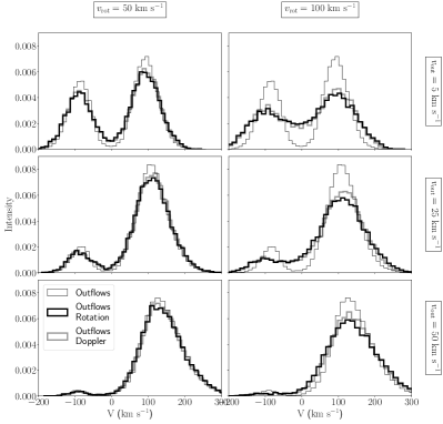
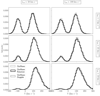
Figure 1: Qualitative trends of changing outflow and rotational velocity viewed perpendicular/paralell to the rotation axis. Here we fix $\tau_{\mathrm{H}}=10^{6}$. The six panels on the left correspond to $\theta=90^{\circ}$ and the panels on the right to $\theta=0^{\circ}$ We vary $v_{\mathrm{rot}}$ increasing from left to right and $v_{\mathrm{out}}$ increasing from top to bottom. The thin black line corresponds to the Ly$\alpha$ line obtained with CLARA without any rotation and the indicated outflow velocity. The thick black line corresponds to CLARA’s results including both outflows and rotation. The thick gray line shows the results of modifying the pure outflow solution (thin black line) by the Doppler shift presented in Equation 4 using the respective $v_{\mathrm{rot}}$ .

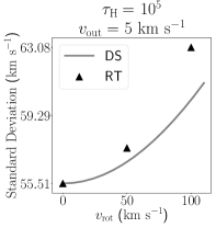
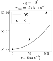
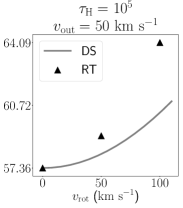
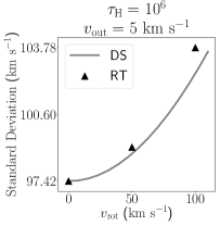
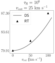
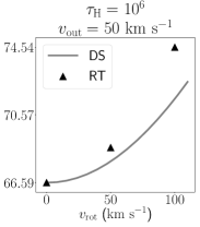
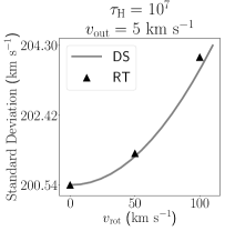
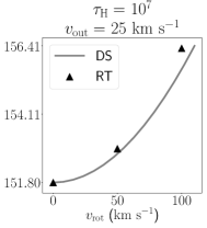
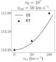
Figure 2: Standard Deviation trends. Results for all the Radiative Transfer simulations (in triangles) compares against the Doppler Shift model (lines). All panels correspond to a viewing angle of $\theta=90^{\circ}$ (perpendicular to the rotation axis). The optical depth increases from top to bottom and the outflow velocity from left to right.

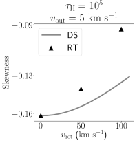
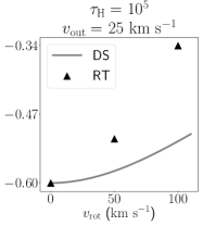
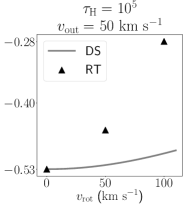
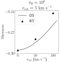
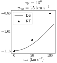
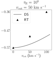
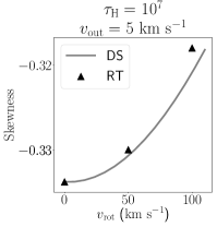
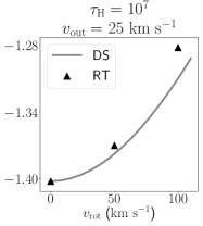
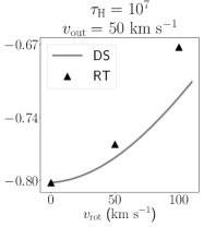
Figure 3: Skewness trends. Results for all the Radiative Transfer simulations (in triangles) compares against the Doppler Shift model (lines). Follows the same layout as Figure 2.

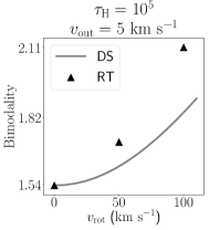
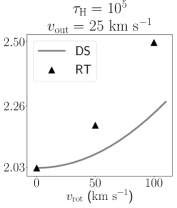
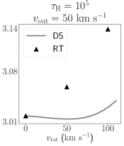
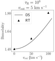
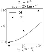
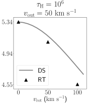
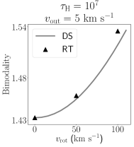
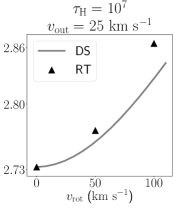
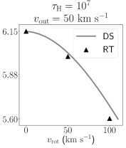
Figure 4: Bimodality trends. Results for all the Radiative Transfer simulations (in triangles) compares against the Doppler Shift model (lines). Follows the same layout as Figure 2.

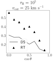
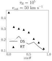
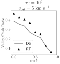
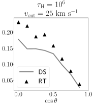
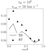
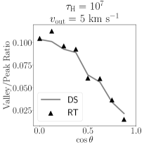
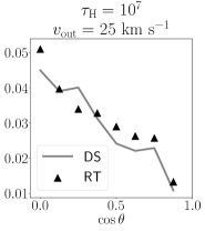
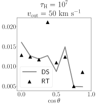
Figure 5: Valley Intensity. We show for each $\tau_{\mathrm{H}}$ the dependency that the viewing angle $\theta$ has on the line’s the valley intensity. $v_{\mathrm{rot}}=100$km s^-1is fixed for all panels.

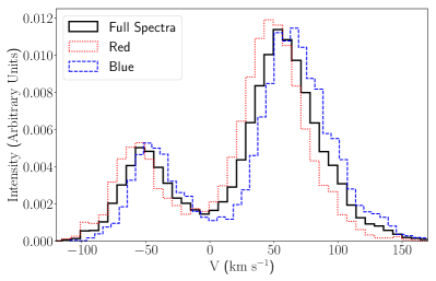
Figure 6: Spectra from receding/approaching sides of a toy model LAE. These results correspond to the RT simulation with $v_{\mathrm{out}}=25$km s^-1, $v_{\mathrm{rot}}=50$km s^-1, $\tau_{\mathrm{H}}=10^{5}$. The spectra were computed for a viewing angle of $\theta=90^{\circ}$. This toy model illustrates to what extent spectra from opposite sides of a galaxy have an imprint of the rotational kinematics.

2 Theoretical Models

We use CLARA (Forero-Romero et al., 2011), a Monte Carlo code that follows the propagation of individual photons through a neutral Hydrogen medium characterized by its temperature, velocity field and global optical depth. The code assumes an homogeneous density throughout the simulated volume. In the current implementation we neglect the influence of dust. Our basic model is an spherical distribution of neutral hydrogen, an approximation commonly used in the literature that explains a wide variety of observational features (Ahn et al., 2003; Verhamme et al., 2006; Dijkstra et al., 2006).

We use a velocity field that captures both outflows and rotation. Outflows are described by a Hubble-like radial velocity profile with the speed increasing linearly with the radial coordinate; this model is fully characterized by $v_{\rm out}$, the radial velocity at the sphere’s surface. Rotation follows a solid body rotation profile fully characterized by $v_{\rm rot}$ the linear velocity at the sphere’s surface.

The total velocity field is the superposition of rotation and outflows. The cartesian components take the following form:

$$v_{x}=\frac{x}{R}v_{\mathrm{out}}-\frac{y}{R}v_{\mathrm{rot}},$$ (1)

$$v_{y}=\frac{y}{R}v_{\mathrm{out}}+\frac{x}{R}v_{\mathrm{rot}},$$ (2)

$$v_{z}=\frac{z}{R}v_{\mathrm{out}},$$ (3)

where $x$, $y$ and $z$ are the cartesian position coordinates with the origin at the sphere’s center, $R$ is the radius of the sphere and the direction of the angular velocity vector is the $z$ axis.

For each run we follow $10^{5}$ individual photons generated from the origin at the Ly$\alpha$ line’s center as they propagate through the volume and finally escape. We store the frequency and propagation direction for each photon at its last scattering.

As input parameters we use $\tau_{\mathrm{H}}=\{10^{5},10^{6},10^{7}\}$, $v_{\mathrm{out}}=\{5,25,50\}\;\mathrm{km\ s}^{-1}$ and $v_{\mathrm{rot}}=\{0,50,100\}\;\mathrm{km\ s}^{-1}$, for a total of $27$ models with all the possible parameter combinations. The values for the outflow velocity are lower than values commonly used in the literature to allow for an interplay between the two kinematic features. This range of parameters also produce emission lines with standard deviation and skewness in the same range to those of high redshift LAES in recent observations (Herenz et al., 2017).

We also define the viewing angle, $\theta$, as the angle between the rotation axis and the line of sight of a potential observer.

Garavito-Camargo et al. (2014) presented an analytical model that accounts for the effects of pure rotation on the Ly$\alpha$ line morphology. The basic assumption of the model is that each differential surface element on the sphere Doppler shifts (DS) the photons that it emits. In this paper we introduce this ansatz by post-processing the results of the outflows simulations without rotation. The frequency of each photon is Doppler shifted as follows

$$x^{\prime}=x+\frac{\vec{v}_{\rm rot}\cdot\hat{k}}{v_{\mathrm{th}}}$$ (4)

where $x^{\prime}$ is the photon’s new adimensional frequency, $x$ is the photon’s frequency after being processed only by the outflow, $v_{\mathrm{rot}}$ is the rotational velocity at the point of escape of the photon, $\hat{k}$ is the photon’s direction of propagation and $v_{\mathrm{th}}$ is the thermal velocity of the sphere. We fix $v_{\mathrm{th}}$ throughout the paper. This factor is a multiplying constant that could be changed without running new Monte-Carlo simulations, as the code works with the adimensional frequency $x$.

This semi-analytic model allows us to produce new Ly$\alpha$ spectra from the outflow-only results and compare them with the full radiative transfer solution including both outflows and rotation.

3 Results

3.1 Qualitative Trends

Figure 1 summarizes the most important trends from the RT simulations. In the left side, the six panels correspond to $\tau=10^{6}$ and a viewing angle of $\theta=90^{\circ}$, that is, perpendicular to the rotation axis of the galaxy. In every panel the thin black line corresponds to the pure outflow solution, i.e. without rotation. From top to bottom we see the effect of increasing the outflow velocity, which is the expected increasing asymmetry towards the red peak.

The thick black line corresponds to the solution that includes both outflows and rotation. Comparing the left and right columns (lower versus higher rotational velocity) we can see two immediate effects. First, the line broadens and second, the intensity at the line’s center increases.

The thick gray line corresponds to the pure outflow solution with the Doppler shift added to model rotation’s influence. At $\tau_{\mathrm{H}}=10^{6}$ the Doppler shift does a good job at capturing the broad morphological features introduced by rotation: the angle dependence, the broadening and the intensity increase at the line’s center.

In the right side of Figure 1 we show the same results as in the left one, but for a viewing angle of $\theta=0^{\circ}$, that is parallel to the rotation axis. In this case we confirm the result presented by Garavito-Camargo et al. (2014), namely that pure rotation introduces a strong dependence with viewing angle, a trend that we find also holds for rotation mixed with outflows.

The quality of the results from the Doppler shift improves for higher $\tau_{\mathrm{H}}$ values. In the Appendix we show the same plots as Figure 1, there it is evident that for $\tau_{\mathrm{H}}=10^{5}$ the results are not as good as they are for $\tau_{\mathrm{H}}=10^{6}$, and that for $\tau_{\mathrm{H}}=10^{7}$ the Doppler shift provides a remarkable good approximation.

3.2 Quantitative Trends

After finding the qualitative influence of the different parameters we move onto a quantitative study. To do this we summarize the line morphology by four different scalars: standard deviation (STD), skewness (SKW), bimodality (BI) and valley/peak ratio. These quantities are defined by the following equations (Kokoska & Zwillinger, 1999):

$$\mathrm{STD}=\sqrt{m_{2}},$$ (5)

$$\mathrm{SKW}=\frac{m_{3}}{m_{2}^{3/2}},$$ (6)

$$\mathrm{BI}=\mathrm{KURTOSIS}-\mathrm{SKW}^{2}=\frac{m_{4}}{m_{2}^{2}}-\frac{m_{3}^{2}}{m_{2}^{3}},$$ (7)

where each $m_{i}$ is the i-th moment about the mean. The STD has velocity units and quantifies the line’s width. The SKW is adimensional and quantifies the peaks’ asymmetry. In the case of a bimodal distribution, $\mathrm{SKW}>0$ means that the blue peak is taller and for $\mathrm{SKW}<0$ the red peak is taller. The BI is adimensional and quantifies whether the line has 1 or 2 peaks: it is always $\geq 1$ (Pearson, 1929) and the closer to 1, the more bimodal is the line (i.e. has 2 similar peaks). We found by visual inspection of our spectra that $\mathrm{BI}=2.5$ marks the transition between two peaks (however imbalanced) and a dominant single peak.

3.2.1 Standard Deviation

Figure 2 summarizes the standard deviation results for all our models. Each panel shows the STD as a function of $v_{\mathrm{rot}}$ . All panels were computed using a viewing angle of $\theta=90^{\circ}$ (perpendicular to the rotation axis), which has the most extreme influence from rotation. The black triangles correspond to the full RT solution and the line to the DS approximation. The optical depth increases from top to bottom and the outflow velocity from left to right. This quantitative plot confirms that the line width increases with rotational velocity and optical depth. These trends are expected; higher rotational velocities can be seen as an addition of different Doppler shifts that smear out the line, while a higher optical depth translates into a larger number of scatterings that increase the probability of a photon to diffuse in frequency resulting in a broader line.

The DS successfully reproduces all trends with the optical depth, rotational velocity and outflow velocity. However, the DS consistently underestimates the STD. The difference between the RT and DS increases with the outflow velocity and the rotational velocity, and decreases with increasing optical depth. In the range of parameter space explore, this difference has as an upper bound of $\sim 7\%$, $3\%$ and $\sim 2\%$ for $\tau_{\mathrm{H}}=10^{5}$, $10^{6}$ and $10^{7}$, respectively.

3.2.2 Skewness

Figure 3 presents the skewness results for all the models together with the DS comparison following the same layout as Figure 2. In all cases the skewness is negative showing that all the lines are unbalanced towards the red side of the spectrum. Skewness increases with rotational velocity and decreases with optical depth; rotation tries to smooth the line diminishing the asymmetries while a higher optical depth reinforces the line asymmetries. The skewness does not have a monotonous trend with outflow velocity because there is a transition between double and single peak line; for low outflow velocities the skewness signals the balance between the two existing peaks while for high outflow velocities it quantifies the asymmetry of the already dominant read peak.

The DS reproduces the main trends, again with an underestimation that decreases at higher optical depths and increases with larger values of the rotational velocity and outflow velocity. In this case the differences between RT and DS have an upper bound of $85\%$, $35\%$ and $5\%$ for $\tau_{\mathrm{H}}=10^{5}$, $10^{6}$ and $10^{7}$, respectively.

3.2.3 Bimodality

Figure 4 shows the results for the bimodality using the same layout as in the two previous Figures. Following the reasoning about the skewness, we observe that increasing the outflow velocity increases the value of bimodality, that is, it transitions to a more pronounced single peak. The trend as a function of the rotational velocity and the optical depth are not monotonous. When the outflow velocity is low ($v_{\mathrm{out}}<50\ \mathrm{km\ s}^{-1}$), an increasing rotational velocity smears the two asymmetrical peaks pushing the line morphology towards a single peaks, making the bimodality statistics increase. On other situations ($v_{\mathrm{out}}=50\ \mathrm{km\ s}^{-1}$ and $\tau_{\mathrm{H}}\geq 10^{6}$) higher rotational velocities the bimodality statistics decreases, which means that it manages to slightly enlarge the already dominant red peak.

The DS reproduces the main trends while underestimating the bimodality statistics. As expected from the previous results the difference between RT and DS decreases at higher optical depths and increases with increasing values of the rotational and outflow velocities. In this case the differences have an upper bound of $4\%$, $2\%$ and $1\%$ for $\tau_{\mathrm{H}}=10^{5}$, $10^{6}$ and $10^{7}$, respectively.

3.2.4 Intensity at line’s center

In Figure 5 we quantify how the intensity at the line’s center (i.e. the valley) changes with the viewing angle, the outflow velocity and the optical depth. These results correspond to a fixed rotational velocity of $v_{\mathrm{rot}}=100\ \mathrm{km\ s}^{-1}$. The triangles correspond to the RT simulations and the line represents the DS results. The valley intensity is expressed as a fraction of the maximum peak intensity in the line, as such the valley/peak ratio is always $<1$. In every panel we see that the valley/peak ratio decreases as the observer moves from a line of sight perpendicular to the rotation axis onto a parallel line of sight. This is a clear demonstration of the viewing angle dependency introduced by rotation.

The valley/peak ratio at $\cos{\theta}=1$ matches results without rotation, this shows that for increasing rotational velocity the valley/peak ratio increases. In turn, for increasing optical depth or outflowing velocity this ratio decreases. Once again, the DS results correctly follow the trends for the full RT simulations. This time the differences have an upper bound of $55\%$, $2\%$ and $1\%$ for $\tau_{\mathrm{H}}=10^{5}$, $10^{6}$ and $10^{7}$, respectively.

4 Discussion

In this section we discuss how the results we have presented can be connected to the interpretation of observational data.

4.1 The semi-analytic model as gaussian smoothing

The effects of the semi-analytic model on the pure outflowing spectra are similar to the expected results from a gaussian smoothing, such smoothing can also be a natural consequence of the intruments used to measure the LAE spectra. As a consequence, natural experimental artifacts could be mistaken as an indication for rotation.

To understand to what extent the effects of rotation can be seen as a simple smoothing, we model the effects of gaussian smoothing with a similar ansatz as the semi-analytic model by changing the frequency of each photon by a Gaussian random variable centered on zero and standard deviation $\sigma_{x}$:

$$x^{\prime}=x+\mathcal{N}(0,\sigma_{x}^{2}).$$ (8)

We find that the results of the semi-analytic model on the total spectra at a given angle $\theta$ can be approximated using $\sigma_{x}=(1/2)\times(v_{\mathrm{rot}}/v_{\mathrm{th}})\times\sin\theta$. This approximation reproduces within a few porcent all quantities measured in Section 3.2 for the semi-analytic model, it only works well for $\tau=10^{6}$ and $\tau=10^{7}$.

This result can be used as an order of magnitude estimate of the mimum espectral resolution required to observe the effects of a rotational velocity of $v_{\mathrm{rot}}$. The Space Telescope Imaging Spectrograph (STIS) on the Hubble Space Telescope (HST) can provide resolutions around 20 km s^-1(Hayes, 2015), which could allow for the detection of rotation features in nearby galaxies with at least $40$ km s^-1and a rotation axis perpendicular to the line of sight. Other instruments such as the Cosmic Origins Spectrograph (COS) have varying resolutions between $20$km s^-1and $200$km s^-1according to the angular size of the source (Orlitová et al., 2018).

4.2 Ly$\alpha$ Kinematic Maps

Current observational facilities have the capability of spatially resolving the extent of a LAE. For instance Prescott et al. (2015) presented observational results of a Doppler shift when taking spectra at two opposite sides of a large ($\approx 80$kpc) LAE. In more recent work Arrigoni Battaia et al. (2018) mapped Ly$\alpha$ emission around a quasar. In this case one could measure the displacement between the peaks in the two different spectra. The interest of this test is that the location of the peaks only depends on the kinematic properties of the sources and does not change by convolution with a gaussian window function due to limited instrumental resolution, as discussed in the previous section.

In Figure 6 we present a toy model ($v_{\mathrm{rot}}$ $=50\ \mathrm{km\ s}^{-1}$, $v_{\mathrm{out}}$ $=25\ \mathrm{km\ s}^{-1}$ and $\tau_{\mathrm{H}}$ $=10^{5}$) for the spectrum of a LAE taken from to different sides of the galaxy. As the LAE is rotating, one side is being redshifted while the other is blueshifted. We see that the full spectrum is a weighted line, in solid black, that is found between these two. We notice that the distance between the maxima of the blue and red spectra is not twice the rotational velocity as it could be naively expected.

In this toy model the distance between the peaks of the receding/approaching spectra is close to $\sim 25\ \mathrm{km\ s}^{-1}$, which is a fourth of the naively expected value of $2v_{\mathrm{rot}}=100\ \mathrm{km\ s}^{-1}$, due to the fact that only a small fraction of the photons are emitted at the extreme of the galaxy having the maximum rotational velocity of $50\ \mathrm{km\ s}^{-1}$. Although it is a good approximation to think the rotating spectra by a sum of Doppler shifts, the peak of the spectra is also weighted by the amount of mass with a given line-of-sight velocity.

Spectrographs like the Multi Unit Spectroscopic Explorer (MUSE) could obtain kinematic information from large samples of LAEs to build velocity maps in Ly$\alpha$. This could be a natural extension of the work reported by Herenz et al. (2016) on the velocity maps of several LARS (Lyman Alpha Reference Sample) galaxies. The interpretation of such data could take into account the insights and trends we have presented in this paper.

5 Conclusions

In this paper we explore, for the first time in the literature, the results of a model for the emergent Ly$\alpha$ line from rotating outflows. We use a semi-analytic model first presented by Garavito-Camargo et al. (2014) to capture the main effects of rotation and confront it against results from Monte-Carlo radiative transfer simulations. The semi-analytic model only takes into account the Doppler shift computed as product of quantities at the surface of last scattering, namely $\vec{v}_{\rm rot}\cdot\hat{k}$, where $\vec{v}_{\rm rot}$ is the velocity due to rotation and $\hat{k}$ is the direction of the photon’s propagation.

To address the first question we posed in the introduction (What is the expected imprint of rotation on a resonant emission line such as the Ly$\alpha$ line?) we find from the full RT simulations that the effects of rotation on the Ly$\alpha$ line morphology are:

• Inducing a dependency on the viewing angle.

• Broadening the line.

• Increasing the intensity at the line’s center.

All these effects can be qualitatively explained by the proposed semi-analytic model. Quantitatively speaking the semi-analytic model provides a satisfactory answer for a neutral Hydrogen optical depth equal or larger than $10^{6}$.

Addressing the second question we posed in the introduction (To what extent is it possible to constrain rotational kinematics from the Ly$\alpha$ emission line?) we show that the most straightforward approach is measuring Ly$\alpha$ spectra from two different regions of a galaxy to detect approaching/receding gas motions (Prescott et al., 2015; Arrigoni Battaia et al., 2018). In that case, we also show that the distances between these two peaks is four times shorter than the naively expected value of $2\times v_{\mathrm{rot}}$. This difference is produced by the different geometric weights at the emitting surface. Here the semi-analytic model also provides the correct quantitative insight.

To summarize, our works shows that the Doppler Shift offers an easy-to-implement approximation to explore such influence into already existing radiative transfer simulations that include outflows, providing a versatile tool to interpret current and future Ly$\alpha$ kinematics maps (e.g Arrigoni Battaia et al., 2018; Erb et al., 2018).

Appendix A Additional figures

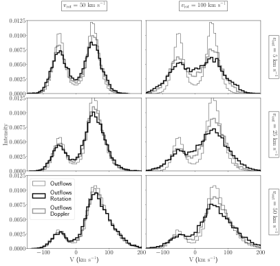
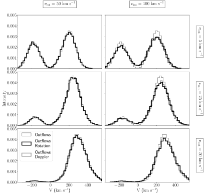
Figure 7: Qualitative trends of changing outflow and rotational velocity. Same layout as Figure 1. On the left: $\tau_{\mathrm{H}}=10^{5}$ and $\theta=90^{\circ}$; on the right: this time $\tau_{\mathrm{H}}=10^{7}$ and $\theta=90^{\circ}$.

References

- Ahn et al. (2003) Ahn S.-H., Lee H.-W., Lee H. M., 2003, MNRAS, 340, 863
- Arrigoni Battaia et al. (2018) Arrigoni Battaia F., Prochaska J. X., Hennawi J. F., Obreja A., Buck T., Cantalupo S., Dutton A. A., Macciò A. V., 2018, MNRAS, 473, 3907
- Cairós & González-Pérez (2017) Cairós L. M., González-Pérez J. N., 2017, A&A, 600, A125
- Cairós et al. (2015) Cairós L. M., Caon N., Weilbacher P. M., 2015, A&A, 577, A21
- Dijkstra et al. (2006) Dijkstra M., Haiman Z., Spaans M., 2006, ApJ, 649, 14
- Erb et al. (2014) Erb D. K., et al., 2014, ApJ, 795, 33
- Erb et al. (2018) Erb D. K., Steidel C. C., Chen Y., 2018, ApJ, 862, L10
- Forero-Romero et al. (2011) Forero-Romero J. E., Yepes G., Gottlöber S., Knollmann S. R., Cuesta A. J., Prada F., 2011, MNRAS, 415, 3666
- Forero-Romero et al. (2018) Forero-Romero J. E., Gronke M., Remolina-Gutiérrez M. C., Garavito-Camargo N., Dijkstra M., 2018, MNRAS, 474, 12