Heavy flavour production in the SACOT-$m_{\rm T}$ scheme

Abstract:

The hadroproduction of heavy-flavoured mesons has recently attracted a growing interest e.g. within the people involved in global analysis of proton and nuclear parton distribution functions, saturation physics, and physics of cosmic rays. In particular, the D- and B-meson measurements of LHCb at forward direction are sensitive to gluon dynamics at small $x$ and are one of the few perturbative small-$x$ probes before the next generation deep-inelastic-scattering experiments. In this talk, we will concentrate on the collinear-factorization approach to inclusive D-meson production and describe a novel implementation — SACOT-$m_{\rm T}$ — of the general-mass variable flavour number scheme (GM-VFNS). In the GM-VFNS framework the cross sections retain the full heavy-quark mass dependence at $p_{\rm T}=0$, but gradually reduce to the ordinary zero-mass results towards asymptotically high $p_{\rm T}$. However, the region of small (but non-zero) $p_{\rm T}$ has been somewhat problematic in the previous implementations of GM-VFNS, leading to divergent cross sections towards $p_{\rm T}\rightarrow 0$, unless the QCD scales are set in a particular way. Here, we provide a solution to this problem. In essence, the idea is to consistently account for the underlying energy-momentum conservation in the presence of a final-state heavy quark-antiquark pair. This automatically leads to a well-behaved GM-VFNS description of the cross sections across all $p_{\rm T}$ without a need to fine tune the QCD scales. The results are compared with the LHCb data and a very good agreement is found. We also compare to fixed-order based calculations and explain why they lead to approximately a factor of two lower D-meson production cross sections than the GM-VFNS approach.

1 Motivation

The potential of D- and B-meson production as a constraint for parton distributions (PDFs) has been recently under active investigation [1, 2, 3]. The heavy-quark mass provides a hard scale offering a possibility to use perturbative QCD for production of heavy-flavoured mesons even down to zero transverse momentum, $P_{\rm T}=0$. While the general-purpose PDFs commonly used for LHC phenomenology are defined in general-mass variable flavour number schemes (GM-VFNS) [4], there are no public GM-VFNS tools for heavy-flavoured meson hadroproduction available. This was the motivation for our study [5] which we summarize here.

2 Heavy-flavour production in fixed flavour-number schemes

In fixed flavour-number schemes (FFNS), the heavy quarks $Q$ are produced in three partonic processes $g+g\rightarrow Q+X,\,q+\overline{q}\rightarrow Q+X,\,q+g\rightarrow Q+X\,$. The rapidity- ($y$) and transverse-momentum ($p_{\rm T}$) differentiated cross section for producing heavy quarks can be written as a convolution of PDFs $f_{i}^{h}(x_{1},\mu^{2}_{\rm fact})$ and partonic cross sections $d\hat{\sigma}$ as

$$\frac{d\sigma(h_{1}+h_{2}\rightarrow{\rm Q}+X)}{dp_{\rm T}dy}= \sum_{ij}\int dx_{1}dx_{2}{f_{i}^{h_{1}}(x_{1},\mu^{2}_{\rm fact})}{\frac{d\hat{\sigma}^{ij\rightarrow{\rm Q}+X}(\tau_{1},\tau_{2},m^{2},\mu^{2}_{\rm ren},\mu^{2}_{\rm fact})}{dp_{\rm T}dy}}{f_{j}^{h_{2}}(x_{2},\mu^{2}_{\rm fact})}\,,$$

where $\tau_{1}\equiv{p_{1}\cdot p_{3}}/{p_{1}\cdot p_{2}}={m_{\rm T}e^{-y}}/({\sqrt{s}x_{2}})$,   $\tau_{2}\equiv{p_{2}\cdot p_{3}}/{p_{1}\cdot p_{2}}={m_{\rm T}e^{y}}/({\sqrt{s}x_{1}})$, and $m_{\rm T}$ represents the transverse mass $m^{2}_{\rm T}={p_{\rm T}^{2}+m^{2}}$. Here $p_{1,2}$ refer to the momenta of the incoming partons, $p_{3}$ is the momentum of the outgoing heavy quark $Q$, and $m$ denotes the heavy-quark mass. The renormalization and factorization scales are denoted by $\mu^{2}_{\rm ren}$ and $\mu^{2}_{\rm fact}$. At high $p_{\rm T}$ the FFNS cross section diverges logarithmically $d\sigma\sim\log(p_{\rm T}^{2}/m^{2})$, so the framework is reliable only at low $p_{\rm T}$.

To convert the parton-level cross sections to hadronic ones, the partonic spectrum is typically folded with a $Q\rightarrow h_{3}$ fragmentation functions (FFs) ${D_{Q\rightarrow h_{3}}(z)}$, fitted to e⁺e^- data. For this we must define a fragmentation variable $z$ which is, however, ambiguous in the presence of massive partons and hadrons. As a working assumption, we shall define $z$ as the fraction of fragmenting heavy-quark’s energy carried by the outgoing hadron $h_{3}$ in the hadronic center-of-mass frame, $z\equiv{E_{\rm hadron}}/{E_{\rm parton}}$. Together with the assumption of collinear fragmentation, this leads to

$$\frac{d\sigma(h_{1}+h_{2}\rightarrow h_{3}+X)}{dP_{\rm T}dY}= \sum_{ij}\int\frac{dz}{z}dx_{1}dx_{2}{f_{i}^{h_{1}}(x_{1},\mu^{2}_{\rm fact})}{\frac{d\hat{\sigma}^{ij\rightarrow{\rm Q}+X}}{dp_{\rm T}dy}}{f_{j}^{h_{2}}(x_{2},\mu^{2}_{\rm fact})}{D_{Q\rightarrow h_{3}}(z)}$$

where the partonic (lower case) and hadronic variables (upper case) are related as

$$p_{\rm T}^{2} =\frac{M^{2}_{\rm T}\cosh^{2}Y-z^{2}m^{2}}{z^{2}}\left(1+\frac{M_{\rm T}^{2}\sinh^{2}Y}{P^{2}_{\rm T}}\right)^{-1}\xrightarrow{P_{\rm T}\rightarrow\infty}\left(\frac{P_{\rm T}}{z}\right)^{2}\,$$

$$y =\sinh^{-1}\left(\frac{M_{\rm T}\sinh Y}{P_{\rm T}}\frac{p_{\rm T}}{m_{\rm T}}\right)\xrightarrow{P_{\rm T}\rightarrow\infty}Y\,$$

where $M_{\rm T}=\sqrt{P_{\rm T}^{2}+M_{h_{3}}^{2}}$ is the hadronic transverse mass. A framework very similar to this has been compared with the LHCb data e.g. in Ref. [6], and the typical situation is that the calculations undershoot the data by a factor of two or so, though within the large scale uncertainties there is still a fair agreement.

3 From FFNS to GM-VFNS heuristically

The GM-VFNS framework can be derived from FFNS by resumming the $\log(p_{\rm T}^{2}/m^{2})$ terms present in the FFNS partonic cross sections. The diagram (a) in Figure 1 shows an NLO diagram in which an incoming gluon splits into a $Q\overline{Q}$ pair giving rise to a collinear logarithm $\sim\log(p_{\rm T}^{2}/m^{2})$. This is just the first term of the whole tower of terms that are in variable flavour number scheme resummed into the heavy-quark PDF $f_{Q}^{h_{1}}$.

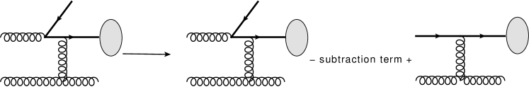
(a)                                         (a)                        (b)                   (c)

Figure 1: A schematic representation of how to deal with the initial-state logarithms.

This resummation can be effectively done by including the heavy-quark initiated contribution (c) and a term (b) that subtracts the overlap between diagrams (a) and (c). We may write the contribution from the $Qg\rightarrow Q+X$ channel as

$$\int\frac{dz}{z}dx_{1}dx_{2}\,{f_{Q}^{h_{1}}(x_{1},\mu^{2}_{\rm fact})}{\frac{d\hat{\sigma}^{Qg\rightarrow{\rm Q}+X}(\tau_{1},\tau_{2})}{dp_{\rm T}dy}}{f_{g}^{h_{2}}(x_{2},\mu^{2}_{\rm fact})}{D_{Q\rightarrow h_{3}}(z)}\,.$$

The compensating subtraction term is obtained from the above expression by swapping the heavy-quark PDF with its perturbative expression to first order in $\alpha_{s}$,

$$f_{Q}(x,\mu^{2}_{\rm fact})=\left(\frac{\alpha_{s}}{2\pi}\right)\log\left(\frac{\mu^{2}_{\rm fact}}{m^{2}}\right)\int_{x}^{1}\frac{\mathrm{d}\ell}{\ell}P_{qg}\left(\frac{x}{\ell}\right)f_{g}(\ell,\mu^{2}_{\rm fact})\,,$$

where $P_{qg}$ is the standard gluon-to-quark splitting function. As is well known [4], the GM-VFNS framework contains an inherent scheme dependence which leaves us with some freedom to choose the exact form of $d\hat{\sigma}^{Qg\rightarrow{\rm Q}+X}(\tau_{1},\tau_{2})$ in the above expressions. In practice, the only requirement is that we must recover the zero-mass expressions at high $p_{\rm T}$,

$${\frac{d\hat{\sigma}^{Qg\rightarrow{\rm Q}+X}(\tau_{1},\tau_{2})}{dp_{\rm T}dy}}\xrightarrow{p_{\rm T}\rightarrow\infty}{\frac{d\hat{\sigma}^{qg\rightarrow{\rm q}+X}(\tau_{1},\tau_{2})}{dp_{\rm T}dy}}\,\,\,\,({\rm q=light\ quark})\,.$$

The simplest option is clearly to use the zero-mass expressions from the outset, ${d\hat{\sigma}^{Qg\rightarrow{\rm Q}+X}(\tau_{1},\tau_{2})}\equiv{d\hat{\sigma}^{qg\rightarrow{\rm q}+X}(\tau_{1},\tau_{2})}$ and also to forget completely about the heavy-quark mass in the kinematics, $\tau_{1,2}\rightarrow{p_{\rm T}e^{\mp y}}/({\sqrt{s}x_{2,1}})$. This defines the so-called SACOT scheme [7]. The problem of this scheme is that since the partonic cross sections behave as ${d\hat{\sigma}^{qg\rightarrow{\rm q}+X}}/d^{3}p\xrightarrow{p_{\rm T}\rightarrow 0}\left(\tau_{1,2}\right)^{-n}$, it leads to infinite (positive or negative) production cross sections towards $P_{\rm T}\rightarrow 0$. This unphysical behaviour can be neatly avoided in what we call here the SACOT-$m_{\rm T}$ scheme [5]: The idea is to retain the $Q\overline{Q}$-pair kinematics also for the $Qg\rightarrow Q+X$ channel, implicitly understanding that the final state must still contain the $\overline{Q}$. With this physical motivation, we define ${d\hat{\sigma}^{Qg\rightarrow{\rm Q}+X}(\tau_{1},\tau_{2})}\equiv{d\hat{\sigma}^{qg\rightarrow{\rm q}+X}(\tau_{1},\tau_{2})}$ taking $\tau_{1,2}={m_{\rm T}e^{\mp y}}/({\sqrt{s}x_{2,1}})$ as in the massive FFNS case. This automatically leads to finite cross sections in the $P_{\rm T}\rightarrow 0$ limit.

There are also collinear logarithms coming from the final-state e.g. when — as in Figure 2 above — an outgoing gluon splits into a $Q\overline{Q}$ pair.

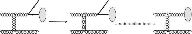
Figure 2: A schematic representation of how to deal with the final-state logarithms.

In this case the $\log(p_{\rm T}^{2}/m^{2})$ terms are resummed into the scale-dependent gluon FFs, $D_{g\rightarrow h_{3}}(z,\mu^{2}_{\rm frag})$. Thus, in GM-VFNS one has also the contribution of the $gg\rightarrow g+X$ channel,

$$\int\frac{dz}{z}dx_{1}dx_{2}\,{f_{g}^{h_{1}}(x_{1},\mu^{2}_{\rm fact})}{\frac{d\hat{\sigma}^{gg\rightarrow g+X}(\tau_{1},\tau_{2})}{dp_{\rm T}dy}}{f_{g}^{h_{2}}(x_{2},\mu^{2}_{\rm fact})}{D_{g\rightarrow h_{3}}(z,\mu^{2}_{\rm frag})}\,.$$

The compensating subtraction term is the same expression, but now with the gluon FF replaced by its perturbative form to first order in $\alpha_{s}$,

$$D_{g\rightarrow h_{3}}(x,\mu^{2}_{\rm frag})=\left(\frac{\alpha_{s}}{2\pi}\right)\log\left(\frac{\mu^{2}_{\rm frag}}{m^{2}}\right)\int_{x}^{1}\frac{\mathrm{d}\ell}{\ell}P_{qg}\left(\frac{x}{\ell}\right)D_{Q\rightarrow h_{3}}(\ell)\,.$$

Consistently with our choice of scheme, also here we use the well-known zero-mass matrix elements for $d\hat{\sigma}^{gg\rightarrow g+X}(\tau_{1},\tau_{2})$ with the massive expressions for $\tau_{1,2}$. The latter accounts for the fact that even if the heavy quarks do not explicitly appear in the $gg\rightarrow g+X$ process, the origins of these contributions are in diagrams where the $Q\overline{Q}$ pair is created. Without going into more details, our final expression in the GM-VFNS is eventually

$$\frac{d\sigma}{dP_{\rm T}dY}=\sum_{ijk}\int\frac{dz}{z}dx_{1}dx_{2}{f_{i}^{h_{1}}(x_{1},\mu^{2}_{\rm fact})}{\frac{d\hat{\sigma}^{ij\rightarrow k}(\tau_{1},\tau_{2},m,\mu^{2}_{\rm ren},\mu^{2}_{\rm fact},\mu^{2}_{\rm frag})}{dp_{\rm T}dy}}{f_{j}^{h_{2}}(x_{2},\mu^{2}_{\rm fact})}{D_{k\rightarrow h_{3}}(z,\mu^{2}_{\rm frag})}\,,$$

where the sum runs over all parton flavours and the fragmentation function is also scale dependent. Towards $p_{\rm T}\rightarrow 0$ the partonic cross sections tend to FFNS ones, but in the $p_{\rm T}\rightarrow\infty$ limit to the zero-mass $\overline{\rm MS}$ expressions. In our numerical implementation, we have taken the light-parton$\rightarrow Q$ expressions up to $\mathcal{O}(\alpha_{s}^{3})$ from the MNR code [8], and all the remaining processes from the INCNLO code [9], up to $\mathcal{O}(\alpha_{s}^{3})$ as well.

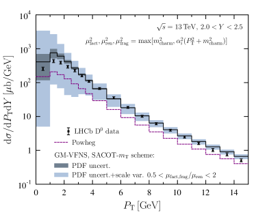
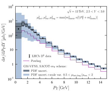
Figure 3: LHCb D⁰ data [10] in proton-proton collisions compared with our GM-VFNS calculation and powheg+pythia framework.

4 Results and discussion

Figure 3 presents a comparison between the LHCb 13 TeV proton-proton data on D⁰ mesons and our GM-VFNS theory calculation. The PDF uncertainty from NNPDF3.1 (pch) [11] is shown in darker colour and the combined scale+PDF uncertainties in light blue. The FFs used are those of Ref. [12]. The agreement is quite excellent though the scale uncertainties are large at small $P_{\rm T}$. We also compare to an approach in which the partonic $c\overline{c}$ events from powheg event generator [13] are showered and hadronized with pythia 8 [14]. Similarly to the FFNS calculations discussed earlier, the powheg+pythia setup tends to underpredict the experimental results by a factor of two. We believe the most significant reason for this is that by starting with $c\overline{c}$ pairs generated by powheg one misses the contributions in which the $c\overline{c}$ pair is created only later in the parton shower. Contributions like these are resummed in GM-VFNS to the scale-dependent FFs and, at high $P_{\rm T}$, e.g. the gluon-to-D contribution is around 50% of the total cross section. In comparison to FFNS, we have also found that these contributions significantly alter the regions where the PDFs are sampled. Therefore, the use of FFNS-based calculations when fitting D-meson data with PDFs poses a potential bias.

References

- [1] O. Zenaiev et al. [PROSA Collaboration], Eur. Phys. J. C 75 (2015) 396.
- [2] R. Gauld and J. Rojo, Phys. Rev. Lett. 118 (2017) 072001.
- [3] A. Kusina, J. P. Lansberg, I. Schienbein and H. S. Shao, Phys. Rev. Lett. 121 (2018) 052004.
- [4] R. S. Thorne and W. K. Tung, arXiv:0809.0714 [hep-ph].
- [5] I. Helenius and H. Paukkunen, JHEP 1805 (2018) 196.
- [6] R. Gauld, J. Rojo, L. Rottoli and J. Talbert, JHEP 1511 (2015) 009.
- [7] B. A. Kniehl, G. Kramer, I. Schienbein and H. Spiesberger, Phys. Rev. D 71 (2005) 014018.
- [8] M. L. Mangano, P. Nason and G. Ridolfi, Nucl. Phys. B 373 (1992) 295.
- [9] F. Aversa, P. Chiappetta, M. Greco and J. P. Guillet, Nucl. Phys. B 327 (1989) 105.
- [10] R. Aaij et al. [LHCb Collaboration], JHEP 1603 (2016) 159.
- [11] R. D. Ball et al. [NNPDF Collaboration], Eur. Phys. J. C 77 (2017) 663.
- [12] T. Kneesch, B. A. Kniehl, G. Kramer and I. Schienbein, Nucl. Phys. B 799 (2008) 34.
- [13] S. Frixione, P. Nason and G. Ridolfi, JHEP 0709 (2007) 126.
- [14] T. Sjöstrand et al., Comput. Phys. Commun. 191 (2015) 159.