Abstract: When estimating the treatment effect in an observational study, we use a semiparametric locally efficient dimension reduction approach to assess both the treatment assignment mechanism and the average responses in both treated and nontreated groups. We then integrate all results through imputation, inverse probability weighting and doubly robust augmentation estimators. Doubly robust estimators are locally efficient while imputation estimators are super-efficient when the response models are correct. To take advantage of both procedures, we introduce a shrinkage estimator to automatically combine the two, which retains the double robustness property while improving on the variance when the response model is correct. We demonstrate the performance of these estimators through simulated experiments and a real dataset concerning the effect of maternal smoking on baby birth weight.

Key Words: Average Treatment Effect, Doubly Robust Estimator, Efficiency, Inverse Probability Weighting, Shrinkage Estimator.

1 Introduction

Dimension reduction is a major methodological issue that must be tackled in modern observational studies where the interest lies in the estimation of the causal effect of a non-randomized treatment. This is due to the increasing availability of health and administrative registers, giving access to high-dimensional pre-treatment information sets which can help identifying causal effects of interest. This paper introduces and studies estimators of average causal effect of a binary treatment using semi-parametric sufficient dimension reduction methods.

Dimension reduction for feasible nonparametric and semiparametric causal inference has only recently been formalized, with most contributions focusing on covariate selection, i.e. methods to pick up which covariates are actual confounders that need to be controlled for, see, e.g., Gruber & van der Laan (2010); de Luna et al. (2011); Farrell (2015); Shortreed & Ertefaie (2017). Dimension reduction must consider nuisance conditional models; the probability of treatment given the covariates (propensity score), and models for the two potential responses (i.e. responses under two possible levels of a binary treatment) given the covariates (de Luna et al., 2011). Sufficient dimension reduction (Li, 1991; Li & Duan, 1991; Cook, 1998; Xia et al., 2002; Xia, 2007; Ma & Zhu, 2012) constitutes an alternative to covariate selection which has the advantage that it can, not only consider covariates in isolation as confounders, but also accomodate linear combinations of the whole covariate set. Such methods have only recently attracted attention in semiparametric causal inference, where Liu et al. (2016) considered sufficient dimension reduction for the estimation of the propensity score only, Luo et al. (2017) considered sufficient dimension reduction for the estimation of the response models only, while Ma et al. (2018) considered classical sufficient dimension in all nuisance models.

In this paper we take a general approach to the estimation of average causal effect. We first use efficient semiparametric sufficient dimension reduction methods (Ma & Zhu, 2013, 2014) in all nuisance models explaining the potential responses and the treatment assignment, and then combine these into classical imputation (IMP) and inverse probability weighting (IPW) estimators. While our semiparametric sufficient dimension reduction modelling is very flexible, nuisance models may still be misspecified and thus a double robust estimator (augmented inverse probability weighting estimator) is also considered which allows for the misspecification of one of the nuisance model. The augmented inverse probability weighting (AIPW) estimator is locally efficient, in the sense that it reaches efficiency at the true nuisance models, while the imputation estimator is super-efficient in the sense that if the true response model is known then this knowledge yields a lower asymptotic efficiency bound than the AIPW estimator may reach (Tan, 2007). We therefore propose a novel estimator shrinking the imputation and AIPW estimators towards each other. The shrinkage estimator is also double robust. It is asymptotically equivalent to the AIPW estimator if the response model is misspecified, and if all nuisance models are correctly specified it shrinks towards the imputation estimator which is more efficient than AIPW in this case. In general, it generates an estimator that has no larger variability than both AIPW and IMP.

2 Model and Dimension Reduction

Let $Y_{T}$ be the treatment response under treatment $T$, where $T=1$ if the treatment of interest is applied and $T=0$ if some alternative treatment, for example, placebo or no treatment is applied. Let ${\bf X}\in{\cal R}^{p}$ be the set of pre-treatment covariates. We observe a random sample $\{{\bf X}_{i},T_{i},Y_{1i}T_{i}+Y_{0i}(1-T_{i})\}$, for $i=1,\dots,n$. In particular, $Y_{ti}$ is observed only for unit $i$ such that $T_{i}=t$, and are therefore called potential responses. Our goal is to estimate the average causal effect of the treatment, here $D=E(Y_{1}-Y_{0})$. We assume $0<\hbox{pr}(T=1\mid Y_{0},Y_{1},{\bf X})=\hbox{pr}(T=1\mid{\bf X})<1$ throughout. This assumption is often called strong ignorability of the treatment assignment, and yields identification of the parameter $D$ under the above sampling scheme (e.g., Rosenbaum & Rubin, 1983).

We now describe flexible dimension reduction structures that will be combined into different semiparametric estimators for $D$. First, the treatment assignment probability, also called propensity score in the literature, can be modelled as

$$\hbox{pr}(T=1\mid{\bf X}={\bf x})=e^{\eta(\boldsymbol{\alpha}^{\rm T}{\bf x})}/\{1+e^{\eta(\boldsymbol{\alpha}^{\rm T}{\bf x})}\},$$ (1)

where $\eta(\cdot)$ is an unknown function, smooth and bounded from both above and below to guarantee the propensity is strictly in $(0,1)$, and $\boldsymbol{\alpha}$ is an unknown index vector or matrix with dimension $p\times d_{\alpha}$, $p>d_{\alpha}$.

Further, we model $Y_{1}$ given ${\bf X}={\bf x}$ using a flexible dimension reduction model

$$Y_{1}=m_{1}(\boldsymbol{\beta}_{1}^{\rm T}{\bf x})+\epsilon_{1}.$$ (2)

where $E(\epsilon_{1}\mid{\bf x})=0$. Similarly, we model $Y_{0}$ given ${\bf X}={\bf x}$ via

$$Y_{0}=m_{0}(\boldsymbol{\beta}_{0}^{\rm T}{\bf x})+\epsilon_{0},$$ (3)

where $E(\epsilon_{0}\mid{\bf x})=0$. Here, $m_{1}(\cdot),m_{0}(\cdot)$ are unknown functions, and $\boldsymbol{\beta}_{1},\boldsymbol{\beta}_{0}$ are unknown index vectors or matrices with dimension $p\times d_{1}$ and $p\times d_{0}$ respectively, for $p>d_{1},p>d_{0}$.

The models (1), (2) and (3) separately describe the probability of receiving treatment and the mean potential responses without imposing any relation between these models. Hence, based on each of the three models, we can estimate the corresponding unknown parameters and unknown functions involved in the models separately using a random sample. We can then combine these estimators in various ways to estimate the treatment effect $D=E(Y_{1}-Y_{0})$.

2.1 Estimation of Response Models

We first consider (2). Because of the ignorability of the treatment assignment assumption, the subset of the sample that are treated indeed form a random sample to fit model (2). Thus, we can directly implement the semiparametric method of Ma & Zhu (2014) for the estimation of both $\boldsymbol{\beta}_{1}$ and $m_{1}(\cdot)$, based on the subset of the data with $T_{i}=1$. For identifiability reason, we adopt the parameterization of Ma & Zhu (2014) and fix the upper $d_{1}\times d_{1}$ submatrix of $\boldsymbol{\beta}_{1}$ as the identity matrix and leave the lower $(p-d_{1})\times d_{1}$ submatrix arbitrary. The locally efficient estimator of $\boldsymbol{\beta}_{1}$ is thus obtained from solving

$$\sum_{i=1}^{n}t_{i}\{y_{1i}-\widehat{m}_{1}(\boldsymbol{\beta}_{1}^{\rm T}{\bf x}_{i},\boldsymbol{\beta}_{1})\}\widehat{\bf m}_{1}^{\prime}(\boldsymbol{\beta}_{1}^{\rm T}{\bf x}_{i},\boldsymbol{\beta}_{1})\otimes\{{\bf x}_{Li}-\widehat{E}({\bf X}_{Li}\mid\boldsymbol{\beta}_{1}^{\rm T}{\bf x}_{i})\}={\bf 0},$$ (4)

where the Nadaraya-Watson kernel estimator is used to obtain $\widehat{E}({\bf X}_{L}\mid\boldsymbol{\beta}_{1}^{\rm T}{\bf x})$ and the local linear estimator is used to obtain $\widehat{m}_{1}(\boldsymbol{\beta}_{1}^{\rm T}{\bf x},\boldsymbol{\beta}_{1})$ and $\widehat{\bf m}_{1}^{\prime}(\boldsymbol{\beta}_{1}^{\rm T}{\bf x},\boldsymbol{\beta}_{1})$, where ${\bf X}_{L}$ represents the subvector of ${\bf X}$ formed by the lower $p-d_{1}$ components. Specifically, in (4),

$$\widehat{E}({\bf X}_{L}\mid\boldsymbol{\beta}_{1}^{\rm T}{\bf x})=\frac{\sum_{i=1}^{n}{\bf x}_{Li}K_{h}(\boldsymbol{\beta}_{1}^{\rm T}{\bf x}_{i}-\boldsymbol{\beta}_{1}^{\rm T}{\bf x})}{\sum_{i=1}^{n}K_{h}(\boldsymbol{\beta}_{1}^{\rm T}{\bf x}_{i}-\boldsymbol{\beta}_{1}^{\rm T}{\bf x})},$$

and $\widehat{m}_{1}(\boldsymbol{\beta}_{1}^{\rm T}{\bf x},\boldsymbol{\beta}_{1})=c_{0},\widehat{\bf m}_{1}^{\prime}(\boldsymbol{\beta}_{1}^{\rm T}{\bf x},\boldsymbol{\beta}_{1})={\bf c}_{1}$ are the solution to

$$\min_{c_{0},{\bf c}_{1}}\sum_{i=1}^{n}t_{i}\{y_{1i}-c_{0}-{\bf c}_{1}^{\rm T}(\boldsymbol{\beta}_{1}^{\rm T}{\bf x}_{i}-\boldsymbol{\beta}_{1}^{\rm T}{\bf x})\}^{2}K_{h}(\boldsymbol{\beta}_{1}^{\rm T}{\bf x}_{i}-\boldsymbol{\beta}_{1}^{\rm T}{\bf x}).$$ (5)

It is easy to verify that the minimizer of (5) has the explicit form

$$\widehat{m}_{1}(\boldsymbol{\beta}_{1}^{\rm T}{\bf x},\boldsymbol{\beta}_{1}) = A_{11}+{\bf A}_{13}^{\rm T}({\bf A}_{14}-{\bf A}_{13}{\bf A}_{13}^{\rm T})^{-1}{\bf A}_{13}A_{11},$$ (6)

$$\widehat{\bf m}_{1}^{\prime}(\boldsymbol{\beta}_{1}^{\rm T}{\bf x},\boldsymbol{\beta}_{1}) = ({\bf A}_{14}-{\bf A}_{13}{\bf A}_{13}^{\rm T})^{-1}({\bf A}_{12}-{\bf A}_{13}A_{11}),$$

where

$$A_{11}=\frac{\sum_{i=1}^{n}t_{i}y_{1i}K_{h}(\boldsymbol{\beta}_{1}^{\rm T}{\bf x}_{i}-\boldsymbol{\beta}_{1}^{\rm T}{\bf x})}{\sum_{i=1}^{n}t_{i}K_{h}(\boldsymbol{\beta}_{1}^{\rm T}{\bf x}_{i}-\boldsymbol{\beta}_{1}^{\rm T}{\bf x})}, {\bf A}_{12}=\frac{\sum_{i=1}^{n}t_{i}y_{1i}(\boldsymbol{\beta}_{1}^{\rm T}{\bf x}_{i}-\boldsymbol{\beta}_{1}^{\rm T}{\bf x})K_{h}(\boldsymbol{\beta}_{1}^{\rm T}{\bf x}_{i}-\boldsymbol{\beta}_{1}^{\rm T}{\bf x})}{\sum_{i=1}^{n}t_{i}K_{h}(\boldsymbol{\beta}_{1}^{\rm T}{\bf x}_{i}-\boldsymbol{\beta}_{1}^{\rm T}{\bf x})},$$

$${\bf A}_{13}=\frac{\sum_{i=1}^{n}t_{i}(\boldsymbol{\beta}_{1}^{\rm T}{\bf x}_{i}-\boldsymbol{\beta}_{1}^{\rm T}{\bf x})K_{h}(\boldsymbol{\beta}_{1}^{\rm T}{\bf x}_{i}-\boldsymbol{\beta}_{1}^{\rm T}{\bf x})}{\sum_{i=1}^{n}t_{i}K_{h}(\boldsymbol{\beta}_{1}^{\rm T}{\bf x}_{i}-\boldsymbol{\beta}_{1}^{\rm T}{\bf x})}, {\bf A}_{14}=\frac{\sum_{i=1}^{n}t_{i}(\boldsymbol{\beta}_{1}^{\rm T}{\bf x}_{i}-\boldsymbol{\beta}_{1}^{\rm T}{\bf x})^{\otimes 2}K_{h}(\boldsymbol{\beta}_{1}^{\rm T}{\bf x}_{i}-\boldsymbol{\beta}_{1}^{\rm T}{\bf x})}{\sum_{i=1}^{n}t_{i}K_{h}(\boldsymbol{\beta}_{1}^{\rm T}{\bf x}_{i}-\boldsymbol{\beta}_{1}^{\rm T}{\bf x})},$$

and ${\bf a}^{\otimes 2}={\bf a}{\bf a}^{\rm T}$ throughout the text. Note that the above description is a typical profiling estimation procedure for $\boldsymbol{\beta}_{1}$. Once we obtain $\widehat{\boldsymbol{\beta}}_{1}$, we then estimate $m_{1}$ using $\widehat{m}_{1}(\widehat{\boldsymbol{\beta}}_{1}^{\rm T}{\bf x},\widehat{\boldsymbol{\beta}}_{1})$ given in (6).

Theorem 1 of Ma & Zhu (2014) established the property of the above estimator. Specifically, the estimator $\widehat{\boldsymbol{\beta}}_{1}$ satisfies

$$\sqrt{n_{1}}\mbox{vecl}(\widehat{\boldsymbol{\beta}}_{1}-\boldsymbol{\beta}_{1})$$

$$= -{\bf B}_{1}n_{1}^{-1/2}\sum_{i=1}^{n}t_{i}\{y_{1i}-m_{1}(\boldsymbol{\beta}_{1}^{\rm T}{\bf x}_{i})\}\mathrm{vec}[{\bf m}_{1}^{\prime}(\boldsymbol{\beta}_{1}^{\rm T}{\bf x}_{i})\otimes\{{\bf x}_{Li}-E({\bf X}_{Li}\mid\boldsymbol{\beta}_{1}^{\rm T}{\bf x}_{i})\}]+o_{p}(1),$$

where $n_{1}=\sum_{i=1}^{n}T_{i}$, $\mbox{vecl}(\boldsymbol{\beta}_{1})$ is the vector formed by the lower $(p-d_{1})\times d_{1}$ submatrix of $\boldsymbol{\beta}_{1}$, and

$${\bf B}_{1} \equiv \left\{E\left(\frac{\partial\mathrm{vec}[T_{i}\{Y_{1i}-m_{1}(\boldsymbol{\beta}_{1}^{\rm T}{\bf X}_{i})\}{\bf m}_{1}^{\prime}(\boldsymbol{\beta}_{1}^{\rm T}{\bf X}_{i})\otimes\{{\bf X}_{Li}-E({\bf X}_{Li}\mid\boldsymbol{\beta}_{1}^{\rm T}{\bf X}_{i})\}]}{\partial\mbox{vecl}(\boldsymbol{\beta}_{1})^{\rm T}}\right)\right\}^{-1}.$$ (8)

Similar analysis can be used to estimate $\boldsymbol{\beta}_{0}$ and $m_{0}$, using the subset of the dataset corresponding to $T_{i}=0$. Then implementing Theorem 1 from Ma & Zhu (2014), the asymptotic behavior of the efficient estimator $\widehat{\boldsymbol{\beta}}_{0}$ is given by

$$\sqrt{n_{0}}\mbox{vecl}(\widehat{\boldsymbol{\beta}}_{0}-\boldsymbol{\beta}_{0})$$

$$= -{\bf B}_{0}n_{0}^{-1/2}\sum_{i=1}^{n}(1-t_{i})\{y_{0i}-m_{0}(\boldsymbol{\beta}_{0}^{\rm T}{\bf x}_{i})\}\mathrm{vec}[{\bf m}_{0}^{\prime}(\boldsymbol{\beta}_{0}^{\rm T}{\bf x}_{i})\otimes\{{\bf x}_{Li}-E({\bf X}_{Li}\mid\boldsymbol{\beta}_{0}^{\rm T}{\bf x}_{i})\}]+o_{p}(1),$$

where $n_{0}=n-n_{1}$, and

$${\bf B}_{0} \equiv \left\{E\left(\frac{\partial\mathrm{vec}[(1-T_{i})\{Y_{0i}-m_{0}(\boldsymbol{\beta}_{0}^{\rm T}{\bf X}_{i})\}{\bf m}_{0}^{\prime}(\boldsymbol{\beta}_{0}^{\rm T}{\bf X}_{i})\otimes\{{\bf X}_{Li}-E({\bf X}_{Li}\mid\boldsymbol{\beta}_{0}^{\rm T}{\bf X}_{i})\}]}{\partial\mbox{vecl}(\boldsymbol{\beta}_{0})^{\rm T}}\right)\right\}^{-1}.$$ (10)

When the mean function models are correct, the meaning of $\boldsymbol{\beta}_{1}$, $\boldsymbol{\beta}_{0}$, $m_{1}$ and $m_{0}$ is easy to understand. When the models are incorrect, as we shall allow in the sequel, we can understand $\boldsymbol{\beta}_{1}$, $\boldsymbol{\beta}_{0}$, $m_{1}$ and $m_{0}$ as quantities that satisfy

$$E[T\{Y_{1}-m_{1}(\boldsymbol{\beta}_{1}^{\rm T}{\bf X},\boldsymbol{\beta}_{1})\}{\bf m}_{1}^{\prime}(\boldsymbol{\beta}_{1}^{\rm T}{\bf X},\boldsymbol{\beta}_{1})\otimes\{{\bf X}_{L}-E({\bf X}_{L}\mid\boldsymbol{\beta}_{1}^{\rm T}{\bf X})\}]={\bf 0},$$

$$E[(1-T)\{Y_{0}-m_{0}(\boldsymbol{\beta}_{0}^{\rm T}{\bf X},\boldsymbol{\beta}_{0})\}{\bf m}_{0}^{\prime}(\boldsymbol{\beta}_{0}^{\rm T}{\bf X},\boldsymbol{\beta}_{0})\otimes\{{\bf X}_{L}-E({\bf X}_{L}\mid\boldsymbol{\beta}_{0}^{\rm T}{\bf X})\}]={\bf 0},$$

where $m_{1}(\boldsymbol{\beta}_{1}^{\rm T}{\bf x})=E(Y_{1}\mid\boldsymbol{\beta}_{1}^{\rm T}{\bf x})\neq E(Y_{1}\mid{\bf x})$, and $m_{0}(\boldsymbol{\beta}_{0}^{\rm T}{\bf x})=E(Y_{0}\mid\boldsymbol{\beta}_{0}^{\rm T}{\bf x})\neq E(Y_{0}\mid{\bf x}).$

2.2 Estimation of Propensity Score Model

The estimation of $\boldsymbol{\alpha},\eta$ was also studied in the literature (Liu et al., 2016; Ma & Zhu, 2013), hence we directly write out the five step algorithm here for completeness of the content and clarity.

Step 1.

Form the Nadaraya-Watson estimator of $E({\bf X}_{i}\mid\boldsymbol{\alpha}^{\rm T}{\bf x}_{i})$ to obtain $\widehat{E}({\bf X}_{i}\mid\boldsymbol{\alpha}^{\rm T}{\bf x}_{i})$.

Step 2.

Solve $\sum_{i=1}^{n}\mbox{vecl}(\{{\bf x}_{i}-\widehat{E}({\bf X}_{i}\mid\boldsymbol{\alpha}^{\rm T}{\bf x}_{i})\}[t_{i}-1+1/\{1+\exp({\bf 1}_{d}^{\rm T}\boldsymbol{\alpha}^{\rm T}{\bf x}_{i})\}]{\bf 1}_{d}^{\rm T})={\bf 0}$ to obtain a consistent initial estimator $\widetilde{\boldsymbol{\alpha}}$.

Step 3.

Obtain the local linear estimators of $\eta({\bf z},\boldsymbol{\alpha})$ and its first derivative $\eta^{\prime}({\bf z},\boldsymbol{\alpha})$ by solving

$$\sum_{i=1}^{n}\left[t_{i}-\frac{\exp\{b_{0}+{\bf b}_{1}^{\rm T}(\boldsymbol{\alpha}^{\rm T}{\bf x}_{i}-{\bf z})\}}{1+\exp\{b_{0}+{\bf b}_{1}^{\rm T}(\boldsymbol{\alpha}^{\rm T}{\bf x}_{i}-{\bf z})\}}\right]K_{h}(\boldsymbol{\alpha}^{\rm T}{\bf x}_{i}-{\bf z}) = 0$$

$$\sum_{i=1}^{n}\left[t_{i}-\frac{\exp\{b_{0}+{\bf b}_{1}^{\rm T}(\boldsymbol{\alpha}^{\rm T}{\bf x}_{i}-{\bf z})\}}{1+\exp\{b_{0}+{\bf b}_{1}^{\rm T}(\boldsymbol{\alpha}^{\rm T}{\bf x}_{i}-{\bf z})\}}\right](\boldsymbol{\alpha}^{\rm T}{\bf x}_{i}-{\bf z})K_{h}(\boldsymbol{\alpha}^{\rm T}{\bf x}_{i}-{\bf z}) = {\bf 0},$$ (11)

for $b_{0},{\bf b}_{1}$ at ${\bf z}=\boldsymbol{\alpha}^{\rm T}{\bf x}_{1},\dots,\boldsymbol{\alpha}^{\rm T}{\bf x}_{n}$. Write the resulting estimator as $\widehat{\eta}(\boldsymbol{\alpha}^{\rm T}{\bf x}_{i},\boldsymbol{\alpha})$ and $\widehat{{\boldsymbol{\eta}}}^{\prime}(\boldsymbol{\alpha}^{\rm T}{\bf x}_{i},\boldsymbol{\alpha})$.

Step 4

Insert $\widehat{\eta}(\cdot,\boldsymbol{\alpha})$, $\widehat{{\boldsymbol{\eta}}}^{\prime}(\cdot,\boldsymbol{\alpha})$ and $\widehat{E}(\cdot)$ into the estimating equation

$$\sum_{i=1}^{n}\{{\bf x}_{Li}-\widehat{E}({\bf X}_{Li}\mid\boldsymbol{\alpha}^{\rm T}{\bf x}_{i})\}\left[t_{i}-\frac{\exp\{\widehat{\eta}(\boldsymbol{\alpha}^{\rm T}{\bf x}_{i})\}}{1+\exp\{\widehat{\eta}(\boldsymbol{\alpha}^{\rm T}{\bf x}_{i})\}}\right]\widehat{\boldsymbol{\eta}}^{\prime}(\boldsymbol{\alpha}^{\rm T}{\bf x}_{i})^{\rm T}={\bf 0}$$

and solve it to obtain the efficient estimator $\widehat{\boldsymbol{\alpha}}$, using starting value $\widetilde{\boldsymbol{\alpha}}$.

Step 5

Repeat Step 3 at $\boldsymbol{\alpha}=\widehat{\boldsymbol{\alpha}}$ to obtain the final estimator of $\eta(\cdot)$.

We will then form $\widehat{\hbox{pr}}(T=1\mid{\bf X}={\bf x})=\exp\{\widehat{\eta}(\widehat{\boldsymbol{\alpha}}^{\rm T}{\bf x})\}/[1+\exp\{\widehat{\eta}(\widehat{\boldsymbol{\alpha}}^{\rm T}{\bf x})\}]$ and use it in the final calculation of the average causal effect. Let us write

$$p_{i}=\frac{\exp\{\eta(\boldsymbol{\alpha}^{\rm T}{\bf x}_{i})\}}{1+\exp\{\eta(\boldsymbol{\alpha}^{\rm T}{\bf x}_{i})\}},P_{i}=\frac{\exp\{\eta(\boldsymbol{\alpha}^{\rm T}{\bf X}_{i})\}}{1+\exp\{\eta(\boldsymbol{\alpha}^{\rm T}{\bf X}_{i})\}},$$

and define

$${\bf B} \equiv \left\{E\left(\frac{\partial}{\partial\mbox{vecl}(\boldsymbol{\alpha})^{\rm T}}\mathrm{vec}\left[\{{\bf X}_{Li}-E({\bf X}_{Li}\mid\boldsymbol{\alpha}^{\rm T}{\bf X}_{i})\}(T_{i}-P_{i}){\boldsymbol{\eta}}^{\prime}(\boldsymbol{\alpha}^{\rm T}{\bf X}_{i})^{\rm T}\right]\right)\right\}^{-1}.$$ (12)

Then using Lemma 2 from Liu et al. (2016), we have

$$\sqrt{n}\mbox{vecl}(\widehat{\boldsymbol{\alpha}}-\boldsymbol{\alpha})=-{\bf B}n^{-1/2}\sum_{i=1}^{n}(t_{i}-p_{i})\mathrm{vec}[\{{\bf x}_{Li}-E({\bf X}_{Li}\mid\boldsymbol{\alpha}^{\rm T}{\bf x}_{i})\}{\boldsymbol{\eta}}^{\prime}(\boldsymbol{\alpha}^{\rm T}{\bf x}_{i})^{\rm T}]+o_{p}(1).$$ (13)

When the propensity score model is correct, the meaning of $\boldsymbol{\alpha}$ and $\eta$ is clear. When the model is incorrect, as we shall allow in the sequel, $\boldsymbol{\alpha}$ and $\eta$ are the quantities that satisfy

$$E[\{{\bf X}_{L}-E({\bf X}_{L}\mid\boldsymbol{\alpha}^{\rm T}{\bf X})\}\left[T-\frac{\exp\{\eta(\boldsymbol{\alpha}^{\rm T}{\bf X})\}}{1+\exp\{\eta(\boldsymbol{\alpha}^{\rm T}{\bf X})\}}\right]{\boldsymbol{\eta}}^{\prime}(\boldsymbol{\alpha}^{\rm T}{\bf X})^{\rm T}]={\bf 0}$$

where $[1+\exp\{\eta(-\boldsymbol{\alpha}^{\rm T}{\bf x})\}]^{-1}=E(T\mid\boldsymbol{\alpha}^{\rm T}{\bf x})\neq E(T\mid{\bf x}).$

3 Average Causal Effect: Estimators and Properties

We are now ready to propose several estimators for estimating the average treatment effect, based on the semiparametric modeling and estimators described in Section 2. These propositions all take advantage of existing methods in missing at random problems, including imputation and weighting, hence they inherit the properties expected. We also introduce a novel shrinkage estimator combining imputation and weighting, with an optimal property. Let $y_{i}=t_{i}y_{1i}+(1-t_{i})y_{0i}$ be the observed response value.

3.1 Imputation Estimators

First we consider estimating the average causal effect using an imputation approach, first proposed in the context of missing data (Rubin, 1978b). The imputation approach we take here is semiparametric in a spirit similar to the nonparametric imputation (Wang et al., 2012). Specifically, we construct

$$\widehat{E}(Y_{1}) = n^{-1}\sum_{i=1}^{n}\left\{t_{i}y_{i}+(1-t_{i})\widehat{m}_{1}(\widehat{\boldsymbol{\beta}}_{1}^{\rm T}{\bf x}_{i})\right\},$$

$$\widehat{E}(Y_{0}) = n^{-1}\sum_{i=1}^{n}\left\{(1-t_{i})y_{i}+t_{i}\widehat{m}_{0}(\widehat{\boldsymbol{\beta}}_{0}^{\rm T}{\bf x}_{i})\right\},$$

and then form the imputation estimator IMP as $\widehat{D}_{\rm IMP}=\widehat{E}(Y_{1})-\widehat{E}(Y_{0})$.

We further consider an alternative imputation estimator which uses the model predicted values while ignoring the observed responses even when they are available. Specifically, we still form $\widehat{D}_{\rm IMP2}\equiv\widehat{E}(Y_{1})-\widehat{E}(Y_{0})$ for the treatment effect, while using

$$\widehat{E}(Y_{1})=n^{-1}\sum_{i=1}^{n}\widehat{m}_{1}(\widehat{\boldsymbol{\beta}}_{1}^{\rm T}{\bf x}_{i}),\ \ \ \widehat{E}(Y_{0})=n^{-1}\sum_{i=1}^{n}\widehat{m}_{0}(\widehat{\boldsymbol{\beta}}_{0}^{\rm T}{\bf x}_{i}),$$

to obtain the imputation estimator IMP2. The latter is sometimes named outcome regression estimator, see for example Tan (2007).

3.2 (Augmented) Inverse Probability Weighting Estimators

Robins et al. (1994) proposed a class of semiparametric estimators based on inverse probability weighted (IPW) estimating equations, borrowing the idea of Horvitz & Thompson (1952) in the survey sampling literature. Later Liu et al. (2016) implemented the IPW estimator with semiparametric modeling to assess the propensity score function. Following this procedure, the IPW estimator consists in constructing

$$\widehat{E}(Y_{1}) = n^{-1}\sum_{i=1}^{n}\frac{t_{i}y_{i}[1+\exp\{\widehat{\eta}(\widehat{\boldsymbol{\alpha}}^{\rm T}{\bf x}_{i})\}]}{{\exp\{\widehat{\eta}(\widehat{\boldsymbol{\alpha}}^{\rm T}{\bf x}_{i})\}}},$$

$$\widehat{E}(Y_{0}) = n^{-1}\sum_{i=1}^{n}(1-t_{i})y_{i}[1+\exp\{\widehat{\eta}(\widehat{\boldsymbol{\alpha}}^{\rm T}{\bf x}_{i})\}],$$

and then form the estimate of the average causal effect $\widehat{D}_{\rm IPW}\equiv\widehat{E}(Y_{1})-\widehat{E}(Y_{0})$.

If at least one of the mean function models, $m_{1}(\cdot)$ and $m_{0}(\cdot)$, is incorrectly specified, the IMP and IMP2 estimators will be inconsistent. Similarly if $\eta(\cdot)$ is incorrectly specified IPW is not consistent. Because of this, we have used more flexible semiparametric dimension reduction models instead of fully parametric models. However, this lowers, but does not completely eliminate, the chance of model misspecification. Thus, protection from either misspecification via the doubly robust estimator (Robins et al., 1994) is still desired. This leads to the augmented inverse probability weighting estimator (AIPW), which has the property of consistency when either the mean models are correctly specified or the propensity score model is correctly specified. The estimate of average causal effect is still $\widehat{D}_{\rm AIPW}\equiv\widehat{E}(Y_{1})-\widehat{E}(Y_{0})$, where now

$$\widehat{E}(Y_{1}) = n^{-1}\sum_{i=1}^{n}\left\{\frac{t_{i}y_{i}[1+\exp\{\widehat{\eta}(\widehat{\boldsymbol{\alpha}}^{\rm T}{\bf x}_{i})\}]}{{\exp\{\widehat{\eta}(\widehat{\boldsymbol{\alpha}}^{\rm T}{\bf x}_{i})\}}}+\left(1-\frac{t_{i}[1+\exp\{\widehat{\eta}(\widehat{\boldsymbol{\alpha}}^{\rm T}{\bf x}_{i})\}]}{\exp\{\widehat{\eta}(\widehat{\boldsymbol{\alpha}}^{\rm T}{\bf x}_{i})\}}\right)\widehat{m}_{1}(\widehat{\boldsymbol{\beta}}_{1}^{\rm T}{\bf x}_{i})\right\}$$

$$\widehat{E}(Y_{0}) = n^{-1}\sum_{i=1}^{n}\left\{(1-t_{i})y_{i}[1+\exp\{\widehat{\eta}(\widehat{\boldsymbol{\alpha}}^{\rm T}{\bf x}_{i})\}]+\left(1-(1-t_{i})[1+\exp\{\widehat{\eta}(\widehat{\boldsymbol{\alpha}}^{\rm T}{\bf x}_{i})\}]\right)\widehat{m}_{0}(\widehat{\boldsymbol{\beta}}_{0}^{\rm T}{\bf x}_{i})\right\}.$$

An improved version of the AIPW estimator was proposed in Robins et al. (1995), which provides extra protection against deteriorated estimation variability. Based on this idea, Tan (2006) later developed a nonparametric likelihood estimator. Adopting this idea in the treatment effect estimation framework, we construct the estimator

$$\widehat{E}(Y_{1}) = n^{-1}\sum_{i=1}^{n}\left\{\frac{t_{i}y_{i}[1+\exp\{\widehat{\eta}(\widehat{\boldsymbol{\alpha}}^{\rm T}{\bf x}_{i})\}]}{{\exp\{\widehat{\eta}(\widehat{\boldsymbol{\alpha}}^{\rm T}{\bf x}_{i})\}}}+\widehat{\gamma}_{1}\left(1-\frac{t_{i}[1+\exp\{\widehat{\eta}(\widehat{\boldsymbol{\alpha}}^{\rm T}{\bf x}_{i})\}]}{\exp\{\widehat{\eta}(\widehat{\boldsymbol{\alpha}}^{\rm T}{\bf x}_{i})\}}\right)\widehat{m}_{1}(\widehat{\boldsymbol{\beta}}_{1}^{\rm T}{\bf x}_{i})\right\}$$

$$\widehat{E}(Y_{0}) = n^{-1}\sum_{i=1}^{n}\left\{(1-t_{i})y_{i}[1+\exp\{\widehat{\eta}(\widehat{\boldsymbol{\alpha}}^{\rm T}{\bf x}_{i})\}]+\widehat{\gamma}_{0}\left(1-(1-t_{i})[1+\exp\{\widehat{\eta}(\widehat{\boldsymbol{\alpha}}^{\rm T}{\bf x}_{i})\}]\right)\widehat{m}_{0}(\widehat{\boldsymbol{\beta}}_{0}^{\rm T}{\bf x}_{i})\right\},$$

and estimate the average causal effect by $\widehat{D}_{\rm IAIPW}\equiv\widehat{E}(Y_{1})-\widehat{E}(Y_{0})$. Here

$$\widehat{\gamma}_{1} = \hbox{cov}\left\{m_{1}(\widehat{\boldsymbol{\beta}}_{1}^{\rm T}{\bf x}_{i})\frac{t_{i}[1+\exp\{\widehat{\eta}(\widehat{\boldsymbol{\alpha}}^{\rm T}{\bf x}_{i})\}]}{{\exp\{\widehat{\eta}(\widehat{\boldsymbol{\alpha}}^{\rm T}{\bf x}_{i})\}}},\left(1-\frac{t_{i}[1+\exp\{\widehat{\eta}(\widehat{\boldsymbol{\alpha}}^{\rm T}{\bf x}_{i})\}]}{\exp\{\widehat{\eta}(\widehat{\boldsymbol{\alpha}}^{\rm T}{\bf x}_{i})\}}\right)\widehat{m}_{1}(\widehat{\boldsymbol{\beta}}_{1}^{\rm T}{\bf x}_{i})\right\}^{-1}$$

$$\times\hbox{cov}\left\{\frac{t_{i}y_{i}[1+\exp\{\widehat{\eta}(\widehat{\boldsymbol{\alpha}}^{\rm T}{\bf x}_{i})\}]}{{\exp\{\widehat{\eta}(\widehat{\boldsymbol{\alpha}}^{\rm T}{\bf x}_{i})\}}},\left(1-\frac{t_{i}[1+\exp\{\widehat{\eta}(\widehat{\boldsymbol{\alpha}}^{\rm T}{\bf x}_{i})\}]}{\exp\{\widehat{\eta}(\widehat{\boldsymbol{\alpha}}^{\rm T}{\bf x}_{i})\}}\right)\widehat{m}_{1}(\widehat{\boldsymbol{\beta}}_{1}^{\rm T}{\bf x}_{i})\right\},$$

$$\widehat{\gamma}_{0} = \hbox{cov}\left\{(1-t_{i})\widehat{m}_{0}(\widehat{\boldsymbol{\beta}}_{0}^{\rm T}{\bf x}_{i})[1+\exp\{\widehat{\eta}(\widehat{\boldsymbol{\alpha}}^{\rm T}{\bf x}_{i})\}],\left(1-(1-t_{i})[1+\exp\{\widehat{\eta}(\widehat{\boldsymbol{\alpha}}^{\rm T}{\bf x}_{i})\}]\right)\widehat{m}_{0}(\widehat{\boldsymbol{\beta}}_{0}^{\rm T}{\bf x}_{i})\right\}^{-1}$$

$$\times\hbox{cov}\left\{(1-t_{i})y_{i}[1+\exp\{\widehat{\eta}(\widehat{\boldsymbol{\alpha}}^{\rm T}{\bf x}_{i})\}],\left(1-(1-t_{i})[1+\exp\{\widehat{\eta}(\widehat{\boldsymbol{\alpha}}^{\rm T}{\bf x}_{i})\}]\right)\widehat{m}_{0}(\widehat{\boldsymbol{\beta}}_{0}^{\rm T}{\bf x}_{i})\right\}.$$

3.3 The Shrinkage Estimator

The ideas of imputation and weighting are quite different and each has its own advantage and drawback. For example, when the treatment mean models $m_{1}(\boldsymbol{\beta}_{1}^{\rm T}{\bf X}),m_{0}(\boldsymbol{\beta}_{0}^{\rm T}{\bf x})$ are correct, regardless if the propensity score model is correct or not, both IMP and AIPW are consistent but it is unclear which estimator is more efficient. However, when the treatment mean models $m_{1}(\boldsymbol{\beta}_{1}^{\rm T}{\bf X}),m_{0}(\boldsymbol{\beta}_{0}^{\rm T}{\bf x})$ are not both correct, AIPW is still consistent as long as the propensity score model is correct, while IMP methods will be inconsistent. Of course, if both the mean models and the propensity models are incorrect, then neither methods will provide consistent estimation. In applications, we typically do not know which scenario we are in, hence it is hard to determine whether IMP methods or AIPW methods are beneficial to use. Because of this situation, in order to take advantage of both methods, we use the idea of shrinkage estimator (Mukherjee & Chatterjee, 2008) to construct a weighted average between IMP and AIPW.

The general observation is that if IMP is consistent, then AIPW is also automatically consistent, but not the other way round. However, it is not generally clear which estimator is more efficient. We construct the following shrinkage estimator: Let $\sqrt{n}(\widehat{D}_{\rm AIPW}-D_{\rm AIPW})\to N(0,v_{\rm AIPW})$ in distribution, $\sqrt{n}(\widehat{D}_{\rm IMP}-D_{\rm IMP})\to N(0,v_{\rm IMP})$ in distribution, and let $\hbox{cov}\{\sqrt{n}(\widehat{D}_{\rm AIPW}-D_{\rm AIPW}),\sqrt{n}(\widehat{D}_{\rm IMP}-D_{\rm IMP})\}\to v_{\rm AI}$. We form

$$w=\frac{(\widehat{D}_{\rm AIPW}-\widehat{D}_{\rm IMP})^{2}+(v_{\rm IMP}-v_{\rm AI})/\sqrt{n}}{(\widehat{D}_{\rm AIPW}-\widehat{D}_{\rm IMP})^{2}+(v_{\rm IMP}+v_{\rm AIPW}-2v_{\rm AI})/\sqrt{n}},$$

and form the shrinkage estimator

$$\widehat{D}=w\widehat{D}_{\rm AIPW}+(1-w)\widehat{D}_{\rm IMP},$$

where we replace $v_{\rm AIPW},v_{\rm IMP},v_{\rm AI}$ with their estimated version. We can see that this construction has the property that when IMP is inconsistent while AIPW is consistent, $w\to 1$ and we essentially obtain AIPW, i.e. the shrinkage estimator is double robust. On the other hand, when both estimators are consistent,

$$w\to\left\{w_{0}\equiv\frac{v_{\rm IMP}-v_{\rm AI}}{v_{\rm IMP}+v_{\rm AIPW}-2v_{\rm AI}}\right\},$$

in probability, which yields the optimal combination of the two estimators in terms of the final estimation variability. Of course when both estimators are inconsistent, the weighted average is still inconsistent.

To construct the shrinkage estimator described above, we derived the asymptotic variances and covariances of the estimators in Section 3.4. Note that one may also choose to shrink IMP2 and AIPW or any of the two versions of the imputation estimator with the improved AIPW in a similar fashion.

3.4 Asymptotic properties of the treatment effect estimators

In this section, we discuss the asymptotic properties of the average treatment effect estimators introduced. These properties are developed under the following conditions:

1. The univariate $m$th order kernel function $K(\cdot)$ is symmetric, Lipschitz continuous on its support $[-1,1]$, which satisfies

   $$\int K(u)du=1,\ \int u^{i}K(u)du=0,1\leq i\leq m-1,\ 0\neq\int u^{m}K(u)du<\infty.$$

2. The bandwidths satisfy $nh^{2m}\to 0$, $nh^{2d}\to\infty$.

3. The probability density functions of $\boldsymbol{\beta}_{1}^{\rm T}{\bf x}$, $\boldsymbol{\beta}_{0}^{\rm T}{\bf x}$ and $\boldsymbol{\alpha}^{\rm T}{\bf x}$, denoted $f\left(\boldsymbol{\beta}^{\rm T}{\bf x}\right)$, $f\left(\boldsymbol{\alpha}^{\rm T}{\bf x}\right)$ and $f\left(\boldsymbol{\alpha}^{\rm T}{\bf x}\right)$ with an abuse of notation, are bounded away from 0 and $\infty$.

Let the true average causal effect be $D=E(Y_{1}-Y_{0})$. Then we have the following results.

Theorem 3.1.

Under the regularity conditions C1-C3, when $n\rightarrow\infty$, the IMP estimator $\widehat{D}_{\rm IMP}$ satisfies $\sqrt{n}(\widehat{D}_{\rm IMP}-D)\overset{d}{\rightarrow}{\rm N}(0,v_{\rm IMP}),$ where combining the results regarding $\widehat{E}(Y_{1})$ and $\widehat{E}(Y_{0})$ in Appendix A.3, we get

$$v_{\rm IMP} = E(\sqrt{n}[\{\widehat{E}(Y_{1})-E(Y_{1})\}-\{\widehat{E}(Y_{0})-E(Y_{0})\}])^{2}$$

$$= E\big{(}\left\{m_{1}(\boldsymbol{\beta}_{1}^{\rm T}{\bf x}_{i})-m_{0}(\boldsymbol{\beta}_{0}^{\rm T}{\bf x}_{i})-E(Y_{1})+E(Y_{0})\right\}$$

$$+E[1+\exp\{-\eta(\boldsymbol{\alpha}^{\rm T}{\bf X}_{i})\}\mid\boldsymbol{\beta}_{1}^{\rm T}{\bf x}_{i}]t_{i}\{y_{1i}-m_{1}(\boldsymbol{\beta}_{1}^{\rm T}{\bf x}_{i})\}$$

$$-E[1+\exp\{\eta(\boldsymbol{\alpha}^{\rm T}{\bf X}_{i})\}\mid\boldsymbol{\beta}_{0}^{\rm T}{\bf x}_{i}](1-t_{i})\{y_{0i}-m_{0}(\boldsymbol{\beta}_{0}^{\rm T}{\bf x}_{i})\}$$

$$-E[(1-P_{i})\mathrm{vec}\{{\bf X}_{Li}{\bf m}_{1}^{\prime}(\boldsymbol{\beta}_{1}^{\rm T}{\bf X}_{i})^{\rm T}\}]^{\rm T}{\bf B}_{1}$$

$$\times t_{i}\{y_{1i}-m_{1}(\boldsymbol{\beta}_{1}^{\rm T}{\bf x}_{i})\}\mathrm{vec}[{\bf m}_{1}^{\prime}(\boldsymbol{\beta}_{1}^{\rm T}{\bf x}_{i})\otimes\{{\bf x}_{Li}-E({\bf X}_{Li}\mid\boldsymbol{\beta}_{1}^{\rm T}{\bf x}_{i})\}]$$

$$+E[P_{i}\mathrm{vec}\{{\bf X}_{Li}{\bf m}_{0}^{\prime}(\boldsymbol{\beta}_{0}^{\rm T}{\bf X}_{i})^{\rm T}\}]^{\rm T}{\bf B}_{0}$$

$$\times(1-t_{i})\{y_{0i}-m_{0}(\boldsymbol{\beta}_{0}^{\rm T}{\bf x}_{i})\}\mathrm{vec}[{\bf m}_{0}^{\prime}(\boldsymbol{\beta}_{0}^{\rm T}{\bf x}_{i})\otimes\{{\bf x}_{Li}-E({\bf X}_{Li}\mid\boldsymbol{\beta}_{0}^{\rm T}{\bf x}_{i})\}]\big{)}^{2},$$

where ${\bf B}_{1}$ and ${\bf B}_{0}$ are defined in (8) and (10), respectively.

Theorem 3.2.

Under the regularity conditions C1-C3, when $n\rightarrow\infty$, the IMP2 estimator $\widehat{D}_{\rm IMP2}$ satisfies $\sqrt{n}(\widehat{D}_{\rm IMP2}-D)\overset{d}{\rightarrow}{\rm N}(0,v_{\rm IMP2}),$ where combining the results regarding $\widehat{E}(Y_{1})$ and $\widehat{E}(Y_{0})$ from Appendix A.4, we get

$$v_{\rm IMP2} = E\big{(}\sqrt{n}[\{\widehat{E}(Y_{1})-E(Y_{1})\}-\{\widehat{E}(Y_{0})-E(Y_{0})\}]\big{)}^{2}$$

$$= E\big{(}\left\{m_{1}(\boldsymbol{\beta}_{1}^{\rm T}{\bf x}_{i})-m_{0}(\boldsymbol{\beta}_{0}^{\rm T}{\bf x}_{i})-E(Y_{1})+E(Y_{0})\right\}$$

$$+E[1+\exp\{-\eta(\boldsymbol{\alpha}^{\rm T}{\bf X}_{i})\}\mid\boldsymbol{\beta}_{1}^{\rm T}{\bf x}_{i}]t_{i}\{y_{1i}-m_{1}(\boldsymbol{\beta}_{1}^{\rm T}{\bf x}_{i})\}$$

$$-E[1+\exp\{\eta(\boldsymbol{\alpha}^{\rm T}{\bf X}_{i})\}\mid\boldsymbol{\beta}_{0}^{\rm T}{\bf x}_{i}](1-t_{i})\{y_{0i}-m_{0}(\boldsymbol{\beta}_{0}^{\rm T}{\bf x}_{i})\}$$

$$-E[\mathrm{vec}\{{\bf X}_{Li}{\bf m}_{1}^{\prime}(\boldsymbol{\beta}_{1}^{\rm T}{\bf X}_{i})^{\rm T}\}]^{\rm T}{\bf B}_{1}t_{i}\{y_{1i}-m_{1}(\boldsymbol{\beta}_{1}^{\rm T}{\bf x}_{i})\}\mathrm{vec}[{\bf m}_{1}^{\prime}(\boldsymbol{\beta}_{1}^{\rm T}{\bf x}_{i})\otimes\{{\bf x}_{Li}-E({\bf X}_{Li}\mid\boldsymbol{\beta}_{1}^{\rm T}{\bf x}_{i})\}]$$

$$+E[\mathrm{vec}\{{\bf X}_{Li}{\bf m}_{0}^{\prime}(\boldsymbol{\beta}_{0}^{\rm T}{\bf X}_{i})^{\rm T}\}]^{\rm T}{\bf B}_{0}$$

$$\times(1-t_{i})\{y_{0i}-m_{0}(\boldsymbol{\beta}_{0}^{\rm T}{\bf x}_{i})\}\mathrm{vec}[{\bf m}_{0}^{\prime}(\boldsymbol{\beta}_{0}^{\rm T}{\bf x}_{i})\otimes\{{\bf x}_{Li}-E({\bf X}_{Li}\mid\boldsymbol{\beta}_{0}^{\rm T}{\bf x}_{i})\}]\big{)}^{2},$$

where ${\bf B}_{1}$ and ${\bf B}_{0}$ are defined in (8) and (10), respectively.

Theorem 3.3.

Under the regularity conditions C1-C3, when $n\rightarrow\infty$, the IPW estimator $\widehat{D}_{\rm IPW}$ satisfies $\sqrt{n}(\widehat{D}_{\rm IPW}-D)\overset{d}{\rightarrow}{\rm N}(0,v_{\rm IPW}),$ where combining the results of $\widehat{E}(Y_{1})$ and $\widehat{E}(Y_{0})$ in Appendix A.1, we get

$$v_{\rm IPW} = E\big{(}\sqrt{n}[\{\widehat{E}(Y_{1})-\widehat{E}(Y_{0})\}-\{E(Y_{1})-E(Y_{0})\}]\big{)}^{2}$$

$$= E\bigg{(}\left\{\frac{t_{i}y_{1i}}{p_{i}}-E(Y_{1})-\frac{(1-t_{i})y_{0i}}{1-p_{i}}+E(Y_{0})\right\}$$

$$+\left(1-\frac{t_{i}}{p_{i}}\right)E\left\{m_{1}(\boldsymbol{\beta}_{1}^{\rm T}{\bf X}_{i})\mid\boldsymbol{\alpha}^{\rm T}{\bf x}_{i}\right\}-\left(\frac{t_{i}-p_{i}}{1-p_{i}}\right)E\left\{m_{0}(\boldsymbol{\beta}_{0}^{\rm T}{\bf X}_{i})\mid\boldsymbol{\alpha}^{\rm T}{\bf x}_{i}\right\}$$

$$+\left(E\left[\frac{m_{1i}(\boldsymbol{\beta}_{1}^{\rm T}{\bf X}_{i})+\exp\{\eta(\boldsymbol{\alpha}^{\rm T}{\bf X}_{i})\}m_{0i}(\boldsymbol{\beta}_{0}^{\rm T}{\bf X}_{i})}{1+\exp\{\eta(\boldsymbol{\alpha}^{\rm T}{\bf X}_{i})\}}\mathrm{vec}\{{\bf X}_{Li}{\boldsymbol{\eta}}^{\prime}(\boldsymbol{\alpha}^{\rm T}{\bf X}_{i})^{\rm T}\}\right]\right)^{\rm T}{\bf B}$$

$$\times(t_{i}-p_{i})\mathrm{vec}[\{{\bf x}_{Li}-E({\bf X}_{Li}\mid\boldsymbol{\alpha}^{\rm T}{\bf x}_{i})\}{\boldsymbol{\eta}}^{\prime}(\boldsymbol{\alpha}^{\rm T}{\bf x}_{i})^{\rm T}]\bigg{)}^{2},$$

where ${\bf B}$ is defined in (12).

Theorem 3.4.

Under the regularity conditions C1-C3, when $n\rightarrow\infty$, the AIPW estimator $\widehat{D}_{\rm AIPW}$ satisfies $\sqrt{n}(\widehat{D}_{\rm AIPW}-D)\overset{d}{\rightarrow}{\rm N}(0,v_{\rm AIPW}),$ where $v_{\rm AIPW}$ derived in Appendix A.2 is

$$v_{\rm AIPW} = E\big{(}\sqrt{n}[\{\widehat{E}(Y_{1})-\widehat{E}(Y_{0})\}-\{E(Y_{1})-E(Y_{0})\}]\big{)}^{2}$$

$$= E\left(\{y_{1i}-m_{1}(\boldsymbol{\beta}_{1}^{\rm T}{\bf x}_{i})\}t_{i}[1+\exp\{-\eta(\boldsymbol{\alpha}^{\rm T}{\bf x}_{i})\}]+m_{1}(\boldsymbol{\beta}_{1}^{\rm T}{\bf x}_{i})-E(Y_{1})\right.$$

$$-{\bf C}_{1}{\bf B}_{1}t_{i}\{y_{1i}-m_{1}(\boldsymbol{\beta}_{1}^{\rm T}{\bf x}_{i})\}\mathrm{vec}[{\bf m}_{1}^{\prime}(\boldsymbol{\beta}_{1}^{\rm T}{\bf x}_{i})\otimes\{{\bf x}_{Li}-E({\bf X}_{Li}\mid\boldsymbol{\beta}_{1}^{\rm T}{\bf x}_{i})\}]$$

$$+{\bf D}_{1}{\bf B}(t_{i}-p_{i})\mathrm{vec}[\{{\bf x}_{Li}-E({\bf X}_{Li}\mid\boldsymbol{\alpha}^{\rm T}{\bf x}_{i})\}{\boldsymbol{\eta}}^{\prime}(\boldsymbol{\alpha}^{\rm T}{\bf x}_{i})^{\rm T}]$$

$$-\{y_{0i}-m_{0}(\boldsymbol{\beta}_{0}^{\rm T}{\bf x}_{i})\}(1-t_{i})[1+\exp\{\eta(\boldsymbol{\alpha}^{\rm T}{\bf x}_{i})\}]-m_{0}(\boldsymbol{\beta}_{0}^{\rm T}{\bf x}_{i})+E(Y_{0})$$

$$+{\bf C}_{0}{\bf B}_{0}(1-t_{i})\{y_{0i}-m_{0}(\boldsymbol{\beta}_{0}^{\rm T}{\bf x}_{i})\}\mathrm{vec}[{\bf m}_{0}^{\prime}(\boldsymbol{\beta}_{0}^{\rm T}{\bf x}_{i})\otimes\{{\bf x}_{Li}-E({\bf X}_{Li}\mid\boldsymbol{\beta}_{0}^{\rm T}{\bf x}_{i})\}]$$

$$\left.+{\bf D}_{0}{\bf B}(t_{i}-p_{i})\mathrm{vec}[\{{\bf x}_{Li}-E({\bf X}_{Li}\mid\boldsymbol{\alpha}^{\rm T}{\bf x}_{i})\}{\boldsymbol{\eta}}^{\prime}(\boldsymbol{\alpha}^{\rm T}{\bf x}_{i})^{\rm T}]\right)^{2},$$

where

$${\bf C}_{1} \equiv E\left\{\frac{\partial m_{1}(\boldsymbol{\beta}_{1}^{\rm T}{\bf X}_{i})}{\partial\mbox{vecl}(\boldsymbol{\beta}_{1})^{\rm T}}(1-T_{i}[1+\exp\{-\eta(\boldsymbol{\alpha}^{\rm T}{\bf X}_{i})\}])\right\},$$

$${\bf D}_{1} \equiv E\left[\{Y_{1i}-m_{1}(\boldsymbol{\beta}_{1}^{\rm T}{\bf X}_{i})\}T_{i}\exp\{-\eta(\boldsymbol{\alpha}^{\rm T}{\bf X}_{i})\}\mathrm{vec}\{{\bf X}_{Li}{\boldsymbol{\eta}}^{\prime}(\boldsymbol{\alpha}^{\rm T}{\bf X}_{i})^{\rm T}\}\right]$$

$${\bf C}_{0} \equiv E\left\{\frac{\partial m_{0}(\boldsymbol{\beta}_{0}^{\rm T}{\bf X}_{i})}{\partial\mbox{vecl}(\boldsymbol{\beta}_{0})^{\rm T}}(1-(1-T_{i})[1+\exp\{\eta(\boldsymbol{\alpha}^{\rm T}{\bf X}_{i})\}])\right\},$$

$${\bf D}_{0} \equiv E\left[\{Y_{0i}-m_{0}(\boldsymbol{\beta}_{0}^{\rm T}{\bf X}_{i})\}(1-T_{i})\exp\{\eta(\boldsymbol{\alpha}^{\rm T}{\bf X}_{i})\}\mathrm{vec}\{{\bf X}_{Li}{\boldsymbol{\eta}}^{\prime}(\boldsymbol{\alpha}^{\rm T}{\bf X}_{i})^{\rm T}\}\right].$$

Note that ${\bf C}_{1}$, ${\bf C}_{0}$, ${\bf D}_{1}$ and ${\bf D}_{0}$ will degenerate to zero if the relevant model is correct. Then

$$v_{\rm AIPW} = E\Big{(}\{y_{1i}-m_{1}(\boldsymbol{\beta}_{1}^{\rm T}{\bf x}_{i})\}t_{i}[1+\exp\{-\eta(\boldsymbol{\alpha}^{\rm T}{\bf x}_{i})\}]+m_{1}(\boldsymbol{\beta}_{1}^{\rm T}{\bf x}_{i})-E(Y_{1})$$

$$- \{y_{0i}-m_{0}(\boldsymbol{\beta}_{0}^{\rm T}{\bf x}_{i})\}(1-t_{i})[1+\exp\{\eta(\boldsymbol{\alpha}^{\rm T}{\bf x}_{i})\}]-m_{0}(\boldsymbol{\beta}_{0}^{\rm T}{\bf x}_{i})+E(Y_{0})\Big{)}^{2}.$$

Noting that $\left(1-t_{i}[1+\exp\{-\eta(\boldsymbol{\alpha}^{\rm T}{\bf x}_{i})\}]\right)m_{1}(\boldsymbol{\beta}_{1}^{\rm T}{\bf x}_{i})$ an $\left(1-(1-t_{i})[1+\exp\{\eta(\boldsymbol{\alpha}^{\rm T}{\bf x}_{i})\}]\right)m_{0}(\boldsymbol{\beta}_{0}^{\rm T}{\bf x}_{i})$ have mean zero, it is straightforward to show that the improved AIPW estimator has the same asymptotic expansion as the AIPW estimator when all three models are correct. Thus, despite their different finite sample performance, the expansion in (3.4) also applies to the improved AIPW estimator. Thus the following result holds.

Theorem 3.5.

Under the regularity conditions C1-C3 and assuming all models are correct, then when $n\rightarrow\infty$, the improved AIPW estimator $\widehat{D}_{\rm IAIPW}$ satisfies $\sqrt{n}(\widehat{D}_{\rm IAIPW}-D)\overset{d}{\rightarrow}{\rm N}(0,v_{\rm AIPW}),$ where $v_{\rm AIPW}$ is here given by (3.4).

Finally, when both estimators $\hat{D}_{IMP}$ and $\hat{D}_{AIPW}$ are consistent, we have

$$\sqrt{n}(\widehat{D}-D) = \sqrt{n}w_{0}(\widehat{D}_{AIPW}-D)+\sqrt{n}(1-w_{0})(\widehat{D}_{IMP}-D)+o_{p}(1),$$

as was noted above.

Theorem 3.6.

Under the regularity conditions C1-C3, when $\widehat{D}_{\rm AIPW}$ and $\widehat{D}_{\rm IMP}$ are consistent and $n\rightarrow\infty$, the shrinkage estimator $\widehat{D}$ satisfies $\sqrt{n}(\widehat{D}-D)\overset{d}{\rightarrow}{\rm N}(0,v_{\rm shrinkage}),$ where $v_{\rm shrinkage}=w_{0}^{2}v_{\rm AIPW}+(1-w_{0})^{2}v_{\rm IMP}+2w_{0}(1-w_{0})v_{\rm AI}$, with

$$v_{\rm AI} = E\left\{\left(\{y_{1i}-m_{1}(\boldsymbol{\beta}_{1}^{\rm T}{\bf x}_{i})\}t_{i}[1+\exp\{-\eta(\boldsymbol{\alpha}^{\rm T}{\bf x}_{i})\}]+m_{1}(\boldsymbol{\beta}_{1}^{\rm T}{\bf x}_{i})-E(Y_{1})\right.\right.$$

$$\left.-\{y_{0i}-m_{0}(\boldsymbol{\beta}_{0}^{\rm T}{\bf x}_{i})\}(1-t_{i})[1+\exp\{\eta(\boldsymbol{\alpha}^{\rm T}{\bf x}_{i})\}]-m_{0}(\boldsymbol{\beta}_{0}^{\rm T}{\bf x}_{i})+E(Y_{0})\right)$$

$$\times\left(t_{i}y_{1i}-(1-t_{i})y_{0i}+(1-t_{i})m_{1}(\boldsymbol{\beta}_{1}^{\rm T}{\bf x}_{i})-t_{i}m_{0}(\boldsymbol{\beta}_{0}^{\rm T}{\bf x}_{i})-E(Y_{1})+E(Y_{0})\right.$$

$$+E[\exp\{-\eta(\boldsymbol{\alpha}^{\rm T}{\bf X}_{i})\}\mid\boldsymbol{\beta}_{1}^{\rm T}{\bf x}_{i}]t_{i}\{y_{1i}-m_{1}(\boldsymbol{\beta}_{1}^{\rm T}{\bf x}_{i})\}$$

$$-E[\exp\{\eta(\boldsymbol{\alpha}^{\rm T}{\bf X}_{i})\}\mid\boldsymbol{\beta}_{0}^{\rm T}{\bf x}_{i}](1-t_{i})\{y_{0i}-m_{0}(\boldsymbol{\beta}_{0}^{\rm T}{\bf x}_{i})\}$$

$$-E[(1-P_{i})\mathrm{vec}\{{\bf X}_{Li}{\bf m}_{1}^{\prime}(\boldsymbol{\beta}_{1}^{\rm T}{\bf X}_{i})^{\rm T}\}]^{\rm T}{\bf B}_{1}t_{i}\{y_{1i}-m_{1}(\boldsymbol{\beta}_{1}^{\rm T}{\bf x}_{i})\}$$

$$\times\mathrm{vec}[{\bf m}_{1}^{\prime}(\boldsymbol{\beta}_{1}^{\rm T}{\bf x}_{i})\otimes\{{\bf x}_{Li}-E({\bf X}_{Li}\mid\boldsymbol{\beta}_{1}^{\rm T}{\bf x}_{i})\}]$$

$$+E[P_{i}\mathrm{vec}\{{\bf X}_{Li}{\bf m}_{0}^{\prime}(\boldsymbol{\beta}_{0}^{\rm T}{\bf X}_{i})^{\rm T}\}]^{\rm T}{\bf B}_{0}(1-t_{i})\{y_{0i}-m_{0}(\boldsymbol{\beta}_{0}^{\rm T}{\bf x}_{i})\}$$

$$\left.\left.\times\mathrm{vec}[{\bf m}_{0}^{\prime}(\boldsymbol{\beta}_{0}^{\rm T}{\bf x}_{i})\otimes\{{\bf x}_{Li}-E({\bf X}_{Li}\mid\boldsymbol{\beta}_{0}^{\rm T}{\bf x}_{i})\}]\right)\right\}.$$

When $\widehat{D}_{IMP}$ is not consistent due to misspecification of at least one of the treatment mean models $m_{1}(\cdot)$ and $m_{0}(\cdot)$, $w\rightarrow 1$, thus $\sqrt{n}(\widehat{D}-D)\overset{d}{\rightarrow}\sqrt{n}(\widehat{D}_{\rm AIPW}-D)$.

4 Simulation Study

We conducted a simulation study to compare the performance of the estimators discussed in Section 3. We used sample size $n=1000$ and covariate dimension $p=6$ with 1000 replicates. Specifically, the covariate vector ${\bf X}=(X_{1},\dots,X_{6})^{\rm T}$ is generated as follows. $X_{1}$ and $X_{2}$ are generated independently from $N(1,1)$ and $N(0,1)$ distribution, respectively. We let $X_{4}=0.015X_{1}+u_{1}$, where $u_{1}$ is uniformly distributed in $(-0.5,0.5)$. Then $X_{3}$ and $X_{5}$ are generated independently from the Bernoulli distribution with success probabilities $0.5+0.05X_{2}$ and $0.4+0.2X_{4}$, respectively. We let $X_{6}=0.04X_{2}+0.15X_{3}+0.05X_{4}+u_{2}$, where $u_{2}\sim N(0,1)$. We set $\boldsymbol{\beta}_{1}=(1,-1,1,-2,-1.5,0.5)^{\rm T}$, $\boldsymbol{\beta}_{0}=(1,1,0,0,0,0)^{\rm T}$ and $\boldsymbol{\alpha}=(-0.27,0.2,-0.15,0.05,0.15,-0.1)^{\rm T}$.

4.1 Study 1

Our first study is designed to study the estimators when the response and propensity score models are correctly specified. We generated the response variables based on $Y_{1}=0.7(\boldsymbol{\beta}_{1}^{\rm T}{\bf x})^{2}+\sin(\boldsymbol{\beta}_{1}^{\rm T}{\bf x})+\epsilon_{1}$ and $Y_{0}=\boldsymbol{\beta}_{0}^{\rm T}{\bf x}+\epsilon_{0}$. Here $\epsilon_{1}$ and $\epsilon_{0}$ are normally distributed with mean zero and variances $0.5$ and $0.2$ respectively. We let further $\eta(\boldsymbol{\alpha}^{\rm T}{\bf x})=\boldsymbol{\alpha}^{\rm T}{\bf x}$. Thus, the treatment indicator $T$ is generated from the logistic model $\hbox{pr}(T=1|{\bf X})={\exp(\boldsymbol{\alpha}^{\rm T}{\bf x})}/\{1+\exp(\boldsymbol{\alpha}^{\rm T}{\bf x})\}.$

We implemented the six estimators described in Section 3. In both the nonparametric estimation of $\eta(\cdot)$ and of the mean functions $m_{1}(\cdot)$ and $m_{0}(\cdot)$, we used local linear regression with Epanechnikov kernel and the bandwidth was chosen to be $c\sigma n^{-1/5}$, where $\sigma^{2}$ is the estimated variances of the corresponding indices, while $c$ is a constant ranging from 0.1 to 3.5. When extrapolation was needed, the local linear fit at the boundary of the support was extrapolated. For comparison, we also computed $\sum_{i=1}^{n}T_{i}Y_{1i}/(\sum_{i=1}^{n}T_{i})-\sum_{i=1}^{n}(1-T_{i})Y_{0i}/(n-\sum_{i=1}^{n}T_{i})$ as the naive sample average estimator.

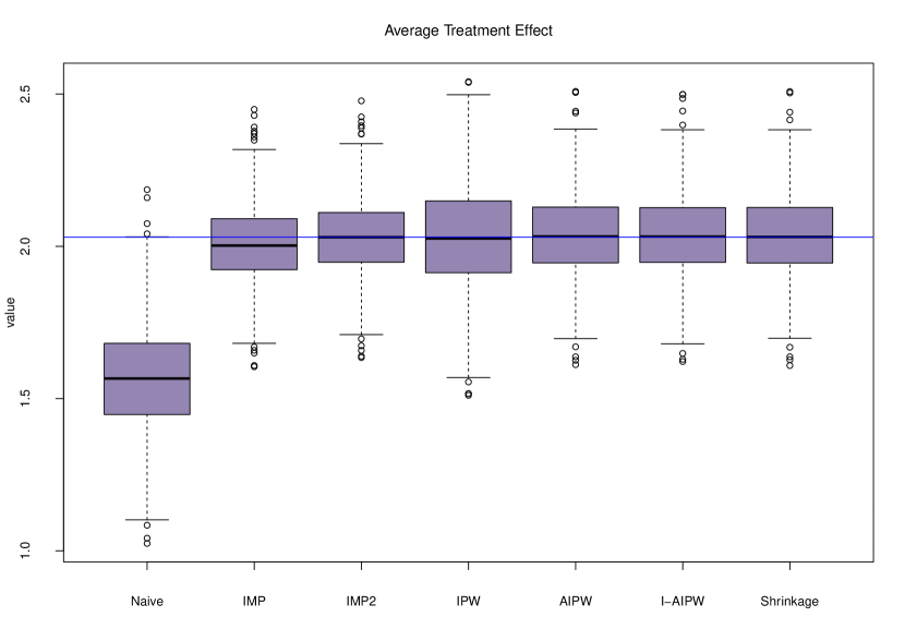
Figure 1: Boxplot of Naive, IMP, IMP2, IPW, AIPW, IAIPW and Shrinkage estimators for Study 1. The blue horizontal line is the true average causal effect, here 2.030.

From the results summarized in Figure 1 and Table 1, we can see that the naive estimator is obviously severely biased. As expected all six methods yield small bias, while IMP2 and IPW provide the smallest and largest variability and mean squared error (MSE) respectively. The estimator shrinking IMP with AIPW improves slightly on the latter with respect to variability and MSE. The estimated standard deviation (based on the asymptotic developments) match fairly well the empirical variability of the estimators.

4.2 Study 2

The second study is designed to compare the performance of the estimators when the mean functions $m_{1}(\cdot)$ and $m_{0}(\cdot)$ are misspecified. We kept the data generation procedure identical to that of Study 1, except that we generated the response variables based on the models $Y_{1}=(\boldsymbol{\beta}_{1}^{\rm T}{\bf x})^{2}+\sin(\boldsymbol{\beta}_{1}^{\rm T}{\bf x})+(\boldsymbol{\gamma}_{1}^{\rm T}{\bf x})^{2}+\epsilon_{1}$ and $Y_{0}=\boldsymbol{\beta}_{0}^{\rm T}{\bf x}+\sin(\boldsymbol{\gamma}_{0}^{\rm T}{\bf x})+\epsilon_{0}$, where $\boldsymbol{\gamma}_{1}=(0,1,1,0,0,0)^{\rm T}$ and $\boldsymbol{\gamma}_{0}=(0,1,-0.75,0,-1,0)^{\rm T}$. Here $\epsilon_{1}$ and $\epsilon_{0}$ are normally distributed with mean zero and variance $0.5$ and $0.2$ respectively. Note that here the mean functions no longer have the single index forms.

When we implemented the six estimators described in Section 3, we still treated $m_{1}(\cdot)$ and $m_{0}(\cdot)$ as function of $\boldsymbol{\beta}_{1}^{\rm T}{\bf x}$ and $\boldsymbol{\beta}_{0}^{\rm T}{\bf x}$ respectively, hence the mean function models we used are misspecified. The same nonparametric estimation procedures as in Study 1 were used in estimating $\eta(\cdot)$, $m_{1}(\cdot)$ and $m_{0}(\cdot)$.

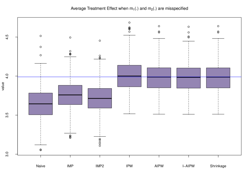
Figure 2: Boxplot of Naive, IMP, IMP2, IPW, AIPW, IAIPW and Shrinkage estimators for Study 2, where $m_{1}(\cdot)$ and $m_{0}(\cdot)$ are misspecified. The blue horizontal line is the true average causal effect, here 3.990.

From the results in Figure 2 and Table 2, we can see that the IMP and IMP2 estimators are biased along with the severely biased naive estimator, while IPW, AIPW, IAIPW and Shrinkage methods yield small bias, even when $m_{1}(\cdot)$ and $m_{0}(\cdot)$ are misspecified as expected. Though IMP is biased, it provides the smallest variability, while IPW yields the largest variability. Here the shrinkage estimator combining IMP and AIPW is able to downweight IMP and inherit lower bias and variability from AIPW. Again estimated standard deviations matches the empirical variability of the estimators.

4.3 Study 3

In a third simulation study, we compare the performance of different estimators when the model of the propensity score function is misspecified. We followed the same data generation procedure as in Section 4.1, but the true function inside the logistic link here is $\eta(\boldsymbol{\alpha}^{\rm T}{\bf x})=(\boldsymbol{\alpha}^{\rm T}{\bf x})+0.45/\{(\boldsymbol{\gamma}^{\rm T}{\bf x})^{2}+0.5\}$, where $\boldsymbol{\gamma}=(1,0.5,-1,0.5,-1,-3)^{\rm T}$. So $\eta(\cdot)$ is no longer a function of a single index. The treatment indicator $T$ is generated from

$$\hbox{pr}(T=1|{\bf X})=\frac{\exp[(\boldsymbol{\alpha}^{\rm T}{\bf x})+0.45/\{(\boldsymbol{\gamma}^{\rm T}{\bf x})^{2}+0.5\}]}{1+\exp[(\boldsymbol{\alpha}^{\rm T}{\bf x})+0.45/\{(\boldsymbol{\gamma}^{\rm T}{\bf x})^{2}+0.5\}]}.$$

In implementing the six estimators described in Section 3, we considered $\eta(\cdot)$ as a function of $\boldsymbol{\alpha}^{\rm T}{\bf x}$ only, thus the propensity score used in estimating the average causal effect was misspecified. Furthermore, we used the same nonparametric approach as in Study 1 and 2 to estimate $m_{1}(\cdot)$, $m_{0}(\cdot)$ and $\eta(\cdot)$.

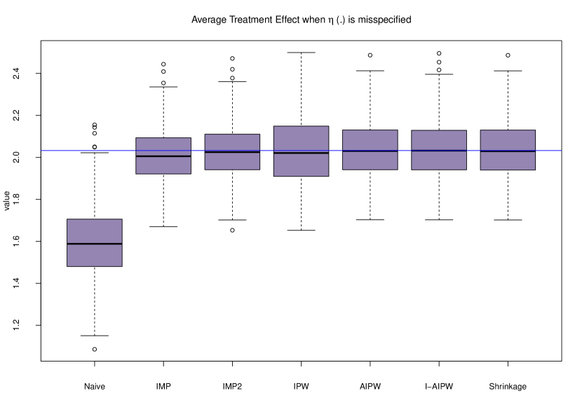
Figure 3: Boxplot of Naive, IMP, IMP2, IPW, AIPW, IAIPW and Shrinkage estimators for Study 3, where $\eta(\cdot)$ is misspecified. The blue horizontal line is the true average causal effect, here 2.033.

The results in Figure 3 and Table 3 show that except for the naive estimator, which is significantly biased, all the six estimators yield small biases. While the small biases of IMP, IMP2, AIPW, IAIPW and the shrinkage estimator are within our expectation, the good performance of IPW is more than what the theory guarantees. Here IMP2 has smallest variability and MSE while IPW performs worst. As in Study 1 both IMP and AIPW are consistent in this design and the shrinkage estimator is again as good as AIPW. By construction, we expect the shrinkage estimator to have lower variability in this situation. This does not show here, probably due to the difficulty in having precise estimates of the asymptotic variances used to compute the shrinkage weight. On the other hand, the variance estimates are sufficiently good to yield satisfactory empirical coverages for the confidence intervals constructed.

4.4 Study 4

In this last study we consider the scenario where all models, $m_{1}(\cdot)$, $m_{0}(\cdot)$ and $\eta(\cdot)$ are misspecified. Here the covariate ${\bf X}$ is generated as in previous studies, the response variables $Y_{1}$ and $Y_{0}$ are generated as in Section 4.2 and the treatment assignment as described in Section 4.3. While implementing the estimators described in Section 3, we still treated $m_{1}(\cdot)$, $m_{0}(\cdot)$ and $\eta(\cdot)$ as functions of $\boldsymbol{\beta}_{1}^{\rm T}{\bf x}$, $\boldsymbol{\beta}_{0}^{\rm T}{\bf x}$ and $\boldsymbol{\alpha}^{\rm T}{\bf x}$ respectively and used the same nonparametric estimation procedure as in earlier sections.

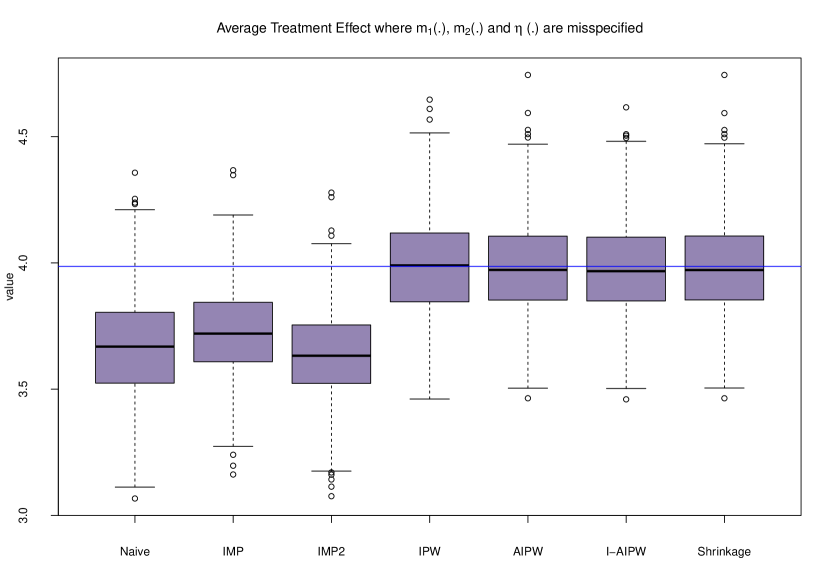
Figure 4: Boxplot of Naive, IMP, IMP2, IPW, AIPW, IAIPW and Shrinkage estimators for Study 4, where $m_{1}(\cdot)$, $m_{0}(\cdot)$ and $\eta(\cdot)$ is misspecified. The blue horizontal line is the true average causal effect, here 3.986.

From Figure 4 and Table 4, we can see that due to misspecification of the mean function models, IMP and IMP2 estimators are biased along with the naive estimator. Like in Study 3, although $\eta(\cdot)$ is misspecified, IPW estimator yields quite small bias. Consequently, AIPW, IAIPW and the Shrinkage estimators are also not significantly influenced by the misspecification of response models and the propensity score model. IMP2 and IMP have lowest variability followed by IAIPW and AIPW, and IPW has the largest variance as in earlier cases. Because IMP has much larger bias than AIPW, the shrinkage estimator mimics AIPW as the theory predicts.

5 Data Analysis

We now apply the methods presented to estimate the average causal effect of maternal smoking during pregnancy on birth weight. The data consist of birth weight (in grams) of 4642 singleton births in Pennsylvania, USA (Almond et al., 2005), for which several covariates are observed: mother’s age, mother’s marital status, an indicator variable for alcohol consumption during pregnancy, an indicator variable of previous birth in which the infant died, mother’s medication, father’s education, number of prenatal care visits, months since last birth, mother’s race and an indicator variable of first born child. The data set also contains the maternal smoking habit during pregnancy and we treat it as our treatment, $T_{i}$ (1=Smoking, 0= Non-Smoking). This dataset was first used by Almond et al. (2005) for studying the economic cost of low brith weights on the society, and was further analyzed in Cattaneo (2010) and Liu et al. (2016). The dataset can be found on http://www.stata-press.com/data/r13/cattaneo2.dta.

Among the 4642 observations, 864 had smoking mothers ($T=1$) and 3778 non-smoking ($T=0$). The naive estimator (without covariate adjustment) yields an effect of -275 grams. We used local linear regression with Epanechnikov kernel in the nonparametric estimation of the propensity score function, $\eta(\cdot)$ and the nonparametric estimation of the mean functions $m_{1}(\cdot)$ and $m_{0}(\cdot)$, where the bandwidth was selected to be $c\sigma n^{-1/5}$, $\sigma^{2}$ is the estimated variance of the corresponding indices and $c$ is a constant. In our analysis, we find that the results are not very sensitive to the value of $c$, for example, when we vary $c$ from from 0.1 to 95, the results hardly change. Applying the six estimators studied in Section 3 yields estimated effects of smoking within the range of -259 to -296 gr. These are displayed in Table 5, together with the estimated standard deviations and the $95$% confidence intervals. IPW stands out with an estimated effect larger than the naive value, and this is due to some observations with propensity scores close to zero, leading to very large weights, thereby also the much larger standard error of IPW. Overall, there is evidence that smoking results in lower birth weight given the assumption that we have observed all confounders.

6 Discussion

We have introduced feasible and robust estimators of average causal effect of a non-randomized treatment. Nuisance models are fitted through semiparametric sufficient dimension reduction methods. Further, parameter estimation in these nuisance models is locally efficient which is important when combined with IPW and IMP estimators. AIPW estimators are efficient and their asymptotic distribution does not depend on the fit of the nuisance parameters as long as the nuisance models are well specified and estimation is consistent (e.g., Farrell, 2015; Belloni et al., 2014). The proposed shrinkage estimator combines AIPW and IMP by improving on efficiency when the nuisance model for the response is correctly specified. When the latter model is misspecified the shrinkage estimator is asymptotically equivalent to AIPW and nothing is lost eventually. Numerical experiments show that the shrinkage estimator is at least as performant as AIPW although no improvement could be observed over AIPW with well specified response models, maybe due to not precise enough weights estimates obtained with the sample size considered. As is the case for IMP, the shrinkage estimator is super-efficient and its asymptotic inference is not expected to be uniform.

Appendix

A.1 Proof of IPW Properties

$$\widehat{E}(Y_{1}) = n^{-1}\sum_{i=1}^{n}\frac{t_{i}y_{i}[1+\exp\{\widehat{\eta}(\widehat{\boldsymbol{\alpha}}^{\rm T}{\bf x}_{i})\}]}{{\exp\{\widehat{\eta}(\widehat{\boldsymbol{\alpha}}^{\rm T}{\bf x}_{i})\}}}$$

$$= n^{-1}\sum_{i=1}^{n}t_{i}y_{1i}\left[\exp\{-\widehat{\eta}(\boldsymbol{\alpha}^{\rm T}{\bf x}_{i})\}+1\right]$$

$$+\left\{\frac{\partial}{\partial\mbox{vecl}(\boldsymbol{\alpha})^{\rm T}}\left(n^{-1}\sum_{i=1}^{n}t_{i}y_{1i}\left[\exp\{-\eta(\boldsymbol{\alpha}^{\rm T}{\bf x}_{i})\}+1\right]\right)+o_{p}(1)\right\}\mbox{vecl}(\widehat{\boldsymbol{\alpha}}-\boldsymbol{\alpha})$$

$$= n^{-1}\sum_{i=1}^{n}t_{i}y_{1i}\left[{\exp\{-\widehat{\eta}(\boldsymbol{\alpha}^{\rm T}{\bf x}_{i})\}}+1\right]$$

$$+\left\{E\left(T_{i}Y_{1i}\mathrm{vec}\left[-\exp\{-\eta(\boldsymbol{\alpha}^{\rm T}{\bf X}_{i})\}{\bf X}_{Li}{\boldsymbol{\eta}}^{\prime}(\boldsymbol{\alpha}^{\rm T}{\bf X}_{i})^{\rm T}\right]\right)\right\}^{\rm T}\mbox{vecl}(\widehat{\boldsymbol{\alpha}}-\boldsymbol{\alpha})+o_{p}(n^{-1/2}).$$

Inserting (13), we have that

$$\left\{E\left(T_{i}Y_{1i}\mathrm{vec}\left[-\exp\{-\eta(\boldsymbol{\alpha}^{\rm T}{\bf X}_{i})\}{\bf X}_{Li}{\boldsymbol{\eta}}^{\prime}(\boldsymbol{\alpha}^{\rm T}{\bf X}_{i})^{\rm T}\right]\right)\right\}^{\rm T}\mbox{vecl}(\widehat{\boldsymbol{\alpha}}-\boldsymbol{\alpha})$$

$$= n^{-1}\sum_{i=1}^{n}\left(E\left[\frac{m_{1i}(\boldsymbol{\beta}_{1}^{\rm T}{\bf X}_{i})}{1+\exp\{\eta(\boldsymbol{\alpha}^{\rm T}{\bf X}_{i})\}}\mathrm{vec}\{{\bf X}_{Li}{\boldsymbol{\eta}}^{\prime}(\boldsymbol{\alpha}^{\rm T}{\bf X}_{i})^{\rm T}\}\right]\right)^{\rm T}{\bf B}$$

$$\times(t_{i}-p_{i})\mathrm{vec}[\{{\bf x}_{Li}-E({\bf X}_{Li}\mid\boldsymbol{\alpha}^{\rm T}{\bf x}_{i})\}{\boldsymbol{\eta}}^{\prime}(\boldsymbol{\alpha}^{\rm T}{\bf x}_{i})^{\rm T}]+o_{p}(n^{-1/2}).$$

In addition, using (A.1) and Condition C2 and C3,

$$n^{-1}\sum_{i=1}^{n}t_{i}y_{1i}\left[{\exp\{-\widehat{\eta}(\boldsymbol{\alpha}^{\rm T}{\bf x}_{i})\}}+1\right]$$

$$= n^{-1}\sum_{j=1}^{n}t_{j}y_{1j}\frac{n^{-1}\sum_{i=1}^{n}K_{h}(\boldsymbol{\alpha}^{\rm T}{\bf x}_{i}-\boldsymbol{\alpha}^{\rm T}{\bf x}_{j})}{n^{-1}\sum_{i=1}^{n}t_{i}K_{h}(\boldsymbol{\alpha}^{\rm T}{\bf x}_{i}-\boldsymbol{\alpha}^{\rm T}{\bf x}_{j})}$$

$$= n^{-1}\sum_{j=1}^{n}t_{j}y_{1j}\left[\frac{f(\boldsymbol{\alpha}^{\rm T}{\bf x}_{j})}{p_{j}f(\boldsymbol{\alpha}^{\rm T}{\bf x}_{j})}+\frac{n^{-1}\sum_{i=1}^{n}K_{h}(\boldsymbol{\alpha}^{\rm T}{\bf x}_{i}-\boldsymbol{\alpha}^{\rm T}{\bf x}_{j})-f(\boldsymbol{\alpha}^{\rm T}{\bf x}_{j})}{p_{j}f(\boldsymbol{\alpha}^{\rm T}{\bf x}_{j})}\right.$$

$$\left.-\frac{f(\boldsymbol{\alpha}^{\rm T}{\bf x}_{j})\{n^{-1}\sum_{i=1}^{n}t_{i}K_{h}(\boldsymbol{\alpha}^{\rm T}{\bf x}_{i}-\boldsymbol{\alpha}^{\rm T}{\bf x}_{j})-p_{j}f(\boldsymbol{\alpha}^{\rm T}{\bf x}_{j})\}}{\{p_{j}f(\boldsymbol{\alpha}^{\rm T}{\bf x}_{j})\}^{2}}\right]+O_{p}\{h^{2m}+(nh^{d})^{-1}\}$$

$$= n^{-1}\sum_{j=1}^{n}\frac{t_{j}y_{1j}}{p_{j}}\left\{1+\frac{n^{-1}\sum_{i=1}^{n}K_{h}(\boldsymbol{\alpha}^{\rm T}{\bf x}_{i}-\boldsymbol{\alpha}^{\rm T}{\bf x}_{j})}{f(\boldsymbol{\alpha}^{\rm T}{\bf x}_{j})}-\frac{n^{-1}\sum_{i=1}^{n}t_{i}K_{h}(\boldsymbol{\alpha}^{\rm T}{\bf x}_{i}-\boldsymbol{\alpha}^{\rm T}{\bf x}_{j})}{p_{j}f(\boldsymbol{\alpha}^{\rm T}{\bf x}_{j})}\right\}+o_{p}(n^{-1/2})$$

$$= n^{-1}\sum_{j=1}^{n}\frac{t_{j}y_{1j}}{p_{j}}+n^{-2}\sum_{j=1}^{n}\sum_{i=1}^{n}\frac{t_{j}y_{1j}(p_{j}-t_{i})K_{h}(\boldsymbol{\alpha}^{\rm T}{\bf x}_{i}-\boldsymbol{\alpha}^{\rm T}{\bf x}_{j})}{p_{j}^{2}f(\boldsymbol{\alpha}^{\rm T}{\bf x}_{j})}+o_{p}(n^{-1/2})$$

$$= n^{-1}\sum_{j=1}^{n}\frac{t_{j}y_{1j}}{p_{j}}+n^{-1}\sum_{j=1}^{n}E\left\{\frac{t_{j}y_{1j}(p_{j}-T_{i})K_{h}(\boldsymbol{\alpha}^{\rm T}{\bf X}_{i}-\boldsymbol{\alpha}^{\rm T}{\bf x}_{j})}{p_{j}^{2}f(\boldsymbol{\alpha}^{\rm T}{\bf x}_{j})}\right\}$$

$$+n^{-1}\sum_{i=1}^{n}E\left\{\frac{T_{j}Y_{1j}(P_{j}-t_{i})K_{h}(\boldsymbol{\alpha}^{\rm T}{\bf x}_{i}-\boldsymbol{\alpha}^{\rm T}{\bf X}_{j})}{P_{j}^{2}f(\boldsymbol{\alpha}^{\rm T}{\bf X}_{j})}\right\}-E\left\{\frac{T_{j}Y_{1j}(P_{j}-T_{i})K_{h}(\boldsymbol{\alpha}^{\rm T}{\bf X}_{i}-\boldsymbol{\alpha}^{\rm T}{\bf X}_{j})}{P_{j}^{2}f(\boldsymbol{\alpha}^{\rm T}{\bf X}_{j})}\right\}$$

$$+o_{p}(n^{-1/2})$$

$$= n^{-1}\sum_{i=1}^{n}\frac{t_{i}y_{1i}}{p_{i}}+n^{-1}\sum_{i=1}^{n}E\left\{m_{1}(\boldsymbol{\beta}_{1}^{\rm T}{\bf X}_{i})\mid\boldsymbol{\alpha}^{\rm T}{\bf x}_{i}\right\}\left(1-\frac{t_{i}}{p_{i}}\right)+o_{p}(n^{-1/2}).$$

We thus obtain

$$\sqrt{n}\widehat{E}(Y_{1}) = n^{-1/2}\sum_{i=1}^{n}\frac{t_{i}y_{1i}}{p_{i}}+n^{-1/2}\sum_{i=1}^{n}E\left\{m_{1}(\boldsymbol{\beta}_{1}^{\rm T}{\bf X}_{i})\mid\boldsymbol{\alpha}^{\rm T}{\bf x}_{i}\right\}\left(1-\frac{t_{i}}{p_{i}}\right)$$ (18)

$$+n^{-1/2}\sum_{i=1}^{n}\left(E\left[\frac{m_{1i}(\boldsymbol{\beta}^{\rm T}{\bf X}_{i})}{1+\exp\{\eta(\boldsymbol{\alpha}^{\rm T}{\bf X}_{i})\}}\mathrm{vec}\{{\bf X}_{Li}{\boldsymbol{\eta}}^{\prime}(\boldsymbol{\alpha}^{\rm T}{\bf X}_{i})^{\rm T}\}\right]\right)^{\rm T}{\bf B}$$

$$\times(t_{i}-p_{i})\mathrm{vec}[\{{\bf x}_{Li}-E({\bf X}_{Li}\mid\boldsymbol{\alpha}^{\rm T}{\bf x}_{i})\}{\boldsymbol{\eta}}^{\prime}(\boldsymbol{\alpha}^{\rm T}{\bf x}_{i})^{\rm T}]+o_{p}(1).$$

Similarly,

$$\widehat{E}(Y_{0}) = n^{-1}\sum_{i=1}^{n}(1-t_{i})y_{i}[1+\exp\{\widehat{\eta}(\widehat{\boldsymbol{\alpha}}^{\rm T}{\bf x}_{i})\}]$$

$$= n^{-1}\sum_{i=1}^{n}(1-t_{i})y_{0i}\left[\exp\{\widehat{\eta}(\boldsymbol{\alpha}^{\rm T}{\bf x}_{i})\}+1\right]$$

$$+\left\{\frac{\partial}{\partial\mbox{vecl}(\boldsymbol{\alpha})^{\rm T}}\left(n^{-1}\sum_{i=1}^{n}(1-t_{i})y_{0i}\left[\exp\{\eta(\boldsymbol{\alpha}^{\rm T}{\bf x}_{i})\}+1\right]\right)+o_{p}(1)\right\}\mbox{vecl}(\widehat{\boldsymbol{\alpha}}-\boldsymbol{\alpha})$$

$$= n^{-1}\sum_{i=1}^{n}(1-t_{i})y_{0i}\left[{\exp\{\widehat{\eta}(\boldsymbol{\alpha}^{\rm T}{\bf x}_{i})\}}+1\right]$$

$$+\left\{E\left((1-T_{i})Y_{0i}\mathrm{vec}\left[\exp\{\eta(\boldsymbol{\alpha}^{\rm T}{\bf X}_{i})\}{\bf X}_{Li}{\boldsymbol{\eta}}^{\prime}(\boldsymbol{\alpha}^{\rm T}{\bf X}_{i})^{\rm T}\right]\right)\right\}^{\rm T}\mbox{vecl}(\widehat{\boldsymbol{\alpha}}-\boldsymbol{\alpha})+o_{p}(n^{-1/2}).$$

We further have that

$$\left\{E\left((1-T_{i})Y_{0i}\mathrm{vec}\left[\exp\{\eta(\boldsymbol{\alpha}^{\rm T}{\bf X}_{i})\}{\bf X}_{Li}{\boldsymbol{\eta}}^{\prime}(\boldsymbol{\alpha}^{\rm T}{\bf X}_{i})^{\rm T}\right]\right)\right\}^{\rm T}\mbox{vecl}(\widehat{\boldsymbol{\alpha}}-\boldsymbol{\alpha})$$

$$= -n^{-1}\sum_{i=1}^{n}\left(E\left[\frac{m_{0i}(\boldsymbol{\beta}_{0}^{\rm T}{\bf X}_{i})\exp\{\eta(\boldsymbol{\alpha}^{\rm T}{\bf X}_{i})\}}{1+\exp\{\eta(\boldsymbol{\alpha}^{\rm T}{\bf X}_{i})\}}\mathrm{vec}\{{\bf X}_{Li}{\boldsymbol{\eta}}^{\prime}(\boldsymbol{\alpha}^{\rm T}{\bf X}_{i})^{\rm T}\}\right]\right)^{\rm T}{\bf B}$$

$$\times(t_{i}-p_{i})\mathrm{vec}[\{{\bf x}_{Li}-E({\bf X}_{Li}\mid\boldsymbol{\alpha}^{\rm T}{\bf x}_{i})\}{\boldsymbol{\eta}}^{\prime}(\boldsymbol{\alpha}^{\rm T}{\bf x}_{i})^{\rm T}]+o_{p}(n^{-1/2}).$$

In addition, using (A.1) and Conditon C2 and C3,

$$n^{-1}\sum_{i=1}^{n}(1-t_{i})y_{0i}\left[{\exp\{\widehat{\eta}(\boldsymbol{\alpha}^{\rm T}{\bf x}_{i})\}}+1\right]$$

$$= n^{-1}\sum_{j=1}^{n}(1-t_{j})y_{0j}\frac{n^{-1}\sum_{i=1}^{n}K_{h}(\boldsymbol{\alpha}^{\rm T}{\bf x}_{i}-\boldsymbol{\alpha}^{\rm T}{\bf x}_{j})}{n^{-1}\sum_{i=1}^{n}(1-t_{i})K_{h}(\boldsymbol{\alpha}^{\rm T}{\bf x}_{i}-\boldsymbol{\alpha}^{\rm T}{\bf x}_{j})}$$

$$= n^{-1}\sum_{j=1}^{n}(1-t_{j})y_{0j}\left[\frac{f(\boldsymbol{\alpha}^{\rm T}{\bf x}_{j})}{(1-p_{j})f(\boldsymbol{\alpha}^{\rm T}{\bf x}_{j})}+\frac{n^{-1}\sum_{i=1}^{n}K_{h}(\boldsymbol{\alpha}^{\rm T}{\bf x}_{i}-\boldsymbol{\alpha}^{\rm T}{\bf x}_{j})-f(\boldsymbol{\alpha}^{\rm T}{\bf x}_{j})}{(1-p_{j})f(\boldsymbol{\alpha}^{\rm T}{\bf x}_{j})}\right.$$

$$\left.-\frac{f(\boldsymbol{\alpha}^{\rm T}{\bf x}_{j})\{n^{-1}\sum_{i=1}^{n}(1-t_{i})K_{h}(\boldsymbol{\alpha}^{\rm T}{\bf x}_{i}-\boldsymbol{\alpha}^{\rm T}{\bf x}_{j})-(1-p_{j})f(\boldsymbol{\alpha}^{\rm T}{\bf x}_{j})\}}{\{(1-p_{j})f(\boldsymbol{\alpha}^{\rm T}{\bf x}_{j})\}^{2}}\right]+O_{p}\{h^{2m}+(nh)^{-1}\}$$

$$= n^{-1}\sum_{j=1}^{n}\frac{(1-t_{j})y_{0j}}{1-p_{j}}\left\{1+\frac{n^{-1}\sum_{i=1}^{n}K_{h}(\boldsymbol{\alpha}^{\rm T}{\bf x}_{i}-\boldsymbol{\alpha}^{\rm T}{\bf x}_{j})}{f(\boldsymbol{\alpha}^{\rm T}{\bf x}_{j})}-\frac{n^{-1}\sum_{i=1}^{n}(1-t_{i})K_{h}(\boldsymbol{\alpha}^{\rm T}{\bf x}_{i}-\boldsymbol{\alpha}^{\rm T}{\bf x}_{j})}{(1-p_{j})f(\boldsymbol{\alpha}^{\rm T}{\bf x}_{j})}\right\}$$

$$+o_{p}(n^{-1/2})$$

$$= n^{-1}\sum_{j=1}^{n}\frac{(1-t_{j})y_{0j}}{1-p_{j}}-n^{-2}\sum_{j=1}^{n}\sum_{i=1}^{n}\frac{(1-t_{j})y_{0j}(p_{j}-t_{i})K_{h}(\boldsymbol{\alpha}^{\rm T}{\bf x}_{i}-\boldsymbol{\alpha}^{\rm T}{\bf x}_{j})}{(1-p_{j})^{2}f(\boldsymbol{\alpha}^{\rm T}{\bf x}_{j})}+o_{p}(n^{-1/2})$$

$$= n^{-1}\sum_{j=1}^{n}\frac{(1-t_{j})y_{0j}}{1-p_{j}}-n^{-1}\sum_{j=1}^{n}E\left\{\frac{(1-t_{j})y_{0j}(p_{j}-T_{i})K_{h}(\boldsymbol{\alpha}^{\rm T}{\bf X}_{i}-\boldsymbol{\alpha}^{\rm T}{\bf x}_{j})}{(1-p_{j})^{2}f(\boldsymbol{\alpha}^{\rm T}{\bf x}_{j})}\right\}$$

$$-n^{-1}\sum_{i=1}^{n}E\left\{\frac{(1-T_{j})Y_{0j}(P_{j}-t_{i})K_{h}(\boldsymbol{\alpha}^{\rm T}{\bf x}_{i}-\boldsymbol{\alpha}^{\rm T}{\bf X}_{j})}{(1-P_{j})^{2}f(\boldsymbol{\alpha}^{\rm T}{\bf X}_{j})}\right\}$$

$$+E\left\{\frac{(1-T_{j})Y_{0j}(P_{j}-T_{i})K_{h}(\boldsymbol{\alpha}^{\rm T}{\bf X}_{i}-\boldsymbol{\alpha}^{\rm T}{\bf X}_{j})}{(1-P_{j})^{2}f(\boldsymbol{\alpha}^{\rm T}{\bf X}_{j})}\right\}+o_{p}(n^{-1/2})$$

$$= n^{-1}\sum_{i=1}^{n}\frac{(1-t_{i})y_{0i}}{1-p_{i}}+n^{-1}\sum_{i=1}^{n}E\left\{m_{0}(\boldsymbol{\beta}_{0}^{\rm T}{\bf X}_{i})\mid\boldsymbol{\alpha}^{\rm T}{\bf x}_{i}\right\}\left(\frac{t_{i}-p_{i}}{1-p_{i}}\right)+o_{p}(n^{-1/2}).$$

We thus obtain

$$\sqrt{n}\widehat{E}(Y_{0}) = n^{-1/2}\sum_{i=1}^{n}\frac{(1-t_{i})y_{0i}}{1-p_{i}}+n^{-1/2}\sum_{i=1}^{n}E\left\{m_{0}(\boldsymbol{\beta}_{0}^{\rm T}{\bf X}_{i})\mid\boldsymbol{\alpha}^{\rm T}{\bf x}_{i}\right\}\left(\frac{t_{i}-p_{i}}{1-p_{i}}\right)$$ (19)

$$-n^{-1/2}\sum_{i=1}^{n}\left(E\left[\frac{m_{0i}(\boldsymbol{\beta}_{0}^{\rm T}{\bf X}_{i})\exp\{\eta(\boldsymbol{\alpha}^{\rm T}{\bf X}_{i})\}}{1+\exp\{\eta(\boldsymbol{\alpha}^{\rm T}{\bf X}_{i})\}}\mathrm{vec}\{{\bf X}_{Li}{\boldsymbol{\eta}}^{\prime}(\boldsymbol{\alpha}^{\rm T}{\bf X}_{i})^{\rm T}\}\right]\right)^{\rm T}{\bf B}$$

$$\times(t_{i}-p_{i})\mathrm{vec}[\{{\bf x}_{Li}-E({\bf X}_{Li}\mid\boldsymbol{\alpha}^{\rm T}{\bf x}_{i})\}{\boldsymbol{\eta}}^{\prime}(\boldsymbol{\alpha}^{\rm T}{\bf x}_{i})^{\rm T}]+o_{p}(1).$$

Combining the results of $\widehat{E}(Y_{1})$ and $\widehat{E}(Y_{0})$, we get

$$\sqrt{n}[\{\widehat{E}(Y_{1})-\widehat{E}(Y_{0})\}-\{E(Y_{1})-E(Y_{0})\}]$$

$$= n^{-1/2}\sum_{i=1}^{n}\left\{\frac{t_{i}y_{1i}}{p_{i}}-E(Y_{1})-\frac{(1-t_{i})y_{0i}}{1-p_{i}}+E(Y_{0})\right\}$$

$$+n^{-1/2}\sum_{i=1}^{n}\left(1-\frac{t_{i}}{p_{i}}\right)E\left\{m_{1}(\boldsymbol{\beta}_{1}^{\rm T}{\bf X}_{i})\mid\boldsymbol{\alpha}^{\rm T}{\bf x}_{i}\right\}-n^{-1/2}\sum_{i=1}^{n}\left(\frac{t_{i}-p_{i}}{1-p_{i}}\right)E\left\{m_{0}(\boldsymbol{\beta}_{0}^{\rm T}{\bf X}_{i})\mid\boldsymbol{\alpha}^{\rm T}{\bf x}_{i}\right\}$$

$$+n^{-1/2}\sum_{i=1}^{n}\left(E\left[\frac{m_{1i}(\boldsymbol{\beta}_{1}^{\rm T}{\bf X}_{i})+\exp\{\eta(\boldsymbol{\alpha}^{\rm T}{\bf X}_{i})\}m_{0i}(\boldsymbol{\beta}_{0}^{\rm T}{\bf X}_{i})}{1+\exp\{\eta(\boldsymbol{\alpha}^{\rm T}{\bf X}_{i})\}}\mathrm{vec}\{{\bf X}_{Li}{\boldsymbol{\eta}}^{\prime}(\boldsymbol{\alpha}^{\rm T}{\bf X}_{i})^{\rm T}\}\right]\right)^{\rm T}{\bf B}$$

$$\times(t_{i}-p_{i})\mathrm{vec}[\{{\bf x}_{Li}-E({\bf X}_{Li}\mid\boldsymbol{\alpha}^{\rm T}{\bf x}_{i})\}{\boldsymbol{\eta}}^{\prime}(\boldsymbol{\alpha}^{\rm T}{\bf x}_{i})^{\rm T}]+o_{p}(1).$$

∎

A.2 Proof of Properties of AIPW

$$\sqrt{n}\{\widehat{E}(Y_{1})-E(Y_{1})\}$$

$$= n^{-1/2}\sum_{i=1}^{n}\left\{t_{i}y_{i}[1+\exp\{-\widehat{\eta}(\widehat{\boldsymbol{\alpha}}^{\rm T}{\bf x}_{i})\}]-E(Y_{1})+\left(1-t_{i}[1+\exp\{-\widehat{\eta}(\widehat{\boldsymbol{\alpha}}^{\rm T}{\bf x}_{i})\}]\right)\widehat{m}_{1}(\widehat{\boldsymbol{\beta}}_{1}^{\rm T}{\bf x}_{i})\right\}$$

$$= n^{-1/2}\sum_{i=1}^{n}\left\{t_{i}y_{1i}[1+\exp\{-\widehat{\eta}(\boldsymbol{\alpha}^{\rm T}{\bf x}_{i})\}]-E(Y_{1})+\left(1-t_{i}[1+\exp\{-\widehat{\eta}(\boldsymbol{\alpha}^{\rm T}{\bf x}_{i})\}]\right)\widehat{m}_{1}(\widehat{\boldsymbol{\beta}}_{1}^{\rm T}{\bf x}_{i})\right\}$$

$$+\left[n^{-1}\sum_{i=1}^{n}t_{i}\{y_{1i}-\widehat{m}_{1}(\widehat{\boldsymbol{\beta}}_{1}^{\rm T}{\bf x}_{i})\}\frac{\partial\exp\{-\widehat{\eta}(\boldsymbol{\alpha}^{\rm T}{\bf x}_{i})\}}{\partial\mbox{vecl}(\boldsymbol{\alpha})^{\rm T}}+o_{p}(1)\right]\sqrt{n}\mbox{vecl}(\widehat{\boldsymbol{\alpha}}-\boldsymbol{\alpha})$$

$$= n^{-1/2}\sum_{i=1}^{n}\left(\{y_{1i}-\widehat{m}_{1}(\widehat{\boldsymbol{\beta}}_{1}^{\rm T}{\bf x}_{i})\}t_{i}[1+\exp\{-\widehat{\eta}(\boldsymbol{\alpha}^{\rm T}{\bf x}_{i})\}]+\widehat{m}_{1}(\widehat{\boldsymbol{\beta}}_{1}^{\rm T}{\bf x}_{i})-E(Y_{1})\right)$$

$$-E\left[\{Y_{1i}-m_{1}(\boldsymbol{\beta}_{1}^{\rm T}{\bf X}_{i})\}T_{i}\exp\{-\eta(\boldsymbol{\alpha}^{\rm T}{\bf X}_{i})\}\mathrm{vec}\{{\bf X}_{Li}{\boldsymbol{\eta}}^{\prime}(\boldsymbol{\alpha}^{\rm T}{\bf X}_{i})^{\rm T}\}\right]\sqrt{n}\mbox{vecl}(\widehat{\boldsymbol{\alpha}}-\boldsymbol{\alpha})+o_{p}(1)$$

$$= n^{-1/2}\sum_{i=1}^{n}\left(\{y_{1i}-\widehat{m}_{1}(\boldsymbol{\beta}_{1}^{\rm T}{\bf x}_{i})\}t_{i}[1+\exp\{-\widehat{\eta}(\boldsymbol{\alpha}^{\rm T}{\bf x}_{i})\}]+\widehat{m}_{1}(\boldsymbol{\beta}_{1}^{\rm T}{\bf x}_{i})-E(Y_{1})\right)$$

$$+\left[E\left\{\frac{\partial m_{1}(\boldsymbol{\beta}_{1}^{\rm T}{\bf X}_{i})}{\partial\mbox{vecl}(\boldsymbol{\beta}_{1})^{\rm T}}(1-T_{i}[1+\exp\{-\eta(\boldsymbol{\alpha}^{\rm T}{\bf X}_{i})\}])\right\}+o_{p}(1)\right]\sqrt{n}\mbox{vecl}(\widehat{\boldsymbol{\beta}}_{1}-\boldsymbol{\beta}_{1})$$

$$-{\bf D}_{1}\sqrt{n}\mbox{vecl}(\widehat{\boldsymbol{\alpha}}-\boldsymbol{\alpha})+o_{p}(1)$$

$$= n^{-1/2}\sum_{i=1}^{n}\left(\{y_{1i}-\widehat{m}_{1}(\boldsymbol{\beta}_{1}^{\rm T}{\bf x}_{i})\}\left(t_{i}[1+\exp\{-\widehat{\eta}(\boldsymbol{\alpha}^{\rm T}{\bf x}_{i})\}]-1\right)+y_{1i}-E(Y_{1})\right)$$

$$+{\bf C}_{1}\sqrt{n}\mbox{vecl}(\widehat{\boldsymbol{\beta}}_{1}-\boldsymbol{\beta}_{1})-{\bf D}_{1}\sqrt{n}\mbox{vecl}(\widehat{\boldsymbol{\alpha}}-\boldsymbol{\alpha})+o_{p}(1)$$

$$= n^{-1/2}\sum_{i=1}^{n}\left\{\{y_{1i}-m_{1}(\boldsymbol{\beta}_{1}^{\rm T}{\bf x}_{i})\}\left(t_{i}[1+\exp\{-\eta(\boldsymbol{\alpha}^{\rm T}{\bf x}_{i})\}]-1\right)+y_{1i}-E(Y_{1})\right\}$$

$$-{\bf C}_{1}{\bf B}_{1}n^{-1/2}\sum_{i=1}^{n}t_{i}\{y_{1i}-m_{1}(\boldsymbol{\beta}_{1}^{\rm T}{\bf x}_{i})\}\mathrm{vec}[{\bf m}_{1}^{\prime}(\boldsymbol{\beta}_{1}^{\rm T}{\bf x}_{i})\otimes\{{\bf x}_{Li}-E({\bf X}_{Li}\mid\boldsymbol{\beta}_{1}^{\rm T}{\bf x}_{i})\}]$$

$$+{\bf D}_{1}{\bf B}n^{-1/2}\sum_{i=1}^{n}(t_{i}-p_{i})\mathrm{vec}[\{{\bf x}_{Li}-E({\bf X}_{Li}\mid\boldsymbol{\alpha}^{\rm T}{\bf x}_{i})\}{\boldsymbol{\eta}}^{\prime}(\boldsymbol{\alpha}^{\rm T}{\bf x}_{i})^{\rm T}]+o_{p}(1)$$

$$= n^{-1/2}\sum_{i=1}^{n}\left(\{y_{1i}-m_{1}(\boldsymbol{\beta}_{1}^{\rm T}{\bf x}_{i})\}t_{i}[1+\exp\{-\eta(\boldsymbol{\alpha}^{\rm T}{\bf x}_{i})\}]+m_{1}(\boldsymbol{\beta}_{1}^{\rm T}{\bf x}_{i})-E(Y_{1})\right.$$

$$-{\bf C}_{1}{\bf B}_{1}t_{i}\{y_{1i}-m_{1}(\boldsymbol{\beta}_{1}^{\rm T}{\bf x}_{i})\}\mathrm{vec}[{\bf m}_{1}^{\prime}(\boldsymbol{\beta}_{1}^{\rm T}{\bf x}_{i})\otimes\{{\bf x}_{Li}-E({\bf X}_{Li}\mid\boldsymbol{\beta}_{1}^{\rm T}{\bf x}_{i})\}]$$

$$\left.+{\bf D}_{1}{\bf B}(t_{i}-p_{i})\mathrm{vec}[\{{\bf x}_{Li}-E({\bf X}_{Li}\mid\boldsymbol{\alpha}^{\rm T}{\bf x}_{i})\}{\boldsymbol{\eta}}^{\prime}(\boldsymbol{\alpha}^{\rm T}{\bf x}_{i})^{\rm T}]\right)+o_{p}(1).$$

Similarly,

$$\sqrt{n}\{\widehat{E}(Y_{0})-E(Y_{0})\}$$

$$= n^{-1/2}\sum_{i=1}^{n}\left\{(1-t_{i})y_{i}[1+\exp\{\widehat{\eta}(\widehat{\boldsymbol{\alpha}}^{\rm T}{\bf x}_{i})\}]-E(Y_{0})+\left(1-(1-t_{i})[1+\exp\{\widehat{\eta}(\widehat{\boldsymbol{\alpha}}^{\rm T}{\bf x}_{i})\}]\right)\widehat{m}_{0}(\widehat{\boldsymbol{\beta}}_{0}^{\rm T}{\bf x}_{i})\right\}$$

$$= n^{-1/2}\sum_{i=1}^{n}\left\{(1-t_{i})y_{0i}[1+\exp\{\widehat{\eta}(\boldsymbol{\alpha}^{\rm T}{\bf x}_{i})\}]-E(Y_{0})+\left(1-(1-t_{i})[1+\exp\{\widehat{\eta}(\boldsymbol{\alpha}^{\rm T}{\bf x}_{i})\}]\right)\widehat{m}_{0}(\widehat{\boldsymbol{\beta}}_{0}^{\rm T}{\bf x}_{i})\right\}$$

$$+\left[n^{-1}\sum_{i=1}^{n}(1-t_{i})\{y_{0i}-\widehat{m}_{0}(\widehat{\boldsymbol{\beta}}_{0}^{\rm T}{\bf x}_{i})\}\frac{\partial\exp\{\widehat{\eta}(\boldsymbol{\alpha}^{\rm T}{\bf x}_{i})\}}{\partial\mbox{vecl}(\boldsymbol{\alpha})^{\rm T}}+o_{p}(1)\right]\sqrt{n}\mbox{vecl}(\widehat{\boldsymbol{\alpha}}-\boldsymbol{\alpha})$$

$$= n^{-1/2}\sum_{i=1}^{n}\left(\{y_{0i}-\widehat{m}_{0}(\widehat{\boldsymbol{\beta}}_{0}^{\rm T}{\bf x}_{i})\}(1-t_{i})[1+\exp\{\widehat{\eta}(\boldsymbol{\alpha}^{\rm T}{\bf x}_{i})\}]+\widehat{m}_{0}(\widehat{\boldsymbol{\beta}}_{0}^{\rm T}{\bf x}_{i})-E(Y_{0})\right)$$

$$+E\left[\{Y_{0i}-m_{0}(\boldsymbol{\beta}_{0}^{\rm T}{\bf X}_{i})\}(1-T_{i})\exp\{\eta(\boldsymbol{\alpha}^{\rm T}{\bf X}_{i})\}\mathrm{vec}\{{\bf X}_{Li}{\boldsymbol{\eta}}^{\prime}(\boldsymbol{\alpha}^{\rm T}{\bf X}_{i})^{\rm T}\}\right]\sqrt{n}\mbox{vecl}(\widehat{\boldsymbol{\alpha}}-\boldsymbol{\alpha})+o_{p}(1)$$

$$= n^{-1/2}\sum_{i=1}^{n}\left(\{y_{0i}-\widehat{m}_{0}(\boldsymbol{\beta}_{0}^{\rm T}{\bf x}_{i})\}(1-t_{i})[1+\exp\{\widehat{\eta}(\boldsymbol{\alpha}^{\rm T}{\bf x}_{i})\}]+\widehat{m}_{0}(\boldsymbol{\beta}_{0}^{\rm T}{\bf x}_{i})-E(Y_{0})\right)$$

$$+\left[E\left\{\frac{\partial m_{0}(\boldsymbol{\beta}_{0}^{\rm T}{\bf X}_{i})}{\partial\mbox{vecl}(\boldsymbol{\beta}_{0})^{\rm T}}(1-(1-T_{i})[1+\exp\{\eta(\boldsymbol{\alpha}^{\rm T}{\bf X}_{i})\}])\right\}+o_{p}(1)\right]\sqrt{n}\mbox{vecl}(\widehat{\boldsymbol{\beta}}_{1}-\boldsymbol{\beta}_{1})$$

$$+{\bf D}_{0}\sqrt{n}\mbox{vecl}(\widehat{\boldsymbol{\alpha}}-\boldsymbol{\alpha})+o_{p}(1)$$

$$= n^{-1/2}\sum_{i=1}^{n}\left(\{y_{0i}-\widehat{m}_{0}(\boldsymbol{\beta}_{0}^{\rm T}{\bf x}_{i})\}\left((1-t_{i})[1+\exp\{\widehat{\eta}(\boldsymbol{\alpha}^{\rm T}{\bf x}_{i})\}]-1\right)+y_{0i}-E(Y_{0})\right)$$

$$+{\bf C}_{0}\sqrt{n}\mbox{vecl}(\widehat{\boldsymbol{\beta}}_{0}-\boldsymbol{\beta}_{0})+{\bf D}_{0}\sqrt{n}\mbox{vecl}(\widehat{\boldsymbol{\alpha}}-\boldsymbol{\alpha})+o_{p}(1)$$

$$= n^{-1/2}\sum_{i=1}^{n}\left\{\{y_{0i}-m_{0}(\boldsymbol{\beta}_{0}^{\rm T}{\bf x}_{i})\}\left((1-t_{i})[1+\exp\{\eta(\boldsymbol{\alpha}^{\rm T}{\bf x}_{i})\}]-1\right)+y_{0i}-E(Y_{0})\right\}$$

$$-{\bf C}_{0}{\bf B}_{0}n^{-1/2}\sum_{i=1}^{n}(1-t_{i})\{y_{0i}-m_{0}(\boldsymbol{\beta}_{0}^{\rm T}{\bf x}_{i})\}\mathrm{vec}[{\bf m}_{0}^{\prime}(\boldsymbol{\beta}_{0}^{\rm T}{\bf x}_{i})\otimes\{{\bf x}_{Li}-E({\bf X}_{Li}\mid\boldsymbol{\beta}_{0}^{\rm T}{\bf x}_{i})\}]$$

$$-{\bf D}_{0}{\bf B}n^{-1/2}\sum_{i=1}^{n}(t_{i}-p_{i})\mathrm{vec}[\{{\bf x}_{Li}-E({\bf X}_{Li}\mid\boldsymbol{\alpha}^{\rm T}{\bf x}_{i})\}{\boldsymbol{\eta}}^{\prime}(\boldsymbol{\alpha}^{\rm T}{\bf x}_{i})^{\rm T}]+o_{p}(1)$$

$$= n^{-1/2}\sum_{i=1}^{n}\left(\{y_{0i}-m_{0}(\boldsymbol{\beta}_{0}^{\rm T}{\bf x}_{i})\}(1-t_{i})[1+\exp\{\eta(\boldsymbol{\alpha}^{\rm T}{\bf x}_{i})\}]+m_{0}(\boldsymbol{\beta}_{0}^{\rm T}{\bf x}_{i})-E(Y_{0})\right.$$

$$-{\bf C}_{0}{\bf B}_{0}(1-t_{i})\{y_{0i}-m_{0}(\boldsymbol{\beta}_{0}^{\rm T}{\bf x}_{i})\}\mathrm{vec}[{\bf m}_{0}^{\prime}(\boldsymbol{\beta}_{0}^{\rm T}{\bf x}_{i})\otimes\{{\bf x}_{Li}-E({\bf X}_{Li}\mid\boldsymbol{\beta}_{0}^{\rm T}{\bf x}_{i})\}]$$

$$\left.-{\bf D}_{0}{\bf B}(t_{i}-p_{i})\mathrm{vec}[\{{\bf x}_{Li}-E({\bf X}_{Li}\mid\boldsymbol{\alpha}^{\rm T}{\bf x}_{i})\}{\boldsymbol{\eta}}^{\prime}(\boldsymbol{\alpha}^{\rm T}{\bf x}_{i})^{\rm T}]\right)+o_{p}(1).$$

Combining the above results, we get

$$\sqrt{n}[\{\widehat{E}(Y_{1})-\widehat{E}(Y_{0})\}-\{E(Y_{1})-E(Y_{0})\}]$$

$$= n^{-1/2}\sum_{i=1}^{n}\left(\{y_{1i}-m_{1}(\boldsymbol{\beta}_{1}^{\rm T}{\bf x}_{i})\}t_{i}[1+\exp\{-\eta(\boldsymbol{\alpha}^{\rm T}{\bf x}_{i})\}]+m_{1}(\boldsymbol{\beta}_{1}^{\rm T}{\bf x}_{i})-E(Y_{1})\right.$$

$$-{\bf C}_{1}{\bf B}_{1}t_{i}\{y_{1i}-m_{1}(\boldsymbol{\beta}_{1}^{\rm T}{\bf x}_{i})\}\mathrm{vec}[{\bf m}_{1}^{\prime}(\boldsymbol{\beta}_{1}^{\rm T}{\bf x}_{i})\otimes\{{\bf x}_{Li}-E({\bf X}_{Li}\mid\boldsymbol{\beta}_{1}^{\rm T}{\bf x}_{i})\}]$$

$$+{\bf D}_{1}{\bf B}(t_{i}-p_{i})\mathrm{vec}[\{{\bf x}_{Li}-E({\bf X}_{Li}\mid\boldsymbol{\alpha}^{\rm T}{\bf x}_{i})\}{\boldsymbol{\eta}}^{\prime}(\boldsymbol{\alpha}^{\rm T}{\bf x}_{i})^{\rm T}]$$

$$-\{y_{0i}-m_{0}(\boldsymbol{\beta}_{0}^{\rm T}{\bf x}_{i})\}(1-t_{i})[1+\exp\{\eta(\boldsymbol{\alpha}^{\rm T}{\bf x}_{i})\}]-m_{0}(\boldsymbol{\beta}_{0}^{\rm T}{\bf x}_{i})+E(Y_{0})$$

$$+{\bf C}_{0}{\bf B}_{0}(1-t_{i})\{y_{0i}-m_{0}(\boldsymbol{\beta}_{0}^{\rm T}{\bf x}_{i})\}\mathrm{vec}[{\bf m}_{0}^{\prime}(\boldsymbol{\beta}_{0}^{\rm T}{\bf x}_{i})\otimes\{{\bf x}_{Li}-E({\bf X}_{Li}\mid\boldsymbol{\beta}_{0}^{\rm T}{\bf x}_{i})\}]$$

$$\left.+{\bf D}_{0}{\bf B}(t_{i}-p_{i})\mathrm{vec}[\{{\bf x}_{Li}-E({\bf X}_{Li}\mid\boldsymbol{\alpha}^{\rm T}{\bf x}_{i})\}{\boldsymbol{\eta}}^{\prime}(\boldsymbol{\alpha}^{\rm T}{\bf x}_{i})^{\rm T}]\right)+o_{p}(1).$$

∎

A.3 Proof of Properties of IMP

Using similar analysis as before, we get

$$\sqrt{n}\{\widehat{E}(Y_{1})-E(Y_{1})\}$$

$$= n^{-1/2}\sum_{i=1}^{n}\left\{t_{i}y_{i}+(1-t_{i})\widehat{m}_{1}(\widehat{\boldsymbol{\beta}}_{1}^{\rm T}{\bf x}_{i})-E(Y_{1})\right\}$$

$$= n^{-1/2}\sum_{i=1}^{n}\left\{t_{i}y_{1i}+(1-t_{i})\widehat{m}_{1}(\boldsymbol{\beta}_{1}^{\rm T}{\bf x}_{i})-E(Y_{1})\right\}$$

$$+\left\{n^{-1}\sum_{i=1}^{n}(1-t_{i})\frac{\partial\widehat{m}_{1}(\boldsymbol{\beta}_{1}^{\rm T}{\bf x}_{i})}{\partial\mbox{vecl}(\boldsymbol{\beta}_{1})^{\rm T}}+o_{p}(1)\right\}\sqrt{n}\mbox{vecl}(\widehat{\boldsymbol{\beta}}_{1}-\boldsymbol{\beta}_{1})$$

$$= n^{-1/2}\sum_{i=1}^{n}\left\{t_{i}y_{1i}+(1-t_{i})\widehat{m}_{1}(\boldsymbol{\beta}_{1}^{\rm T}{\bf x}_{i})-E(Y_{1})\right\}$$

$$+E[(1-P_{i})\mathrm{vec}\{{\bf X}_{Li}{\bf m}_{1}^{\prime}(\boldsymbol{\beta}_{1}^{\rm T}{\bf X}_{i})^{\rm T}\}]^{\rm T}\sqrt{n}\mbox{vecl}(\widehat{\boldsymbol{\beta}}_{1}-\boldsymbol{\beta}_{1})+o_{p}(1).$$

We further have that

$$E[(1-P_{i})\mathrm{vec}\{{\bf X}_{Li}{\bf m}_{1}^{\prime}(\boldsymbol{\beta}_{1}^{\rm T}{\bf X}_{i})^{\rm T}\}]^{\rm T}\sqrt{n}\mbox{vecl}(\widehat{\boldsymbol{\beta}}_{1}-\boldsymbol{\beta}_{1})$$

$$= -n^{-1/2}\sum_{i=1}^{n}E[(1-P_{i})\mathrm{vec}\{{\bf X}_{Li}{\bf m}_{1}^{\prime}(\boldsymbol{\beta}_{1}^{\rm T}{\bf X}_{i})^{\rm T}\}]^{\rm T}{\bf B}_{1}$$

$$\times t_{i}\{y_{1i}-m_{1}(\boldsymbol{\beta}_{1}^{\rm T}{\bf x}_{i})\}\mathrm{vec}[{\bf m}_{1}^{\prime}(\boldsymbol{\beta}_{1}^{\rm T}{\bf x}_{i})\otimes\{{\bf x}_{Li}-E({\bf X}_{Li}\mid\boldsymbol{\beta}_{1}^{\rm T}{\bf x}_{i})\}]+o_{p}(1).$$

On the other hand,

$$n^{-1/2}\sum_{i=1}^{n}\left\{t_{i}y_{1i}+(1-t_{i})\widehat{m}_{1}(\boldsymbol{\beta}_{1}^{\rm T}{\bf x}_{i})-E(Y_{1})\right\}$$

$$= n^{-1/2}\sum_{i=1}^{n}\left\{t_{i}y_{1i}+(1-t_{i})\frac{n^{-1}\sum_{j=1}^{n}t_{j}y_{1j}K_{h}(\boldsymbol{\beta}_{1}^{\rm T}{\bf x}_{j}-\boldsymbol{\beta}_{1}^{\rm T}{\bf x}_{i})}{n^{-1}\sum_{j=1}^{n}t_{j}K_{h}(\boldsymbol{\beta}_{1}^{\rm T}{\bf x}_{j}-\boldsymbol{\beta}_{1}^{\rm T}{\bf x}_{i})}-E(Y_{1})\right\}$$

$$= n^{-1/2}\sum_{i=1}^{n}\left[t_{i}y_{1i}+(1-t_{i})\left\{\frac{E(T_{i}Y_{1i}\mid\boldsymbol{\beta}_{1}^{\rm T}{\bf x}_{i})f(\boldsymbol{\beta}_{1}^{\rm T}{\bf x}_{i})}{E(T_{i}\mid\boldsymbol{\beta}_{1}^{\rm T}{\bf x}_{i})f(\boldsymbol{\beta}_{1}^{\rm T}{\bf x}_{i})}\right.\right.$$

$$+\frac{n^{-1}\sum_{j=1}^{n}t_{j}y_{1j}K_{h}(\boldsymbol{\beta}_{1}^{\rm T}{\bf x}_{j}-\boldsymbol{\beta}_{1}^{\rm T}{\bf x}_{i})-E(T_{i}Y_{1i}\mid\boldsymbol{\beta}_{1}^{\rm T}{\bf x}_{i})f(\boldsymbol{\beta}_{1}^{\rm T}{\bf x}_{i})}{E(T_{i}\mid\boldsymbol{\beta}_{1}^{\rm T}{\bf x}_{i})f(\boldsymbol{\beta}_{1}^{\rm T}{\bf x}_{i})}$$

$$\left.\left.-E(T_{i}Y_{1i}\mid\boldsymbol{\beta}_{1}^{\rm T}{\bf x}_{i})f(\boldsymbol{\beta}_{1}^{\rm T}{\bf x}_{i})\frac{n^{-1}\sum_{j=1}^{n}t_{j}K_{h}(\boldsymbol{\beta}_{1}^{\rm T}{\bf x}_{j}-\boldsymbol{\beta}_{1}^{\rm T}{\bf x}_{i})-E(T_{i}\mid\boldsymbol{\beta}_{1}^{\rm T}{\bf x}_{i})f(\boldsymbol{\beta}_{1}^{\rm T}{\bf x}_{i})}{\{E(T_{i}\mid\boldsymbol{\beta}_{1}^{\rm T}{\bf x}_{i})f(\boldsymbol{\beta}_{1}^{\rm T}{\bf x}_{i})\}^{2}}\right\}-E(Y_{1})\right]$$

$$+O_{p}(n^{1/2}h^{2m}+n^{-1/2}h^{-d})$$

$$= n^{-1/2}\sum_{i=1}^{n}\left[t_{i}y_{1i}+(1-t_{i})\left\{m_{1}(\boldsymbol{\beta}_{1}^{\rm T}{\bf x}_{i})+\frac{n^{-1}\sum_{j=1}^{n}t_{j}\{y_{1j}-m_{1}(\boldsymbol{\beta}_{1}^{\rm T}{\bf x}_{i})\}K_{h}(\boldsymbol{\beta}_{1}^{\rm T}{\bf x}_{j}-\boldsymbol{\beta}_{1}^{\rm T}{\bf x}_{i})}{p_{i}f(\boldsymbol{\beta}_{1}^{\rm T}{\bf x}_{i})}\right\}-E(Y_{1})\right]$$

$$+o_{p}(1)$$

$$= n^{-1/2}\sum_{i=1}^{n}\left\{t_{i}y_{1i}+(1-t_{i})m_{1}(\boldsymbol{\beta}_{1}^{\rm T}{\bf x}_{i})-E(Y_{1})\right\}$$

$$+n^{-3/2}\sum_{i=1}^{n}\sum_{j=1}^{n}\frac{(1-t_{i})t_{j}\{y_{1j}-m_{1}(\boldsymbol{\beta}_{1}^{\rm T}{\bf x}_{i})\}K_{h}(\boldsymbol{\beta}_{1}^{\rm T}{\bf x}_{j}-\boldsymbol{\beta}_{1}^{\rm T}{\bf x}_{i})}{p_{i}f(\boldsymbol{\beta}_{1}^{\rm T}{\bf x}_{i})}+o_{p}(1)$$

$$= n^{-1/2}\sum_{i=1}^{n}\left\{t_{i}y_{1i}+(1-t_{i})m_{1}(\boldsymbol{\beta}_{1}^{\rm T}{\bf x}_{i})-E(Y_{1})\right\}$$

$$+n^{-1/2}\sum_{i=1}^{n}E\left\{\frac{(1-t_{i})T_{j}\{Y_{1j}-m_{1}(\boldsymbol{\beta}_{1}^{\rm T}{\bf x}_{i})\}K_{h}(\boldsymbol{\beta}_{1}^{\rm T}{\bf X}_{j}-\boldsymbol{\beta}_{1}^{\rm T}{\bf x}_{i})}{p_{i}f(\boldsymbol{\beta}_{1}^{\rm T}{\bf x}_{i})}\right\}$$

$$+n^{-1/2}\sum_{j=1}^{n}E\left\{\frac{(1-T_{i})t_{j}\{y_{1j}-m_{1}(\boldsymbol{\beta}_{1}^{\rm T}{\bf X}_{i})\}K_{h}(\boldsymbol{\beta}_{1}^{\rm T}{\bf x}_{j}-\boldsymbol{\beta}_{1}^{\rm T}{\bf X}_{i})}{P_{i}f(\boldsymbol{\beta}_{1}^{\rm T}{\bf X}_{i})}\right\}$$

$$-n^{1/2}E\left\{\frac{(1-T_{i})T_{j}\{Y_{1j}-m_{1}(\boldsymbol{\beta}_{1}^{\rm T}{\bf X}_{i})\}K_{h}(\boldsymbol{\beta}_{1}^{\rm T}{\bf X}_{j}-\boldsymbol{\beta}_{1}^{\rm T}{\bf X}_{i})}{P_{i}f(\boldsymbol{\beta}_{1}^{\rm T}{\bf X}_{i})}\right\}+o_{p}(1)$$

$$= n^{-1/2}\sum_{i=1}^{n}\left\{t_{i}y_{1i}+(1-t_{i})m_{1}(\boldsymbol{\beta}_{1}^{\rm T}{\bf x}_{i})-E(Y_{1})\right\}$$

$$+n^{-1/2}\sum_{j=1}^{n}E[\exp\{-\eta(\boldsymbol{\alpha}^{\rm T}{\bf X}_{j})\}\mid\boldsymbol{\beta}_{1}^{\rm T}{\bf x}_{j}]t_{j}\{y_{1j}-m_{1}(\boldsymbol{\beta}_{1}^{\rm T}{\bf x}_{j})\}+o_{p}(1).$$

Combining the above results, we get

$$\sqrt{n}\{\widehat{E}(Y_{1})-E(Y_{1})\}$$

$$= n^{-1/2}\sum_{i=1}^{n}\left\{t_{i}y_{1i}+(1-t_{i})m_{1}(\boldsymbol{\beta}_{1}^{\rm T}{\bf x}_{i})-E(Y_{1})\right\}$$

$$+n^{-1/2}\sum_{i=1}^{n}E[\exp\{-\eta(\boldsymbol{\alpha}^{\rm T}{\bf X}_{i})\}\mid\boldsymbol{\beta}_{1}^{\rm T}{\bf x}_{i}]t_{i}\{y_{1i}-m_{1}(\boldsymbol{\beta}_{1}^{\rm T}{\bf x}_{i})\}$$

$$-n^{-1/2}\sum_{i=1}^{n}E[(1-P_{i})\mathrm{vec}\{{\bf X}_{Li}{\bf m}_{1}^{\prime}(\boldsymbol{\beta}_{1}^{\rm T}{\bf X}_{i})^{\rm T}\}]^{\rm T}{\bf B}_{1}$$

$$\times t_{i}\{y_{1i}-m_{1}(\boldsymbol{\beta}_{1}^{\rm T}{\bf x}_{i})\}\mathrm{vec}[{\bf m}_{1}^{\prime}(\boldsymbol{\beta}_{1}^{\rm T}{\bf x}_{i})\otimes\{{\bf x}_{Li}-E({\bf X}_{Li}\mid\boldsymbol{\beta}_{1}^{\rm T}{\bf x}_{i})\}]+o_{p}(1).$$

Similarly,

$$\sqrt{n}\{\widehat{E}(Y_{0})-E(Y_{0})\}$$

$$= n^{-1/2}\sum_{i=1}^{n}\left\{(1-t_{i})y_{i}+t_{i}\widehat{m}_{0}(\widehat{\boldsymbol{\beta}}_{0}^{\rm T}{\bf x}_{i})-E(Y_{0})\right\}$$

$$= n^{-1/2}\sum_{i=1}^{n}\left\{(1-t_{i})y_{0i}+t_{i}\widehat{m}_{0}(\boldsymbol{\beta}_{0}^{\rm T}{\bf x}_{i})-E(Y_{0})\right\}$$

$$+\left\{n^{-1}\sum_{i=1}^{n}t_{i}\frac{\partial\widehat{m}_{0}(\boldsymbol{\beta}_{0}^{\rm T}{\bf x}_{i})}{\partial\mbox{vecl}(\boldsymbol{\beta}_{0})^{\rm T}}+o_{p}(1)\right\}\sqrt{n}\mbox{vecl}(\widehat{\boldsymbol{\beta}}_{0}-\boldsymbol{\beta}_{0})$$

$$= n^{-1/2}\sum_{i=1}^{n}\left\{(1-t_{i})y_{0i}+t_{i}\widehat{m}_{0}(\boldsymbol{\beta}_{0}^{\rm T}{\bf x}_{i})-E(Y_{0})\right\}$$

$$+E[P_{i}\mathrm{vec}\{{\bf X}_{Li}{\bf m}_{0}^{\prime}(\boldsymbol{\beta}_{0}^{\rm T}{\bf X}_{i})^{\rm T}\}]^{\rm T}\sqrt{n}\mbox{vecl}(\widehat{\boldsymbol{\beta}}_{0}-\boldsymbol{\beta}_{0})+o_{p}(1).$$

We have that

$$E[P_{i}\mathrm{vec}\{{\bf X}_{Li}{\bf m}_{0}^{\prime}(\boldsymbol{\beta}_{0}^{\rm T}{\bf X}_{i})^{\rm T}\}]^{\rm T}\sqrt{n}\mbox{vecl}(\widehat{\boldsymbol{\beta}}_{0}-\boldsymbol{\beta}_{0})$$

$$= -n^{-1/2}\sum_{i=1}^{n}E[P_{i}\mathrm{vec}\{{\bf X}_{Li}{\bf m}_{0}^{\prime}(\boldsymbol{\beta}_{0}^{\rm T}{\bf X}_{i})^{\rm T}\}]^{\rm T}{\bf B}_{0}$$

$$\times(1-t_{i})\{y_{0i}-m_{0}(\boldsymbol{\beta}_{0}^{\rm T}{\bf x}_{i})\}\mathrm{vec}[{\bf m}_{0}^{\prime}(\boldsymbol{\beta}_{0}^{\rm T}{\bf x}_{i})\otimes\{{\bf x}_{Li}-E({\bf X}_{Li}\mid\boldsymbol{\beta}_{0}^{\rm T}{\bf x}_{i})\}]+o_{p}(1).$$

On the other hand,

$$n^{-1/2}\sum_{i=1}^{n}\left\{(1-t_{i})y_{0i}+t_{i}\widehat{m}_{0}(\boldsymbol{\beta}_{0}^{\rm T}{\bf x}_{i})-E(Y_{0})\right\}$$

$$= n^{-1/2}\sum_{i=1}^{n}\left\{(1-t_{i})y_{0i}+t_{i}\frac{n^{-1}\sum_{j=1}^{n}(1-t_{j})y_{0j}K_{h}(\boldsymbol{\beta}_{0}^{\rm T}{\bf x}_{j}-\boldsymbol{\beta}_{0}^{\rm T}{\bf x}_{i})}{n^{-1}\sum_{j=1}^{n}(1-t_{j})K_{h}(\boldsymbol{\beta}_{0}^{\rm T}{\bf x}_{j}-\boldsymbol{\beta}_{0}^{\rm T}{\bf x}_{i})}-E(Y_{0})\right\}$$

$$= n^{-1/2}\sum_{i=1}^{n}\left[(1-t_{i})y_{0i}+t_{i}\left\{\frac{E\{(1-T_{i})Y_{0i}\mid\boldsymbol{\beta}_{0}^{\rm T}{\bf x}_{i}\}f(\boldsymbol{\beta}_{0}^{\rm T}{\bf x}_{i})}{E\{(1-T_{i})\mid\boldsymbol{\beta}_{0}^{\rm T}{\bf x}_{i}\}f(\boldsymbol{\beta}_{0}^{\rm T}{\bf x}_{i})}\right.\right.$$

$$+\frac{n^{-1}\sum_{j=1}^{n}(1-t_{j})y_{0j}K_{h}(\boldsymbol{\beta}_{0}^{\rm T}{\bf x}_{j}-\boldsymbol{\beta}_{0}^{\rm T}{\bf x}_{i})-E\{(1-T_{i})Y_{0i}\mid\boldsymbol{\beta}_{0}^{\rm T}{\bf x}_{i}\}f(\boldsymbol{\beta}_{0}^{\rm T}{\bf x}_{i})}{E(1-T_{i}\mid\boldsymbol{\beta}_{0}^{\rm T}{\bf x}_{i})f(\boldsymbol{\beta}_{0}^{\rm T}{\bf x}_{i})}$$

$$\left.\left.-E\{(1-T_{i})Y_{0i}\mid\boldsymbol{\beta}_{0}^{\rm T}{\bf x}_{i}\}f(\boldsymbol{\beta}_{0}^{\rm T}{\bf x}_{i})\frac{n^{-1}\sum_{j=1}^{n}(1-t_{j})K_{h}(\boldsymbol{\beta}_{0}^{\rm T}{\bf x}_{j}-\boldsymbol{\beta}_{0}^{\rm T}{\bf x}_{i})-E(1-T_{i}\mid\boldsymbol{\beta}_{0}^{\rm T}{\bf x}_{i})f(\boldsymbol{\beta}_{0}^{\rm T}{\bf x}_{i})}{\{E(1-T_{i}\mid\boldsymbol{\beta}_{0}^{\rm T}{\bf x}_{i})f(\boldsymbol{\beta}_{0}^{\rm T}{\bf x}_{i})\}^{2}}\right\}\right.$$

$$\left.-E(Y_{0})\right]+O_{p}(n^{1/2}h^{2m}+n^{-1/2}h^{-d})$$

$$= n^{-1/2}\sum_{i=1}^{n}\left[(1-t_{i})y_{0i}+t_{i}\left\{m_{0}(\boldsymbol{\beta}_{0}^{\rm T}{\bf x}_{i})+\frac{n^{-1}\sum_{j=1}^{n}(1-t_{j})\{y_{0j}-m_{0}(\boldsymbol{\beta}_{0}^{\rm T}{\bf x}_{i})\}K_{h}(\boldsymbol{\beta}_{0}^{\rm T}{\bf x}_{j}-\boldsymbol{\beta}_{0}^{\rm T}{\bf x}_{i})}{(1-p_{i})f(\boldsymbol{\beta}_{0}^{\rm T}{\bf x}_{i})}\right\}\right.$$

$$\left.-E(Y_{0})\right]+o_{p}(1)$$

$$= n^{-1/2}\sum_{i=1}^{n}\left\{(1-t_{i})y_{0i}+t_{i}m_{0}(\boldsymbol{\beta}_{0}^{\rm T}{\bf x}_{i})-E(Y_{0})\right\}$$

$$+n^{-3/2}\sum_{i=1}^{n}\sum_{j=1}^{n}\frac{t_{i}(1-t_{j})\{y_{0j}-m_{0}(\boldsymbol{\beta}_{0}^{\rm T}{\bf x}_{i})\}K_{h}(\boldsymbol{\beta}_{0}^{\rm T}{\bf x}_{j}-\boldsymbol{\beta}_{0}^{\rm T}{\bf x}_{i})}{(1-p_{i})f(\boldsymbol{\beta}_{0}^{\rm T}{\bf x}_{i})}+o_{p}(1)$$

$$= n^{-1/2}\sum_{i=1}^{n}\left\{(1-t_{i})y_{0i}+t_{i}m_{0}(\boldsymbol{\beta}_{0}^{\rm T}{\bf x}_{i})-E(Y_{0})\right\}$$

$$+n^{-1/2}\sum_{i=1}^{n}E\left\{\frac{t_{i}(1-T_{j})\{Y_{0j}-m_{0}(\boldsymbol{\beta}_{0}^{\rm T}{\bf x}_{i})\}K_{h}(\boldsymbol{\beta}_{0}^{\rm T}{\bf X}_{j}-\boldsymbol{\beta}_{0}^{\rm T}{\bf x}_{i})}{(1-p_{i})f(\boldsymbol{\beta}_{0}^{\rm T}{\bf x}_{i})}\right\}$$

$$+n^{-1/2}\sum_{j=1}^{n}E\left\{\frac{T_{i}(1-t_{j})\{y_{0j}-m_{0}(\boldsymbol{\beta}_{0}^{\rm T}{\bf X}_{i})\}K_{h}(\boldsymbol{\beta}_{0}^{\rm T}{\bf x}_{j}-\boldsymbol{\beta}_{0}^{\rm T}{\bf X}_{i})}{(1-P_{i})f(\boldsymbol{\beta}_{0}^{\rm T}{\bf X}_{i})}\right\}$$

$$-n^{1/2}E\left\{\frac{T_{i}(1-T_{j})\{Y_{0j}-m_{0}(\boldsymbol{\beta}_{0}^{\rm T}{\bf X}_{i})\}K_{h}(\boldsymbol{\beta}_{0}^{\rm T}{\bf X}_{j}-\boldsymbol{\beta}_{0}^{\rm T}{\bf X}_{i})}{(1-P_{i})f(\boldsymbol{\beta}_{0}^{\rm T}{\bf X}_{i})}\right\}+o_{p}(1)$$

$$= n^{-1/2}\sum_{i=1}^{n}\left\{(1-t_{i})y_{0i}+t_{i}m_{0}(\boldsymbol{\beta}_{0}^{\rm T}{\bf x}_{i})-E(Y_{0})\right\}$$

$$+n^{-1/2}\sum_{j=1}^{n}E[\exp\{\eta(\boldsymbol{\alpha}^{\rm T}{\bf X}_{j})\}\mid\boldsymbol{\beta}_{0}^{\rm T}{\bf x}_{j}](1-t_{j})\{y_{0j}-m_{0}(\boldsymbol{\beta}_{0}^{\rm T}{\bf x}_{j})\}+o_{p}(1).$$

Combining the above results, we get

$$\sqrt{n}\{\widehat{E}(Y_{0})-E(Y_{0})\}$$

$$= n^{-1/2}\sum_{i=1}^{n}\left\{(1-t_{i})y_{0i}+t_{i}m_{0}(\boldsymbol{\beta}_{0}^{\rm T}{\bf x}_{i})-E(Y_{0})\right\}$$

$$+n^{-1/2}\sum_{i=1}^{n}E[\exp\{\eta(\boldsymbol{\alpha}^{\rm T}{\bf X}_{i})\}\mid\boldsymbol{\beta}_{0}^{\rm T}{\bf x}_{i}](1-t_{i})\{y_{0i}-m_{0}(\boldsymbol{\beta}_{0}^{\rm T}{\bf x}_{i})\}$$

$$-n^{-1/2}\sum_{i=1}^{n}E[P_{i}\mathrm{vec}\{{\bf X}_{Li}{\bf m}_{0}^{\prime}(\boldsymbol{\beta}_{0}^{\rm T}{\bf X}_{i})^{\rm T}\}]^{\rm T}{\bf B}_{0}$$

$$\times(1-t_{i})\{y_{0i}-m_{0}(\boldsymbol{\beta}_{0}^{\rm T}{\bf x}_{i})\}\mathrm{vec}[{\bf m}_{0}^{\prime}(\boldsymbol{\beta}_{0}^{\rm T}{\bf x}_{i})\otimes\{{\bf x}_{Li}-E({\bf X}_{Li}\mid\boldsymbol{\beta}_{0}^{\rm T}{\bf x}_{i})\}]+o_{p}(1).$$

Now combining the results regarding $\widehat{E}(Y_{1})$ and $\widehat{E}(Y_{0})$, we get

$$\sqrt{n}[\{\widehat{E}(Y_{1})-E(Y_{1})\}-\{\widehat{E}(Y_{0})-E(Y_{0})\}]$$

$$= n^{-1/2}\sum_{i=1}^{n}\left\{t_{i}y_{1i}-(1-t_{i})y_{0i}+(1-t_{i})m_{1}(\boldsymbol{\beta}_{1}^{\rm T}{\bf x}_{i})-t_{i}m_{0}(\boldsymbol{\beta}_{0}^{\rm T}{\bf x}_{i})-E(Y_{1})+E(Y_{0})\right\}$$

$$+n^{-1/2}\sum_{i=1}^{n}E[\exp\{-\eta(\boldsymbol{\alpha}^{\rm T}{\bf X}_{i})\}\mid\boldsymbol{\beta}_{1}^{\rm T}{\bf x}_{i}]t_{i}\{y_{1i}-m_{1}(\boldsymbol{\beta}_{1}^{\rm T}{\bf x}_{i})\}$$

$$-n^{-1/2}\sum_{i=1}^{n}E[\exp\{\eta(\boldsymbol{\alpha}^{\rm T}{\bf X}_{i})\}\mid\boldsymbol{\beta}_{0}^{\rm T}{\bf x}_{i}](1-t_{i})\{y_{0i}-m_{0}(\boldsymbol{\beta}_{0}^{\rm T}{\bf x}_{i})\}$$

$$-n^{-1/2}\sum_{i=1}^{n}E[(1-P_{i})\mathrm{vec}\{{\bf X}_{Li}{\bf m}_{1}^{\prime}(\boldsymbol{\beta}_{1}^{\rm T}{\bf X}_{i})^{\rm T}\}]^{\rm T}{\bf B}_{1}$$

$$\times t_{i}\{y_{1i}-m_{1}(\boldsymbol{\beta}_{1}^{\rm T}{\bf x}_{i})\}\mathrm{vec}[{\bf m}_{1}^{\prime}(\boldsymbol{\beta}_{1}^{\rm T}{\bf x}_{i})\otimes\{{\bf x}_{Li}-E({\bf X}_{Li}\mid\boldsymbol{\beta}_{1}^{\rm T}{\bf x}_{i})\}]$$

$$+n^{-1/2}\sum_{i=1}^{n}E[P_{i}\mathrm{vec}\{{\bf X}_{Li}{\bf m}_{0}^{\prime}(\boldsymbol{\beta}_{0}^{\rm T}{\bf X}_{i})^{\rm T}\}]^{\rm T}{\bf B}_{0}$$

$$\times(1-t_{i})\{y_{0i}-m_{0}(\boldsymbol{\beta}_{0}^{\rm T}{\bf x}_{i})\}\mathrm{vec}[{\bf m}_{0}^{\prime}(\boldsymbol{\beta}_{0}^{\rm T}{\bf x}_{i})\otimes\{{\bf x}_{Li}-E({\bf X}_{Li}\mid\boldsymbol{\beta}_{0}^{\rm T}{\bf x}_{i})\}]+o_{p}(1)$$

$$= n^{-1/2}\sum_{i=1}^{n}\left\{m_{1}(\boldsymbol{\beta}_{1}^{\rm T}{\bf x}_{i})-m_{0}(\boldsymbol{\beta}_{0}^{\rm T}{\bf x}_{i})-E(Y_{1})+E(Y_{0})\right\}$$

$$+n^{-1/2}\sum_{i=1}^{n}E[1+\exp\{-\eta(\boldsymbol{\alpha}^{\rm T}{\bf X}_{i})\}\mid\boldsymbol{\beta}_{1}^{\rm T}{\bf x}_{i}]t_{i}\{y_{1i}-m_{1}(\boldsymbol{\beta}_{1}^{\rm T}{\bf x}_{i})\}$$

$$-n^{-1/2}\sum_{i=1}^{n}E[1+\exp\{\eta(\boldsymbol{\alpha}^{\rm T}{\bf X}_{i})\}\mid\boldsymbol{\beta}_{0}^{\rm T}{\bf x}_{i}](1-t_{i})\{y_{0i}-m_{0}(\boldsymbol{\beta}_{0}^{\rm T}{\bf x}_{i})\}$$

$$-n^{-1/2}\sum_{i=1}^{n}E[(1-P_{i})\mathrm{vec}\{{\bf X}_{Li}{\bf m}_{1}^{\prime}(\boldsymbol{\beta}_{1}^{\rm T}{\bf X}_{i})^{\rm T}\}]^{\rm T}{\bf B}_{1}$$

$$\times t_{i}\{y_{1i}-m_{1}(\boldsymbol{\beta}_{1}^{\rm T}{\bf x}_{i})\}\mathrm{vec}[{\bf m}_{1}^{\prime}(\boldsymbol{\beta}_{1}^{\rm T}{\bf x}_{i})\otimes\{{\bf x}_{Li}-E({\bf X}_{Li}\mid\boldsymbol{\beta}_{1}^{\rm T}{\bf x}_{i})\}]$$

$$+n^{-1/2}\sum_{i=1}^{n}E[P_{i}\mathrm{vec}\{{\bf X}_{Li}{\bf m}_{0}^{\prime}(\boldsymbol{\beta}_{0}^{\rm T}{\bf X}_{i})^{\rm T}\}]^{\rm T}{\bf B}_{0}$$

$$\times(1-t_{i})\{y_{0i}-m_{0}(\boldsymbol{\beta}_{0}^{\rm T}{\bf x}_{i})\}\mathrm{vec}[{\bf m}_{0}^{\prime}(\boldsymbol{\beta}_{0}^{\rm T}{\bf x}_{i})\otimes\{{\bf x}_{Li}-E({\bf X}_{Li}\mid\boldsymbol{\beta}_{0}^{\rm T}{\bf x}_{i})\}]+o_{p}(1).$$

∎

A.4 Proof of Properties of IMP2

$$n^{1/2}\{\widehat{E}(Y_{1})-E(Y_{1})\}$$

$$= n^{-1/2}\sum_{i=1}^{n}\left\{\widehat{m}_{1}(\widehat{\boldsymbol{\beta}}_{1}^{\rm T}{\bf x}_{i})-E(Y_{1})\right\}$$

$$= n^{-1/2}\sum_{i=1}^{n}\left\{\widehat{m}_{1}(\boldsymbol{\beta}_{1}^{\rm T}{\bf x}_{i})-E(Y_{1})\right\}+\left\{n^{-1}\sum_{i=1}^{n}\frac{\partial\widehat{m}_{1}(\boldsymbol{\beta}_{1}^{\rm T}{\bf x}_{i})}{\partial\mbox{vecl}(\boldsymbol{\beta}_{1})^{\rm T}}+o_{p}(1)\right\}\sqrt{n}\mbox{vecl}(\widehat{\boldsymbol{\beta}}_{1}-\boldsymbol{\beta}_{1})$$

$$= n^{-1/2}\sum_{i=1}^{n}\left\{\widehat{m}_{1}(\boldsymbol{\beta}_{1}^{\rm T}{\bf x}_{i})-E(Y_{1})\right\}+E[\mathrm{vec}\{{\bf X}_{Li}{\bf m}_{1}^{\prime}(\boldsymbol{\beta}_{1}^{\rm T}{\bf X}_{i})^{\rm T}\}]^{\rm T}\sqrt{n}\mbox{vecl}(\widehat{\boldsymbol{\beta}}_{1}-\boldsymbol{\beta}_{1})+o_{p}(1).$$

We further have that

$$E[\mathrm{vec}\{{\bf X}_{Li}{\bf m}_{1}^{\prime}(\boldsymbol{\beta}_{1}^{\rm T}{\bf X}_{i})^{\rm T}\}]^{\rm T}\sqrt{n}\mbox{vecl}(\widehat{\boldsymbol{\beta}}_{1}-\boldsymbol{\beta}_{1})$$

$$= -n^{-1/2}\sum_{i=1}^{n}E[\mathrm{vec}\{{\bf X}_{Li}{\bf m}_{1}^{\prime}(\boldsymbol{\beta}_{1}^{\rm T}{\bf X}_{i})^{\rm T}\}]^{\rm T}{\bf B}_{1}$$

$$\times t_{i}\{y_{1i}-m_{1}(\boldsymbol{\beta}_{1}^{\rm T}{\bf x}_{i})\}\mathrm{vec}[{\bf m}_{1}^{\prime}(\boldsymbol{\beta}_{1}^{\rm T}{\bf x}_{i})\otimes\{{\bf x}_{Li}-E({\bf X}_{Li}\mid\boldsymbol{\beta}_{1}^{\rm T}{\bf x}_{i})\}]+o_{p}(1).$$

On the other hand,

$$n^{-1/2}\sum_{i=1}^{n}\left\{\widehat{m}_{1}(\boldsymbol{\beta}_{1}^{\rm T}{\bf x}_{i})-E(Y_{1})\right\}$$

$$= n^{-1/2}\sum_{i=1}^{n}\left\{\frac{n^{-1}\sum_{j=1}^{n}t_{j}y_{1j}K_{h}(\boldsymbol{\beta}_{1}^{\rm T}{\bf x}_{j}-\boldsymbol{\beta}_{1}^{\rm T}{\bf x}_{i})}{n^{-1}\sum_{j=1}^{n}t_{j}K_{h}(\boldsymbol{\beta}_{1}^{\rm T}{\bf x}_{j}-\boldsymbol{\beta}_{1}^{\rm T}{\bf x}_{i})}-E(Y_{1})\right\}$$

$$= n^{-1/2}\sum_{i=1}^{n}\left\{\frac{E(T_{i}Y_{1i}\mid\boldsymbol{\beta}_{1}^{\rm T}{\bf x}_{i})f(\boldsymbol{\beta}_{1}^{\rm T}{\bf x}_{i})}{E(T_{i}\mid\boldsymbol{\beta}_{1}^{\rm T}{\bf x}_{i})f(\boldsymbol{\beta}_{1}^{\rm T}{\bf x}_{i})}+\frac{n^{-1}\sum_{j=1}^{n}t_{j}y_{1j}K_{h}(\boldsymbol{\beta}_{1}^{\rm T}{\bf x}_{j}-\boldsymbol{\beta}_{1}^{\rm T}{\bf x}_{i})-E(T_{i}Y_{1i}\mid\boldsymbol{\beta}_{1}^{\rm T}{\bf x}_{i})f(\boldsymbol{\beta}_{1}^{\rm T}{\bf x}_{i})}{E(T_{i}\mid\boldsymbol{\beta}_{1}^{\rm T}{\bf x}_{i})f(\boldsymbol{\beta}_{1}^{\rm T}{\bf x}_{i})}\right.$$

$$\left.-E(T_{i}Y_{1i}\mid\boldsymbol{\beta}_{1}^{\rm T}{\bf x}_{i})f(\boldsymbol{\beta}_{1}^{\rm T}{\bf x}_{i})\frac{n^{-1}\sum_{j=1}^{n}t_{j}K_{h}(\boldsymbol{\beta}_{1}^{\rm T}{\bf x}_{j}-\boldsymbol{\beta}_{1}^{\rm T}{\bf x}_{i})-E(T_{i}\mid\boldsymbol{\beta}_{1}^{\rm T}{\bf x}_{i})f(\boldsymbol{\beta}_{1}^{\rm T}{\bf x}_{i})}{\{E(T_{i}\mid\boldsymbol{\beta}_{1}^{\rm T}{\bf x}_{i})f(\boldsymbol{\beta}_{1}^{\rm T}{\bf x}_{i})\}^{2}}-E(Y_{1})\right\}$$

$$+O_{p}(n^{1/2}h^{2m}+n^{-1/2}h^{-d})$$

$$= n^{-1/2}\sum_{i=1}^{n}\left\{m_{1}(\boldsymbol{\beta}_{1}^{\rm T}{\bf x}_{i})+\frac{n^{-1}\sum_{j=1}^{n}t_{j}\{y_{1j}-m_{1}(\boldsymbol{\beta}_{1}^{\rm T}{\bf x}_{i})\}K_{h}(\boldsymbol{\beta}_{1}^{\rm T}{\bf x}_{j}-\boldsymbol{\beta}_{1}^{\rm T}{\bf x}_{i})}{p_{i}f(\boldsymbol{\beta}_{1}^{\rm T}{\bf x}_{i})}-E(Y_{1})\right\}+o_{p}(1)$$

$$= n^{-1/2}\sum_{i=1}^{n}\left\{m_{1}(\boldsymbol{\beta}_{1}^{\rm T}{\bf x}_{i})-E(Y_{1})\right\}+n^{-3/2}\sum_{i=1}^{n}\sum_{j=1}^{n}\frac{t_{j}\{y_{1j}-m_{1}(\boldsymbol{\beta}_{1}^{\rm T}{\bf x}_{i})\}K_{h}(\boldsymbol{\beta}_{1}^{\rm T}{\bf x}_{j}-\boldsymbol{\beta}_{1}^{\rm T}{\bf x}_{i})}{p_{i}f(\boldsymbol{\beta}_{1}^{\rm T}{\bf x}_{i})}+o_{p}(1)$$

$$= n^{-1/2}\sum_{i=1}^{n}\left\{m_{1}(\boldsymbol{\beta}_{1}^{\rm T}{\bf x}_{i})-E(Y_{1})\right\}$$

$$+n^{-1/2}\sum_{i=1}^{n}E\left\{\frac{T_{j}\{Y_{1j}-m_{1}(\boldsymbol{\beta}_{1}^{\rm T}{\bf x}_{i})\}K_{h}(\boldsymbol{\beta}_{1}^{\rm T}{\bf X}_{j}-\boldsymbol{\beta}_{1}^{\rm T}{\bf x}_{i})}{p_{i}f(\boldsymbol{\beta}_{1}^{\rm T}{\bf x}_{i})}\right\}$$

$$+n^{-1/2}\sum_{j=1}^{n}E\left\{\frac{t_{j}\{y_{1j}-m_{1}(\boldsymbol{\beta}_{1}^{\rm T}{\bf X}_{i})\}K_{h}(\boldsymbol{\beta}_{1}^{\rm T}{\bf x}_{j}-\boldsymbol{\beta}_{1}^{\rm T}{\bf X}_{i})}{P_{i}f(\boldsymbol{\beta}_{1}^{\rm T}{\bf X}_{i})}\right\}$$

$$-n^{1/2}E\left\{\frac{T_{j}\{Y_{1j}-m_{1}(\boldsymbol{\beta}_{1}^{\rm T}{\bf X}_{i})\}K_{h}(\boldsymbol{\beta}_{1}^{\rm T}{\bf X}_{j}-\boldsymbol{\beta}_{1}^{\rm T}{\bf X}_{i})}{P_{i}f(\boldsymbol{\beta}_{1}^{\rm T}{\bf X}_{i})}\right\}+o_{p}(1)$$

$$= n^{-1/2}\sum_{i=1}^{n}\left\{m_{1}(\boldsymbol{\beta}_{1}^{\rm T}{\bf x}_{i})-E(Y_{1})\right\}$$

$$+n^{-1/2}\sum_{j=1}^{n}E[1+\exp\{-\eta(\boldsymbol{\alpha}^{\rm T}{\bf X}_{j})\}\mid\boldsymbol{\beta}_{1}^{\rm T}{\bf x}_{j}]t_{j}\{y_{1j}-m_{1}(\boldsymbol{\beta}_{1}^{\rm T}{\bf x}_{j})\}+o_{p}(1).$$

Combining the above results, we get

$$\sqrt{n}\{\widehat{E}(Y_{1})-E(Y_{1})\}$$

$$= n^{-1/2}\sum_{i=1}^{n}\left\{m_{1}(\boldsymbol{\beta}_{1}^{\rm T}{\bf x}_{i})-E(Y_{1})\right\}+n^{-1/2}\sum_{i=1}^{n}E[1+\exp\{-\eta(\boldsymbol{\alpha}^{\rm T}{\bf X}_{i})\}\mid\boldsymbol{\beta}_{1}^{\rm T}{\bf x}_{i}]t_{i}\{y_{1i}-m_{1}(\boldsymbol{\beta}_{1}^{\rm T}{\bf x}_{i})\}$$

$$-n^{-1/2}\sum_{i=1}^{n}E[\mathrm{vec}\{{\bf X}_{Li}{\bf m}_{1}^{\prime}(\boldsymbol{\beta}_{1}^{\rm T}{\bf X}_{i})^{\rm T}\}]^{\rm T}{\bf B}_{1}$$

$$\times t_{i}\{y_{1i}-m_{1}(\boldsymbol{\beta}_{1}^{\rm T}{\bf x}_{i})\}\mathrm{vec}[{\bf m}_{1}^{\prime}(\boldsymbol{\beta}_{1}^{\rm T}{\bf x}_{i})\otimes\{{\bf x}_{Li}-E({\bf X}_{Li}\mid\boldsymbol{\beta}_{1}^{\rm T}{\bf x}_{i})\}]+o_{p}(1).$$

Similarly,

$$\sqrt{n}\{\widehat{E}(Y_{0})-E(Y_{0})\}$$

$$= n^{-1/2}\sum_{i=1}^{n}\left\{\widehat{m}_{0}(\widehat{\boldsymbol{\beta}}_{0}^{\rm T}{\bf x}_{i})-E(Y_{0})\right\}$$

$$= n^{-1/2}\sum_{i=1}^{n}\left\{\widehat{m}_{0}(\boldsymbol{\beta}_{0}^{\rm T}{\bf x}_{i})-E(Y_{0})\right\}+\left\{n^{-1}\sum_{i=1}^{n}\frac{\partial\widehat{m}_{0}(\boldsymbol{\beta}_{0}^{\rm T}{\bf x}_{i})}{\partial\mbox{vecl}(\boldsymbol{\beta}_{0})^{\rm T}}+o_{p}(1)\right\}\sqrt{n}\mbox{vecl}(\widehat{\boldsymbol{\beta}}_{0}-\boldsymbol{\beta}_{0})$$

$$= n^{-1/2}\sum_{i=1}^{n}\left\{\widehat{m}_{0}(\boldsymbol{\beta}_{0}^{\rm T}{\bf x}_{i})-E(Y_{0})\right\}+E[\mathrm{vec}\{{\bf X}_{Li}{\bf m}_{0}^{\prime}(\boldsymbol{\beta}_{0}^{\rm T}{\bf X}_{i})^{\rm T}\}]^{\rm T}\sqrt{n}\mbox{vecl}(\widehat{\boldsymbol{\beta}}_{0}-\boldsymbol{\beta}_{0})+o_{p}(1).$$

We further have that

$$E[\mathrm{vec}\{{\bf X}_{Li}{\bf m}_{0}^{\prime}(\boldsymbol{\beta}_{0}^{\rm T}{\bf X}_{i})^{\rm T}\}]^{\rm T}\sqrt{n}\mbox{vecl}(\widehat{\boldsymbol{\beta}}_{0}-\boldsymbol{\beta}_{0})$$

$$= -n^{-1/2}\sum_{i=1}^{n}E[\mathrm{vec}\{{\bf X}_{Li}{\bf m}_{0}^{\prime}(\boldsymbol{\beta}_{0}^{\rm T}{\bf X}_{i})^{\rm T}\}]^{\rm T}{\bf B}_{0}$$

$$\times(1-t_{i})\{y_{0i}-m_{0}(\boldsymbol{\beta}_{0}^{\rm T}{\bf x}_{i})\}\mathrm{vec}[{\bf m}_{0}^{\prime}(\boldsymbol{\beta}_{0}^{\rm T}{\bf x}_{i})\otimes\{{\bf x}_{Li}-E({\bf X}_{Li}\mid\boldsymbol{\beta}_{0}^{\rm T}{\bf x}_{i})\}]+o_{p}(1).$$

On the other hand,

$$n^{-1/2}\sum_{i=1}^{n}\left\{\widehat{m}_{0}(\boldsymbol{\beta}_{0}^{\rm T}{\bf x}_{i})-E(Y_{0})\right\}$$

$$= n^{-1/2}\sum_{i=1}^{n}\left\{\frac{n^{-1}\sum_{j=1}^{n}(1-t_{j})y_{0j}K_{h}(\boldsymbol{\beta}_{0}^{\rm T}{\bf x}_{j}-\boldsymbol{\beta}_{0}^{\rm T}{\bf x}_{i})}{n^{-1}\sum_{j=1}^{n}(1-t_{j})K_{h}(\boldsymbol{\beta}_{0}^{\rm T}{\bf x}_{j}-\boldsymbol{\beta}_{0}^{\rm T}{\bf x}_{i})}-E(Y_{0})\right\}$$

$$= n^{-1/2}\sum_{i=1}^{n}\left\{\frac{E\{(1-T_{i})Y_{0i}\mid\boldsymbol{\beta}_{0}^{\rm T}{\bf x}_{i}\}f(\boldsymbol{\beta}_{0}^{\rm T}{\bf x}_{i})}{E\{(1-T_{i})\mid\boldsymbol{\beta}_{0}^{\rm T}{\bf x}_{i}\}f(\boldsymbol{\beta}_{0}^{\rm T}{\bf x}_{i})}\right.$$

$$+\frac{n^{-1}\sum_{j=1}^{n}(1-t_{j})y_{0j}K_{h}(\boldsymbol{\beta}_{0}^{\rm T}{\bf x}_{j}-\boldsymbol{\beta}_{0}^{\rm T}{\bf x}_{i})-E\{(1-T_{i})Y_{0i}\mid\boldsymbol{\beta}_{0}^{\rm T}{\bf x}_{i}\}f(\boldsymbol{\beta}_{0}^{\rm T}{\bf x}_{i})}{E(1-T_{i}\mid\boldsymbol{\beta}_{0}^{\rm T}{\bf x}_{i})f(\boldsymbol{\beta}_{0}^{\rm T}{\bf x}_{i})}$$

$$\left.-E\{(1-T_{i})Y_{0i}\mid\boldsymbol{\beta}_{0}^{\rm T}{\bf x}_{i}\}f(\boldsymbol{\beta}_{0}^{\rm T}{\bf x}_{i})\frac{n^{-1}\sum_{j=1}^{n}(1-t_{j})K_{h}(\boldsymbol{\beta}_{0}^{\rm T}{\bf x}_{j}-\boldsymbol{\beta}_{0}^{\rm T}{\bf x}_{i})-E(1-T_{i}\mid\boldsymbol{\beta}_{0}^{\rm T}{\bf x}_{i})f(\boldsymbol{\beta}_{0}^{\rm T}{\bf x}_{i})}{\{E(1-T_{i}\mid\boldsymbol{\beta}_{0}^{\rm T}{\bf x}_{i})f(\boldsymbol{\beta}_{0}^{\rm T}{\bf x}_{i})\}^{2}}\right.$$

$$\left.-E(Y_{0})\right\}+O_{p}(n^{1/2}h^{2m}+n^{-1/2}h^{-d})$$

$$= n^{-1/2}\sum_{i=1}^{n}\left\{m_{0}(\boldsymbol{\beta}_{0}^{\rm T}{\bf x}_{i})+\frac{n^{-1}\sum_{j=1}^{n}(1-t_{j})\{y_{0j}-m_{0}(\boldsymbol{\beta}_{0}^{\rm T}{\bf x}_{i})\}K_{h}(\boldsymbol{\beta}_{0}^{\rm T}{\bf x}_{j}-\boldsymbol{\beta}_{0}^{\rm T}{\bf x}_{i})}{(1-p_{i})f(\boldsymbol{\beta}_{0}^{\rm T}{\bf x}_{i})}-E(Y_{0})\right\}+o_{p}(1)$$

$$= n^{-1/2}\sum_{i=1}^{n}\left\{m_{0}(\boldsymbol{\beta}_{0}^{\rm T}{\bf x}_{i})-E(Y_{0})\right\}$$

$$+n^{-3/2}\sum_{i=1}^{n}\sum_{j=1}^{n}\frac{(1-t_{j})\{y_{0j}-m_{0}(\boldsymbol{\beta}_{0}^{\rm T}{\bf x}_{i})\}K_{h}(\boldsymbol{\beta}_{0}^{\rm T}{\bf x}_{j}-\boldsymbol{\beta}_{0}^{\rm T}{\bf x}_{i})}{(1-p_{i})f(\boldsymbol{\beta}_{0}^{\rm T}{\bf x}_{i})}+o_{p}(1)$$

$$= n^{-1/2}\sum_{i=1}^{n}\left\{m_{0}(\boldsymbol{\beta}_{0}^{\rm T}{\bf x}_{i})-E(Y_{0})\right\}$$

$$+n^{-1/2}\sum_{i=1}^{n}E\left\{\frac{(1-T_{j})\{Y_{0j}-m_{0}(\boldsymbol{\beta}_{0}^{\rm T}{\bf x}_{i})\}K_{h}(\boldsymbol{\beta}_{0}^{\rm T}{\bf X}_{j}-\boldsymbol{\beta}_{0}^{\rm T}{\bf x}_{i})}{(1-p_{i})f(\boldsymbol{\beta}_{0}^{\rm T}{\bf x}_{i})}\right\}$$

$$+n^{-1/2}\sum_{j=1}^{n}E\left\{\frac{(1-t_{j})\{y_{0j}-m_{0}(\boldsymbol{\beta}_{0}^{\rm T}{\bf X}_{i})\}K_{h}(\boldsymbol{\beta}_{0}^{\rm T}{\bf x}_{j}-\boldsymbol{\beta}_{0}^{\rm T}{\bf X}_{i})}{(1-P_{i})f(\boldsymbol{\beta}_{0}^{\rm T}{\bf X}_{i})}\right\}$$

$$-n^{1/2}E\left\{\frac{(1-T_{j})\{Y_{0j}-m_{0}(\boldsymbol{\beta}_{0}^{\rm T}{\bf X}_{i})\}K_{h}(\boldsymbol{\beta}_{0}^{\rm T}{\bf X}_{j}-\boldsymbol{\beta}_{0}^{\rm T}{\bf X}_{i})}{(1-P_{i})f(\boldsymbol{\beta}_{0}^{\rm T}{\bf X}_{i})}\right\}+o_{p}(1)$$

$$= n^{-1/2}\sum_{i=1}^{n}\left\{m_{0}(\boldsymbol{\beta}_{0}^{\rm T}{\bf x}_{i})-E(Y_{0})\right\}$$

$$+n^{-1/2}\sum_{j=1}^{n}E[1+\exp\{\eta(\boldsymbol{\alpha}^{\rm T}{\bf X}_{j})\}\mid\boldsymbol{\beta}_{0}^{\rm T}{\bf x}_{j}](1-t_{j})\{y_{0j}-m_{0}(\boldsymbol{\beta}_{0}^{\rm T}{\bf x}_{j})\}+o_{p}(1).$$

Combining the above results, we get

$$\sqrt{n}\{\widehat{E}(Y_{0})-E(Y_{0})\}$$

$$= n^{-1/2}\sum_{i=1}^{n}\left\{m_{0}(\boldsymbol{\beta}_{0}^{\rm T}{\bf x}_{i})-E(Y_{0})\right\}$$

$$+n^{-1/2}\sum_{i=1}^{n}E[1+\exp\{\eta(\boldsymbol{\alpha}^{\rm T}{\bf X}_{i})\}\mid\boldsymbol{\beta}_{0}^{\rm T}{\bf x}_{i}](1-t_{i})\{y_{0i}-m_{0}(\boldsymbol{\beta}_{0}^{\rm T}{\bf x}_{i})\}$$

$$-n^{-1/2}\sum_{i=1}^{n}E[\mathrm{vec}\{{\bf X}_{Li}{\bf m}_{0}^{\prime}(\boldsymbol{\beta}_{0}^{\rm T}{\bf X}_{i})^{\rm T}\}]^{\rm T}{\bf B}_{0}$$

$$\times(1-t_{i})\{y_{0i}-m_{0}(\boldsymbol{\beta}_{0}^{\rm T}{\bf x}_{i})\}\mathrm{vec}[{\bf m}_{0}^{\prime}(\boldsymbol{\beta}_{0}^{\rm T}{\bf x}_{i})\otimes\{{\bf x}_{Li}-E({\bf X}_{Li}\mid\boldsymbol{\beta}_{0}^{\rm T}{\bf x}_{i})\}]+o_{p}(1).$$

Now combining the results regarding $\widehat{E}(Y_{1})$ and $\widehat{E}(Y_{0})$, we get

$$\sqrt{n}[\{\widehat{E}(Y_{1})-E(Y_{1})\}-\{\widehat{E}(Y_{0})-E(Y_{0})\}]$$

$$= n^{-1/2}\sum_{i=1}^{n}\left\{m_{1}(\boldsymbol{\beta}_{1}^{\rm T}{\bf x}_{i})-m_{0}(\boldsymbol{\beta}_{0}^{\rm T}{\bf x}_{i})-E(Y_{1})+E(Y_{0})\right\}$$

$$+n^{-1/2}\sum_{i=1}^{n}E[1+\exp\{-\eta(\boldsymbol{\alpha}^{\rm T}{\bf X}_{i})\}\mid\boldsymbol{\beta}_{1}^{\rm T}{\bf x}_{i}]t_{i}\{y_{1i}-m_{1}(\boldsymbol{\beta}_{1}^{\rm T}{\bf x}_{i})\}$$

$$-n^{-1/2}\sum_{i=1}^{n}E[1+\exp\{\eta(\boldsymbol{\alpha}^{\rm T}{\bf X}_{i})\}\mid\boldsymbol{\beta}_{0}^{\rm T}{\bf x}_{i}](1-t_{i})\{y_{0i}-m_{0}(\boldsymbol{\beta}_{0}^{\rm T}{\bf x}_{i})\}$$

$$-n^{-1/2}\sum_{i=1}^{n}E[\mathrm{vec}\{{\bf X}_{Li}{\bf m}_{1}^{\prime}(\boldsymbol{\beta}_{1}^{\rm T}{\bf X}_{i})^{\rm T}\}]^{\rm T}{\bf B}_{1}$$

$$\times t_{i}\{y_{1i}-m_{1}(\boldsymbol{\beta}_{1}^{\rm T}{\bf x}_{i})\}\mathrm{vec}[{\bf m}_{1}^{\prime}(\boldsymbol{\beta}_{1}^{\rm T}{\bf x}_{i})\otimes\{{\bf x}_{Li}-E({\bf X}_{Li}\mid\boldsymbol{\beta}_{1}^{\rm T}{\bf x}_{i})\}]$$

$$+n^{-1/2}\sum_{i=1}^{n}E[\mathrm{vec}\{{\bf X}_{Li}{\bf m}_{0}^{\prime}(\boldsymbol{\beta}_{0}^{\rm T}{\bf X}_{i})^{\rm T}\}]^{\rm T}{\bf B}_{0}$$

$$\times(1-t_{i})\{y_{0i}-m_{0}(\boldsymbol{\beta}_{0}^{\rm T}{\bf x}_{i})\}\mathrm{vec}[{\bf m}_{0}^{\prime}(\boldsymbol{\beta}_{0}^{\rm T}{\bf x}_{i})\otimes\{{\bf x}_{Li}-E({\bf X}_{Li}\mid\boldsymbol{\beta}_{0}^{\rm T}{\bf x}_{i})\}]+o_{p}(1).$$

∎

Table 1: Results for Study 1 based on 1000 replicates, where Full gives the average causal effect and corresponding standard deviation (sd) based on all potential responses, i.e. including the counterfactual ones not observable in practice, and Naive the same statistics based only on the observed potential responses. For the different estimators, we also compute the mean of the estimated sd (based on asymptotics, column $\widehat{\rm sd}$), the empirical coverage obtained with confidence intervals based on these estimated sd (95% cvg), and finally the mean squared error (mse).

Estimators	Full	Naive	IMP	IMP2	IPW	AIPW	IAIPW	Shrinkage
mean	2.030	1.569	2.007	2.032	2.029	2.037	2.036	2.036
sd	0.118	0.172	0.123	0.122	0.168	0.131	0.130	0.131
$\widehat{\rm sd}$	-	-	0.134	0.130	0.176	0.146	0.146	0.138
95% cvg	-	-	96.1%	96%	96.5%	97.8%	98%	97.5%
mse	-	-	0.016	0.015	0.028	0.017	0.017	0.017

Table 2: Results for Study 2, where $m_{1}(\cdot)$ and $m_{0}(\cdot)$ are misspecified; see also caption of Table 1.

Estimators	Full	Naive	IMP	IMP2	IPW	AIPW	IAIPW	Shrinkage
mean	3.990	3.647	3.761	3.716	4.005	3.984	3.979	3.983
sd	0.137	0.202	0.187	0.189	0.207	0.188	0.189	0.188
$\widehat{\rm sd}$	-	-	0.188	0.193	0.211	0.195	0.195	0.194
95% cvg	-	-	79%	74.7%	95.8%	94.9%	94.9%	94.9%
mse	-	-	0.087	0.111	0.043	0.035	0.036	0.035

Table 3: Results for Study 3, where $\eta(\cdot)$ is misspecified; see also caption of Table 1.

Estimators	Full	Naive	IMP	IMP2	IPW	AIPW	IAIPW	Shrinkage
mean	2.033	1.596	2.009	2.029	2.030	2.037	2.037	2.036
sd	0.122	0.165	0.123	0.122	0.169	0.135	0.134	0.135
$\widehat{\rm sd}$	-	-	0.140	0.140	0.160	0.143	0.143	0.142
95% cvg	-	-	96.8%	97.6%	94.5%	96%	96.3%	95.8%
mse	-	-	0.016	0.015	0.029	0.018	0.018	0.018

Table 4: Results for Study 4, where $m_{1}(cdot)$, $m_{0}(\cdot)$, and $\eta(\cdot)$ are misspecified; see also caption of Table 1.

Estimators	Full	Naive	IMP	IMP2	IPW	AIPW	IAIPW	Shrinkage
mean	3.986	3.665	3.727	3.637	3.987	3.980	3.977	3.980
sd	0.135	0.198	0.175	0.173	0.202	0.186	0.184	0.186
$\widehat{\rm sd}$	-	-	0.194	0.205	0.207	0.191	0.191	0.191
95% cvg	-	-	78.5%	66.7%	95.4%	95.5%	96.1%	95.5%
mse	-	-	0.098	0.152	0.041	0.035	0.034	0.035

Table 5: Estimated average causal effect of maternal smoking on birth weight, including standard error and confidence interval, for the estimators introduced.

Estimator	Estimate	${\rm se}$	$95$% CI
naive	-275.3	-	-
IMP	-259.8	22.2	(-303.3,-216.3)
IMP2	-262.6	23.1	(-307.8,-217.4)
IPW	-296.5	85.5	(-464.2,-128.9)
AIPW	-264.6	22.2	(-308.1,-221.1)
IAIPW	-264.7	22.2	(-308.3,-221.2)
Shrinkage	-264.6	22.2	(-308.1,-221.1)

References

- (1)
- Almond et al. (2005) Almond, D., Chay, K. Y. & Lee, D. S. (2005), ‘The costs of low birth weight’, The Quarterly Journal of Economics 120(3), 1031–1083.
- Belloni et al. (2014) Belloni, A., Chernozhukov, V. & Hansen, C. (2014), ‘Inference on treatment effects after selection among high-dimensional controls†’, The Review of Economic Studies 81(2), 608–650.
- Cattaneo (2010) Cattaneo, M. D. (2010), ‘Efficient semiparametric estimation of multi-valued treatment effects under ignorability’, Journal of Econometrics 155(2), 138 – 154.
- Cook (1998) Cook, R. D. (1998), Regression Graphics: Ideas for Studying Regressions through Graphics, Wiley, New York.
- de Luna et al. (2011) de Luna, X., Waernbaum, I. & Richardson, T. S. (2011), ‘Covariate selection for the nonparametric estimation of an average treatment effect’, Biometrika 98, 861–875.
- Farrell (2015) Farrell, M. (2015), ‘Robust inference on average treatment effects with possibly more covariates than observations.’, Journal of Econometrics 189, 1–23.
- Gruber & van der Laan (2010) Gruber, S. & van der Laan, M. J. (2010), ‘An application of collaborative targeted maximum likelihood estimation in causal inference and genomics’, The International Journal of Biostatistics 6(1).
- Horvitz & Thompson (1952) Horvitz, D. G. & Thompson, D. J. (1952), ‘A generalization of sampling without replacement from a finite universe’, Journal of the American Statistical Association 47(260), 663–685.
- Li (1991) Li, K.-C. (1991), ‘Sliced inverse regression for dimension reduction’, Journal of the American Statistical Association 86, 316–327.
- Li & Duan (1991) Li, K. C. & Duan, N. (1991), ‘Regression analysis under link violation’, Annals of Statistics 17, 1009–1052.
- Liu et al. (2016) Liu, J., Ma, Y. & Wang, L. (2016), ‘A new robust estimator of average treatment effect in causal inference’, under review .
- Luo et al. (2017) Luo, W., Zhu, Y. & Ghosh, D. (2017), ‘On estimating regression-based causal effects using sufficient dimension reduction’, Biometrika 104(1), 51–65.
- Ma et al. (2018) Ma, S., Zhu, L., Zhang, Z., Tsai, C. & Carroll, R. (2018), ‘A robust and efficient approach to causal inference based on sparse sufficient dimension reduction’, Annals of Statistics in press, XXX.
- Ma & Zhu (2012) Ma, Y. & Zhu, L. (2012), ‘A semiparametric approach to dimension reduction’, Journal of the American Statistical Association 107, 168–179.
- Ma & Zhu (2013) Ma, Y. & Zhu, L. (2013), ‘Efficient estimation in sufficient dimension reduction’, The Annals of Statistics 41(1), 250–268.
- Ma & Zhu (2014) Ma, Y. & Zhu, L. (2014), ‘On estimation efficiency of the central mean subspace’, Journal of the Royal Statistical Society: Series B (Statistical Methodology) 76(5), 885–901.
- Mukherjee & Chatterjee (2008) Mukherjee, B. & Chatterjee, N. (2008), ‘Exploiting gene-environment independence for analysis of case-control studies: An empirical bayes-type shrinkage estimator to trade-off between bias and efficiency’, Biometrics 64(3), 685–694.
- Robins et al. (1994) Robins, J. M., Rotnitzky, A. & Zhao, L. P. (1994), ‘Estimation of regression coefficients when some regressors are not always observed’, Journal of the American Statistical Association 89(427), 846–866.
- Robins et al. (1995) Robins, J. M., Rotnitzky, A. & Zhao, L. P. (1995), ‘Analysis of semiparametric regression models for repeated outcomes in the presence of missing data’, Journal of the American Statistical Association 90(429), 106–121.
- Rosenbaum & Rubin (1983) Rosenbaum, P. R. & Rubin, D. B. (1983), ‘The central role of the propensity score in observational studies for causal effects’, Biometrika 70, 41–55.
- Rubin (1978b) Rubin, D. B. (1978b), ‘Multiple imputations in sample surveys: A phenomenological bayesian approach to nonresponse (with discussion)’, American Statistical Association Proceedings of the Section on Survey Research Methods, American Statistical Association, Alexandria, VA pp. 20–34.
- Shortreed & Ertefaie (2017) Shortreed, S. & Ertefaie, A. (2017), ‘Outcome-adaptive lasso: Variable selection for causal inference’, Biometrics 73, 1111–1122.
- Tan (2006) Tan, Z. (2006), ‘A distributional approach for causal inference using propensity scores’, Journal of the American Statistical Association 101(476), 1619–1637.
- Tan (2007) Tan, Z. (2007), ‘Comment: Understanding or, ps and dr’, Statistical Science 22(4), 560–568.
- Wang et al. (2012) Wang, Y., Garcia, T. P. & Ma, Y. (2012), ‘Nonparametric estimation for censored mixture data with application to the cooperative huntington’s observational research trial’, Journal of the American Statistical Association 107(500), 1324–1338. PMID: 24489419.
- Xia (2007) Xia, Y. C. (2007), ‘A constructive approach to the estimation of dimension reduction directions’, Annals of Statistics 35, 2654–2690.
- Xia et al. (2002) Xia, Y., Tong, H., Li, W. K. & Zhu, L. X. (2002), ‘An adaptive estimation of dimension reduction space (with discussion)’, Journal of the royal statistical society, series B 64, 363–410.