Phase programming in coupled spintronic oscillators

Abstract

Neurons in the brain behave as a network of coupled nonlinear oscillators processing information by rhythmic activity and interaction. Several technological approaches have been proposed that might enable mimicking the complex information processing of neuromorphic computing, some of them relying on nanoscale oscillators. For example, spin torque oscillators are promising building blocks for the realization of artificial high-density, low-power oscillatory networks (ON) for neuromorphic computing. The local external control and synchronization of the phase relation of oscillatory networks are among the key challenges for implementation with nanotechnologies. Here we propose a new method of phase programming in ONs by manipulation of the saturation magnetization, and consequently the resonance frequency of a single oscillator via Joule heating by a simple DC voltage input. We experimentally demonstrate this method in a pair of stray field coupled magnetic vortex oscillators. Since this method only relies on the oscillatory behavior of coupled oscillators, and the temperature dependence of the saturation magnetization, it allows for variable phase programming in a wide range of geometries and applications that can help advance the efforts of high frequency neuromorphic spintronics up to the GHz regime.

Neuromorphic computing describes the use of very-large scale integrated logic (VLSI) systems to mimic neurobiological architectures Mead (1990) promising advances in computation density and energy efficiency in the post Moore’s law age of computing Torrejon et al. (2017); LeCun et al. (2015); Schneider et al. (2018); Jaeger and Haas (2004); Hoppensteadt and Izhikevich (1999). Oscillatory neural networks (ONNs) mimicking the human brain Buzsaki (2006) are promising building blocks for VLSIs, harnessing either the frequency or phase as state variable for logic operations Hoppensteadt and Izhikevich (1999); Nikonov et al. (2015); Shibata et al. (2012). A major challenge in their fabrication is building high-density networks out of complex processing units linked by tunable connections to mimic biological counterparts. Recently, spintronic based oscillators have been proposed as an essential technology for the advancement of bioinspired computing. In Grollier et al. (2016) spin torque oscillators have been used as promising building blocks for the realization of artificial high-density, low-power ONNs for neuromorphic computing and first experimental results demonstrate low energy parallel on-chip computation en par with state-of-the-art neural networks Torrejon et al. (2017). Phase manipulation in a controlled manner and phase contrast in ONNs are critical and promise a wide range of applications mimicking rhythmic motive patterns in robotics Crespi et al. (2008); Ijspeert (2008) or neuromorphic image recognition Sharad et al. (2013). In many cases parallel processing of ”grey-scale” data favors ”fine-grain” phase manipulation, allowing variable phase programming in arbitrarily small steps compared to discrete values Sharma et al. (2013); Robert Kozma, Robinson E. Pino (2012). In ONNs consisting of compact electronic oscillators phase manipulation has been a key challenge Buzsaki (2004) and despite promising progress made with spin torque oscillators Marder and Bucher (2001) and oxide electronics based oscillators Kim et al. (2010); Shukla et al. (2015) so far mainly binary phase contrast has been achieved. Fine-grain phase contrast has only recently been demonstrated in resistive random access memory type oxide oscillators Sharma et al. (2015) at relatively low frequencies.

Here, the building block for a network - two magnetic vortex oscillators, coupled via their stray fields Sugimoto et al. (2011) - is investigated (see fig. 1). The coupled oscillators are excited via the spin transfer torque effect Bretzner and Lindeberg (1998) by application of an AC current to the left driven disk ($disk_{d}$). The second disk ($disk_{h}$) is subjected to static Joule heating by applying a DC voltage. Throughout the paper we will use the index $"d"$ for the driven disk and the index $"h"$ for the heated disk. The increased temperature reduces the saturation magnetization in $disk_{h}$ causing a shift of its resonance frequency. As shown here by a simple analytic model based on coupled Thiele equations Thiele (1974); Lee et al. (2011a) a shift of the relative phase relation between the two oscillators is induced depending upon the ratio of the saturation magnetizations of the two otherwise identical disks. We first determine the resonance spectra of the coupled system without heating using Lorentz Transmission Electron Microscopy (LTEM). In a second step a fixed continuous wave (cw) excitation at the ”in-phase” resonance is applied to $disk_{d}$, while phase control is achieved by heating $disk_{h}$ by varying the applied DC heating voltage $U_{heat}$. The phase relation is investigated by time resolved Scanning Transmission X-ray Microscopy (STXM) and fine-grain phase programming from 16^∘ to 167^∘ is demonstrated.

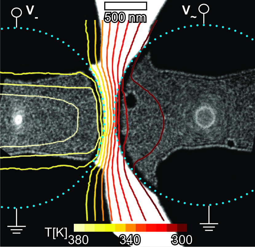
Figure 1: Lorentz Transmission electron microscopy images of the excited double disk structure. LTEM image of the pair of magnetic vortex oscillators with a radius of $r=\text{$0.9\text{\,}\mathrm{\SIUnitSymbolMicro m}$}$. The vortex gyration modes are driven by a cw excitation at $239\text{\,}\mathrm{MHz}$ applied to the right disk ($disk_{d}$). The trajectories of the vortex core motion recorded in the DC mode of the LTEM can be observed as bright ellipses at the centers of both disks. A DC voltage $U_{heat}$ can be applied to the left ”heated” disk ($disk_{h}$). $U_{heat}$ is varied between $0\text{\,}\mathrm{V}0.4\text{\,}\mathrm{V}$ to manipulate the phase. In addition, the contour lines of the temperature distribution at $U_{heat}=\text{$0.4\text{\,}\mathrm{V}$}$ are plotted as can be seen, the driven disk ($disk_{d}$) remains at ambient temperature.

The magnetic vortex structure Ivanov and Zaspel (2004); Guslienko et al. (2006) is characterized by an in-plane curling magnetization; its sense of rotation defines the chirality $c=\pm 1$. Additionally, the magnetization direction of the perpendicularly magnetized vortex core (up or down) defines the polarity $p=\pm 1$. For disk shaped soft magnetic elements this magnetization structure causes flux closure of the in-plane magnetization with only the out-of-plane core with a size of $10\text{\,}\mathrm{nm}30\text{\,}\mathrm{nm}$ generating a small stray field Sugimoto et al. (2011). However, in the low frequency excitation state - called the gyration mode Sugimoto et al. (2011); Ivanov and Zaspel (2004) - surface magnetic charges appear. In case of a pair of vortices in close vicinity, this leads to a mutual dynamic dipolar interaction Novosad et al. (2005); Choe (2004). Here, we investigate a system of two nominally identical Permalloy disks (radius $r=\text{$0.9\text{\,}\mathrm{\SIUnitSymbolMicro m}$}$, thickness $d=\text{$50\text{\,}\mathrm{n}\mathrm{m}$}$ ) placed next to each other on a thin $30\text{\,}\mathrm{nm}$ SiN-membrane required to perform LTEM and STXM measurements. The DC mode of LTEM is used to image the trajectories of the vortex cores Pollard et al. (2012) in order to determine their radius and eccentricity as a function of the frequency of the applied rf current. In addition, STXM is used to obtain time resolved images Bolte et al. (2008) of the vortex core motion in order to be able to determine the phase relation between the two coupled vortex core oscillators.

.1 Eigenmodes of the coupled oscillator system

The oscillators are excited by a cw excitation in the range of several hundred MHz applied to the right driven disk ($disk_{d}$) harnessing the Spin Transfer Torque effect (STT) Bretzner and Lindeberg (1998), see fig.1. To manipulate the phase a DC voltage $U_{heat}$ can be applied to the left ”heated” disk ($disk_{h}$) to change its temperature via Joule heating and thereby reducing its saturation magnetization $M_{S}$. The temperature of the heated disk can be estimated by $T_{h}=T_{0}+\frac{R_{thermal}}{R_{d}+R_{c}}U_{heat}^{2}$ with $T_{0}=\text{$293\text{\,}\mathrm{K}$}$ being ambient temperature, $R_{d}=\text{$90\text{\,}\Omega$}$ the electrical resistance of the disk, and $R_{c}$ the resistance of the electrical contacts. $R_{thermal}=63300\frac{K}{W}$ is the thermal resistance calculated using 3D finite elements methods (FEM). The right $disk_{d}$ stays close to ambient temperature as shown by the 3D FEM simulations (see fig. 1), which can be explained by the low thermal conductivity through the thin SiN membrane.
The dynamics of this system can be modeled using two coupled Thiele equations Thiele (1974); Lee et al. (2011a), which describe the dynamics of the vortex core positions for the driven (index $d$) and the heated (index $h$) disk. For $disk_{d}$ a spin polarized current density has been included Thiaville et al. (2005); Krueger et al. (2007):

$$\overrightarrow{G}_{d}\times(\overrightarrow{V}_{d}+b_{j}\overrightarrow{j})+\hat{D}_{d}(\alpha\overrightarrow{V}_{d}+\xi b_{j}\overrightarrow{j}) = \nabla_{\overrightarrow{R}_{d}}W(\overrightarrow{R}_{d},\overrightarrow{R}_{h})$$

$$\overrightarrow{G}_{h}\times\overrightarrow{V}_{h}+\hat{D}_{h}\alpha\overrightarrow{V}_{h} = \nabla_{\overrightarrow{R}_{h}}W(\overrightarrow{R}_{d},\overrightarrow{R}_{h}),$$

where $\overrightarrow{R}_{i}=(x_{i},y_{i}),i\in\{d,h\}$ is the vortex core displacement vector from the center of the disk $i$ and $\overrightarrow{V}_{i}=d\overrightarrow{R}_{i}/dt$ is the corresponding velocity vector. $b_{j}=P\mu_{B}/[eM_{S,d}(1+\xi^{2})]$ is the coupling constant between the applied current density $\overrightarrow{j}$ and the magnetization, where $P$ is the spin polarization of the conduction electrons, and $\xi$ the degree of nonadiabaticity Zhang and Li (2004). The corresponding gyro-vectors, $\overrightarrow{G}_{i}=-2\pi M_{S,i}\mu_{0}tp_{i}/\gamma\widehat{e}_{z}$, indicate the axes of precession perpendicular to the film plane. Here $M_{Si}$ is the saturation magnetization, $p_{i}$ the polarity of the corresponding vortex, $\mu_{0}$ the vacuum permeability, $t$ the sample thickness, and $\gamma$ the gyromagnetic ratio. The two diagonal dissipation tensors are indicated by $\hat{D}_{d}$ and $\hat{D}_{h}$. In the coupled system the total potential energy can be written as $W(\overrightarrow{R}_{d},\overrightarrow{R}_{h})=W_{0}+\kappa/2(\overrightarrow{R}_{d}^{2}+\overrightarrow{R}_{h}^{2})+c_{d}c_{h}(\eta_{x}x_{d}x_{h}-\eta_{y}y_{d}y_{h})$. The first constant term represents the potential energy for a central core position, i.e. $\overrightarrow{R}_{i}=(0,0)$. The second term represents the stray field energy and for small deflections can be modeled as a parabolic potential Guslienko et al. (2006) with stiffness coefficient $\kappa$. The third term reflects the magnetostatic energy between the side surfaces of the two disks Shibata et al. (2003), where $\eta_{x}$ and $\eta_{y}$ express the coupling strength along the $x$ and $y$ direction and $c_{i}$ being the chirality of the corresponding vortex.

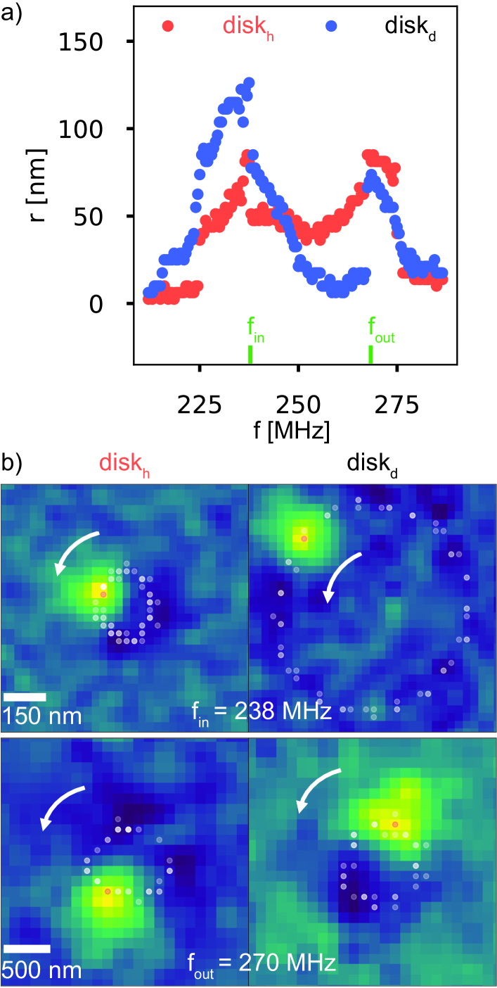
Figure 2: Resonance frequencies and time resolved imaging. a) Radius of both vortex core trajectories retrieved from LTEM measurement as a function of driving frequency. For each disk two resonances are observed corresponding to the in-phase and out-of-phase resonances of the coupled system. b) STXM measurements at $f_{in}$ (upper panels) and $f_{out}$ (lower panels) with respective phase shifts of $16.4\text{\,}\mathrm{MHz}$ and $176.3\text{\,}\mathrm{M}\mathrm{H}\mathrm{z}$ between the positions of the two vortex cores. The white circles represent the positions of the vortex cores as determined from the full image series. The red dots mark the positions of the vortex cores for the four images shown here.

To experimentally determine the two resonance frequencies of the coupled resonators and match the calculated data to the experiment, frequency swept LTEM measurements were performed. A cw excitation of $0.15\text{\,}\mathrm{V}$ was applied to $disk_{d}$ and the frequency was varied from $f=\text{$200\text{\,}\mathrm{MHz}300\text{\,}\mathrm{MHz}$}$ in steps of $0.5\text{\,}\mathrm{MHz}$. For each frequency an image similar to fig. 1 was taken and the radius of gyration of both vortex cores was determined. When plotted against the applied frequency two resonance frequencies can be resolved as expected for the system of two coupled oscillators, see fig. 2. For the subsequent experiments described below we use $f_{in}=\text{$238\text{\,}\mathrm{M}\mathrm{H}\mathrm{z}$}$ and $f_{out}=\text{$270\text{\,}\mathrm{M}\mathrm{H}\mathrm{z}$}$ as the in-phase and out-of-phase resonances, respectively. As shown in the supplementary information the method of phase manipulation presented here is robust against small deviations of the driving frequency from the resonant condition (see fig S1).

.2 Determination of the phase relation between the two coupled oscillators

To further investigate the phase relation between the two oscillators time-resolved STXM measurements at the MAXYMUS Beamline at Bessy II in Berlin were performed. First $disk_{d}$ was excited by a $0.15\text{\,}\mathrm{V}$ cw excitation at the two previously determined resonance frequencies ($f_{in}=\text{$238\text{\,}\mathrm{M}\mathrm{H}\mathrm{z}$}$ and $f_{out}=\text{$270\text{\,}\mathrm{M}\mathrm{H}\mathrm{z}$}$). The gyration was resolved with a time resolution of $66\text{\,}\mathrm{ps}$ leading to a series of 62 images. The bright spot on the dark background is a direct image of the $z$-component of the magnetization $M_{z}$ and allows to determine the polarities $p_{d}=p_{h}=1$. The sense of rotation for both disks is counter clockwise (ccw) and hence, the chirality can be determined to be $c_{d}=c_{h}=1$ Lee et al. (2011b), which serves as an input for the simulations. The positions of the vortex cores were tracked by the Laplacian of Gaussian method Bretzner and Lindeberg (1998) and are overlaid on the image as white spots for all 62 measurements, with the position of the shown image colored in red. This data can be plotted against time and fitted by a least squares sinusoidal fit with a fixed frequency equal to the excitation frequency. From the fit the phase between the two disks is retrieved together with the error from the covariance matrix. The error for the vortex core position is estimated by $\Delta_{x,y}=\pm\text{$50\text{\,}\mathrm{nm}$}$. Further the eccentricity $e=A_{x}/A_{y}$ of the elliptical trajectory is calculated.

	Phase [ ∘]		Eccentricity
$U_{heat}[V]$	f[MHz]	$\varphi_{exp}$	$\varphi_{th}$	$e_{h,exp}$	$e_{d,exp}$	$e_{h,th}$	$e_{d,th}$
0	238	$16.4\pm 7$	15	0.80	0.88	0.95	096
0	270	$176.3\pm 8$	176	1.12	1.02	1.05	1.04
0.43	238	$167.1\pm 12$	169.5	1.11	0.95	$>1$	$<1$

Table 1: Experimentally retrieved phase and eccentricity compared to calculated values determined by the extended Thiele equation model.

The measured phases (see table 1) are in excellent agreement with the results from the calculations. The change of the eccentricity from $e<1$ to $e>1$ from the in-phase resonance to the out-of-phase resonance is typical Lee et al. (2011b).

.3 Phase manipulation

Now, to manipulate the phase relation between the vortex core trajectories, a voltage $U_{heat}$ is applied to $disk_{h}$. The increase of temperature causes a decrease of the saturation magnetization $M_{S,h}$ of $disk_{h}$ while $M_{S,d}$ remains constant. $U_{heat}$ is increased stepwise from $0\text{\,}\mathrm{V}0.43\text{\,}\mathrm{V}$ while the frequency of the excitation is kept constant at $239\text{\,}\mathrm{M}\mathrm{H}\mathrm{z}$. For each heating voltage a series of images with the same time resolution is captured (see fig. 3 a)) and the phase is determined from the image series. The results are summarized in fig. 3 b) with $U_{heat}$ being the upper axis. The series starts again at a phase of $16.4^{\circ}$ for $U_{heat}=\text{$0\text{\,}\mathrm{V}$}$ and as can be seen the phase shifts up to a maximum of $167^{\circ}$ for $U_{heat}=\text{$0.4\text{\,}\mathrm{V}$}$ caused by a temperature increase of $disk_{d}$ of up to $85\text{\,}\mathrm{K}$. At the highest applied voltage the vortices are almost on the opposite side of the elliptical trajectory in contrast to the small phase shift observed for $U_{heat}=\text{$0\text{\,}\mathrm{V}$}$ (see fig. 3 a) and b)). In the simulation the largest observed phase shift corresponds to a ratio of $M_{S,h}/M_{S,d}=0.85$, see lower axis of fig. 3 b). To match the experimentally retrieved phase data for different temperatures to the analytically calculated phase values depending on the ratio $M_{S,h}/M_{S,d}$, the temperature dependence of $M_{S,h}(T)/M_{S,d}$ can be estimated via Bloch’s law Ashcroft and Mermin (1976): $M_{S,h}(T)=M_{0}(1-(\frac{T}{T_{c}})^{\frac{3}{2}})=M_{0}(1-(\frac{T0+\beta U_{heat}^{2}}{T_{c}})^{\frac{3}{2}})$. By doing so, the Curie temperature $T_{c}$ can be used as a parameter in a least square fit of the calculated phase to the experimentally retrieved values. Obviously, this is a very indirect method of determining $T_{c}$, however, the obtained value of $T_{c}=\text{$885\text{\,}\mathrm{K}$}\pm\text{$200\text{\,}\mathrm{K}$}$ is in good agreement with literature values Yu et al. (2008) and serves merely as a sanity check for the analytic modeling. The resulting dependence of the phase as a function of $M_{S,h}/M_{S,d}$ (fig. 3 b)) is in good agreement with theory. When going from the ”in-phase” to the ”out-of-phase” mode via manipulation of $M_{S,h}$ the eccentricity of $disk_{d}$ crosses from $e<1$ to $e>1$; the values change from $0.8$ to $1.11$. For $disk_{d}$ the eccentricity stays below 1 and changes from $0.88$ to $0.95$. Both observations are in good agreement with the simulations (see table 1). The complete transition is shown in fig. S2.

.4 Conclusions

In summary, we have successfully shown fine-grain phase manipulation of a pair of magnetic vortex oscillators in a controlled manner with high resolution (basically only limited by the measurement time) by a simple DC voltage input. The measurements were carried out at $239\text{\,}\mathrm{M}\mathrm{H}\mathrm{z}$ but vortex dynamics are easily scalable from the kHz to the GHz regime Noske et al. (2014). The power needed to control the phase is significant at $1.7\text{\,}\mathrm{m}\mathrm{W}$ but scales down orders of magnitudes when going to nano-oscillators. Moreover, we have developed a method of analog phase programming over a wide range from $16.4^{\circ}$ of up to $167^{\circ}$. The used method for phase programming relies solely on the oscillatory behavior of coupled oscillators, and the temperature dependence of the saturation magnetization. Hence, it allows for variable phase programming by a simple DC voltage input in a wide range of geometries and applications that can help advance the efforts of high frequency neuromorphic spintronics up to the GHz regime.

Acknowledgements: The authors gratefully acknowledge financial support by the DFG within the SpinCaT Priority Program (SPP 1538). Part of this work was supported by National Science Foundation Faculty Early Career Development Program (NSF-CAREER) Grant No. 1452670. We would like to thank M. Weigand for help with the STXM experiments. We would also like to acknowledge A. Hoffmann for fruitful discussions.

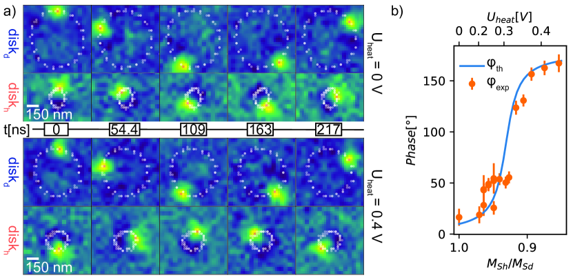
Figure 3: Phase control of the coupled oscillators. a) STXM image series for $f_{ex}=\text{$239\text{\,}\mathrm{MHz}$}$ and $U_{heat}=\text{$0\text{\,}\mathrm{V}$}$ (top) as well as $U_{heat}=\text{$0.43\text{\,}\mathrm{V}$}$ (bottom). For $U_{heat}=\text{$0\text{\,}\mathrm{V}$}$ the phase difference between both oscillators is $16.4^{\circ}\pm 7^{\circ}$ . For $U_{heat}=\text{$0.43\text{\,}\mathrm{V}$}$ the phase is increased to $167.1^{\circ}\pm 12^{\circ}$, and the cores are almost on the opposite side of the trajectory. Only 5 out of the 62 frames are plotted. All vortex core positions are overlaid in white. b) The phase $\varphi_{ex}$ retrieved from STXM data is plotted against $U_{heat}$ and the corresponding ratio of $\frac{M_{Sh}}{M_{Sd}}$. It agrees with the calculated phase change $\varphi_{th}$.

Supplemental Materials: Phase programming in coupled spintronic oscillators

I Phase programming in slight off resonant excitation

To study the influence of slight deviations $\Delta f$ of the driving frequency from the first resonant frequency $f_{in}$ to the first peak in the frequency spectra further analytically simulations using the coupled Thiele equation model have been carried out. Here $disk_{d}$ is driven by an AC current which has an amplitude of $5\times 10^{9}\textrm{ A}/\textrm{m}^{2}$ at a fixed frequency $f_{in}+\Delta f$. The heating of $disk_{h}$ is included by changing the saturation magnetization $M_{sh}$ of $disk_{h}$, while the saturation magnetization $M_{sd}$ of the driven disk is kept constant. As a result one can analyze the resulting phase shift between the gyrotropic motion of the coupled vortices as a function of the ratio of the saturation magnetizations $M_{sh}/M_{sd}$ in combination with different values for $\Delta f$ (see fig. S1). The overall behavior of the phase shift is independent on the size of $\Delta f$, as is the final phase shift at small ratios of $M_{sh}/M_{sd}$ (high heating powers). However, within the transition zone the phase shift dependends sensitively on the size of $\Delta f$.

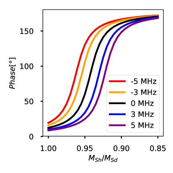
Figure S1: Phase manipulation for slightly off-resonant excitation. Calculated phase difference for the two vortex gyrations as a function of the saturation magnetization ratio $\frac{M_{sh}}{M_{sd}}$ of the heated disk and the driven disk for excitation frequencies shifted by $\Delta f$ from the first resonance of the coupled system shown for ($\Delta f=$-5\text{\,}\mathrm{M}\mathrm{H}\mathrm{z}$$, $-3\text{\,}\mathrm{M}\mathrm{H}\mathrm{z}$, $0\text{\,}\mathrm{M}\mathrm{H}\mathrm{z}$, $3\text{\,}\mathrm{M}\mathrm{H}\mathrm{z}$ and $5\text{\,}\mathrm{M}\mathrm{H}\mathrm{z}$). Data derived from a model of coupled Thiele equations.

II Dependence of the eccentricity on phase difference

As shown in table 1 in the main text the transition from the in-phase to the out of-phase-state by heating $disk_{h}$ is combined by a change of the eccentricity from $e_{h}<1$ to $e_{h}>1$ for $disk_{h}$ while the eccentricity of the excitation in $disk_{d}$ does not. The change of the eccentricity from $e>1$ to $e<1$ indicates a change in the overall elongation of the ellipse. If $e>1$ the ellipse is elongated along the $x$-axis, and if $e<1$ the ellipse is elongated along the $y$-axis. This behavior is also reproduced by the simulation derived from the coupled Thiele equation model (see solid lines in fig. S2). During the shift from the in-phase excitation to the out-of-phase sate the eccentricity of the driven disk only exhibits a value greater than $1$ over a limited phase range. For larger phase shifts the excitation again becomes elongated along the $y$-axis. The eccentricity of the vortex core gyration in the heated changes from values below 1 to values above 1. The change from values below 1 to values above 1 takes place around a phase difference of $90^{\circ}$. The eccentricity as well as the phase difference are two experimentally accessible values and can be directly compared with the experimental results (see crosses in fig. S2). The error for the phase is the same as in fig. 3 b). The error of the eccentricity follows from the error of the recorded values for the two axes $A_{x}$ and $A_{y}$ of the elliptical excitation by error-propagation. As can be seen $e_{d,exp}$ stays below a value of 1 (green line) for the described transition between the two states. The eccentricity $e_{h,exp}$ of the heated disk $disk_{h}$ on the other hand changes from $e_{h,exp}<1$ for phase shifts below $90^{\circ}$ to $e_{h,exp}>1$ for phase shifts above $90^{\circ}$. This agrees with the prediction from the simulations. Due to the nature of the sharp phase transition depending on the applied heating power (see fig. 3 b). The exact transition is experimentally hard to resolve.

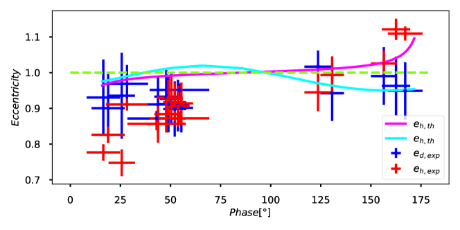
Figure S2: Eccentricity of the elliptical vortex gyration. Eccentricity $e$ for the elliptical trajectory of the two vortex gyrations as a function of phase difference. The solid lines are the results derived from the simulations (cyan for $disk_{d}$ and magenta for $disk_{h}$). The eccentricity for the experimentally resolved elliptical trajectory of the two vortex gyrations together with the derived errors is shown as crosses. The eccentricity $e_{d,exp}$ for the driven disk $disk_{d}$ is shown in blue. For the heated disk $disk_{h}$ the eccentricity $e_{h,exp}$ is shown in red. To exemplify the change of $e_{h,exp}<1$ to $e_{h,exp}>$ the green line at $e=1$ is shown.

References

- Mead (1990) C. Mead, Proceedings of the IEEE 78, 1629 (1990).
- Torrejon et al. (2017) J. Torrejon, M. Riou, F. A. Araujo, S. Tsunegi, G. Khalsa, D. Querlioz, P. Bortolotti, V. Cros, K. Yakushiji, A. Fukushima, H. Kubota, S. Yuasa, M. D. Stiles, and J. Grollier, Nature 547, 428 (2017).
- LeCun et al. (2015) Y. LeCun, Y. Bengio, and G. Hinton, Nature 521, 436 (2015).
- Schneider et al. (2018) M. L. Schneider, C. A. Donnelly, S. E. Russek, B. Baek, M. R. Pufall, P. F. Hopkins, P. D. Dresselhaus, S. P. Benz, and W. H. Rippard, Science Advances 4, e1701329 (2018).
- Jaeger and Haas (2004) H. Jaeger and H. Haas, Science 304, 78 (2004), arXiv:arXiv:1011.1669v3 .
- Hoppensteadt and Izhikevich (1999) F. C. Hoppensteadt and E. M. Izhikevich, Physical Review Letters 82, 2983 (1999).
- Buzsaki (2006) G. Buzsaki, Rhythms of the Brain (Oxford University Press, 2006).
- Nikonov et al. (2015) D. E. Nikonov, G. Csaba, W. Porod, T. Shibata, D. Voils, D. Hammerstrom, I. A. Young, and G. I. Bourianoff, IEEE Journal on Exploratory Solid-State Computational Devices and Circuits 1, 85 (2015).
- Shibata et al. (2012) T. Shibata, R. Zhang, S. P. Levitan, D. E. Nikonov, and G. I. Bourianoff, in 2012 13th International Workshop on Cellular Nanoscale Networks and their Applications (IEEE, 2012) pp. 1–5.
- Grollier et al. (2016) J. Grollier, D. Querlioz, and M. D. Stiles, Proceedings of the IEEE 104, 2024 (2016).
- Crespi et al. (2008) A. Crespi, D. Lachat, A. Pasquier, and A. J. Ijspeert, Autonomous Robots 25, 3 (2008).
- Ijspeert (2008) A. J. Ijspeert, Neural Networks 21, 642 (2008).
- Sharad et al. (2013) M. Sharad, D. Fan, K. Yogendra, and K. Roy, 2013 3rd Berkeley Symposium on Energy Efficient Electronic Systems, E3S 2013 - Proceedings (2013), 10.1109/E3S.2013.6705865, arXiv:1206.3227 .
- Sharma et al. (2013) A. A. Sharma, K. Neelathalli, D. Marculescu, and E. Nurvitadhi, in 2013 IEEE International Conference on Acoustics, Speech and Signal Processing (IEEE, 2013) pp. 2693–2696.
- Robert Kozma, Robinson E. Pino (2012) G. Robert Kozma, Robinson E. Pino, Advances in Neuromorphic Memristor Science and Applications vol. 4 (Springer-Verlag, New York, NY, USA, 2012).
- Buzsaki (2004) G. Buzsaki, Science 304, 1926 (2004).
- Marder and Bucher (2001) E. Marder and D. Bucher, Current Biology 11, R986 (2001).
- Kim et al. (2010) H.-T. Kim, B.-J. Kim, S. Choi, B.-G. Chae, Y. W. Lee, T. Driscoll, M. M. Qazilbash, and D. N. Basov, Journal of Applied Physics 107, 023702 (2010).
- Shukla et al. (2015) N. Shukla, A. Parihar, E. Freeman, H. Paik, G. Stone, V. Narayanan, H. Wen, Z. Cai, V. Gopalan, R. Engel-Herbert, D. G. Schlom, A. Raychowdhury, and S. Datta, Scientific Reports 4, 4964 (2015).
- Sharma et al. (2015) A. A. Sharma, J. A. Bain, and J. A. Weldon, IEEE Journal on Exploratory Solid-State Computational Devices and Circuits 1, 58 (2015).
- Sugimoto et al. (2011) S. Sugimoto, Y. Fukuma, S. Kasai, T. Kimura, A. Barman, and Y. Otani, Physical Review Letters 106, 197203 (2011).
- Bretzner and Lindeberg (1998) L. Bretzner and T. Lindeberg, Computer Vision and Image Understanding 71, 385 (1998).
- Thiele (1974) A. A. Thiele, Journal of Applied Physics 45, 377 (1974).
- Lee et al. (2011a) K.-S. Lee, H. Jung, D.-S. Han, and S.-K. Kim, Journal of Applied Physics 110, 113903 (2011a).
- Ivanov and Zaspel (2004) B. A. Ivanov and C. E. Zaspel, Journal of Applied Physics 95, 7444 (2004).
- Guslienko et al. (2006) K. Y. Guslienko, X. F. Han, D. J. Keavney, R. Divan, and S. D. Bader, Phys. Rev. Lett. 96, 67205 (2006).
- Novosad et al. (2005) V. Novosad, F. Y. Fradin, P. E. Roy, K. S. Buchanan, K. Y. Guslienko, and S. D. Bader, Physical Review B 72, 024455 (2005).
- Choe (2004) S.-B. Choe, Science 304, 420 (2004).
- Pollard et al. (2012) S. Pollard, L. Huang, K. Buchanan, D. Arena, and Y. Zhu, Nature Communications 3, 1028 (2012).
- Bolte et al. (2008) M. Bolte, G. Meier, B. Krüger, A. Drews, R. Eiselt, L. Bocklage, S. Bohlens, T. Tyliszczak, A. Vansteenkiste, B. Van Waeyenberge, K. W. Chou, A. Puzic, and H. Stoll, Physical Review Letters 100, 176601 (2008).
- Thiaville et al. (2005) A. Thiaville, Y. Nakatani, J. Miltat, and Y. Suzuki, EPL (Europhysics Letters) 69, 990 (2005).
- Krueger et al. (2007) B. Krueger, A. Drews, M. Bolte, U. Merkt, D. Pfannkuche, and G. Meier, Phys. Rev. B 76, 224426 (2007).
- Zhang and Li (2004) S. Zhang and Z. Li, Physical Review Letters 93 (2004), 10.1103/PhysRevLett.93.127204.
- Shibata et al. (2003) J. Shibata, K. Shigeto, and Y. Otani, Phys. Rev. B 67, 224404 (2003).
- Lee et al. (2011b) K.-S. Lee, H. Jung, D.-S. Han, and S.-K. Kim, Journal of Applied Physics 110, 113903 (2011b).
- Ashcroft and Mermin (1976) N. W. Ashcroft and N. D. Mermin, Solid state physics (Holt, Rinehart and Winston, 1976).
- Yu et al. (2008) P. Yu, X. F. Jin, J. Kudrnovský, D. S. Wang, and P. Bruno, Physical Review B 77, 054431 (2008).
- Noske et al. (2014) M. Noske, A. Gangwar, H. Stoll, M. Kammerer, M. Sproll, G. Dieterle, M. Weigand, M. Fähnle, G. Woltersdorf, C. H. Back, and G. Schütz, Physical Review B 90, 104415 (2014).