Solution Refinement at Regular Points
of Conic Problems

Abstract

Most numerical methods for conic problems use the homogenous primal-dual embedding, which yields a primal-dual solution or a certificate establishing primal or dual infeasibility. Following Patrinos [STP18], we express the embedding as the problem of finding a zero of a mapping containing a skew-symmetric linear function and projections onto cones and their duals. We focus on the special case when this mapping is regular, i.e., differentiable with nonsingular derivative matrix, at a solution point. While this is not always the case, it is a very common occurrence in practice. We propose a simple method that uses LSQR, a variant of conjugate gradients for least squares problems, and the derivative of the residual mapping to refine an approximate solution, i.e., to increase its accuracy. LSQR is a matrix-free method, i.e., requires only the evaluation of the derivative mapping and its adjoint, and so avoids forming or storing large matrices, which makes it efficient even for cone problems in which the data matrices are given and dense, and also allows the method to extend to cone programs in which the data are given as abstract linear operators. Numerical examples show that the method almost always improves an approximate solution of a conic program, and often dramatically, at a computational cost that is typically small compared to the cost of obtaining the original approximate solution. For completeness we describe methods for computing the derivative of the projection onto the cones commonly used in practice: nonnegative, second-order, semidefinite, and exponential cones. The paper is accompanied by an open source implementation.

1 Conic problem and homogeneous primal-dual embedding

We consider a conic optimization problem in its primal (P) and dual (D) forms (see, e.g., [BV04, §4.6.1] and [BTN01]):

$$\begin{array}[]{lll}\text{(P)}&\operatorname{minimize}&c^{T}x\\ &\text{subject to}&Ax+s=b\\ &&s\in\mathcal{K}\end{array}$$ (1)

$$\begin{array}[]{lll}\text{(D)}&\operatorname{minimize}&b^{T}y\\ &\text{subject to}&A^{T}y+c=0\\ &&y\in\mathcal{K}^{*}.\end{array}$$ (2)

Here $x\in{\mbox{\bf R}}^{n}$ is the primal variable, $y\in{\mbox{\bf R}}^{m}$ is the dual variable, and $s\in{\mbox{\bf R}}^{m}$ is the primal slack variable. The set $\mathcal{K}\subseteq{\mbox{\bf R}}^{m}$ is a nonempty closed convex cone and the set $\mathcal{K}^{*}\subseteq{\mbox{\bf R}}^{m}$ is its dual cone, $\mathcal{K}^{*}=\big{\{}{y\in{\mbox{\bf R}}^{m}}~{}\big{|}~{}{\inf_{k\in\mathcal{K}}y^{T}k\geq 0}\big{\}}$. The problem data are the matrix $A\in{\mbox{\bf R}}^{m\times n}$, the vectors $b\in{\mbox{\bf R}}^{m}$, $c\in{\mbox{\bf R}}^{n}$ and the cone $\mathcal{K}$.

Applications of conic problems.

Conic problems are widely used in practice. Any convex optimization problem can be formulated as a conic problem [BTN01]. Popular convex optimization solvers, such as ecos [DCB13], scs [OCPB16], mosek [MOS17], sedumi [Stu99], solve problems formulated as conic problems. Convex optimization frameworks, such as yalmip [L0̈4], cvx [GB14, GB08], cvxpy [DB16], Convex.jl [UMZ⁺14], and cvxr [FNB17], let the user formulate a convex optimization problem in high level mathematical language and then transform it to a conic problem. Classes of problems of practical importance, such as financial portfolio optimization [BBD⁺17, BRB16] and power grid management [Tay15], are increasingly specified, and solved, as conic problems.

Optimality conditions.

Let $(x,y,s)\in{\mbox{\bf R}}^{n}\times{\mbox{\bf R}}^{m}\times{\mbox{\bf R}}^{m}$. If $(x,y,s)$ satisfies the optimality or Karush–Kuhn–Tucker (KKT) conditions

$$Ax+s=b,\quad A^{T}y+c=0,\quad s\in\mathcal{K},\quad y\in\mathcal{K}^{*},\quad s^{T}y=0,$$ (3)

then $(x,s)$ is primal optimal, $y$ is dual optimal, and we say that $(x,y,s)$ is a solution of the primal-dual pair 2.

Primal and dual infeasibility.

If $y$ satisfies

$$A^{T}y=0,\quad y\in\mathcal{K}^{*},\quad b^{T}y=-1,$$ (4)

then $y$ serves as a proof or certificate that the primal problem is infeasible (equivalently, the dual problem is unbounded). If $(x,s)$ satisfies

$$Ax+s=0,\quad s\in\mathcal{K},\quad c^{T}x=-1,$$ (5)

then the pair $(x,s)$ serves as a proof or certificate that the primal problem is unbounded (equivalently, the dual problem is infeasible).

Solving a conic program.

It is easy to show that 3 and 4 are mutually exclusive, and that 3 and 5 are mutually exclusive. For non-degenerate conic programs, 4 and 5 are also mutually exclusive. (There exist degenerate conic programs for which both 4 and 5 are feasible, but such problems do not arise in applications.) By solving the conic program 2, we mean finding a solution of 3, 4, or 5.

Homogenous self-dual embedding.

The homogenous self-dual embedding of 2, introduced by Ye and others (see, e.g., [YTM94] and [OCPB16]), can be used to solve a conic problem. The embedding is as follows:

$$Qu=v,\quad u\in\mathbfcal{K},\quad v\in\mathbfcal{K}^{*},\quad u_{m+n+1}+v_{m+n+1}>0,$$ (6)

where

$$\mathbfcal{K}={\mbox{\bf R}}^{n}\times\mathcal{K}^{*}\times{\mbox{\bf R}}_{+},\quad\mathbfcal{K}^{*}=\{0\}^{n}\times\mathcal{K}\times{\mbox{\bf R}}_{+},$$

and $Q$ is the skew-symmetric matrix

$$Q=\begin{bmatrix}0&A{{}^{T}}&c\\ -A&0&b\\ -c{{}^{T}}&-b{{}^{T}}&0\end{bmatrix}.$$

The homogeneous self-dual embedding 6 is evidently positive homogeneous.

Constructing a solution of the conic problem 2, from a solution of the homogeneous embedding 6 proceeds as follows. We partition $u$ as $u=(u_{1},u_{2},\tau)$, and $v$ as $v=(v_{1},v_{2},\kappa)$, with

$$u_{1}\in{\mbox{\bf R}}^{n},\quad u_{2}\in\mathcal{K}^{*},\quad\tau\geq 0,\quad v_{1}=0\in{\mbox{\bf R}}^{n},\quad v_{2}\in\mathcal{K},\quad\kappa\geq 0.$$

If $(u,v)$ satisfies 6 then we have

$$u^{T}v=u_{1}^{T}v_{1}+u_{2}^{T}v_{2}+\tau\kappa=u_{2}^{T}v_{2}+\tau\kappa=0,$$

from which we conclude that $u_{2}^{T}v_{2}=0$ and $\tau\kappa=0$. Thus, one of $\tau$ and $\kappa$ is positive, and the other is zero. We distinguish three cases.

• $\tau>0$. Then $x=u_{1}/\tau$, $y=u_{2}/\tau$, $s=v_{2}/\tau$ is a primal-dual solution of the conic program, i.e., they satisfy 3.

• $\kappa>0$ and $b^{T}u_{2}<0$. Then $y=u_{2}/(b^{T}u_{2})$ is a certificate of primal infeasibility, i.e., satisfies 4.

• $\kappa>0$ and $c^{T}u_{1}<0$. Then $x=u_{1}/(c^{T}u_{1})$, $s=v_{2}/(c^{T}u_{1})$ is a certificate of dual infeasibility, i.e., satisfies 5.

Any solution of the homogenous self-dual embedding 6 must fall in one of the above three cases. To see this, suppose $\kappa>0$. Then $\tau=0$ and the last equation in $v=Qu$ becomes $-c^{T}u_{1}-b^{T}u_{2}=\kappa>0$, which implies that at least one of $b^{T}u_{2}$ and $c^{T}u_{1}$ is negative. These correspond to the second and third cases. (If both are negative, the conic program is degenerate.)

A converse also holds.

• If $(x,y,s)$ satisfies 3, then $u=(x,y,1)$ and $v=(0,s,0)$ satisfy 6.

• If $y$ satisfies 4, then $u=(0,y,0)$ and $v=(0,0,1)$ satisfy 6.

• If $x$, $s$ satisfy 5, then $u=(x,0,0)$, $v=(0,s,1)$ satisfy 6.

2 The residual map

The conic complementarity set.

We define the conic complementarity set as

$$\mathcal{C}=\big{\{}{(u,v)\in\mathbfcal{K}\times\mathbfcal{K}^{*}}~{}\big{|}~{}{u^{T}v=0}\big{\}}.$$ (7)

$\mathcal{C}$ is evidently a closed cone, but not necessarily convex. We let $\Pi$ denote Euclidean projection on $\mathbfcal{K}$, and $\Pi^{*}$ denote Euclidean projection on $-\mathbfcal{K}^{*}$. We observe that (see, e.g., [Mor65])

$$\Pi^{*}=I-\Pi,$$ (8)

where $I$ denotes the identity operator.

Minty’s parametrization of the complementarity set.

The mapping $M:{\mbox{\bf R}}^{m+n+1}\to\mathcal{C}$ given by

$$M(z)=(\Pi z,-\Pi^{*}z)$$ (9)

is called the Minty parametrization of $\mathcal{C}$. It is a bijection, with inverse $M^{-1}:\mathcal{C}\to{\mbox{\bf R}}^{m+n+1}$

$$M^{-1}(u,v)=u-v.$$ (10)

(See, e.g., [Roc70, Corollary 31.5.1] or [BC17, Remark 23.23(i)].) Since $\Pi$ is (firmly) nonexpansive, we conclude that $M$ is Lipschitz continuous with constant $1$.

Using this parametrization of $\mathcal{C}$, we can express the self-dual embedded conditions 6 in terms of $z$ as

$$-\Pi^{*}z=Q\Pi z,\quad z_{m+n+1}\neq 0.$$ (11)

We slightly stretch our notation and say that $z\in{\mbox{\bf R}}^{m+n+1}$ is a solution of the homogenous self-dual embedding 6 if $M(z)$ is a solution.

Residual map.

We define the residual map $\mathcal{R}:{\mbox{\bf R}}^{m+n+1}\to{\mbox{\bf R}}^{m+n+1}$ by

$$\mathcal{R}(z)=Q\Pi z+\Pi^{*}z=((Q-I)\Pi+I)z.$$ (12)

The map $\mathcal{R}$ is positively homogenous and differentiable almost everywhere (see Appendix A).

Normalized residual.

The normalized residual map $\mathcal{N}:\{z\in{\mbox{\bf R}}^{m+n+1}\mid z_{m+n+1}\neq 0\}\to{\mbox{\bf R}}^{m+n+1}$ is given by

$$\mathcal{N}(z)=\mathcal{R}(z/|w|)=\mathcal{R}(z)/|w|,$$ (13)

where we use $w$ to denote $z_{m+n+1}$ to lighten the notation. The second equality follows from positive homogeneity of $\mathcal{R}$. Note that by 11, if $z\in{\mbox{\bf R}}^{m+n+1}$ satisfies the self-dual embedding 6, then $\mathcal{N}(z)=0$. Conversely, if $\mathcal{N}(z)=0$, then $z$ satisfies the self-dual embedding 6. The idea of formulating the homogeneous self-dual embedding problem as finding a zero of mapping has been used in other work, e.g., [STP18].

For $z\in{\mbox{\bf R}}^{m+n+1}$, with $w=z_{m+n+1}\neq 0$, we use $\|\mathcal{N}(z)\|_{2}$ as a practical measure of the suboptimality of $z$, i.e., how far $z$ deviates from being a solution of 6. We refer to $\|\mathcal{N}(z)\|_{2}$ as the normalized residual norm of a candidate $z$.

Derivatives of residual and normalized residual maps.

Let $z\in{\mbox{\bf R}}^{m+n+1}$ be such that $\Pi$ is differentiable at $z$. Then $\mathcal{R}$ is differentiable at $z$, with derivative

$$\mathsf{D}\mathcal{R}(z)=(Q-I)\mathsf{D}\Pi(z)+I.$$ (14)

Now suppose $z\in{\mbox{\bf R}}^{m+n+1}$, with $w\neq 0$. In view of 13 and 14, $\mathcal{N}$ is differentiable at $z$, with derivative

$$\mathsf{D}\mathcal{N}(z)=\frac{\mathsf{D}\mathcal{R}(z)}{w}-\frac{\mathcal{R}(z)}{w^{2}}e^{T}=\frac{(Q-I)\mathsf{D}\Pi(z)+I}{w}-\frac{((Q-I)\Pi+I)z}{w^{2}}e^{T},$$ (15)

where $e=(0,\ldots,0,1)\in{\mbox{\bf R}}^{m+n+1}$, and we remind the reader that $w=z_{m+n+1}$.

3 Cone projections and matrix-free derivative evaluations

Here we consider some of the standard cones used in practice, and for each one, describe the projection, and also how to evaluate its derivative mapping and its adjoint efficiently. Many of these results have appeared in other works [KFF09, AWK18, MS06, PB14]. We give them here for completeness, to put them in a common notation, and to point out how the derivative mappings can be efficiently evaluated.

Cartesian product of cones.

In many cases of interest the cone $\mathcal{K}$ is a Cartesian product of simpler closed convex cones, i.e., $\mathcal{K}=\mathcal{K}_{1}\times\cdots\times\mathcal{K}_{p}$. The projection $\Pi$ onto $\mathcal{K}$ is evidently the Cartesian product of the projections, $\Pi=\Pi_{\mathcal{K}_{1}}\times\cdots\times\Pi_{\mathcal{K}_{p}}$. It is clear that $\Pi$ is differentiable at $x=(x_{1},\ldots,x_{p})$ if and only if each $\Pi_{\mathcal{K}_{i}}$ is differentiable at $x_{i}$, and its derivative is

$$\mathsf{D}\Pi=\mathsf{D}\Pi_{\mathcal{K}_{1}}\times\cdots\times\mathsf{D}\Pi_{\mathcal{K}_{p}}.$$ (16)

(When the derivative is represented as a matrix, the Cartesian product here is a block diagonal matrix.)

So it suffices to discuss the simpler cones, where for simplicity of notation, we drop the subscript and refer to the (smaller) cones as $\mathcal{K}$.

The computational cost of the projection, and evaluating its derivative, on a Cartesian product of cones is the sum of the costs of the operations carried out on each of the individual cones. Also, these operations can be easily parallelized.

Zero and free cones.

For $\mathcal{K}=\{0\}$, we have $\Pi x=0$; $\Pi$ is differentiable everywhere and, for every $x\in{\mbox{\bf R}}$, $\mathsf{D}\Pi(x)=0$. For $\mathcal{K}={\mbox{\bf R}}$, $\Pi x=x$; $\Pi$ is differentiable everywhere and, for every $x\in{\mbox{\bf R}}$, $\mathsf{D}\Pi(x)=1$.

Nonnegative cone.

For the nonnegative cone ${\mbox{\bf R}}_{+}$ the projection is given by $\Pi x=\max(x,0)$. It is differentiable for $x\neq 0$, with derivative $\mathsf{D}{\Pi}(x)=\tfrac{1}{2}(\mathbf{sign}(x)+1)$.

Second-order cone.

For the second-order cone (also known as the Lorentz cone)

$$\mathcal{K}=\{(t,x)\in{\mbox{\bf R}}_{+}\times{\mbox{\bf R}}^{n}\mid\|x\|_{2}\leq t\},$$ (17)

we have

$$\Pi(t,y)=\begin{cases}(t,y),&\text{~{}~{}if~{}~{}}\lVert y\rVert_{2}\leq t\\ (0,0),&\text{~{}~{}if~{}~{}}\lVert y\rVert_{2}\leq-t\\ \tfrac{t+\lVert y\rVert_{2}}{2}\big{(}1,{y}/{\lVert y\rVert_{2}}\big{)},&\text{~{}~{}otherwise}.\end{cases}$$ (18)

It follows from [KFF09, Lemma 2.5] that $\Pi$ is differentiable at $(t,x)$ whenever $\lVert x\rVert_{2}\neq|t|$, in which case we have

$$\mathsf{D}{\Pi}(t,x)=\begin{cases}I,&\text{~{}~{}if~{}~{}}\lVert x\rVert_{2}<t\\ 0,&\text{~{}~{}if~{}~{}}\lVert x\rVert_{2}<-t\\ \frac{1}{2\|x\|_{2}}\begin{bmatrix}\|x\|_{2}&x^{T}\\ x&({t}+\lVert x\rVert_{2})I-t\frac{x}{\|x\|_{2}}\frac{x^{T}}{\|x\|_{2}}\end{bmatrix},&\text{~{}~{}otherwise}.\end{cases}$$ (19)

(Note that $\mathsf{D}\Pi$ is symmetric, a consequence of $\mathcal{K}$ being self-dual.) Evaluating $\mathsf{D}\Pi(t,x)(\tilde{t},\tilde{x})$ efficiently is easy in the first two cases. In the third case one does not form the matrix, but rather evaluates it by computing $x^{T}\tilde{x}$, and then forming the result vector using vector operations. This requires a number of flops (floating point operations) that is linear in the dimension of the cone, as opposed to quadratic.

Semidefinite cone.

The semidefinite cone ${\mbox{\bf S}}^{n}_{+}$ is the cone of $n\times n$ positive semidefinite matrices. Let $X\in{\mbox{\bf S}}^{n}$ (the set of symmetric $n\times n$ matrices) and let

$$X=U\mathbf{diag}(\lambda)U^{T}$$ (20)

be its eigendecomposition, with $U^{T}U=I$ and $\lambda$ is the vector of eigenvalues of $X$. The projection of $X$ onto ${\mbox{\bf S}}^{n}_{+}$ is given by

$$\Pi X=U\mathbf{diag}(\lambda_{+})U^{T},$$ (21)

where $\lambda_{+}=\max(\lambda,0)$ (elementwise). It is known that (see, e.g., [MS06, Theorem 2.7]) $\Pi$ is differentiable at $X$ whenever $\det X\neq 0$. For $\det X\neq 0$, let $\mathsf{D}{\Pi}(X):{\mbox{\bf S}}^{n}\to{\mbox{\bf S}}^{n}$ be the derivative of $\Pi$ at $X$, and let $\widetilde{X}\in{\mbox{\bf S}}^{n}$. Then (see [MS06, Theorem 2.7] and also Appendix B below)

$$\mathsf{D}\Pi(X)(\widetilde{X})=U(B\circ(U^{T}\widetilde{X}U))U^{T},$$ (22)

where $\circ$ denotes the Hadamard (i.e., entrywise) product, and the symmetric matrix $B$ is given by

$$B_{ij}=\begin{cases}0,&\text{~{}~{}if~{}~{}}i\leq k,\,j\leq k;\\ \frac{(\lambda_{+})_{i}}{(\lambda_{-})_{j}+(\lambda_{+})_{i}},&\text{~{}~{}if~{}~{}}i>k,\,j\leq k;\\ \frac{(\lambda_{+})_{j}}{(\lambda_{-})_{i}+(\lambda_{+})_{j}},&\text{~{}~{}if~{}~{}}i\leq k,\,j>k;\\ 1,&\text{~{}~{}if~{}~{}}i>k,\,j>k.\end{cases}$$ (23)

(See 39.) This derivative is symmetric (self-adjoint) and is readily evaluated at $\tilde{X}$ using matrix-matrix products, which cost order $n^{3}$ flops. If we represent $X\in{\mbox{\bf S}}^{n}$ as a vector $x\in{\mbox{\bf R}}^{m}$, with $m={n(n+1)/2}$, the cost is order $m^{3/2}$.

The exponential cone.

The exponential cone is given by

$$\mathcal{K}=\{(x,y,z)\in{\mbox{\bf R}}^{3}~{}|~{}y\ e^{x/y}\leq z,~{}y>0\}\;\;\cup\;\;{\mbox{\bf R}}_{-}\times\{0\}\times{\mbox{\bf R}}_{+},$$ (24)

and its dual cone is given by

$$\mathcal{K}^{*}=\{(u,v,w)\in{\mbox{\bf R}}^{3}\mid u<0,~{}-ue^{v/u}\leq ew\}\;\;\cup\;\;\{0\}\times{\mbox{\bf R}}_{+}\times{\mbox{\bf R}}_{+}.$$ (25)

We have four cases (see [PB14, §6.3.4]):

• Case 1: $(x,y,z)\in\mathcal{K}$. Then $\Pi(x,y,z)=(x,y,z)$.

• Case 2: $(x,y,z)\in-\mathcal{K}^{*}\setminus\{(0,0,0)\}$. Then $\Pi(x,y,z)=(0,0,0)$.

• Case 3: $x<0$ and $y<0$. Then $\Pi(x,y,z)=(x,0,\max(z,0))$.

• Case 4: Otherwise, we have $\Pi(x,y,z)=(x^{*},y^{*},z^{*})$, where $(x^{*},y^{*},z^{*})$ is the unique solution of

  $$\begin{array}[]{ll}\text{minimize}&\|(x,y,z)-(\overline{x},\overline{y},\overline{z})\|_{2}^{2}\\ \text{subject to}&\overline{z}=\overline{y}e^{\overline{x}/\overline{y}},\ \overline{y}>0.\end{array}$$ (26)

The optimization problem 26 can be solved by a primal-dual Newton method (see [PB14, §6.3.4]). (The existence and uniqueness of $(x^{*},y^{*},z^{*})$ follow from the fact that $\mathcal{K}$ is closed and convex.) The derivative $\mathsf{D}\Pi$ is given in the following cases:

• Case 1: $(x,y,z)\in\mathbf{int}\ \mathcal{K}$. Then $\mathsf{D}\Pi(x,y,z)=(x,y,z)$.

• Case 2: $(x,y,z)\in-\mathbf{int}\ \mathcal{K}^{*}$. Then $\mathsf{D}\Pi(x,y,z)=(0,0,0)$.

• Case 3: $x<0$, $y<0$ and $z\neq 0$. Then $\mathsf{D}\Pi(x,y,z)=(1,0,\tfrac{1}{2}(1+\operatorname{sign}(z)))$.

• Case 4: $(x,y,z)\in\mathbf{int}\ ({\mbox{\bf R}}^{3}\setminus(\mathcal{K}\cup\mathcal{K^{*}}\cup{\mbox{\bf R}}_{-}\times{\mbox{\bf R}}_{-}\times{\mbox{\bf R}}))$. See the system of equations (47) below.

4 Refinement

Suppose that $\hat{z}\in{\mbox{\bf R}}^{m+n+1}$, $\hat{z}_{m+n+1}\neq 0$, is a given approximate solution of the self-dual embedding 6, by which we mean that it has a small positive normalized residual norm $\lVert\mathcal{N}(\hat{z})\rVert_{2}$. Our goal is to refine the approximate solution, i.e., to produce a vector $\delta$ for which

$$\lVert\mathcal{N}(\hat{z}+\delta)\rVert_{2}<\lVert\mathcal{N}(\hat{z})\rVert_{2}$$ (27)

(and, implicitly, $\hat{z}_{m+n+1}+\delta_{m+n+1}\neq 0$). We refer to $z=\hat{z}+\delta$ as the refined (approximate) solution.

Related work.

Refinement of an approximate solution of an optimization problem is a very old idea; in linear programming, for example, it relies on guessing the active set and then solving a set of linear equations, see, e.g., [NW06, §16.5]. In more general conic problems, it was introduced in, e.g., [EGL97]. Refinement is used in numerical solvers, such as the quadratic programming solver OSQP [SBG⁺17], where it is called polishing.

Refinement approach.

Our approach to refinement requires the assumptions that $\Pi$ is differentiable at $\hat{z}$, hence $\mathcal{N}$ is differentiable at $\hat{z}$, and that $\mathsf{D}\mathcal{N}(\hat{z})$ is invertible. In other words, the normalized residual mapping is regular at the point $\hat{z}$. While this condition need not hold, it does in many practical cases.

With our assumption, $\|\mathcal{N}(z)\|_{2}^{2}$ is differentiable at $\hat{z}$. The condition 27 holds for $\lVert\delta\rVert$ sufficiently small, whenever $\delta$ is a descent direction of $\|\mathcal{N}(z)\|_{2}^{2}$ at $\hat{z}$, i.e.,

$$\delta^{T}(\mathsf{D}\mathcal{N}(\hat{z}))^{T}\mathcal{N}(\hat{z})<0.$$ (28)

Such a descent direction always exists, by our assumption that $\hat{z}$ is not a solution (i.e., $\mathcal{N}(\hat{z})\neq 0$) and $\mathsf{D}\mathcal{N}(\hat{z})$ is invertible; for example, $\delta=-t(\mathsf{D}\mathcal{N}(\hat{z}))^{T}\mathcal{N}(\hat{z})$, with $t>0$ sufficiently small. (This is the negative gradient descent direction.) There are many other ways to choose $\delta$ for which the descent condition 28 holds. We now propose a specific method to find a descent direction $\delta$.

Levenberg–Marquardt refinement.

The Levenberg–Marquardt nonlinear least squares method uses the direction $\delta$ that minimizes

$$\|\mathcal{N}(\hat{z})+\mathsf{D}\mathcal{N}(\hat{z})\delta\|_{2}^{2}+\lambda\|\delta\|_{2}^{2},$$ (29)

where $\lambda>0$ is a regularization parameter (see, e.g., [WH85, Nas00, BV18]). Many other methods for constructing a descent method could be used, for example Newton-type methods; see, e.g., [NW06, QS93, QS99, Jia99] and the references therein.

Levenberg–Marquardt refinement with truncated LSQR.

Finding a $\delta$ that minimizes 29 is a least squares problem; we propose to use the iterative algorithm LSQR [PS82], a variant of the conjugate gradient method, to find an approximate minimizer. Specifically, we run the LSQR algorithm for some number of steps, and use the resulting $\delta$ as our descent direction. Because $(\mathsf{D}\mathcal{N}(\hat{z}))^{T}\mathcal{N}(\hat{z})\neq 0$, it can be shown that $\delta$ obtained using this truncated LSQR method is a descent direction, i.e., 28 holds; see [LMW67].

We have two motivations for using LSQR to compute $\delta$. First, LSQR does not require forming the matrix $\mathsf{D}\mathcal{N}(\hat{z})$; it simply requires us to multiply a vector by it, and its transpose. This gives us all the computational advantages described in the previous section. The second reason is that with relatively few iterations of LSQR, a quite good descent direction is typically found.

Line search.

We take as our refined approximate solution $\hat{z}+t\delta$, where the step-size $t>0$ is obtained via backtracking line search [BV04, §9.2]. Specifically, we choose $t=2^{-p}$ where $p$ is the smallest nonnegative integer, not exceeding a given maximum $K>0$, for which $\|\mathcal{N}(\hat{z}+t\delta)\|_{2}<\|\mathcal{N}(\hat{z})\|_{2}$ holds (and, implicitly, $\hat{z}_{m+n+1}+t\delta_{m+n+1}\neq 0$). When $\|\mathcal{N}(\hat{z}+t\delta)\|_{2}<\|\mathcal{N}(\hat{z})\|_{2}$ fails to hold for $t=2^{-K}$, we exit the refinement process, using $t=0$, i.e., $z=\hat{z}$. We refer to this as a case of failed refinement. We find that $K=10$ is a good choice in practice; in almost all cases, far fewer backtracking steps are needed to produce a refined point.

Iterated refinement.

The refinement method described above can be iterated, provided that at each of the points produced, $\mathcal{N}$ is regular. One might even imagine that iterated refinement could be used to solve a conic problem, by starting from some arbitrary point with large normalized residual, and iteratively refining it. But we note that the regularity condition on the iterates need not hold, and even when they do, the method can fail to converge to a solution, and even when they converge to a solution, the convergence can be very slow. For these reasons we cannot recommend iterated refinement as a general method for solving a conic problem. We propose refinement, and iterated refinement, as nothing more than a method that can, and often does, produce a more accurate approximate solution, given an approximate solution produced by another method.

Refinement algorithm parameters.

Our refinement method has only a few parameters: The number of LSQR iterations to carry out to determine the descent direction $\delta$, the maximum number of backtracking steps in the line search, the regularization parameter $\lambda$, and the number of steps of refinement. Default values such as $30$ LSQR iterations, $10$ backtracking steps, $\lambda=10^{-8}$, and $2$ steps of iterated refinement seem to provide very good results across a variety of problem instances.

Computational complexity.

Here we summarize the computational complexity of our refinement method. Each LSQR iteration requires one matrix vector multiplication by $Q$, one by its transpose, one by $\mathsf{D}\mathcal{N}$, one by its transpose, and a few vector operations. Each evaluation of the residual function requires a multiplication by $Q$, one evaluation of $\Pi_{\mathcal{K}}$, and a few vector operations. These operations have costs that depend on the format of $A$ (e.g., dense or sparse) and the size and types of the cones that form $\mathcal{K}$. Using the default parameter values of 30 LSQR iterations and 2 steps of iterated refinement, we have $60$ (or fewer) LSQR iterations and between $3$ and $20$ evaluations of the normalized residual function.

More specific estimates depend on the structure of $A$ and $\mathcal{K}$. If $A$ is sparse with ${\text{\bf nnz}}{(A)}$ nonzero entries, multiplications by $Q$ and $Q^{T}$ cost roughly $\approx{\text{\bf nnz}}{(A)}+n+m$ flops. Perhaps the most expensive evaluations of the normalized residual, and its derivative, occur with $\mathcal{K}$ a single semidefinite cone. In this case, the projection $\Pi_{\mathcal{K}}$ and multiplications by $\mathsf{D}\mathcal{N}$ and its transpose require a number of flops proportional to $m^{3/2}$.

Reference implementation.

This paper is accompanied by a reference implementation, written in Python and available at

https://github.com/cvxgrp/cone_prog_refine.

The code implements the refinement method described in this paper, using Numpy [Oli06], Scipy [JOPO01], and Numba [Tea15], a just-in-time compiler, to run faster. Refining an approximate solution requires a single function call, with the problem data expressed in the same way used by the open source solvers ECOS [DCB13] and SCS [OCPB16]: $A$ is a sparse compressed-column matrix, $b$ and $c$ are Numpy arrays. The cone $\mathcal{K}$ is the Cartesian product of a sequence of zero, nonnegative, second order, semi-definite, and primal or dual exponential cones. We represent it with a Python dictionary containing the dimensions of the component cones.

5 Numerical experiments

We test the refinement algorithm on a variety of randomly generated problems, including feasible, infeasible, and unbounded problems. We report results obtained on an (Apple) laptop with a $2.7~{}$GHz quad-core processor and $16~{}$Gb of RAM. The Python environment used is the Anaconda distribution (with Python 3.7, Numpy 1.15, Scipy 1.1, and Numba 0.36). All the experiments can be reproduced by running the experiments.ipynb notebook (in the examples folder of the software repository).

Problem generation.

The random problem instances are generated as follows.

• The cone $\mathcal{K}$ is the Cartesian product of a zero cone of size random uniform in $\{10,\ldots,50\}$, a nonnegative cone of size random uniform in $\{20,\ldots,100\}$, a number of Lorentz cones random uniform in $\{2,\ldots,100\}$ where each has size random uniform in $\{5,\ldots,20\}$, a number of semi-definite cones random uniform in $\{5,\ldots,20\}$ where each has size random uniform in $\{2,\ldots,10\}$, and a number of primal, and dual, exponential cones both random uniform in $\{2,\ldots,10\}$. This determines the value of $m$, and we choose $n$ random uniform in $\{1,\ldots,m\}$. The (empirical) $10$th and $90$th quantiles of the distribution of $n$ and $m$ are about $(100,1000)$ and $(500,1500)$, respectively.

• The matrix $A$ has a random sparsity pattern with density chosen random uniformly in $[0.1,0.3]$. Its entries, and the entries of the optimal $x$ and $r=(s-y)$, are chosen random uniformly in $[-1,1]$. $A$ is then divided by its Frobenius norm, so that $\|A\|_{F}=1$. We compute $s=\Pi(r)$, and $y=s-r$. Then, we choose randomly between a feasible, infeasible, or unbounded problem, with probabilities 0.8, 0.1, and 0.1, respectively, and proceed as follows:

  • For a feasible problem instance, we set $b=Ax+s$, and $c=-A^{T}y$.

  • For an infeasible problem instance, for each column $j$ of $A$ we pick the first nonzero element, if there are any, say $A_{ij}$. We check that $y_{i}\neq 0$, and if not choose the next nonzero $A_{ij}$, and substitute $A_{ij}$ with $A_{ij}-(A^{T}y)_{j}/y_{i}$, so now $A^{T}y=0$. We then set $b=-y/\|y\|^{2}_{2}$, and $c$ with random uniform entries in $[-1,1]$.

  • For an unbounded problem instance, for any element $x_{j}$ of the solution $x$ that is zero, i.e., $x_{j}=0$, we set $x_{j}=1$. Then, for each row $i$ of $A$, we pick the first nonzero element, say $A_{ij}$, or, if there are none, $A_{i1}$. We substitute $A_{ij}$ with $A_{ij}-(Ax+s)_{i}/x_{j}$, so now $Ax+s=0$. We then set $c=-x/\|x\|^{2}_{2}$, and $b$ with random uniform entries in $[-1,1]$.

Experiments.

We generate $1000$ such problems, and for each we obtain an approximate solution (or a certificate of infeasibility or unboundedness) with the numerical solver SCS (if the cone includes semi-definite or exponential cones), or ECOS (otherwise). We then pass the approximate solution returned by the solver to the refinement algorithm, and obtain a refined approximate solution. We use default parameters for both the solvers and the refinement algorithm.

Figure 1: Residual norm of unrefined and refined approximate solutions, for the experiments of §5.

Results.

Figure 1 shows the scatter plot, for each problem, of $\|\mathcal{N}(z_{\text{unref}})\|_{2}$ against $\|\mathcal{N}(z_{\text{ref}})\|_{2}$, where $z_{\text{unref}}$ is the approximate solution returned by the solver and $z_{\text{ref}}$ is the refined solution returned by the refinement algorithm. We see that the refined solutions always have smaller residual norm than the unrefined ones, and sometimes significantly so. (More details can be seen in the experiments.ipynb notebook in the software repository.) Figure 2 shows the distribution of the refinement factor $\|\mathcal{N}(z_{\text{unref}})\|_{2}/\|\mathcal{N}(z_{\text{ref}})\|_{2}$, i.e., the change in solution quality before and after refinement. We see that in most cases the refinement algorithm improves the solution quality by about an order of magnitude, and sometimes by a few orders of magnitude. The geometric mean of the refinement factor over our 1000 problems is around 30.

Timing.

Using the default parameters, the time required for refinement of the 1000 example problems is either insignificant compared to the original solver, or comparable in some cases. For very small problems, for which the base solvers ECOS and SCS are very fast (in the few millisecond range), our current Python implementation of the refinement method requires (relatively) more time, but a C implementation of refinement would rectify this.

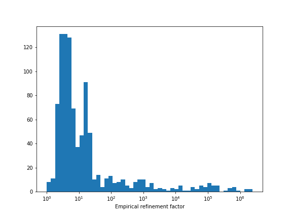
Figure 2: Distribution of refinement factor $\|\mathcal{N}(z_{\text{unref}})\|_{2}/\|\mathcal{N}(z_{\text{ref}})\|_{2}$ over the experiments of §5.

Appendix A

Differentiability properties of the residual map.

Let $C$ be a nonempty closed convex subset of ${\mbox{\bf R}}^{n}$. It is well known that the projection $\Pi_{C}$ onto $C$ is (firmly) nonexpansive (see, e.g., [Bro67, Proposition 2]), hence it is Lipschitz continuous with a Lipschitz constant at most $1$. Consequently, if $A:{\mbox{\bf R}}^{n}\to{\mbox{\bf R}}^{m}$ is linear then the composition $A\circ\Pi_{C}$ is also Lipschitz continuous. Therefore, by the Rademacher’s Theorem (see, e.g., [RW98, Theorem 9.60] or [EG92, Theorem 3.2]) both $\Pi_{C}$ and $A\circ\Pi_{C}$ are differentiable almost everywhere. This allows us to conclude that the residual map 12 is differentiable almost everywhere. Moreover, let $z\in{\mbox{\bf R}}^{m+n+1}$. Clearly $\mathcal{R}$ is differentiable at $z$ if $\Pi$ is differentiable at $z$.

Appendix B

Semi-definite cone projection derivative.

Let $X\in{\mbox{\bf S}}^{n}$, let $X=U\mathbf{diag}(\lambda)U^{T}$ be an eigendecomposition of $X$ and suppose that $\det(X)\neq 0$. Without loss of generality, we can and do assume that the entries of $\lambda$ are in an increasing order. That is, there exists $k\in\{1,\ldots,n\}$ such that

$$\lambda_{1}\leq\cdots\leq\lambda_{k}<0<\lambda_{k+1}\leq\cdots\leq\lambda_{n}.$$ (30)

We also note that

$$\Pi X-X=U\mathbf{diag}(\lambda_{-})U^{T},$$ (31)

where $\lambda_{-}=-\min(\lambda,0)$. It follows from 21, 31, and the orthogonality of $U$ that

$$U^{T}\Pi XU=\mathbf{diag}(\lambda_{+}),\quad U^{T}(\Pi X-X)U=\mathbf{diag}(\lambda_{-}).$$ (32)

Note that

$$\Pi X(\Pi X-X)=U\mathbf{diag}(\lambda_{+})\mathbf{diag}(\lambda_{-})U^{T}=0.$$ (33)

Let $\mathsf{D}{\Pi}(X):{\mbox{\bf S}}^{n}\to{\mbox{\bf S}}^{n}$ be the derivative of $\Pi$ at $X$, and let $\widetilde{X}\in{\mbox{\bf S}}^{n}$. We now show that 22 holds.

Indeed, using the first order Taylor approximation of $\Pi$ around $X$, for $\Delta X\in{\mbox{\bf S}}^{n}$ such that $\lVert\Delta X\rVert_{F}$ is sufficiently small (here $\lVert\cdot\rVert_{F}$ denotes the Frobenius norm) we have

$$\Pi(X+\Delta X)\approx\Pi X+\mathsf{D}\Pi(X)(\Delta X).$$ (34)

To simplify the notation, we set $\Delta Y=\mathsf{D}\Pi(X)(\Delta X)$. Now

$$0 =\Pi(X+\Delta X)(\Pi(X+\Delta X)-X-\Delta X)$$ (35a)

$$\approx(\Pi X+\Delta Y)(\Pi X+\Delta Y-X-\Delta X)$$ (35b)

$$=\Pi X(\Pi X-X)+\Delta Y(\Pi X-X)+\Pi X(\Delta Y-\Delta X)+\Delta Y(\Delta Y-\Delta X)$$ (35c)

$$=\Pi X(\Delta Y-\Delta X)+\Delta Y(\Pi X-X)$$ (35d)

$$=U^{T}\Pi X(\Delta Y-\Delta X)U+U^{T}\Delta Y(\Pi X-X)U$$ (35e)

$$=(U^{T}\Pi XU)U^{T}(\Delta Y-\Delta X)U+U^{T}\Delta YU(U^{T}(\Pi X-X)U)$$ (35f)

$$=\mathbf{diag}(\lambda_{+})U^{T}(\Delta Y-\Delta X)U+U^{T}\Delta YU(\mathbf{diag}(\lambda_{+})).$$ (35g)

Here, 35a follows from applying 33 with $X$ replaced by $X+\Delta X$, 35b follows from combining 35a and 34, 35d follows from 33 by neglecting second order terms, 35e follows from multiplying 35d from the left by $U^{T}$ and from the right by $U$, 35f follows from the fact that $UU^{T}=I$ and finally 35g follows from 32. We rewrite the Sylvester [Syl84, GLAM92] equation 35g as

$$\mathbf{diag}(\lambda_{+})U^{T}\Delta YU+U^{T}\Delta YU\mathbf{diag}(\lambda_{+})\approx\mathbf{diag}(\lambda_{+})U^{T}\Delta XU.$$ (36)

Using 36, we learn that for any $i\in\{1,\ldots,n\}$ and $j\in\{1,\ldots,n\}$, we have

$$((\lambda_{-})_{j}+(\lambda_{+})_{i})(U^{T}\Delta YU)_{ij}\approx(\lambda_{+})_{i}(U^{T}\Delta XU)_{ij}.$$ (37)

Recalling 30, if $i\leq k,\,j>k$ we have $(\lambda_{-})_{j}=(\lambda_{+})_{i}=0$. Otherwise, $(\lambda_{-})_{j}+(\lambda_{+})_{i}\neq 0$ and

$$(U^{T}\Delta YU)_{ij}\approx\underbrace{\frac{(\lambda_{+})_{i}}{(\lambda_{-})_{j}+(\lambda_{+})_{i}}}_{=B_{ij}}(U^{T}\Delta XU)_{ij}.$$ (38)

Proceeding by cases in view of 30, and using that $\Delta Y$ is symmetric (so is $U^{T}\Delta YU$), we conclude that

$$B_{ij}=\begin{cases}0,&\text{~{}~{}if~{}~{}}i\leq k,\,j\leq k;\\ \frac{(\lambda_{+})_{i}}{(\lambda_{-})_{j}+(\lambda_{+})_{i}},&\text{~{}~{}if~{}~{}}i>k,\,j\leq k;\\ \frac{(\lambda_{+})_{j}}{(\lambda_{-})_{i}+(\lambda_{+})_{j}},&\text{~{}~{}if~{}~{}}i\leq k,\,j>k;\\ 1,&\text{~{}~{}if~{}~{}}i>k,\,j>k.\\ \end{cases}$$ (39)

Therefore, combining with 38 we obtain

$$U^{T}\Delta YU\approx B\circ(U^{T}\Delta XU),$$ (40)

where “$\circ$” denotes the Hadamard (i.e., entrywise) product. Recalling the definition of $\Delta Y$ and using that $UU^{T}=I$ we conclude that

$$\mathsf{D}\Pi(X)(\Delta X)\approx U(B\circ(U^{T}\Delta XU))U^{T}.$$ (41)

Letting $\lVert\Delta X\rVert_{F}\to 0$ and applying the implicit function theorem, we conclude that 22 holds.

Appendix C

Exponential cone projection derivative.

The Lagrangian of the constrained optimization problem 26 is

$$\tfrac{1}{2}\lVert(x,y,z)-(\overline{x},\overline{y},\overline{z})\rVert^{2}+\mu(\overline{y}e^{\overline{x}/\overline{y}}-\overline{z}),$$ (42)

where $\mu\in{\mbox{\bf R}}$ is the dual variable. The KKT conditions at a solution $(x^{*},y^{*},z^{*},\mu^{*})$ are

$$x^{*}-x+\mu^{*}e^{x^{*}/y^{*}} =0$$ (43)

$$y^{*}-y+\mu^{*}e^{x^{*}/y^{*}}\big{(}1-\tfrac{x^{*}}{y^{*}}\big{)} =0$$ (44)

$$z^{*}-z-\mu^{*} =0$$ (45)

$$y^{*}e^{x^{*}/y^{*}}-z^{*} =0.$$ (46)

Considering the differentials $dx,dy,dz$ and $dx^{*},dy^{*},dz^{*},d\mu^{*}$ of the KKT conditions in 43, the authors of [AWK18, Lemma 3.6] obtain the system of equations

$$\underbrace{\begin{bmatrix}1+\tfrac{\mu^{*}e^{x^{*}/y^{*}}}{y^{*}}&-\tfrac{\mu^{*}x^{*}e^{x^{*}/y^{*}}}{{y^{*}}^{2}}&0&e^{x^{*}/y^{*}}\\ -\tfrac{\mu^{*}x^{*}e^{x^{*}/y^{*}}}{{y^{*}}^{2}}&1+\tfrac{\mu^{*}{x^{*}}^{2}e^{x^{*}/y^{*}}}{{y^{*}}^{3}}&0&(1-x^{*}/y^{*})e^{x^{*}/y^{*}}\\ 0&0&1&-1\\ e^{x^{*}/y^{*}}&(1-x^{*}/y^{*})e^{x^{*}/y^{*}}&-1&0\end{bmatrix}}_{D}\underbrace{\begin{bmatrix}dx^{*}\\ dy^{*}\\ dz^{*}\\ d\mu^{*}\end{bmatrix}}_{du^{*}}=\underbrace{\begin{bmatrix}dx\\ dy\\ dz\\ 0\end{bmatrix}}_{du}.$$ (47)

Note that, since 26 is feasible, $D$ is invertible. Therefore, $du^{*}=D^{-1}(du)$. Consequently, the upper left $3\times 3$ block matrix of $D^{-1}$ is the Jacobian of the projection at $(x,y,z)$ in Case 4.

References

- [AWK18] A. Ali, E. Wong, and J. Kolter. A semismooth Newton method for fast, generic convex programming. In Proceedings of the 34 International Conference on Machine Learning, pages 272–279, 2018.
- [BBD+17] S. Boyd, E. Busseti, S. Diamond, R. Kahn, K. Koh, P. Nystrup, and J. Speth. Multi-period trading via convex optimization. Foundations and Trends in Optimization, 3(1):1–76, 2017.
- [BC17] H. Bauschke and P. Combettes. Convex Analysis and Monotone Operator Theory in Hilbert Spaces. Springer, second edition, 2017.
- [BRB16] E. Busseti, E. Ryu, and S. Boyd. Risk-constrained Kelly gambling. Journal of Investing, 25(3):118–134, 2016.
- [Bro67] F. Browder. Convergence theorems for sequences of nonlinear operators in Banach spaces. Mathematische Zeitschrift, 100(3):201–225, 1967.
- [BTN01] A. Ben-Tal and A. Nemirovski. Lectures on Modern Convex Optimization. SIAM, 2001.
- [BV04] S. Boyd and L. Vandenberghe. Convex Optimization. Cambridge University Press, 2004.
- [BV18] S. Boyd and L. Vandenberghe. Introduction to Applied Linear Algebra – Vectors, Matrices, and Least Squares. Cambridge University Press, 2018.
- [DB16] S. Diamond and S. Boyd. CVXPY: A Python-embedded modeling language for convex optimization. Journal of Machine Learning Research, 16(83):1–5, 2016.
- [DCB13] A. Domahidi, E. Chu, and S. Boyd. ECOS: An SOCP solver for embedded systems. In Proceedings of the European Control Conference, pages 3071–3076, 2013.
- [EG92] L. Evans and R. Gariepy. Measure Theory and Fine Properties of Functions. CRC Press, 1992.
- [EGL97] L. El Ghaoui and H. Lebret. Robust solutions to least-squares problems with uncertain data. SIAM Journal on Matrix Analysis and Applications, 18(4):1035–1064, 1997.
- [FNB17] A. Fu, B. Narasimhan, and S. Boyd. CVXR: An R package for disciplined convex optimization. ArXiv e-prints: 1711.07582, 2017.
- [GB08] M. Grant and S. Boyd. Graph implementations for nonsmooth convex programs. In Recent Advances in Learning and Control, Lecture Notes in Control and Information Sciences, pages 95–110. Springer, 2008.
- [GB14] M. Grant and S. Boyd. CVX: Matlab software for disciplined convex programming, version 2.1. http://cvxr.com/cvx, March 2014.
- [GLAM92] J. Gardiner, A. Laub, J. Amato, and C. Moler. Solution of the Sylvester matrix equation . Association for Computing Machinery. Transactions on Mathematical Software, 18(2):223–231, 1992.
- [Jia99] H. Jiang. Global convergence analysis of the generalized Newton and Gauss-Newton methods of the Fischer-Burmeister equation for the complementarity problem. Mathematics of Operations Research, 24(3):529–543, 1999.
- [JOPO01] E. Jones, T. Oliphant, P. Peterson, and Others. SciPy: Open source scientific tools for Python. http://www.scipy.org/, 2001.
- [KFF09] C. Kanzow, I. Ferenczi, and M. Fukushima. On the local convergence of semismooth Newton methods for linear and nonlinear second-order cone programs without strict complementarity. SIAM Journal on Optimization, 20(1):297–320, 2009.
- [L0̈4] J. Löfberg. YALMIP: A toolbox for modeling and optimization in MATLAB. In Proceedings of the IEEE International Symposium on Computer Aided Control Systems Design, pages 284–289, 2004.
- [LMW67] L. Lasdon, S. Mitter, and A. Waren. The conjugate gradient method for optimal control problems. IEEE Transactions on Automatic Control, 12(2):132–138, 1967.
- [Mor65] J.-J. Moreau. Décomposition orthogonale d’un espace hilbertien selon deux cônes mutuellement polaires. Bulletin de la Société Mathématique de France, 93:273–299, 1965.
- [MOS17] MOSEK ApS. The MOSEK optimization toolbox for matlab manual, version 8.0 (revision 57), 2017.
- [MS06] J. Malick and H. Sendov. Clarke generalized Jacobian of the projection onto the cone of positive semidefinite matrices. Set-Valued Analysis, 14(3):273–293, 2006.
- [Nas00] S. Nash. A survey of truncated-Newton methods. Journal of Computational and Applied Mathematics, 124(1-2):45–59, 2000.
- [NW06] J. Nocedal and S. Wright. Numerical Optimization. Springer, second edition, 2006.
- [OCPB16] B. O’Donoghue, E. Chu, N. Parikh, and S. Boyd. Conic optimization via operator splitting and homogeneous self-dual embedding. Journal of Optimization Theory and Applications, 169(3):1042–1068, 2016.
- [Oli06] T. Oliphant. A guide to NumPy, volume 1. Trelgol Publishing USA, 2006.
- [PB14] N. Parikh and S. Boyd. Proximal algorithms. Foundations and Trends in Optimization, 1(3):123–231, 2014.
- [PS82] C. Paige and M. Saunders. LSQR: An algorithm for sparse linear equations and sparse least squares. ACM Transactions on Mathematical Software, 8(1):43–71, 1982.
- [QS93] L. Qi and J. Sun. A nonsmooth version of Newton’s method. Mathematical Programming, 58(3, Ser. A):353–367, 1993.
- [QS99] L. Qi and D. Sun. A survey of some nonsmooth equations and smoothing Newton methods. In Progress in Optimization, Applied Optimization, pages 121–146. 1999.
- [Roc70] R. Rockafellar. Convex Analysis. Princeton University Press, 1970.
- [RW98] R. Rockafellar and R. Wets. Variational Analysis. Springer, 1998.
- [SBG+17] B. Stellato, G. Banjac, P. Goulart, A. Bemporad, and S. Boyd. OSQP: An operator splitting solver for quadratic programs. ArXiv e-prints: 1711.08013, 2017.
- [STP18] L. Stella, A. Themelis, and P. Patrinos. Newton-type alternating minimization algorithm for convex optimization. IEEE Transactions on Automatic Control (to appear), 2018.
- [Stu99] J. Sturm. Using SeDuMi 1.02, a MATLAB toolbox for optimization over symmetric cones. Optimization Methods and Software, 11(1-4):625–653, 1999.
- [Syl84] J. Sylvester. Sur l’équation linéaire trinôme en matrices d’un ordre quelconque. Comptes Rendus de l’Académie des Sciences, 99:527–529, 1884.
- [Tay15] J. Taylor. Convex Optimization of Power Systems. Cambridge University Press, 2015.
- [Tea15] Numba Development Team. Numba. http://numba.pydata.org, 2015.
- [UMZ+14] M. Udell, K. Mohan, D. Zeng, J. Hong, S. Diamond, and S. Boyd. Convex optimization in Julia. SC14 Workshop on High Performance Technical Computing in Dynamic Languages, 2014.
- [WH85] S. Wright and J. Holt. An inexact Levenberg–Marquardt method for large sparse nonlinear least squares. The ANZIAM Journal, 26(4):387–403, 1985.
- [YTM94] Y. Ye, M. Todd, and S. Mizuno. An -iteration homogeneous and self-dual linear programming algorithm. Mathematics of Operations Research, 19(1):53–67, 1994.