How Many Pairwise Preferences Do We Need to Rank a Graph Consistently?

Abstract

We consider the problem of optimal recovery of true ranking of $n$ items from a randomly chosen subset of their pairwise preferences. It is well known that without any further assumption, one requires a sample size of $\Omega(n^{2})$ for the purpose. We analyze the problem with an additional structure of relational graph $G([n],E)$ over the $n$ items added with an assumption of locality: Neighboring items are similar in their rankings. Noting the preferential nature of the data, we choose to embed not the graph, but, its strong product to capture the pairwise node relationships. Furthermore, unlike existing literature that uses Laplacian embedding for graph based learning problems, we use a richer class of graph embeddings—orthonormal representations—that includes (normalized) Laplacian as its special case. Our proposed algorithm, Pref-Rank, predicts the underlying ranking using an SVM based approach over the chosen embedding of the product graph, and is the first to provide statistical consistency on two ranking losses: Kendall’s tau and Spearman’s footrule, with a required sample complexity of $O(n^{2}\chi(\bar{G}))^{\frac{2}{3}}$ pairs, $\chi(\bar{G})$ being the chromatic number of the complement graph $\bar{G}$. Clearly, our sample complexity is smaller for dense graphs, with $\chi(\bar{G})$ characterizing the degree of node connectivity, which is also intuitive due to the locality assumption e.g. $O(n^{\frac{4}{3}})$ for union of $k$-cliques, or $O(n^{\frac{5}{3}})$ for random and power law graphs etc.—a quantity much smaller than the fundamental limit of $\Omega(n^{2})$ for large $n$. This, for the first time, relates ranking complexity to structural properties of the graph. We also report experimental evaluations on different synthetic and real datasets, where our algorithm is shown to outperform the state-of-the-art methods.

1 Introduction

Table 1: Summary of sample complexities for ranking from pairwise preferences.

Reference	Assumption on the Ranking Model	Sampling Technique	Sample Complexity
Braverman and Mossel (2008)	Noisy permutation	Active	$O(n\log n)$
Jamieson and Nowak (2011)	Low $d$-dimensional embedding	Active	$O(d\log^{2}n)$
Ailon (2012)	Deterministic tournament	Active	$O(n\text{poly}(\log n))$
Gleich and Lim (2011)	Rank-$r$ pairwise preference with $\nu$ incoherence	Random	$O(n\nu r(\log n)^{2})$
Negahban et al. (2012)	Bradley Terry Luce (BTL)	Random	$O(n\log n)$
Wauthier et al. (2013)	Noisy permutation	Random	$O(n\log n)$
Rajkumar and Agarwal (2016)	Low $r$-rank pairwise preference	Random	$O(nr\log n)$
Niranjan and Rajkumar (2017)	Low $d$-rank feature with BTL	Random	$O(d^{2}\log n)$
Agarwal (2010)	Graph + Laplacian based ranking	Random	✗
Pref-Rank  (This paper)	Graph + Edge similarity based ranking	Random	$O(n^{2}\chi(\bar{G}))^{\frac{2}{3}}$

The problem of ranking from pairwise preferences has widespread applications in various real world scenarios e.g. web search Page et al. (1998); Kleinberg (1999), gene classification, recommender systems Theodoridis et al. (2013), image search Geng et al. (2009) and more. Its of no surprise why the problem is so well studied in various disciplines of research, be that computer science, statistics, operational research or computational biology. In particular, we study the problem of ranking (or ordering) of set of $n$ items, given some partial information of the relative ordering of the item pairs.

It is well known from the standard results of classical sorting algorithms, for any set of $n$ items associated to an unknown deterministic ordering, say ${\boldsymbol{\sigma}}_{n}^{*}$, and given the learner has access to only preferences of the item pairs, in general one requires to observe $\Omega(n\log n)$ actively selected pairs (where the learner can choose which pair to observe next) to obtain the true underlying ranking ${\boldsymbol{\sigma}}_{n}^{*}$; whereas, with random selection of pairs, it could be as bad as $\Omega(n^{2})$.

Related Work. Over the years, numerous attempts have been made to improve the above sample complexities by imposing different structural assumptions on the set of items or the underlying ranking model. In active ranking setting, Jamieson and Nowak (2011) gives a sample complexity of $O(d\log^{2}n)$, provided the true ranking is realizable in a $d$-dimensional embedding; Braverman and Mossel (2008) and Ailon (2012) proposed a near optimal recovery with sample complexity of $O(n\log n)$ and $O(n\text{poly}(\log n))$ respectively, under noisy permutation and tournament ranking model. For the non-active (random) setting, Wauthier et al. (2013) and Negahban et al. (2012) gave a sample complexity bound of $O(n\log n)$ under noisy permutation (with $O(\log n)$ repeated sampling) and BTL ranking model. Recently, Rajkumar and Agarwal (2016) showed a recovery guarantee of $O(nr\log n)$, given the preference matrix is rank $r$ under suitable transformation.

However, existing literature on sample complexity for graph based ranking problems is sparse, where it goes without saying that the underlying structural representation of the data is extremely relevant in various real world applications where the edge connections model item similarities e.g. In social network, connection among friends can be modelled as a graph, or in recommender systems, movies under same the genre should lie in close neighbourhood. It is important to note that a relational graph is different from imposing item dependencies through feature representations and much more practical, since side information of exact features may not even be available to the learner as required in the later case.

Furthermore, the only few algorithmic contributions made on the problem of ranking on graphs –  Page et al. (1998); He et al. (2017); Del Corso and Romani (2016); Hsu et al. (2017) have not explored their theoretical performance. Agarwal (2010, 2008) proposed an SVM-rank based algorithm, with generalization error bounds for the inductive and transductive graph ranking problems. Agarwal and Chakrabarti (2007) derived generalization guarantees for PageRank algorithm. To the best of our knowledge, we are not aware of any literature which provide statistical consistency guarantees to recover the true ranking and analyze the required sample complexity, which remains the primary focus of this work.

Problem Setting We precisely address the question: Given the additional knowledge of a relational graph on the set of $n$ items, say $G([n],E)$, can we find the underlying ranking ${\boldsymbol{\sigma}}_{n}^{*}$ faster (i.e. with a sample complexity lesser than $\Omega(n^{2})$)? Of course, in order to hope for achieving a better sample complexity, there must be a connection between the graph and the underlying ranking – question is how to model this?

A natural modelling could be to assume that similar items connected by an edge are close in terms of their rankings or similar node pairs have similar pairwise preferences. E.g. In movie recommendations, if two movies $A$ and $B$ belongs to thriller genre and $C$ belongs to comedy, and it is known that $A$ is preferred over $C$ (i.e. the true ranking over latent topics prefers thriller over comedy), then it is likely that $B$ would be preferred over $C$; and the learner might not require an explicit $(B,C)$ labelled pair – thus one can hope to reduce the sample complexity by inferring preference information of the neighbouring similar nodes. However, how to impose such a smoothness constraint remains an open problem.

One way out could be to assume the true ranking to be a smooth function over the graph Laplacian as also assumed in Agarwal (2010). However, why should we confine ourself to the notion of Laplacian embedding based similarity when several other graph embeddings could be explored for the purpose? In particular, we use a broader class of orthonormal representation of graphs for the purpose, which subsumes (normalized) Laplacian embedding as a special case, and assume the ranking to be a smooth function with respect to the underlying embedding (see Sec. 2.1 for details).

Our Contributions. Under the smoothness assumptions, we show a sample complexity guarantee of $O(n^{2}\chi(\bar{G}))^{\frac{2}{3}}$ to achieve ranking consistency – the result is intuitive as it indicates smaller sample complexity for densely connected graph, as one can expect to gather more information about the neighboring nodes compared to a sparse graph. Our proposed Pref-Rank algorithm, to the best of our knowledge, is the first attempt in proving consistency on large class of graph families with $\vartheta(G)=o(n)$, in terms of Kendall’s tau and Spearman’s footrule losses – It is developed on the novel idea of embedding nodes of the strong product graph $G\boxtimes G$, drawing inference from the preferential nature of the data and finally uses a kernelized-SVM approach to learn the underlying ranking. We summarize our contributions:

• The choice of graph embedding: Unlike the existing literature, which is restricted to Laplacian graph embedding Ando and Zhang (2007), we choose to embed the strong product $G\boxtimes G$ instead of $G$, as our ranking performance measures penalizes every pairwise misprediction; and use a general class of orthonormal representations, which subsumes (normalized) Laplacian as a special case.

• Our proposed preference based ranking algorithm: Pref-Rank is a kernelized-SVM based method that inputs an embedding of pairwise graph $G\boxtimes G$. The generalization error of Pref-Rank involves computing the transductive rademacher complexity of the function class associated with the underlying embedding used (see Thm. 3, Sec. 3).

• For the above, we propose to embed the nodes of $G\boxtimes G$ with $3$ different orthonormal representations: $(a)$ Kron-Lab($G\boxtimes G$)  $(b)$ PD-Lab($G$) and $(c)$ LS-labelling; and derive generalization error bounds for the same (Sec. 4).

• Consistency: We prove the existence of an optimal embedding in Kron-Lab($G\boxtimes G$) for which Pref-Rank is statistically consistent (Thm. 10, Sec. 5) over a large class of graphs, including power law and random graphs. To the best of our knowledge, this is the first attempt at establishing algorithmic consistency for graph ranking problems.

• Graph Ranking Sample Complexity: Furthermore, we show that observing $O(n^{2}\chi(\bar{G}))^{\frac{2}{3}}$ pairwise preferences a sufficient for Pref-Rank to be consistent (Thm. 12, Sec. 5.1), which implies that a densely connected graph requires much smaller training data compared to a sparse graph for learning the optimal ranking – as also intuitive. Our result is the first to connect the complexity of graph ranking problem to its structural properties. Our proposed bound is a significant improvement in sample complexity (for random selection of pairs) for dense graphs e.g. $O(n^{\frac{4}{3}})$ for union of $k$-cliques; and $O(n^{\frac{5}{3}})$ for random and power law graphs – a quantity much smaller than $\Omega(n^{2})$.

Our experimental results demonstrate the superiority of Pref-Rank algorithm compared to Graph Rank Agarwal (2010), Rank Centrality Negahban et al. (2012) and Inductive Pairwise Ranking Niranjan and Rajkumar (2017) on various synthetic and real-world datasets; validating our theoretical claims. Table 1 summarizes our contributions.

2 Preliminaries and Problem Statement

Notations. Let $[n]:=\{1,2,\ldots n\}$, for $n\in{\mathbb{Z}}_{+}$. Let $x_{i}$ denote the $i^{\text{th}}$ component of a vector ${\mathbf{x}}\in{\mathbb{R}}^{n}$. Let ${\mathbf{1}}\{\varphi\}$ denote an indicator function that takes the value $1$ if the predicate $\varphi$ is true and $0$ otherwise. Let ${\mathbf{1}}_{n}$ denote an $n$-dimensional vector of all $1$’s. Let $S^{n-1}=\big{\{}{\mathbf{u}}\in\mathbb{R}^{n}\big{|}\|{\mathbf{u}}\|_{2}=1\big{\}}$ denote a $(n-1)$ dimensional sphere. For any given matrix ${\mathbf{M}}\in{\mathbb{R}}^{m\times n}$, we denote the $i^{th}$ column by ${\mathbf{M}}_{i},\,\forall i\in[n]$ and $\lambda_{1}({\mathbf{M}})\geq\ldots\geq\lambda_{n}({\mathbf{M}})$ to denote its sorted eigenvalues, $tr({\mathbf{M}})$ to be its trace. Let ${\mathbf{S}}_{n}^{+}\in{\mathbb{R}}^{n\times n}$ denote $n\times n$ square symmetric positive semi-definite matrices. $G(V,E)$ denotes a simple undirected graph, with vertex set $V=[n]$ and edge set $E\subseteq V\times V$. We denote its adjacency matrix by $A_{G}$.

Orthonormal Representation of Graphs. Lovász (1979) An orthonormal representation of $G(V,E),~{}V=[n]$ is ${\mathbf{U}}=[{\mathbf{u}}_{1},\ldots,{\mathbf{u}}_{n}]\in\mathbb{R}^{d\times n}$ such that ${\mathbf{u}}_{i}^{\top}{\mathbf{u}}_{j}=0$ whenever $(i,j)\notin E$ and ${\mathbf{u}}_{i}\in{\mathbf{S}}^{d-1}~{}\forall i\in[n]$. Let $Lab(G)$ denote the set of all possible orthonormal representations of $G$ given by $Lab(G):=\{{\mathbf{U}}~{}|~{}{\mathbf{U}}\;\mbox{is an Orthonormal Representation}\}$. Consider the set of graph kernels $\mathcal{K}(G):=\{{\mathbf{K}}\in S^{+}_{n}~{}|~{}K_{ii}=1,\forall i\in[n];~{}K_{ij}=0,\forall(i,j)\notin E\}$. Jethava et al. (2013) showed the two sets to be equivalent i.e. for every ${\mathbf{U}}\in Lab(G)$, one can construct ${\mathbf{K}}\in{\mathcal{K}}(G)$ and vice-versa.

Definition 1.

Lovász Number. Lovász (1979) Orthonormal representations $Lab(G)$ of a graph $G$ is associated with an interesting quantity – Lovász number of $G$, defined as

$$\vartheta(G):=\min_{{\mathbf{U}}\in Lab(G)}\min_{{\mathbf{c}}\in S^{d-1}}\max_{i\in V}\frac{1}{({\mathbf{c}}^{\top}{\mathbf{u}}_{i})^{2}}$$

Lovász Sandwich Theorem: If $I(G)$ and $\chi(G)$ denote the independence number and chromatic number of the graph $G$, then $I(G)\leq\vartheta\left(G\right)\leq\chi(\bar{G})$ Lovász (1979).

Strong Product of Graphs. Given a graph $G=(V,E)$, strong product of $G$ with itself, denoted by $G\boxtimes G$, is defined over the vertex set $V(G\boxtimes G)=V\times V$, such that two nodes $(i,j),(i^{\prime},j^{\prime})\in V(G\boxtimes G)$ is adjacent in $G\boxtimes G$ if and only if $i=i^{\prime}$ and $(j,j^{\prime})\in E$, or $(i,i^{\prime})\in E$ and $j=j^{\prime}$, or $(i,i^{\prime})\in E$ and $(j,j^{\prime})\in E$. Also it is known from the classical work of Lovász (1979) that $\vartheta(G\boxtimes G)=\vartheta^{2}(G)$ (see Def. 15, Appendix for details).

2.1 Problem Statement

We study the problem of graph ranking on a simple, undirected graph $G=(V,E),~{}V=[n]$. Suppose there exists a true underlying ranking ${\boldsymbol{\sigma}}^{*}_{n}\in\Sigma_{n}$ of the nodes $V$, where $\Sigma_{n}$ is the set of all permutations of $[n]$, such that for any two distinct nodes $i,j\in V$, $i$ is said to be preferred over $j$ iff $\sigma_{n}^{*}(i)<\sigma_{n}^{*}(j)$. Clearly, without any structural assumption on how ${\boldsymbol{\sigma}}_{n}^{*}$ relates to the underlying graph $G(V,E)$, the knowledge of $G(V,E)$ is not very helpful in predicting ${\boldsymbol{\sigma}}_{n}^{*}$:

Ranking on Graphs: Locality property. A ranking ${\boldsymbol{\sigma}}_{n}^{*}$ is said to have locality property if $\exists$ at least one ranking function ${\mathbf{f}}\in{\mathbb{R}}^{n}$ such that $f(i)>f(j)$ iff $\sigma(i)<\sigma(j)$ and

$$|f(i)-f(j)|\leq c,\text{ whenever }(i,j)\in E,$$ (1)

where $c>0$ is a small constant that quantifies the “locality smoothness” of ${\mathbf{f}}$. One way is to model ${\mathbf{f}}$ as a smooth function over the Laplacian embedding ${\mathbf{L}}$ Agarwal (2010) such that ${\mathbf{f}}^{\top}{\mathbf{L}}{\mathbf{f}}=\sum_{(i,j)\in E}A_{G}(i,j)\big{(}f_{i}-f_{j}\big{)}^{2}$ is small. However, we generalize this notion to a broader class of embeddings:

Locality with Orthonormal Representations: Formally, we try to solve for ${\mathbf{f}}\in\text{RKHS}({\mathbf{K}})$ i.e. ${\mathbf{f}}={\mathbf{K}}\boldsymbol{\alpha}$, for some $\boldsymbol{\alpha}\in{\mathbb{R}}^{n}$, where the locality here implies ${\mathbf{f}}$ to be a smooth function over the embedding ${\mathbf{K}}\in{\mathcal{K}}(G)$, or alternatively ${\mathbf{f}}^{\top}{\mathbf{K}}^{\dagger}{\mathbf{f}}\leq B$, where ${\mathbf{K}}^{\dagger}$ is the pseudo inverse of ${\mathbf{K}}$ and $B>0$ is a small constant (see Appendix A for more details). Note that if $G$ is a completely disconnected graph, ${\mathcal{K}}(G)=\{{\mathbf{I}}_{n}\}$ is the only choice for ${\mathbf{K}}$ and $f_{i}$’s are independent of each other, and the problem is as hard as the classical sorting of $n$ items. But as the density of $G$ increases, or equivalently $\vartheta(G)\leq\chi(\bar{G})\ll n$, then ${\mathcal{K}}(G)$ becomes more expressive and the problem enters into an interesting regime, as the node dependencies come to play aiding to faster learning rate. Recall that, however we only have access to $G$, our task is to find a suitable ${\mathbf{K}}$ that fits ${\mathbf{f}}$ on $G$ and estimate ${\boldsymbol{\sigma}}^{*}_{n}$ accurately.

Problem Setup. Consider the set of all node pairs ${\mathcal{P}}_{n}=\{(i,j)\in V\times V~{}|~{}i<j\}$. Clearly $|{\mathcal{P}}_{n}|=\binom{n}{2}$. We will use $N=\binom{n}{2}$ and denote the pairwise preference label of the $k^{\text{th}}$ pair $(i_{k},j_{k})$ as $y_{k}\in\{\pm 1\}$, such that $y_{k}:=\mbox{sign}(\sigma^{*}_{n}(i_{k})-\sigma^{*}_{n}(j_{k})),~{}\forall k\in[N]$. The learning algorithm is given access to a set of randomly chosen node-pairs $S_{m}\subseteq{\mathcal{P}}_{n}$, such that $|S_{m}|=m\in[N]$. Without loss of generality, by renumbering the pairs we will assume the first $m$ pairs to be labelled $S_{m}=\{(i_{k},j_{k})\}_{k=1}^{m}$, with the corresponding pairwise preference labels ${\mathbf{y}}_{S_{m}}=\{y_{k}\}_{k=1}^{m}$, and set of unlabelled pairs ${\bar{S}}_{m}={\mathcal{P}}_{n}\backslash S_{m}=\{(i_{k},j_{k})\}_{k=m+1}^{N}$. Given $G$, $S_{m}$ and ${\mathbf{y}}_{S_{m}}$, the goal of the learner is to predict a ranking $\boldsymbol{\hat{\sigma}}_{n}\in\Sigma_{n}$ over the nodes $V$, that gives an accurate estimate of the underlying true ranking ${\boldsymbol{\sigma}}_{n}^{*}$. We use the following ranking losses to measure performance Monjardet (1998):  Kendall’s Tau loss:   $d_{k}({\boldsymbol{\sigma}}^{*},\hat{\boldsymbol{\sigma}})=\frac{1}{N}\sum_{k=1}^{N}{\mathbf{1}}\big{(}(\sigma^{*}(i_{k})-\sigma^{*}(j_{k}))({\hat{\sigma}}(i_{k})-{\hat{\sigma}}(j_{k}))<0\big{)}$ and Spearman’s Footrule loss: $d_{s}({\boldsymbol{\sigma}}^{*},\hat{\boldsymbol{\sigma}})=\frac{1}{n}\sum_{i=1}^{n}\Big{|}\sigma^{*}(i)-{\hat{\sigma}}(i)\Big{|}$. $d_{k}$ measures the average number of mispredicted pairs, whereas $d_{s}$ measures the average displacement of the ranking order. By Diaconi-Graham inequality Kumar and Vassilvitskii (2010), we know for any ${\boldsymbol{\sigma}},{\boldsymbol{\sigma}}^{\prime}\in\Sigma_{n}$, $d_{k}({\boldsymbol{\sigma}},{\boldsymbol{\sigma}}^{\prime})\leq d_{s}({\boldsymbol{\sigma}},{\boldsymbol{\sigma}}^{\prime})\leq 2d_{k}({\boldsymbol{\sigma}},{\boldsymbol{\sigma}}^{\prime})$.

Now instead of predicting $\boldsymbol{\hat{\sigma}}_{n}\in\Sigma_{n}$, suppose the learner is allowed to predict a pairwise score function ${\mathbf{f}}:{\mathcal{P}}_{n}\mapsto{\mathbb{R}}\setminus\{0\}$ (note, ${\mathbf{f}}=[f_{k}]_{k=1}^{N}\in({\mathbb{R}}\setminus\{0\})^{N}$ can also be realized as a vector), where $f_{k}$ denotes the score for every $k^{\text{th}}$ pair $(i_{k},j_{k}),~{}k\in[N]$). We measure the prediction accuracy as pairwise $(0$-$1)$ loss: $\ell^{0-1}(y_{k},f_{k})={\mathbf{1}}\left(f_{k}y_{k}<0\right)$, or using the convex surrogate loss functions – hinge loss: $\ell^{\text{hinge}}(y_{k},f_{k})=\left(1-f_{k}y_{k}\right)_{+}$ or ramp loss: $\ell^{\text{ramp}}(y_{k},f_{k})=\min\{1,\left(1-f_{k}y_{k}\right)_{+}\}$, where $(a)_{+}=\max(a,0)$.

In general, given a transductive learning framework, following the notations from Ando and Zhang (2007); El-Yaniv and Pechyony (2007), for any pairwise preference loss $\ell$, we denote the empirical (training) $\ell$-error of ${\mathbf{f}}$ as ${er}^{\ell}_{S_{m}}({\mathbf{f}})=\frac{1}{m}\sum_{k=1}^{m}\ell(y_{k},f_{k})$, the generalization (test set) error as ${er}^{\ell}_{{\bar{S}}_{m}}({\mathbf{f}})=\frac{1}{N-m}\sum_{k=m+1}^{N}\ell(y_{k},f_{k})$ and the average pairwise misprediction error as $er_{n}^{\ell}({\mathbf{f}})=\frac{1}{N}\sum_{k=1}^{N}\ell(y_{k},f_{k})$.

2.2 Learners’ Objective - Statistical Consistency for Graph Ranking from Pairwise Preferences

Let ${\mathcal{G}}$ be a graph family with infinite sequence of nodes ${\mathcal{V}}=\{v_{n}\}_{n=1}^{\infty}$. Let $V_{n}$ denote the first $n$ nodes of ${\mathcal{V}}$ and $G_{n}\in{\mathcal{G}}$ be a graph instance defined over ($V_{n},E_{1}\cup\ldots\cup E_{n})$, where $E_{n}$ is the edge information of node $v_{n}$ with previously observed nodes $V_{n-1},~{}n\geq 2$. Let ${\boldsymbol{\sigma}}_{n}^{*}\in\Sigma_{n}$ be the true ranking of the nodes $V_{n}$. Now given $G_{n}$ and $f\in(0,1)$ a fixed number, let $\Pi_{f}$ be a uniform distribution on the random draw of $m(f)=\lceil Nf\rceil$ pairs of nodes from $N$ possible pairs ${\mathcal{P}}_{n}$. Let $S_{m(f)}=\{(i_{k},j_{k})\in{\mathcal{P}}_{n}\}_{k=1}^{m(f)}$ be an instance of the draw, with corresponding pairwise preferences ${\mathbf{y}}_{S_{m(f)}}=\{y_{k}\}_{k=1}^{m(f)}$. Given $(G_{n},S_{m(f)},{\mathbf{y}}_{S_{m(f)}})$, a learning algorithm ${\mathcal{A}}$ that returns a ranking $\hat{\sigma}_{n}$ on the node set $V_{n}$ is said to be statistically $d$-rank consistent w.r.t. ${\mathcal{G}}$ if

$$Pr_{S_{m(f)}\sim\Pi_{f}}\left(d({\boldsymbol{\sigma}}^{*}_{n},\hat{{\boldsymbol{\sigma}}}_{n})\geq\epsilon\right)\rightarrow 0\quad{as}\quad n\rightarrow\infty,$$

for any $\epsilon>0$ and $d$ being the Kendall’s tau $(d_{k})$ or Spearman’s footrule $(d_{s})$ ranking losses. In the next section we propose Pref-Rank an SVM based graph ranking algorithm and prove it to be statistically $d$-rank consistent (Sec. 5) with ‘optimal embedding’ in Kron-Lab($G\boxtimes G$)  (Sec. 4.1).

3 Pref-Rank  - Preference Ranking Algorithm

Given a graph $G(V,E)$ and training set of pairwise preferences $(S_{m},{\mathbf{y}}_{S_{m}})$, we design an SVM based ranking algorithm that treats each observed pair in ${S_{m}}$ as a binary labelled training instance and outputs a pairwise score function ${\mathbf{f}}\in{\mathbb{R}}^{N}$, which is used to estimate the final rank $\boldsymbol{\hat{\sigma}}_{n}$.

Step 1. Select an embedding $({\mathbf{\tilde{U}}})$: Choose a pairwise node embedding ${\mathbf{\tilde{U}}}=[\mathbf{\tilde{u}}_{1},\cdots\mathbf{\tilde{u}}_{N}]\in{\mathbb{R}}^{d\times N}$, where any node pair $(i_{k},j_{k})\in{\mathcal{P}}_{n}$ is represented by $\mathbf{\tilde{u}}_{k},~{}\forall k\in[N]$. We discuss the suitable embedding schemes in Sec. 4.

Step 2. Predict pairwise scores (${\mathbf{f}}^{*}\in{\mathbb{R}}^{N})$: We solve the binary classification problem given the embeddings ${\mathbf{\tilde{U}}}$ and pairwise node preferences $\{(\mathbf{\tilde{u}}_{k},{\mathbf{y}}_{k})\}_{k=1}^{m}$ using SVM:

$$\underset{{\mathbf{w}}\in{\mathbb{R}}^{d}}{\min}~{}\frac{1}{2}\|{\mathbf{w}}\|^{2}_{2}+C\sum_{k=1}^{m}\ell^{\text{hinge}}(y_{k},{\mathbf{w}}^{\top}\mathbf{\tilde{u}}_{k})$$ (2)

where $C>0$ is a regularization hyperparameter. Note that the dual of the above formulation is given by:

$$\underset{\boldsymbol{\alpha}\in{\mathbb{R}}^{m}_{+},~{}\|\boldsymbol{\alpha}\|_{\infty}\leq C}{\max}~{}\sum_{k=1}^{m}\alpha_{k}-\frac{1}{2}\sum_{k,k^{\prime}\in[m]}\alpha_{k}\alpha_{k^{\prime}}y_{k}y_{k^{\prime}}{\mathbf{\tilde{K}}}_{k,k^{\prime}}$$

where ${\mathbf{\tilde{K}}}={\mathbf{\tilde{U}}}^{\top}{\mathbf{\tilde{U}}}$ denotes the embedding kernel of the pairwise node instances. From standard results of SVM, we know that optimal solution of (2) gives ${\mathbf{w}}^{*}=\sum_{k=1}^{m}y_{k}\mathbf{\tilde{u}}_{k}\alpha_{k}={\mathbf{\tilde{U}}}\boldsymbol{\beta}$, where $\boldsymbol{\beta}\in{\mathbb{R}}^{N}$ is such that $\beta_{k}=y_{k}\alpha_{k},~{}\forall k\in[m]$ and $0$ otherwise. Since $y_{k}\in\{\pm 1\}$, $\|\boldsymbol{\alpha}\|_{\infty}=\|\boldsymbol{\beta}\|_{\infty}\leq C$. Thus for any $k\in[N]$, the score of the pair $(i_{k},j_{k})$ is given by $f^{*}_{k}={\mathbf{w}}^{*\top}\mathbf{\tilde{u}}_{k}=\sum_{l\in[m]}y_{l}\alpha_{l}\mathbf{\tilde{u}}_{l}^{\top}\mathbf{\tilde{u}}_{k}$ or equivalently ${\mathbf{f}}^{*}={\mathbf{\tilde{U}}}^{\top}{\mathbf{w}}^{*}={\mathbf{\tilde{U}}}^{\top}{\mathbf{\tilde{U}}}\boldsymbol{\beta}={\mathbf{\tilde{K}}}\boldsymbol{\beta}$, which suggests an alternate formulation of SVM:

$$\underset{{\mathbf{f}}\in{\mathbb{R}}^{N}}{\max}~{}\frac{1}{2}{\mathbf{f}}^{\top}{\mathbf{\tilde{K}}}^{\dagger}{\mathbf{f}}+Cm~{}\hat{er}^{\ell^{hinge}}_{S_{m}}({\mathbf{f}})$$ (3)

Clearly, if ${\mathbf{f}}^{*}$ denotes the optimal solution of (3), then we have ${\mathbf{f}}^{*}\in\{{\mathbf{f}}~{}|~{}{\mathbf{f}}={\mathbf{\tilde{K}}}\boldsymbol{\beta},~{}\boldsymbol{\beta}\in{\mathbb{R}}^{N},~{}\|\boldsymbol{\beta}\|_{\infty}\leq C\}$.

Remark 1.

The regularization ${\mathbf{f}}^{\top}{\mathbf{\tilde{K}}}^{\dagger}{\mathbf{f}}$, precisely enforces the locality assumption of Sec. 2.1 (see Lem. 14, Appendix).

Step 3. Predict $\boldsymbol{\hat{\sigma}}_{n}\in\Sigma_{n}$ from pairwise scores ${\mathbf{f}}^{*}$: Given the score vector ${\mathbf{f}}^{*}\in{\mathbb{R}}^{N}$ as computed above, predict a ranking $\boldsymbol{\hat{\sigma}}_{n}\in\Sigma_{n}$ over the nodes $V$ of $G$ as follows:

1. Let $c(i)$ denote the number of wins of node $i\in V$ given by $\underset{\{k=(i_{k},j_{k})|i_{k}=i\}}{\sum}{\mathbf{1}}\big{(}f^{*}_{k}>0\big{)}+\underset{\{k=(i_{k},j_{k})|j_{k}=i\}}{\sum}{\mathbf{1}}\big{(}f^{*}_{k}<0\big{)}$.

2. Predict the ranking of nodes by sorting w.r.t. $c(i)$, i.e. choose any $\hat{{\boldsymbol{\sigma}}}_{n}\in\text{argsort}({\mathbf{c}})$, where $\text{argsort}({\mathbf{c}})=\big{\{}{\boldsymbol{\sigma}}\in\Sigma_{n}~{}|~{}\sigma(i)<\sigma(j),\text{ if }c(i)>c(j),~{}\forall i,j\in V\big{\}}$.

A brief outline of Pref-Rank is given below:

Algorithm Pref-Rank

  Input: $G(V,E)$ and subset of preferences $(S_{m},{\mathbf{y}}_{S_{m}})$

  Init: Pairwise graph embedding ${\mathbf{\tilde{U}}}\in{\mathbb{R}}^{d\times N},~{}d\in{\mathbb{N}}_{+}$

  Compute preference scores ${\mathbf{f}}^{*}={\mathbf{\tilde{U}}}^{\top}{\mathbf{w}}^{*}$ using (2)

  Count number of wins for each node $i\in V$

  $c(i):=\underset{\{k=(i_{k},j_{k})|i_{k}=i\}}{\sum}{\mathbf{1}}\big{(}f^{*}_{k}>0\big{)}+\underset{\{k=(i_{k},j_{k})|j_{k}=i\}}{\sum}{\mathbf{1}}\big{(}f^{*}_{k}<0\big{)}$

  Return ranking of nodes $\hat{{\boldsymbol{\sigma}}}_{n}\in\text{argsort}({\mathbf{c}})$

3.1 Generalization Error of Pref-Rank

We now derive generalization guarantees of Pref-Rank  (Sec. 3) on its test error ${er}^{\ell^{\rho}}_{{\bar{S}}_{m}}({\mathbf{f}}^{*})=\frac{1}{N-m}\sum_{k=m+1}^{N}\ell^{\rho}(y_{k},f^{*}_{k})$, w.r.t. some loss function $\ell^{\rho}:\{\pm 1\}\times{\mathbb{R}}\mapsto{\mathbb{R}}_{+}$, where $\ell^{\rho}$ is assumed to be $\rho$-lipschitz ($\rho>0$) with respect to its second argument i.e. $|\ell^{\rho}(y_{k},f_{k})-\ell^{\rho}(y_{k},f^{\prime}_{k})|\leq\frac{1}{\rho}|f_{k}-f^{\prime}_{k}|$, where ${\mathbf{f}},{\mathbf{f}}^{\prime}:{\mathcal{P}}_{n}\mapsto{\mathbb{R}}$ be any two pairwise score functions. We find it convenient to define the following function class complexity measure associated with orthonormal embeddings of pairwise preference strong product of graphs (as motivated in Pelckmans et al. (2007)):

Definition 2 (Transductive Rademacher Complexity).

Given a graph $G(V,E)$, let ${\mathbf{\tilde{U}}}\in{\mathbb{R}}^{d\times N}$ be any pairwise embedding of $G$ and let $col({\mathbf{\tilde{U}}})$ denote the column space spanned by $~{}{\mathbf{\tilde{U}}}$. Then for any function class ${\mathcal{H}}_{{\mathbf{\tilde{U}}}}=\{{\mathbf{h}}\mid{\mathbf{h}}:col({\mathbf{\tilde{U}}})\mapsto{\mathbb{R}}\}$ associated with $~{}{\mathbf{\tilde{U}}}$, its transductive Rademacher complexity is defined as

$$R({\mathcal{H}}_{{\mathbf{\tilde{U}}}},{\mathbf{\tilde{U}}},p)=\frac{1}{N}{\mathbb{E}}_{{\boldsymbol{\gamma}}}\left[\sup_{{\mathbf{h}}\in{\mathcal{H}}_{{\mathbf{\tilde{U}}}}}\sum_{k=1}^{N}\gamma_{k}{\mathbf{h}}(\mathbf{\tilde{u}}_{k})\right],$$

where for any fixed $p\in(0,1/2]$, ${\boldsymbol{\gamma}}=(\gamma_{1},\ldots,\gamma_{N})$ is a vector of i.i.d. random variables such that $\gamma_{i}\sim\{+1,-1,0\}$ with probability $p$, $p$ and $1-2p$ respectively.

We bound the generalization error of Pref-Rank  in terms of the rademacher complexity. Note the result below crucially depends on the fact that any score vector ${\mathbf{f}}^{*}$ returned by Pref-Rank, is of the form ${\mathbf{f}}^{*}={\mathbf{\tilde{U}}}^{\top}{\mathbf{w}}^{*}$, for some ${\mathbf{w}}^{*}\in\{{\mathbf{h}}\mid{\mathbf{h}}={\mathbf{\tilde{U}}}\boldsymbol{\beta},\boldsymbol{\beta}\in{\mathbb{R}}^{N},\|\boldsymbol{\beta}\|_{\infty}\leq C\}$, where ${\mathbf{\tilde{U}}}\in{\mathbb{R}}^{d\times N}$ be the embedding used in Pref-Rank  (refer (2), (3) for details).

Theorem 3 (Generalization Error of Pref-Rank).

Given a graph $G(V,E)$, let ${\mathbf{\tilde{U}}}\in{\mathbb{R}}^{d\times N}$ be any pairwise embedding of $G$. For any $f\in(0,1/2]$, let $\Pi_{f}$ be a uniform distribution on the random draw of $m(f)=\lceil Nf\rceil$ pairs of nodes from ${\mathcal{P}}_{n}$, such that $S_{m(f)}=\{(i_{k},j_{k})\in{\mathcal{P}}_{n}\}_{k=1}^{m(f)}\sim\Pi_{f}$, with corresponding pairwise preference ${\mathbf{y}}_{S_{m(f)}}$. Let ${\bar{S}}_{m(f)}={\mathcal{P}}_{n}\backslash S_{m(f)}$. Let ${\mathcal{H}}_{{\mathbf{\tilde{U}}}}=\{{\mathbf{w}}~{}|~{}{\mathbf{w}}={\mathbf{\tilde{U}}}\boldsymbol{\beta},~{}\boldsymbol{\beta}\in{\mathbb{R}}^{N},~{}\|\boldsymbol{\beta}\|_{\infty}\leq C,~{}C>0\}$ and $\ell^{\rho}:\{\pm 1\}\times{\mathbb{R}}\mapsto[0,B]$ be a bounded, $\rho$-Lipschitz loss function. For any $\delta>0$, with probability $\geq 1-\delta$ over $S_{m(f)}\sim\Pi_{f}$

$$er_{{\bar{S}}_{m(f)}}^{\ell^{\rho}}({\mathbf{f}}^{*})\leq er_{S_{m(f)}}^{\ell^{\rho}}({\mathbf{f}}^{*})+\frac{R({\mathcal{H}}_{{\mathbf{\tilde{U}}}},{\mathbf{\tilde{U}}},p)}{\rho{f(1-f)}}+\frac{C_{1}B\sqrt{\ln\left(\frac{1}{\delta}\right)}}{(1-f)\sqrt{Nf}},$$

where $p=f(1-f)$ and ${\mathbf{f}}^{*}={\mathbf{\tilde{U}}}^{\top}{\mathbf{w}}^{*}\in{\mathbb{R}}^{N}$ is pairwise score vector output by Pref-Rank  and $C_{1}>0$ is a constant.

Remark 2.

It might appear from above that a higher value of $R({\mathcal{H}}_{{\mathbf{\tilde{U}}}},{\mathbf{\tilde{U}}},p)$ leads to increased generalization error. However, note that there is a tradeoff between the first and second term since a higher rademacher complexity implies a richer function class ${\mathcal{H}}_{{\mathbf{\tilde{U}}}}$, which in turn is capable of producing a better prediction estimate ${\mathbf{f}}^{*}={\mathbf{\tilde{U}}}^{\top}{\mathbf{w}}$, resulting in a much lower training set error $er_{S_{m(f)}}^{\ell^{\rho}}[{\mathbf{f}}^{*}]$. Thus, a higher value of $R({\mathcal{H}}_{{\mathbf{\tilde{U}}}})$ is desired better generalization performance.

Taking insights from Thm. 3, it follows that the performance of Pref-Rank  crucially depends on the rademacher complexity $R({\mathcal{H}}_{{\mathbf{\tilde{U}}}},{\mathbf{\tilde{U}}},p)$ of the underlying function class ${\mathcal{H}}_{{\mathbf{\tilde{U}}}}$, which boils down to the problem of finding a “good” embedding ${\mathbf{\tilde{U}}}$. We address this issue in the next section.

4 Choice of Embeddings

We discuss different classes of pairwise graph embeddings and their generalization guarantees. Recalling the results of Ando and Zhang (2007) (see Thm. $1$), which provides a crucial characterization of the class of optimal embeddings for any graph based regularization algorithms, we choose to work with embeddings with normalized kernels, i.e. ${\mathbf{\tilde{K}}}={\mathbf{\tilde{U}}}^{\top}{\mathbf{\tilde{U}}}$ such that $\tilde{K}_{kk}=1,\forall k\in[N]$. The following theorem analyses the rademacher complexity of ‘normalized’ embeddings:

Theorem 4 (Rademacher Complexity of Orthonormal Embeddings).

Given $G(V,E)$, let ${\mathbf{\tilde{U}}}\in{\mathbb{R}}^{d\times N}$ be any ‘normalized’ node-pair embedding of $G\boxtimes G$, let ${\mathbf{\tilde{K}}}={\mathbf{\tilde{U}}}^{\top}{\mathbf{\tilde{U}}}$ be the corresponding graph-kernel, then $R({\mathcal{H}}_{{\mathbf{\tilde{U}}}},{\mathbf{\tilde{U}}},p)\leq C\sqrt{{2p\lambda_{1}({\mathbf{\tilde{K}}})}}$, where $\lambda_{1}({\mathbf{\tilde{K}}})$ is the largest eigenvalue of $~{}{\mathbf{\tilde{K}}}$.

Note that the above result does not educate us on the choice of ${\mathbf{\tilde{U}}}$ – we impose more structural constraints and narrow down the search space of optimal ‘normalized’ graph embeddings and propose the following special classes:

4.1 Kron-Lab($G\boxtimes G$): Kronecker Product Orthogonal Embedding

Given any graph $G(V,E)$, with ${\mathbf{U}}=[{\mathbf{u}}_{1},{\mathbf{u}}_{2},\ldots{\mathbf{u}}_{n}]\in{\mathbb{R}}^{d\times n}$ being an orthogonal embedding of $G$, i.e. ${\mathbf{U}}\in\text{Lab}(G)$, its Kronecker Product Orthogonal Embedding:

$$\text{Kron-Lab($G\boxtimes G$)}:=\{ {\mathbf{\tilde{U}}}\in{\mathbb{R}}^{d^{2}\times n^{2}}\mid{{\mathbf{\tilde{U}}}}={\mathbf{U}}\otimes{\mathbf{U}},$$

$${\mathbf{U}}\in{\mathbb{R}}^{d\times n}\mbox{ such that }{\mathbf{U}}\in\mbox{Lab}(G)\},$$

where $\otimes$ is the kronecker (or outer) product of two matrix. The ‘niceness’ of the above embedding lies in the fact that one can construct ${\mathbf{\tilde{U}}}\in$  Kron-Lab($G\boxtimes G$)  from any orthogonal embedding of the original graph ${\mathbf{U}}\in$ Lab$(G)$ – let ${\mathbf{K}}:={\mathbf{U}}^{\top}{\mathbf{U}}$ and ${\mathbf{\tilde{K}}}:={\mathbf{\tilde{U}}}^{\top}{\mathbf{\tilde{U}}}$, we see that for any two $k,k^{\prime}\in[n^{2}]$, ${\mathbf{\tilde{K}}}_{kk^{\prime}}=\mathbf{\tilde{u}}_{k}^{\top}\mathbf{\tilde{u}}_{k}^{\prime}=({\mathbf{u}}_{i_{k}}\otimes{\mathbf{u}}_{j_{k}})^{\top}({\mathbf{u}}_{i_{k^{\prime}}}\otimes{\mathbf{u}}_{j_{k^{\prime}}})=({\mathbf{u}}_{i_{k}}^{\top}{\mathbf{u}}_{i_{k^{\prime}}})({\mathbf{u}}_{j_{k}}^{\top}{\mathbf{u}}_{j_{k^{\prime}}})={\mathbf{K}}_{i_{k}i_{k^{\prime}}}{\mathbf{K}}_{j_{k}j_{k^{\prime}}}$, where $(i_{(\cdot)},j_{(\cdot)})\in[n]\times[n]$ are the node pairs corresponding to $k,k^{\prime}$. Hence ${\mathbf{\tilde{K}}}={\mathbf{K}}\otimes{\mathbf{K}}$. Note that when $k=k^{\prime}$, we have ${\mathbf{\tilde{K}}}_{kk}=1$, as ${\mathbf{U}}\in$ Lab$(G)$, $K_{ii}=1,\forall i\in[n]$. This ensures that the kronecker product graph kernel ${\mathbf{\tilde{K}}}$ satisfies the optimality criterion of ‘normalized’ embedding as previously discussed.

Lemma 5 (Rademacher Complexity of Kron-Lab($G\boxtimes G$)).

Consider any ${\mathbf{U}}\in$ Lab(G), ${\mathbf{K}}={\mathbf{U}}^{\top}{\mathbf{U}}$ and the corresponding ${\mathbf{\tilde{U}}}\in$ Kron-Lab($G\boxtimes G$). Then for any $p\in[0,1]$ and ${\mathcal{H}}_{{\mathbf{\tilde{U}}}}=\{{\mathbf{w}}~{}|~{}{\mathbf{w}}={\mathbf{\tilde{U}}}\boldsymbol{\beta},~{}\boldsymbol{\beta}\in R^{N},~{}\|\boldsymbol{\beta}\|_{\infty}\leq C,\,C>0\}$ we have, $R({\mathcal{H}}_{{\mathbf{\tilde{U}}}},{\mathbf{\tilde{U}}},p)\leq C\lambda_{1}({\mathbf{K}})\sqrt{2p}$.

Above leads to the following generalization guarantee:

Theorem 6 (Generalization Error of Pref-Rank  with Kron-Lab($G\boxtimes G$)).

For the setting as in Thm. 3 and Lem. 5, for any ${\mathbf{\tilde{U}}}\in$ Kron-Lab($G\boxtimes G$), we have

$$er_{{\bar{S}}}^{\ell^{\rho}}[{\mathbf{f}}^{*}]\leq er_{S}^{\ell^{\rho}}[{\mathbf{f}}^{*}]+\frac{C\lambda_{1}({\mathbf{K}})\sqrt{2}}{\rho\sqrt{f(1-f)}}+\frac{C_{1}B}{1-f}\sqrt{\frac{\log(\frac{1}{\delta})}{Nf}}\vspace*{-4pt}$$

4.2 Pairwise Difference Orthogonal Embedding

Given any graph $G(V,E)$, let ${\mathbf{U}}=[{\mathbf{u}}_{1},{\mathbf{u}}_{2},\ldots{\mathbf{u}}_{n}]\in{\mathbb{R}}^{d\times n}$ be such that ${\mathbf{U}}\in\text{Lab}(G)$. We define the class of Pairwise Difference Orthogonal Embedding of $G$ as:

$$\text{PD-Lab($G$)}:=\{ {\mathbf{\tilde{U}}}\in{\mathbb{R}}^{d\times N}\mid{\mathbf{\tilde{u}}}_{ij}={\mathbf{u}}_{i}-{\mathbf{u}}_{j}~{}\forall(i,j)\in{\mathcal{P}}_{n},$$

$${\mathbf{U}}\in{\mathbb{R}}^{d\times n}\mbox{ such that }{\mathbf{U}}\in\mbox{Lab}(G)\}$$

Let ${\mathbb{E}}=[{\mathbf{e}}_{i}-{\mathbf{e}}_{j}]_{(i,j)\in{\mathcal{P}}_{n}}\in\{0,\pm 1\}^{n\times N}$, where ${\mathbf{e}}_{i}$ denotes the $i^{th}$ standard basis of ${\mathbb{R}}^{n}$, $\forall i\in[n]$; then it is easy to note that ${\mathbf{\tilde{U}}}={\mathbf{U}}{\mathbb{E}}\in$ PD-Lab($G$)  and the corresponding graph kernel is given by ${\mathbf{\tilde{K}}}={\mathbb{E}}^{\top}{\mathbf{K}}{\mathbb{E}}$. For PD embedding, we get:

Lemma 7 (Rademacher Complexity of PD-Lab($G$)).

Consider any ${\mathbf{U}}\in\text{Lab}(G)$, ${\mathbf{K}}={\mathbf{U}}^{\top}{\mathbf{U}}$ and the corresponding ${\mathbf{\tilde{U}}}\in$ PD-Lab($G$). Then for any $p\in[0,1]$ and ${\mathcal{H}}_{{\mathbf{\tilde{U}}}}=\{{\mathbf{w}}~{}|~{}{\mathbf{w}}={\mathbf{\tilde{U}}}\boldsymbol{\beta},~{}\boldsymbol{\beta}\in R^{N},~{}\|\boldsymbol{\beta}\|_{2}\leq tC{\sqrt{N}},\,C>0\}$, we have $R({\mathcal{H}}_{{\mathbf{\tilde{U}}}},{\mathbf{\tilde{U}}},p)\leq 2C\sqrt{pn\lambda_{1}({\mathbf{K}})}$.

Similarly as before, using above we can show that:

Theorem 8 (Generalization Error of Pref-Rank  with PD-Lab($G$)).

For the setting as in Thm. 3 and Lem. 7, for any ${\mathbf{\tilde{U}}}\in$ PD-Lab($G$), we have

$$er_{{\bar{S}}}^{\ell^{\rho}}[{\mathbf{f}}^{*}]\leq er_{S}^{\ell^{\rho}}[{\mathbf{f}}^{*}]+\frac{2C\sqrt{n\lambda_{1}({\mathbf{K}})}}{\rho\sqrt{f(1-f)}}+\frac{C_{1}B}{1-f}\sqrt{\frac{\log(\frac{1}{\delta})}{Nf}}$$

Recall from Thm 3 that ${\mathbf{f}}^{*}={\mathbf{\tilde{U}}}^{\top}{\mathbf{w}}$. Thus the ‘niceness’ of PD-Lab($G$) lies in the fact that it comes with the free transitivity property – for any two node pairs $k_{1}:=(i,j)$ and $k_{2}:=(j,l)$, if ${\mathbf{f}}^{*}$ scores node $i$ higher than $j$ i.e. $f^{*}_{k_{1}}>0$, and node $j$ higher than node $l$ i.e. $f^{*}_{k_{2}}>0$; then for any three nodes $i,j,l\in[n]$, this automatically implies $f^{*}_{k_{3}}>0$, where $k_{3}:=(i,l)$ i.e. node $i$ gets a score higher than node $l$.

Remark 3.

Although Lem. 5 and 7 shows that both Kron-Lab($G\boxtimes G$) and PD-Lab($G$) are associated to rich expressive function classes with high rademacher complexity, the superiority of Kron-Lab($G\boxtimes G$) comes with an additional consistency guarantee, as we will derive in Sec. 5.

4.3 LS-labelling based Embedding

The embedding (graph kernel) corresponding to LS-labelling Luz and Schrijver (2005) of graph $G$ is given by:

$${\mathbf{K}}_{LS}(G)=\frac{{\mathbf{A}}_{G}}{\tau}+{\mathbf{I}}_{n},~{}\text{where}~{}\tau\geq|\lambda_{n}({\mathbf{A}}_{G})|,$$ (4)

where ${\mathbf{A}}_{G}$ is the adjacency matrix of graph $G$. It is known that ${\mathbf{K}}_{LS}\in{\mathbb{R}}^{n\times n}$ is symmetric and positive semi-definite, and hence defines a valid graph kernel; also $\exists{\mathbf{U}}_{LS}\in\text{Lab}(G)$ such that ${\mathbf{U}}_{LS}^{\top}{\mathbf{U}}_{LS}={\mathbf{K}}_{LS}$. We denote ${\mathbf{U}}_{LS}$ to be the corresponding embedding matrix for LS-labelling. We define LS-labelling of the strong product of graphs as:

$${\mathbf{\tilde{K}}}_{LS}(G\boxtimes G)={\mathbf{K}}_{LS}(G)\otimes{\mathbf{K}}_{LS}(G)$$ (5)

and equivalently the embedding matrix ${\mathbf{\tilde{U}}}_{LS}(G\boxtimes G)={\mathbf{U}}_{LS}(G)\otimes{\mathbf{U}}_{LS}(G)$. Similar to Kron-Lab($G\boxtimes G$), we have ${\mathbf{\tilde{K}}}_{LS}(k,k)=1,~{}\forall k\in[n^{2}]$, since ${\mathbf{K}}_{LS}(i,i)=1,~{}\forall i\in[n]$. Following result shows that ${\mathbf{\tilde{K}}}_{LS}(G\boxtimes G)$ has high Rademacher complexity on random $G(n,q)$ graphs.

Lemma 9.

Let $G(n,q)$ be a Erdós-Réyni random graph, where each edge is present independently with probability $q\in[0,1],~{}q=O(1)$. Then the Rademacher complexity of function class associated with ${\mathbf{\tilde{K}}}_{LS}(G\boxtimes G)$ is $O(\sqrt{n})$.

Laplacian based Embedding. This is the most popular choice of graph embedding that uses the inverse of the Laplacian matrix for the purpose. Formally, let $d_{i}$ denotes the degree of vertex $i\in[n]$ in graph $G$, i.e. $d_{i}={({\mathbf{A}}_{G})}_{i}^{\top}{\mathbf{1}}_{n}$, and ${\mathbf{D}}$ denote a diagonal matrix such that $D_{ii}=d_{i},\forall i\in[n]$. Then the Laplacian and normalized Laplacian kernel of $G$ is defined as follows: ${\mathbf{K}}_{Lap}(G)=({\mathbf{D}}-{\mathbf{A}}_{G})^{\dagger}$ and ${\mathbf{K}}_{nLap}(G)=({\mathbf{I}}_{n}-{\mathbf{D}}^{-1/2}{\mathbf{A}}_{G}{\mathbf{D}}^{-1/2})^{\dagger}$ .

Though widely used Agarwal (2010); Ando and Zhang (2007), it is not very expressive on dense graphs with high $\chi(G)$ – we observe that the Rademacher complexity of function class associated with Laplacian is an order magnitude smaller than that of LS-labelling. See App. C.8 for details.

5 Consistency with Kron-Lab($G\boxtimes G$)

In this section, we show that Pref-Rank  is provably statistically consistent while working with kronecker product orthogonal embedding Kron-Lab($G\boxtimes G$)(see Sec. 4.1).

Theorem 10 (Rank-Consistency).

For the setting as in Sec. 2.2, there exists an embedding ${\mathbf{\tilde{U}}}_{n}\in$ Kron-Lab($G_{n}\boxtimes G_{n}$) such that if ${\boldsymbol{\sigma}}_{n}\in{\mathbb{R}}^{N}$ denotes the pairwise scores returned by Pref-Rank  on input $({\mathbf{\tilde{U}}}_{n},S_{m}(f),{\mathbf{y}}_{S_{m(f)}})$, then $\forall G_{n}\in{\mathcal{G}}$, with probability at least $\Big{(}1-\frac{1}{N}\Big{)}$ over $S_{m(f)}\sim\Pi_{f}$

$$d({\boldsymbol{\sigma}}^{*}_{n},\boldsymbol{\hat{\sigma}}_{n})=O\Bigg{(}\bigg{(}\frac{\vartheta(G_{n})}{nf}\sqrt{\frac{1-f}{f}}\bigg{)}^{\frac{1}{2}}+\sqrt{\frac{\ln n}{Nf}}\Bigg{)},$$

where $d$ denotes Kendall’s tau $(d_{k})$ or Spearman’s footrule $(d_{s})$ ranking loss functions.

Consistency follows from the fact that for large families of graphs including random graphs Coja-Oghlan (2005) and power law graphs Jethava et al. (2013), $\vartheta(G_{n})=o(n)$.

5.1 Sample Complexity for Ranking Consistency

We analyze the minimum fraction of pairwise node preferences $f^{*}$ to be observed for Pref-Rank algorithm to be statistically ranking consistent. We refer the required sample size $m(f^{*})=\lceil Nf^{*}\rceil$ as ranking sample complexity.

Lemma 11.

If ${\mathcal{G}}$ in Thm. 10 is such that $\vartheta(G_{n})=n^{c}$, $0\leq c<1$. Then observing only $f^{*}=O\bigg{(}\frac{\sqrt{\vartheta(G_{n})}}{n^{\frac{1}{2}-\varepsilon}}\bigg{)}^{\frac{4}{3}}$ fraction of pairwise node preferences is sufficient for Pref-Rank  to be statistically rank consistent, for any $0<\varepsilon<\frac{(1-c)}{2}$.

Note that one could potentially choose any $\varepsilon\in(0,\frac{1-c}{2})$ for the purpose – the tradeoff lies in the fact that a higher $\varepsilon$ leads to faster convergence rate of $d({\boldsymbol{\sigma}}^{*}_{n},\boldsymbol{\hat{\sigma}}_{n})=O(\frac{1}{n^{\varepsilon}})$, although at the cost of increased sample complexity; on the contrary setting $\varepsilon\to 0$ gives a smaller sample complexity, with significantly slower convergence rate (see proof of Lem. 11 in App. for details). We further extend Lem. 11 and relate ranking sample complexity to structural properties of the graph – coloring number of the complement graph $\chi{(\bar{G})}$.

Theorem 12.

Consider a graph family ${\mathcal{G}}$ such that $\chi(\bar{G}_{n})=o(n)$, $\forall G_{n}\in{\mathcal{G}}$. Then observing $O(n^{2}\chi(\bar{G}))^{\frac{2}{3}}$ pairwise preferences is sufficient for Pref-Rank  to be consistent.

Above conveys that for dense graphs we need fewer pairwise samples compared to sparse graphs as $\chi(\bar{G})$ reduces with increasing graph density. We discuss the sample complexities for some special graphs below where $\vartheta(G)=o(n)$.

Corollary 13 (Ranking Consistency on Special Graphs).

Pref-Rank algorithm achieves consistency on the following graph families, with the required sample complexities – $(a)$ Complete graphs: $O(n^{\frac{4}{3}})$ $(b)$ Union of $k$ disjoint cliques: $O(n^{\frac{4}{3}}k^{\frac{2}{3}})$ $(c)$ Complement of power-law graphs: $O(n^{\frac{5}{3}})$ $(d)$ Complement of $k$-colorable graphs: $O(n^{\frac{4}{3}}k^{\frac{2}{3}})$ $(e)$ Erdős Réyni random $G(n,q)$ graphs with $q=O(1)$: $O(n^{\frac{5}{3}})$.

Remark 4.

Thm. 10 along with Lem. 11 suggest that if the graph satisfies a crucial structural property: $\vartheta(G)=o(n)$ and given sufficient sample of $\Omega(n^{2}\vartheta(G))^{\frac{2}{3}}$ pairwise preferences, Pref-Rank yields consistency. Note that $\vartheta(G)\leq\chi(\bar{G})\leq n$, where the last inequality is tight for completely disconnected graph – which implies one need to observe $\Omega(n^{2})$ pairs for consistency, as a disconnected graph does not impose any structure on the ranking. Smaller the $\vartheta(G)$, denser the graph and we attain consistency observing a smaller number of node pairs, the best is of course when $G$ is a clique, as $\vartheta(G)=1$! So for sparse graphs with $\vartheta(G)=\Theta(n)$, consistency and learnability is far fetched without observing $\Omega(n^{2})$ pairs.

Note that proof of Thm. 10 relies on the fact that the maximum SVM margin attained for the formulation (2) is $\vartheta(G\boxtimes G)$, which is achieved by LS-labelling on Erdős Réyni random graphs  Shivanna and Bhattacharyya (2014); and thus guarantee consistency, with $O(n^{\frac{5}{3}})$ sample complexity.

6 Experiments

We conducted experiments on both real world and synthetic graphs, comparing Pref-Rank with the following algorithms:

Algorithms. We thus used the following $5$ algorithms: $(a)$ PR-Kron: Pref-Rank  with ${\mathbf{\tilde{K}}}_{LS}(G\boxtimes G)$ (see Eqn. (5)) $(b)$ PR-PD: Pref-Rank  with PD-Lab($G$)  with LS-labelling  i.e. ${\mathbf{U}}={\mathbf{U}}_{LS}$, $(c)$ GR: Graph Rank Agarwal (2010), $(d)$ RC: Rank Centrality Negahban et al. (2012) and $(e)$ IPR: Inductive Pairwise Ranking, with Laplacian as feature embedding Niranjan and Rajkumar (2017).

Recall from the list of algorithms in Table 1. Except Agarwal (2010), none of the other applies directly to ranking on graphs. Moreover they work only under specific models – e.g. noisy permutations for Wauthier et al. (2013),  Rajkumar and Agarwal (2016) requires the knowledge of the preference matrix rank $r$ etc. We compare with RC (works only under BTL model) and IPR (requires item features), but as expected both perform poorly. For better comparison, we present plots comparing only the initial $3$ methods in App. E.

Performance Measure. Note the generalization guarantee of Thm. 3 not only holds for full ranking but for any general preference learning problem, where the nodes of $G$ are assigned to an underlying preference vector ${\boldsymbol{\sigma}}^{*}_{n}\in{\mathbb{R}}^{n}$. Similarly, the goal is to predict a pairwise score vector ${\mathbf{f}}\in{\mathbb{R}}^{N}$ to optimize the average pairwise mispredictions w.r.t. some loss function $\ell:\{\pm 1\}\times{\mathbb{R}}\setminus\{0\}\mapsto{\mathbb{R}}_{+}$ defined as:

$$er_{D}^{\ell}({\mathbf{f}})=\frac{1}{|D|}\sum_{k\in D}\ell(y_{k},f_{k}),$$ (6)

where $D=\{(i_{k},j_{k})\in{\mathcal{P}}_{n}\mid\sigma_{n}^{*}(i_{k})\neq\sigma_{n}^{*}(j_{k}),\,k\in[N]\}\subseteq{\mathcal{P}}_{n}$ denotes the subset of node pairs with distinct preferences and $y_{k}=\mbox{sign}(\sigma_{n}^{*}(j_{k})-\sigma_{n}^{*}(i_{k})),~{}\forall k\in D$. In particular, Pref-Rank  applies to bipartite ranking (BR), where ${\boldsymbol{\sigma}}^{*}_{n}\in\{\pm 1\}^{n}$, categorical or $d$-class ordinal ranking (OR), where ${\boldsymbol{\sigma}}^{*}_{n}\in[d]^{n},~{}d<n$, and the original full ranking (FR) problem as motivated in Sec. 2.1. We consider all three tasks in our experiments with pairwise $0$-$1$ loss, i.e. $\ell(y_{k},f_{k})={\mathbf{1}}(y_{k}f_{k}<0)$. $er_{n}^{\ell^{0-1}}({\mathbf{f}}^{*})$ in Eqn. (6).

6.1 Synthetic Experiments

Graphs. We use $3$ types of graphs, each with $n=30$ nodes: $(a)$ Union of $k$-disconnected cliques with $k=2\text{ and }10$, $(b)$ $r$-Regular graphs with $r=5\text{ and }15$; and $(c)$ $G(n,q)$ Erdős Réyni random graphs with edge probability $q=0.2\text{ and }0.6$.

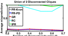
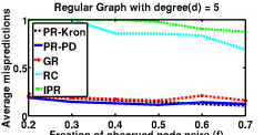
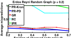
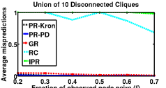
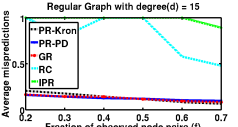
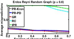
Figure 1: Synthetic Data: Average number of mispredictions ($er_{D}^{\ell^{0\text{-}1}}({\mathbf{f}})$, Eqn. (6)) vs fraction of sampled pairs $(f)$.

Generating ${\boldsymbol{\sigma}}_{n}^{*}$. For each of the above graphs, we compute ${\mathbf{f}}^{*}={\mathbf{A}}_{G}\boldsymbol{\alpha}$, where $\boldsymbol{\alpha}\in[0,1]^{n}$ is generated randomly, and set ${\boldsymbol{\sigma}}^{*}_{n}=\text{argsort}({\mathbf{f}}^{*})$ (see Pref-Rank, Step $3$ for definition).

All the performances are averaged across $10$ repeated runs. The results are reported in Fig. 1. In all the cases, our proposed algorithms PR-Kron and PR-PD outperforms the rest, with GR performing competitively well . As expected, RC and IPR perform very poorly as they could not exploit the underlying graph locality based ranking property.

6.2 Real-World Experiments

Datasets. We use $6$ standard real datasets for three graph learning tasks – $(a)$ Heart and Fourclass for BR, $(b)$ Vehicle and Vowel for OR, and $(c)$ House and Mg for FR.

Graph generation. For each dataset, we select $10$ random subsets of $40$ items each and construct a similarity matrix using RBF kernel, where $(i,j)^{\text{th}}$ entry is given by $\exp\big{(}\frac{-\|{\mathbf{x}}_{i}-{\mathbf{x}}_{j}\|^{2}}{2\mu^{2}}\big{)}$, ${\mathbf{x}}_{i}$ being the feature vector and $\mu$ the average distance. For each of the $10$ subsets, we constructed a graph by thresholding the similarity matrices about the mean.

Generating ${\boldsymbol{\sigma}}_{n}^{*}$. For each dataset, the provided item labels are used as the score vector ${\mathbf{f}}^{*}$ and we set ${\boldsymbol{\sigma}}^{*}_{n}=\text{argsort}({\mathbf{f}}^{*})$.

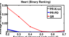
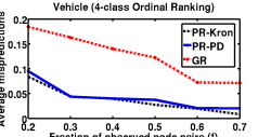
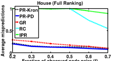
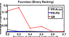
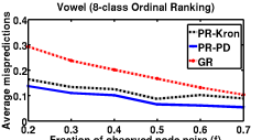
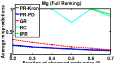
Figure 2: Real-World Data: Average number of mispredictions ($er_{D}^{\ell^{0\text{-}1}}({\mathbf{f}})$, Eqn. (6)) vs fraction of sampled pairs $(f)$.

For each of the task, the averaged result across $10$ randomly subsets are reported in Fig. 2. As before, our proposed methods PR-Kron and PR-PD perform the best, followed by GR. Once again RC and IPR perform poorly. Note that, the performance error increases from bipartite ranking (BR) to full ranking (FR), former being a relatively simpler task. Results on more datasets are available in App. E.2 and E.3.

7 Conclusion and Future Works

In this paper we addressed the problem of ranking nodes of a graph $G([n],E)$ given a random subsample of their pairwise preferences. Our proposed algorithm Pref-Rank, guarantees consistency with a required sample complexity of $O\big{(}n^{2}\chi(\bar{G})\big{)}^{\frac{2}{3}}$ – also gives novel insights by relating the ranking sample complexity with graph structural properties through chromatic number of $\bar{G}$, i.e. $\chi(\bar{G})$, for the first time. One possible future direction is to extend the setting to noisy preferences e.g. using BTL model Negahban et al. (2012), or analyse the problem with other measures of ranking losses e.g. NDCG, MAP Agarwal (2008). Furthermore, proving consistency of Pref-Rank algorithm using PD-Lab($G$) also remains an interesting direction to explore.

Appendix: How Many Preference Pairs Suffice to Rank a Graph Consistently?

Appendix A Discussion of Locality Property on RKHS

By definition, any smooth function ${\mathbf{f}}:V\mapsto{\mathbb{R}}$ over a graph $G(V,E)$ implies ${\mathbf{f}}$ to vary slowly on the neighbouring nodes of the graph $G$; i.e., if $(i,j)\in E$ then $f_{i}\approx f_{j},~{}\forall i,j\in V$. The standard way of defining this is by considering ${\mathbf{f}}^{\top}{\mathbf{L}}{\mathbf{f}}=\sum_{(i,j)\in E}(f_{i}-f_{j})^{2}$ to be small, say ${\mathbf{f}}^{\top}{\mathbf{L}}{\mathbf{f}}\leq B$, for some constant $B>0$. Clearly a small value of $B$ implies $|f_{i}-f_{j}|$ to be small for any two neighboring nodes, i.e. $(i,j)\in E$.

We first analyze the RKHS view of the above notion of smooth reward functions. Consider the SVD of the graph Laplacian ${\mathbf{L}}={\mathbf{Q}}{\boldsymbol{\Lambda}}{\mathbf{Q}}^{T}$, where ${\mathbf{Q}}=[{\mathbf{q}}_{1}~{}{\mathbf{q}}_{2}~{}\ldots~{}{\mathbf{q}}_{n}]\in{\mathbb{R}}^{n\times n}$, ${\boldsymbol{\Lambda}}=diag(\lambda_{1},\lambda_{2},\ldots,\lambda_{n})$ and suppose the singular values $\lambda_{i}=0,~{}\forall i>d$, for some $d\in[N]$. Now consider the linear space of real-valued vectors–

$${\mathcal{H}}(G)=\{{\mathbf{g}}\in{\mathbb{R}}^{n}\mid{\mathbf{g}}^{\top}{\mathbf{q}}_{i}=0~{}~{}\forall i>d\}$$

Note since ${\mathbf{L}}\in{\mathbf{S}}_{n}^{+}$ is positive semi-definite, the function $\|\cdot\|_{\mathbf{L}}:{\mathcal{H}}(G)\mapsto{\mathbb{R}}$, such that $\|{\mathbf{g}}\|_{\mathbf{L}}={\mathbf{g}}^{\top}{\mathbf{L}}{\mathbf{g}}$ defines a valid norm on ${\mathcal{H}}(G)$. In fact, one can show that ${\mathcal{H}}(G)$ along with the inner product $\langle\cdot,\cdot\rangle_{\mathbf{L}}:{\mathcal{H}}(G)\times{\mathcal{H}}(G)\mapsto{\mathbb{R}}$, such that $\langle{\mathbf{g}}_{1},{\mathbf{g}}_{2}\rangle_{\mathbf{L}}={\mathbf{g}}_{1}^{\top}{\mathbf{L}}{\mathbf{g}}_{2},~{}\forall{\mathbf{g}}_{1},{\mathbf{g}}_{2}\in{\mathcal{H}}(G)$, defines a valid RKHS with respect to the reproducing kernel ${\mathbf{K}}={\mathbf{L}}^{\dagger}$. This can be easily verified from the fact that $\forall{\mathbf{g}}\in{\mathcal{H}}(G)$, ${\mathbf{L}}^{\dagger}{\mathbf{L}}{\mathbf{g}}={\mathbf{g}}$, and hence $\langle{\mathbf{g}},{\mathbf{K}}_{i}\rangle_{{\mathbf{L}}}={\mathbf{g}}^{\top}{\mathbf{L}}{\mathbf{K}}{\mathbf{e}}_{i}=({\mathbf{L}}{\mathbf{K}}{\mathbf{g}})^{\top}{\mathbf{e}}_{i}=({\mathbf{L}}^{\dagger}{\mathbf{L}}{\mathbf{g}})^{\top}{\mathbf{e}}_{i}=g_{i},~{}\forall i\in[N]$.

Thus the smoothness assumption on the reward function ${\mathbf{f}}$, can alternatively be interpreted as ${\mathbf{f}}$ being small in terms of the RKHS norm $\|\cdot\|_{{\mathbf{L}}}$. The above interpretation gives us the insight of extending the notion of “smoothness” with respect to a general RKHS norm associated to some kernel matrix ${\mathbf{K}}\in{\mathbf{S}}_{n}^{+}$. More specifically, we choose the kernel matrix ${\mathbf{K}}$ from the set of orthonormal kernels ${\mathcal{K}}(G)$ and consider ${\mathbf{f}}$ to be smooth in the corresponding RKHS norm. Note here the Hilbert space of functions ${\mathcal{H}}({\mathbf{K}})$ is given by

$${\mathcal{H}}({\mathbf{K}})=\{{\mathbf{g}}\in{\mathbb{R}}^{n}\mid{\mathbf{g}}^{\top}{\mathbf{q}}_{i}=0~{}~{}\forall i>d\},$$ (7)

where same as before, the SVD of ${\mathbf{K}}={\mathbf{Q}}{\boldsymbol{\Lambda}}{\mathbf{Q}}^{\top}$, ${\mathbf{Q}}=[{\mathbf{q}}_{1},\ldots,{\mathbf{q}}_{n}]\in{\mathbb{R}}^{n\times n}$ being the orthogonal eigenvector matrix of ${\mathbf{K}}$, ${\boldsymbol{\Lambda}}=diag(\lambda_{1},\ldots\lambda_{n})$ be the diagonal matrix containing singular values of ${\mathbf{K}}$. Clearly $\lambda_{i}=0,~{}\forall i>d$ implies $r({\mathbf{K}})=d$. Also we define the corresponding inner product $\langle\cdot,\cdot\rangle_{\mathbf{K}}:{\mathcal{H}}({\mathbf{K}})\times{\mathcal{H}}({\mathbf{K}})\mapsto{\mathbb{R}}$, as $\langle{\mathbf{g}}_{1},{\mathbf{g}}_{2}\rangle_{\mathbf{K}}={\mathbf{g}}_{1}^{\top}{\mathbf{K}}^{\dagger}{\mathbf{g}}_{2},~{}\forall{\mathbf{g}}_{1},{\mathbf{g}}_{2}\in{\mathcal{H}}({\mathbf{K}})$. Then similarly as above, we can show that ${\mathcal{H}}({\mathbf{K}})$ along with $\langle\cdot,\cdot\rangle_{\mathbf{K}}$ defines a valid RKHS with respect to the reproducing kernel ${\mathbf{K}}$, as $\forall{\mathbf{g}}\in{\mathcal{H}}({\mathbf{K}})$, $\langle{\mathbf{g}},{\mathbf{K}}_{i}\rangle_{{\mathbf{K}}}={\mathbf{g}}^{\top}{\mathbf{K}}^{\dagger}{\mathbf{K}}{\mathbf{e}}_{i}=g_{i},~{}\forall i\in[n]$.

The RKHS norm $\|{\mathbf{g}}\|_{{\mathbf{K}}}={\mathbf{g}}^{\top}{\mathbf{K}}^{\dagger}{\mathbf{g}}$ defines a measure of the smoothness of ${\mathbf{g}}$, with respect to the kernel function ${\mathbf{K}}$. One way to see this is that $\forall{\mathbf{g}}\in{\mathcal{H}}({\mathbf{K}})$, $\|g_{i}-g_{j}\|=\|\langle{\mathbf{g}},({\mathbf{K}}(i,\cdot)-{\mathbf{K}}(j,\cdot))\rangle\|\leq\|{\mathbf{g}}\|_{{\mathbf{K}}}\|{\mathbf{K}}(i,\cdot)-{\mathbf{K}}(j,\cdot)\|_{\mathbf{K}}=\|{\mathbf{g}}\|_{{\mathbf{K}}}|(K_{ii}+K_{jj}-2K_{ij})|$, where the inequality follows from the Cauchy-Schwarz inequality of RKHS$({\mathbf{K}})$. Note since ${\mathbf{K}}\in{\mathcal{K}}(G)$, $K_{ii}=1,~{}\forall i\in[N]$, we have $|(K_{ii}+K_{jj}-2K_{ij})|\leq 4$ $\forall i,j\in[N]$. In particular, for two neighboring nodes $i$ and $j$ such that $(i,j)\in E$, it is expected that $K(i,j)\approx 1$ (i.e. ${\mathbf{u}}_{i}\approx{\mathbf{u}}_{j}$), in which case the quantity $|(K_{ii}+K_{jj}-2K_{ij})|\approx 0$. Thus to impose a smoothness constraint on ${\mathbf{g}}$, it is sufficient to upper bound $\|{\mathbf{g}}\|_{{\mathbf{K}}}\leq B$, for some fixed $B\in{\mathbb{R}}$, $\forall{\mathbf{g}}\in{\mathcal{H}}({\mathbf{K}})$.

We thus justify our assumption of $\|{\mathbf{f}}\|_{{\mathbf{K}}}\leq B$ which implies the ranking function (vector) ${\mathbf{f}}$ to be a smooth functions over the underlying graph $G$, with respect to embedding ${\mathbf{K}}$. Interestingly, ${\mathcal{H}}({\mathbf{K}})$ incorporates ${\mathcal{H}}(G)$ as its special case with ${\mathbf{K}}={\mathbf{L}}^{\dagger}$. Thus our space of ranking functions rightfully generalizes the Laplacian based rankings, as studied by Agarwal and Niyogi (2009); Agarwal (2010). From the definition of ${\mathcal{H}}({\mathbf{K}})$ in (7), it follows that the unknown ranking function ${\mathbf{f}}\in{\mathcal{H}}({\mathbf{K}})$, lies in the column space of ${\mathbf{K}}$, i.e. ${\mathbf{f}}={\mathbf{K}}\boldsymbol{\boldsymbol{\alpha}}$, for some $\boldsymbol{\boldsymbol{\tilde{\alpha}}}\in{\mathbb{R}}^{N}$. Also recall $\forall{\mathbf{K}}\in{\mathcal{K}}(G)$, there exists an ${\mathbf{U}}\in Lab(G)$, such that ${\mathbf{K}}={\mathbf{U}}^{\top}{\mathbf{U}}$, ${\mathbf{U}}\in{\mathbb{R}}^{N\times N}$. Thus we have ${\mathbf{f}}={\mathbf{K}}\boldsymbol{\boldsymbol{\alpha}}={\mathbf{U}}^{\top}{\mathbf{U}}\boldsymbol{\boldsymbol{\alpha}}={\mathbf{U}}^{\top}\boldsymbol{\tilde{\alpha}}$, where $\boldsymbol{\tilde{\alpha}}={\mathbf{U}}\boldsymbol{\alpha}$.

Lemma 14.

If ${\mathbf{f}}\in$ RKHS$({\mathbf{K}})$, ${\mathbf{f}}^{\top}{\mathbf{K}}{\mathbf{f}}\leq B$, and we define ${\mathbf{\tilde{K}}}={\mathbf{K}}\otimes{\mathbf{K}}$, $\tilde{\mathbf{f}}={\mathbf{f}}\otimes{\mathbf{f}}$, then $\tilde{\mathbf{f}}\in$ RKHS$({\mathbf{\tilde{K}}})$, $\tilde{\mathbf{f}}^{\top}{\mathbf{\tilde{K}}}\tilde{\mathbf{f}}\leq B^{2}$.

Proof.

The proof follows from the straightforward properties of tensor products. We describe it below from completeness: Since ${\mathbf{f}}\in\text{RKHS}({\mathbf{K}})$, we have ${\mathbf{f}}={\mathbf{K}}\boldsymbol{\alpha}$ for some $\boldsymbol{\alpha}\in{\mathbb{R}}^{n}$. Now

$$\tilde{\mathbf{f}} ={\mathbf{f}}\otimes{\mathbf{f}}=({\mathbf{K}}\boldsymbol{\alpha})\otimes({\mathbf{K}}\boldsymbol{\alpha})$$

$$=({\mathbf{K}}\otimes{\mathbf{K}})*(\boldsymbol{\alpha}\otimes\boldsymbol{\alpha})={\mathbf{\tilde{K}}}(\boldsymbol{\alpha}\otimes\boldsymbol{\alpha}),$$

and hence $\tilde{\mathbf{f}}\in$ RKHS$({\mathbf{\tilde{K}}})$, where the second last inequality follows due to the the properties of tensor product. Further more, using the same property, we have

$$\tilde{\mathbf{f}}^{\top}{\mathbf{K}}\tilde{\mathbf{f}} =({\mathbf{f}}\otimes{\mathbf{f}})^{\top}({\mathbf{K}}\otimes{\mathbf{K}})({\mathbf{f}}\otimes{\mathbf{f}})$$

$$=({\mathbf{f}}\otimes{\mathbf{f}})^{\top}({\mathbf{K}}{\mathbf{f}}\otimes{\mathbf{K}}{\mathbf{f}})$$

$$=({\mathbf{f}}^{\top}{\mathbf{K}}{\mathbf{f}})*({\mathbf{f}}^{\top}{\mathbf{K}}{\mathbf{f}})\leq B^{2}$$

∎

Definition 15.

Strong Product of Graphs. Given a graph $G=(V,E)$, strong product of $G$ with itself, denoted by $G\boxtimes G$, is defined over the vertex set $V(G\boxtimes G)=V\times V$, such that two nodes $(i,j),(i^{\prime},j^{\prime})\in V(G\boxtimes G)$ is adjacent in $G\boxtimes G$ if and only if $i=i^{\prime}$ and $(j,j^{\prime})\in E$, or $(i,i^{\prime})\in E$ and $j=j^{\prime}$, or $(i,i^{\prime})\in E$ and $(j,j^{\prime})\in E$. Note that for every node $k\in V(G\boxtimes G)$, there exists a corresponding node pair $(i_{k},j_{k})\in V\times V$ in the original graph $G$.

Let ${\mathbf{U}}=[{\mathbf{u}}_{1},\ldots,{\mathbf{u}}_{n}]\in{\mathbb{R}}^{d\times n}$ and $\mathbf{V}=[{\mathbf{v}}_{1},\ldots,{\mathbf{v}}_{n}]\in{\mathbb{R}}^{d^{\prime}\times n}$ be any two orthonormal representations of $G$. We denote ${\mathbf{u}}\otimes{\mathbf{v}}=[u_{1}v_{1}\ldots u_{1}v_{n}~{}u_{2}v_{1}\ldots u_{n}v_{n}]^{\top}\in{\mathbb{R}}^{dd^{\prime}}$ to be the kronecker (or outer) product of the two vectors ${\mathbf{u}}\in{\mathbb{R}}^{d},{\mathbf{v}}\in{\mathbb{R}}^{d^{\prime}}$. Let ${\mathbf{w}}_{k}={\mathbf{u}}_{i_{k}}\otimes{\mathbf{v}}_{j_{k}}\in{\mathbb{R}}^{dd^{\prime}}$, for every node $k\in V(G\boxtimes G)$. It is easy to see that any such embedding ${\mathbf{W}}=[{\mathbf{w}}_{1},{\mathbf{w}}_{2},\cdots{\mathbf{w}}_{n^{2}}]\in{\mathbb{R}}^{dd^{\prime}\times n^{2}}$ defines a valid orthonormal representation of $G\boxtimes G$. Using above, it can also be shown that $\vartheta(G\boxtimes G)=\vartheta^{2}(G)$ Lovász (1979).

Appendix B Appendix for Section 3.1

B.1 Proof of Theorem 3

See 3

Proof.

To proof the above result, let us first recall the error bound for learning classification models in transductive setting from El-Yaniv and Pechyony (2009).

Consider the problem of transductive binary classification over a fixed set $S_{m+u}=\{({\mathbf{x}}_{i},y_{i})\}_{i=1}^{m+u}$ of $m+u$ points, where ${\mathbf{x}}_{i}\in{\mathbb{R}}^{d}$ denotes the instances with their labels $y_{i}$. The learner is provided with the unlabeled (full) instance set $X_{m+u}=\{{\mathbf{x}}_{i}\}_{i=1}^{m+u}$. A set consisting of $m$ points is selected from $X_{m+u}$ uniformly at random among all subsets of size $m$. These $m$ points together with their labels are given to the learner as a training set. Renumbering the points, suppose the unlabeled training set points are denoted by $X_{m}=\{{\mathbf{x}}_{1},\ldots,{\mathbf{x}}_{m}\}$ and the labeled training set by $S_{m}=\{({\mathbf{x}}_{i},y_{i})\}_{i=1}^{m}$. The goal is to predict the labels of the unlabeled test points, $X_{u}=\{x_{m+1},\ldots,x_{m+u}\}=X_{m+u}\setminus X_{m}$, given $S_{m}\cup X_{u}$.

Consider any learning algorithm generates soft classification vectors ${\mathbf{h}}=(h_{1},\ldots,h_{m+u})\in{\mathbb{R}}^{m+u}$ (or equivalently ${\mathbf{h}}$ can also be seen as function such that $h:{\mathbf{X}}_{m+u}\mapsto{\mathbb{R}}$). $h_{i}(=h({\mathbf{x}}(i)))\in{\mathbb{R}}$ denotes the soft label for the example ${\mathbf{x}}_{i}$ given by the hypothesis ${\mathbf{h}}$. For actual (binary) classification of ${\mathbf{x}}_{i}$, the algorithm outputs $sgn(h_{i})$. The soft classification accuracy is measured with respect to the some loss function $\ell:\{\pm 1\}\times{\mathbb{R}}\mapsto[0,B]$. Thus $\ell(y_{i},h_{i})$ denotes the loss for the $i^{th}$ instance ${\mathbf{x}}_{i}$. We denote by $\ell^{0-1}$, the $0$-$1$ loss vector, i.e. $\ell^{0-1}(y_{i},h_{i})={\mathbf{1}}(y_{i}\neq sgn(h_{i}))$.

Theorem 16 (Transductive test error bound (Thm. 2) El-Yaniv and Pechyony (2009)).

Let ${\mathcal{H}}_{out}\subseteq{\mathbb{R}}_{m+u}$ denotes the set of all possible soft classification vectors generated by the learning algorithm, upon operating on all possible training/test set partitions, the loss function $\ell^{\rho}$ is $\rho$-lipschitz. Then for $c=\sqrt{\frac{32\ln(4e)}{3}}<5.05$, $Q=\big{(}\frac{1}{m}+\frac{1}{u}\big{)}$, and $S=\frac{m+u}{(m+u-1/2)(1-\frac{1}{2\max{(m,u)}})}$, and a fixed $\rho$, with probability of at least $(1-\delta)$ over the choice of the training set from $X_{m+u}$, for all $h\in{\mathcal{H}}_{out}$

$$\frac{1}{u}\sum_{i=m+1}^{m+u} \ell^{\rho}(y_{i},h_{i})\leq\frac{1}{m}\sum_{i=1}^{m}\ell^{\rho}(y_{i},h_{i})+\frac{R(H_{out})}{\rho}$$ (8)

$$+cBQ\sqrt{\min{(m,u)}}+B\sqrt{\frac{SQ}{2}\ln\frac{1}{\delta}},$$

where $R_{m+u}({\mathcal{H}}_{out})=Q{\mathbb{E}}_{{\boldsymbol{\gamma}}}\left[\sup_{{\mathbf{h}}\in{\mathcal{H}}_{out}}{\boldsymbol{\gamma}}^{\top}{\mathbf{h}}\right]$ is the pairwise Rademacher complexity of the function class ${\mathcal{H}}_{out}$, ${\boldsymbol{\gamma}}=(\gamma_{1},\ldots,\gamma_{m+u})$ be a vector of i.i.d. random variables such that $\gamma_{i}\in\{\pm 1,0\},~{}i\in[m+u]$, with probability $p$, $p$ and $1-2p$ respectively, with $p=\frac{mu}{(m+u)^{2}}$.

It is now straightforward to see that, for our current problem of interest training and test set sizes are respectively $m=Nf$ and $u=N(1-f)$. This immediately gives that $Q=\frac{1}{Nf(1-f)}$, $\min{(m,u)}=Nf$ and $p=f(1-f)$. The true labels of the pairwise classification problem are given by $y_{k}=sgn(\sigma^{*}(i_{k})-\sigma^{*}(j_{k})),~{}\forall k\in[N]$ and the function class ${\mathcal{H}}_{out}={\mathcal{H}}_{{\mathbf{\tilde{U}}}}$. Thus $R({\mathcal{H}}_{{\mathbf{\tilde{U}}}},{{\mathbf{\tilde{U}}}},p)=f(1-f)R({\mathcal{H}}_{out})$. Also note that for large $n$ and $f<\frac{1}{2}$, $S=\frac{N}{(N-1/2)\left(1-\frac{1}{N}\right)}\approx 1$. Thus (8) reduces to

$$er_{{\bar{S}}}^{\ell^{\rho}}[{\mathbf{f}}] =\frac{1}{u}\sum_{i=m+1}^{m+u}\ell^{\rho}(y_{i},h_{i})$$

$$\leq\frac{1}{m}\sum_{i=1}^{m}\ell^{\rho}(y_{i},h_{i})+\frac{R({\mathcal{H}}_{{\mathbf{\tilde{U}}}},{\mathbf{\tilde{U}}},p)}{\rho f(1-f)}$$

$$\quad\quad~{}~{}+\frac{C_{1}B}{(1-f)\sqrt{Nf}}\left(1+\sqrt{\ln\left(\frac{1}{\delta}\right)}\right),$$

for $C_{1}>0$ being the appropriate constant. Thus the claim follows. ∎

Appendix C Appendix for Section 4

C.1 Characterization: Choice of Optimal Embedding

In this section, we discuss different classes of pairwise preference graph embeddings and the corresponding generalization guarantees. We start by recalling Thm. $1$ of Ando and Zhang (2007), which provides a crucial characterization for the class of optimal embeddings:

Suppose ${\mathbf{f}}^{*}$ denotes the score function returned by the following optimization problem

$${\mathbf{f}}^{*}=\underset{{\mathbf{f}}\in{\mathbb{R}}^{N}}{\text{argmax}}~{}C^{\prime}{\mathbf{f}}^{\top}{\mathbf{\tilde{K}}}^{-1}{\mathbf{f}}+\hat{er}^{\ell^{\rho}}_{S_{m}}({\mathbf{f}}),$$

(note that for Pref-Rank  (Eqn. 3), $C^{\prime}=\frac{1}{2Cm}$ and $\ell^{\rho}=\ell^{hinge}$), then drawing a straightforward inference, we get

Corollary 17.

Suppose ${\mathbf{f}}^{*}$ denotes the optimal solution of (3). Then, over the random draw of $S_{m}\subseteq{\mathcal{P}}_{n}$, the expected generalization error w.r.t. any $\rho$-Lipschitz loss function $\ell^{\rho}$ is given by

$${\mathbb{E}}_{S_{m}}[er_{{\bar{S}}_{m}}^{\ell^{0-1}}({\mathbf{f}}^{*})]=\frac{1}{N-m}{\mathbb{E}}_{S_{m}}\left[\sum_{k=m+1}^{N}\ell^{0-1}(y_{k},{{\mathbf{f}}_{k}^{*}})\right]$$

$$\leq\inf_{{\mathbf{f}}\in{\mathbb{R}}^{N}}\frac{1}{c_{1}}\left[er_{S_{m}\cup{\bar{S}}_{m}}^{\ell^{\rho}}({\mathbf{f}})+C^{\prime}{\mathbf{f}}^{\top}{\mathbf{\tilde{K}}}^{-1}{\mathbf{f}}\right]+c_{2}\Bigg{(}\frac{tr_{p}({\mathbf{\tilde{K}}})}{\rho mC^{\prime}}\Bigg{)}^{p}$$

where $tr_{p}({\mathbf{\tilde{K}}})=\left(\frac{1}{N}\sum_{k=1}^{N}\tilde{K}_{kk}^{p}\right)^{\frac{1}{p}}$, $er_{S_{m}\cup{\bar{S}}_{m}}^{\ell^{\rho}}[{\mathbf{f}}]=\frac{1}{N}\sum_{k=1}^{N}\ell^{\rho}(y_{k},f_{k})$ and $p,c_{1},c_{2}>0$ are fixed constants dependent on $\ell^{\rho}$.

Now following a similar chain of arguments as in Ando and Zhang (2007), Cor. 17 implies that a normalized graph kernel ${\mathbf{\tilde{K}}}={\mathbf{\tilde{U}}}^{\top}{\mathbf{\tilde{U}}}$ such that $\tilde{K}_{kk}=1,\forall k\in[N]$ leads to improved generalization performance, since it ensures $tr({\mathbf{\tilde{K}}})_{p}$ to be constant. Furthermore, the following theorem shows that the class of ‘normalized’ graphs embeddings have high rademacher complexity.

C.2 Proof of Theorem 4

See 4

Proof.

Note that for any fixed realization of ${\boldsymbol{\gamma}}=[\gamma_{1},\ldots\gamma_{N}]$,

$$\sup_{{\mathbf{h}}\in{\mathcal{H}}_{{\mathbf{\tilde{U}}}}}\sum_{k=1}^{N}\gamma_{k}({\mathbf{h}}^{\top}{\mathbf{\tilde{u}}}_{k})=\sup_{{\mathbf{h}}\in{\mathcal{H}}_{{\mathbf{\tilde{U}}}}}{\mathbf{h}}^{\top}\big{(}{\mathbf{\tilde{U}}}{\boldsymbol{\gamma}}\big{)}$$

$$=\sup_{\boldsymbol{\beta}\in{\mathbb{R}}^{N}:\|\boldsymbol{\beta}\|_{\infty}\leq C}\boldsymbol{\beta}^{\top}{\mathbf{\tilde{U}}}^{\top}\big{(}{\mathbf{\tilde{U}}}{\boldsymbol{\gamma}}\big{)}$$

$$\leq\sup_{\boldsymbol{\beta}\in{\mathbb{R}}^{N}:\|\boldsymbol{\beta}\|_{\infty}\leq C}\|{\mathbf{\tilde{U}}}\boldsymbol{\beta}\|_{2}\|{\mathbf{\tilde{K}}}{\boldsymbol{\gamma}}\|_{2}~{}~{}\big{(}\mbox{Cauchy-Schwarz Ineq.}\big{)}$$

$$\leq\sqrt{\lambda_{1}({\mathbf{\tilde{K}}})}\sup_{\boldsymbol{\beta}\in{\mathbb{R}}^{N}:\|\boldsymbol{\beta}\|_{\infty}\leq C}\|\boldsymbol{\beta}\|_{2}\|{\mathbf{\tilde{U}}}{\boldsymbol{\gamma}}\|_{2}$$

$$\leq C\sqrt{N\lambda_{1}({\mathbf{\tilde{K}}})}\|{\mathbf{\tilde{U}}}{\boldsymbol{\gamma}}\|_{2}$$

Using above we further get:

$$R({\mathcal{H}}_{{\mathbf{\tilde{U}}}},{\mathbf{\tilde{U}}},p)\leq\frac{1}{N}{\mathbb{E}}_{{\boldsymbol{\gamma}}}\left[C\sqrt{N\lambda_{1}({\mathbf{\tilde{K}}})}\|U{\boldsymbol{\gamma}}\|_{2}\right]$$

$$=\frac{C\sqrt{\lambda_{1}({\mathbf{\tilde{K}}})}}{\sqrt{N}}{\mathbb{E}}_{{\boldsymbol{\gamma}}}\left[\sqrt{{{\boldsymbol{\gamma}}^{\top}{\mathbf{\tilde{K}}}{\boldsymbol{\gamma}}}}\right]$$

$$\leq\frac{C\sqrt{\lambda_{1}({\mathbf{\tilde{K}}})}}{\sqrt{N}}\sqrt{{\mathbb{E}}_{{\boldsymbol{\gamma}}}\left[{\boldsymbol{\gamma}}^{\top}{\mathbf{\tilde{K}}}{\boldsymbol{\gamma}}\right]}~{}~{}\big{(}\mbox{Jensen's Inequality}\big{)}$$

$$=\frac{C\sqrt{\lambda_{1}({\mathbf{\tilde{K}}})}}{\sqrt{N}}\sqrt{2p(tr({\mathbf{\tilde{K}}}))}=\frac{C}{\sqrt{N}}\sqrt{2p\lambda_{1}({\mathbf{\tilde{K}}})(tr({\mathbf{\tilde{K}}}))},$$

where the second last equality follows from the fact that ${\mathbb{E}}_{{\boldsymbol{\gamma}}}\left[{\boldsymbol{\gamma}}^{\top}{\mathbf{\tilde{K}}}{\boldsymbol{\gamma}}\right]=2p\sum_{k=1}^{N}\tilde{K}_{kk}=2p(tr({\mathbf{\tilde{K}}}))$, as ${\boldsymbol{\gamma}}=(\gamma_{1},\ldots,\gamma_{N})$ be a vector of i.i.d. random variables such that $\gamma_{i}\in\{+1,-1,0\},~{}i\in[N]$, with probability $p$, $p$ and $1-2p$ respectively and $tr({\mathbf{\tilde{K}}})=\sum_{k=1}^{N}\tilde{K}_{kk}$. The proof now follows from the fact that $tr({\mathbf{\tilde{K}}})=N$, since $\tilde{K}_{kk}=1,~{}\forall k\in[N]$.

∎

C.3 Proof of Lemma 5

See 5

Proof.

To show this, we first proof the following lemmas.

Lemma 18.

Let ${\mathbf{\tilde{U}}}_{P}=[\mathbf{\tilde{u}}_{ij}]_{(i,j)\in{\mathcal{P}}_{n}}\in{\mathbb{R}}^{d^{2}\times N}$ be the embedding matrix only for the node-pairs in ${\mathcal{P}}_{n}$. ${\mathbf{\tilde{K}}}_{P}={\mathbf{\tilde{U}}}_{P}^{\top}{\mathbf{\tilde{U}}}_{P},\,{\mathbf{\tilde{K}}}={\mathbf{\tilde{U}}}^{\top}{\mathbf{\tilde{U}}}$. Then $\lambda_{1}({\mathbf{\tilde{K}}}_{P})\leq\lambda_{1}({\mathbf{\tilde{K}}})$.

Proof.

We have that $\lambda_{1}({\mathbf{\tilde{K}}}_{P})=\sup_{{\mathbf{x}}\in{\mathbb{R}}^{N}}\frac{{\mathbf{x}}^{\top}{\mathbf{\tilde{K}}}_{P}{\mathbf{x}}}{\|{\mathbf{x}}\|_{2}^{2}}$. Let ${\mathbf{x}}_{1}=\underset{{\mathbf{x}}\in{\mathbb{R}}^{N}}{\text{argsup}}\frac{{\mathbf{x}}^{\top}{\mathbf{\tilde{K}}}_{P}{\mathbf{x}}}{\|{\mathbf{x}}\|_{2}^{2}}$.

Note that ${\mathbf{\tilde{U}}}=[{\mathbf{\tilde{U}}}_{1},{\mathbf{\tilde{U}}}_{2},\ldots,{\mathbf{\tilde{U}}}_{n^{2}}]\in{\mathbb{R}}^{d^{2}\times n^{2}}$, and ${\mathbf{\tilde{U}}}_{P}=[{\mathbf{\tilde{U}}}_{P_{1}},{\mathbf{\tilde{U}}}_{P_{2}},\ldots,{\mathbf{\tilde{U}}}_{P_{N}}]\in{\mathbb{R}}^{d^{2}\times N}$, where $\mathbf{\tilde{u}}_{k}={\mathbf{u}}_{i_{k}}\circ{\mathbf{u}}_{j_{k}},\,\forall(i_{k},j_{k})\in[n]\times[n]$ and ${(\mathbf{\tilde{u}}_{P})}_{k}={\mathbf{u}}_{i_{k}}\circ{\mathbf{u}}_{j_{k}},\,\forall(i_{k},j_{k})\in{\mathcal{P}}_{n}$.

Let us define $k^{\prime}(i,j)=n(i-1)+j,~{}\forall(i,j)\in[n]\times[n]$ and $k(i,j)=\sum_{l=1}^{i-1}(n-l)+(j-i),~{}~{}\forall(i,j)\in{\mathcal{P}}_{n}$.

Clearly ${\mathbf{\tilde{K}}}(k^{\prime}(i,j),k^{\prime}(u,v))={\mathbf{\tilde{K}}}_{P}(k(i,j),k(u,v))$, $\forall(i,j),(u,v)\in{\mathcal{P}}_{n}$ such that Now let us consider ${\mathbf{\tilde{x}}}_{1}\in{\mathbb{R}}^{n^{2}}$ such that

$${\mathbf{\tilde{x}}}_{1}(k^{\prime}(i,j))=\begin{cases}{\mathbf{x}}_{1}(k(i,j)),\,\forall(i,j)\in{\mathcal{P}}_{n},\\ 0,\text{ otherwise}\end{cases}$$

Note that this implies $\lambda_{1}({\mathbf{\tilde{K}}})=\sup_{{\mathbf{\tilde{x}}}\in{\mathbb{R}}^{n^{2}}}\frac{{\mathbf{\tilde{x}}}^{\top}{\mathbf{\tilde{K}}}{\mathbf{\tilde{x}}}}{\|{\mathbf{\tilde{x}}}\|_{2}^{2}}\geq\frac{{\mathbf{\tilde{x}}}_{1}^{\top}{\mathbf{\tilde{K}}}{\mathbf{\tilde{x}}}_{1}}{\|{\mathbf{\tilde{x}}}_{1}\|_{2}^{2}}=\frac{{\mathbf{x}}_{1}^{\top}{\mathbf{\tilde{K}}}_{P}{\mathbf{x}}_{1}}{\|{\mathbf{x}}_{1}\|_{2}^{2}}=\lambda_{1}({\mathbf{\tilde{K}}}_{P})$, proving the claim. ∎

Lemma 19.

Let ${\mathbf{\tilde{K}}}={\mathbf{\tilde{U}}}^{\top}{\mathbf{\tilde{U}}},\,{\mathbf{K}}={\mathbf{U}}^{\top}{\mathbf{U}}$, for any ${\mathbf{\tilde{U}}}\in\text{SP-Lab}(G)$, and the corresponding ${\mathbf{U}}\in\text{Lab}(G)$. Then $\lambda_{1}({\mathbf{\tilde{K}}})=(\lambda_{1}({\mathbf{K}}))^{2}$.

Proof.

Note that $\lambda_{1}({\mathbf{K}})=\sup_{{\mathbf{x}}\in{\mathbb{R}}^{n}}\frac{{\mathbf{x}}^{\top}{\mathbf{K}}{\mathbf{x}}}{\|{\mathbf{x}}\|_{2}^{2}}$. Let ${\mathbf{x}}_{1}=\text{argsup}_{{\mathbf{x}}\in{\mathbb{R}}^{n}}\frac{{\mathbf{x}}^{\top}{\mathbf{K}}{\mathbf{x}}}{\|{\mathbf{x}}\|_{2}^{2}}$.

The crucial observation is that

$${\mathbf{\tilde{K}}}={\mathbf{K}}\circ{\mathbf{K}}=\begin{bmatrix}K_{11}{\mathbf{K}}&\cdots&K_{1n}{\mathbf{K}}\\ .&.&.\\ .&.&.\\ .&.&.\\ K_{n1}{\mathbf{K}}&\cdots&K_{nn}{\mathbf{K}}\\ \end{bmatrix}.$$

Let us define ${\mathbf{\tilde{x}}}_{1}={\mathbf{x}}_{1}\circ{\mathbf{x}}_{1}\in{\mathbb{R}}^{n^{2}}$. Note that $\|{\mathbf{\tilde{x}}}\|_{2}=\|{\mathbf{x}}\|_{2}^{2}$. Then $\lambda_{1}({\mathbf{\tilde{K}}})=\sup_{{\mathbf{\tilde{x}}}\in{\mathbb{R}}^{n^{2}}}\frac{{\mathbf{\tilde{x}}}^{\top}{\mathbf{\tilde{K}}}{\mathbf{\tilde{x}}}}{\|{\mathbf{\tilde{x}}}\|_{2}^{2}}=\frac{{\mathbf{\tilde{x}}}_{1}^{\top}{\mathbf{\tilde{K}}}{\mathbf{\tilde{x}}}_{1}}{\|{\mathbf{\tilde{x}}}_{1}\|_{2}^{2}}=\frac{\big{(}{\mathbf{x}}_{1}^{\top}{\mathbf{K}}{\mathbf{x}}_{1}\big{)}^{2}}{\|{\mathbf{x}}_{1}\|_{2}^{4}}=(\lambda_{1}({\mathbf{K}}))^{2}$. ∎

Thus applying Lem. 18 and 19, we get, $\lambda_{1}({\mathbf{\tilde{K}}}_{P})\leq\lambda_{1}({\mathbf{\tilde{K}}})=(\lambda_{1}({\mathbf{K}}))^{2}$. The proof of Lem. 5 now follows from Thm. 4.

∎

C.4 Proof of Theorem 6

See 6

The proof follows by applying Lem. 5 to Thm. 3 for $p=f(1-f)$.

C.5 Proof of Lemma 7

See 7

Proof.

Let ${\mathbb{E}}=[{\mathbf{e}}_{i}-{\mathbf{e}}_{j}]_{(i,j)\in{\mathcal{P}}_{n}}\in\{0,\pm 1\}^{n\times N}$, where ${\mathbf{e}}_{i}$ denotes the $i^{th}$ standard basis of ${\mathbb{R}}^{n}$, $\forall i\in[n]$. We start by proving the following lemma:

Lemma 20.

If ${\mathbf{U}}\in Lab(G)$, ${\mathbf{K}}={\mathbf{U}}^{\top}{\mathbf{U}}$, ${\mathbf{\tilde{U}}}={\mathbf{U}}{\mathbb{E}}\in$ PD-Lab($G$)  and ${\mathbf{\tilde{K}}}={\mathbf{\tilde{U}}}^{\top}{\mathbf{\tilde{U}}}$, then $\lambda_{1}({\mathbf{\tilde{K}}})=2n\lambda_{1}({\mathbf{K}})$.

Proof.

By definition of $\lambda_{1}({\mathbf{\tilde{K}}})$, we know that

$$\lambda_{1}({\mathbf{\tilde{K}}}) =\sup_{{\mathbf{x}}\in{\mathbb{R}}^{n}}\frac{{\mathbf{x}}^{\top}{\mathbf{\tilde{K}}}{\mathbf{x}}}{\|{\mathbf{x}}\|_{2}^{2}}$$

$$=\sup_{{\mathbf{x}}\in{\mathbb{R}}^{N}}\frac{{\mathbf{x}}^{\top}{\mathbb{E}}^{\top}{\mathbf{K}}{\mathbb{E}}{\mathbf{x}}}{\|{\mathbf{x}}\|_{2}^{2}}$$

$$=\sup_{{\mathbf{x}}\in{\mathbb{R}}^{N}}\frac{({\mathbb{E}}{\mathbf{x}})^{\top}{\mathbf{K}}({\mathbb{E}}{\mathbf{x}})}{\|{\mathbf{x}}\|_{2}^{2}}$$

$$=\sup_{{\mathbf{x}}\in{\mathbb{R}}^{N}}\frac{\lambda_{{\mathbf{K}}}\|{\mathbb{E}}{\mathbf{x}}\|_{2}^{2}}{\|{\mathbf{x}}\|_{2}^{2}}$$

$$\leq 2n\lambda_{{\mathbf{K}}},$$

where the last inequality follows from the fact that, for any ${\mathbf{x}}\in{\mathbb{R}}^{N}$, $\|{\mathbb{E}}{\mathbf{x}}\|_{2}^{2}\leq 2n\|{\mathbf{x}}\|_{2}^{2}$. ∎

Now further applying Thm. 4 for ${\mathbf{\tilde{U}}}\in$ PD-Lab($G$), we get $R({\mathcal{H}}_{{\mathbf{\tilde{U}}}},{\mathbf{\tilde{U}}},p)\leq C\sqrt{2p\lambda_{1}({\mathbf{\tilde{K}}})}\leq C\sqrt{2p\lambda_{1}({\mathbf{\tilde{K}}})}$, since $tr({\mathbf{\tilde{K}}})\leq N$ and the result now follows from Lem. 20. ∎

C.6 Proof of Theorem 8

See 8

Proof.

The proof follows by applying Lem. 7 to Thm. 3 for $p=f(1-f)$. ∎

C.7 Proof of Lemma 9

See 9

Proof.

For $G(n,q)$ graphs, Füredi and Komlós (1981) showed that with high probability $1-e^{-\sqrt{n}}$, $\lambda_{1}({\mathbf{A}}_{G})=nq(1+o(1))$ and $|\lambda_{n}({\mathbf{A}}_{G})|\leq 2\sqrt{nq(1-q)}$. As $q=O(1)$, note that $\lambda_{1}({\mathbf{A}}_{G})=\Theta(n)$ and $\lambda_{n}({\mathbf{A}}_{G})=\Theta(\sqrt{n})$. Thus, choosing $\tau=\Theta(\sqrt{n})$ makes ${\mathbf{K}}_{LS}(G)$ a positive semi-definite matrix, and clearly $\lambda_{1}({\mathbf{K}}_{LS}(G))=\Theta(\sqrt{n})$. Moreover since ${\mathbf{\tilde{K}}}_{LS}={\mathbf{K}}_{LS}\otimes{\mathbf{K}}_{LS}$, we have $\lambda_{1}({\mathbf{\tilde{K}}}_{LS})=\big{(}\lambda_{1}({\mathbf{K}}_{LS})\big{)}^{2}$, as follows from Lem. 19). The claim now follows from Thm. 4 and Lem. 18.

∎

C.8 Embedding with graph Laplacian.

The popular choice of graph kernel uses the inverse of the Laplacian matrix. Formally, let $d_{i}$ denotes the degree of vertex $i\in[n]$ in graph $G$, $d_{i}={({\mathbf{A}}_{G})}_{i}^{\top}{\mathbf{1}}_{n}$, and ${\mathbf{D}}$ denote a diagonal matrix such that $D_{ii}=d_{i},\forall i\in[n]$. Then the Laplacian and normalized Laplacian kernel of $G$ is defined as follows:

$${\mathbf{K}}_{Lap}(G)=({\mathbf{D}}-{\mathbf{A}}_{G})^{\dagger}\text{ and}$$

$${\mathbf{K}}_{nLap}(G)=({\mathbf{I}}_{n}-{\mathbf{D}}^{-1/2}{\mathbf{A}}_{G}{\mathbf{D}}^{-1/2})^{\dagger}.$$

Simlar to LS-labelling, one could define the embedding of $G\boxtimes G$ using Kron-Lab($G\boxtimes G$) or PD-Lab($G$) with ${\mathbf{K}}_{Lap}$ and ${\mathbf{K}}_{nLap}$. However, we observe that the Rademahcer complexity of function associated with Laplacian is an order magnitude smaller than that of LS-labelling for graphs with high connectivity – we summarize our findings in Table 2. Experimental results in Section 6 illustrate our observation.

Graph	Laplacian	LS-labelling
Complete graph $K_{n}$	$\Theta(1)$	$\Theta(n)$
Random Graphs $G(n,1/2)$	$\Theta(1)$	$\Theta(\sqrt{n})$
Complete Bipartite	$\Theta(1)$	$\Theta(1)$
Star $S_{n}$	$\Theta(1)$	$\Theta(1)$

Table 2: Rademacher complexity measure of Laplacian and LS-labelling graph embeddings (assuming $C,p=O(1)$).

Appendix D Appendix for Section 5

D.1 Proof of Theorem 10

See 10

Proof.

We first bound the total number of pairwise mispredictions of $f$, given by $N{er}^{\ell^{0-1}}_{n}[{\mathbf{f}}]$. Note that $N{er}^{\ell^{0-1}}_{n}[{\mathbf{f}}]\leq N{er}^{\ell^{ramp}}_{n}[{\mathbf{f}}]$. (see Sec. 2.1 for definitions of $\ell^{0-1}_{n}[{\mathbf{f}}]$ and $\ell^{ramp}_{n}[{\mathbf{f}}]$).

Now applying Cor. 6 for ramp loss $\ell^{ramp}$ with $\delta=\frac{1}{n}$, we get that with probability atleast $(1-\frac{1}{N})$,

$$Ner_{n}^{\ell^{ramp}}[{\mathbf{f}}]=\sum_{k=1}^{N}\ell^{ramp}(y_{k},f_{k})$$

$$=\left(\sum_{k=Nf+1}^{N}\ell^{ramp}(y_{k},f_{k})+\sum_{k=1}^{Nf}\ell^{ramp}(y_{k},f_{k})\right)$$

$$=\left((N-Nf){er}^{l^{ramp}}_{{\bar{S}}}[{\mathbf{f}}]+Nf{er}^{l^{ramp}}_{S}[{\mathbf{f}}]\right)$$

$$\leq\Bigg{(}(N(1-f)+Nf){er}^{l^{ramp}}_{S}[{\mathbf{f}}]$$

$$\qquad+\frac{N\sqrt{2(1-f)}C\lambda_{1}({\mathbf{K}})}{\rho\sqrt{f}}+\frac{C_{1}NB\sqrt{\ln N}}{\sqrt{Nf}}\Bigg{)}$$

$$\qquad\qquad\qquad\qquad\qquad\qquad\qquad~{}(\text{ from Thm. }\ref{cor:rad})$$

$$=N\Bigg{(}er_{S}^{\ell^{ramp}}[{\mathbf{f}}]+\frac{C\lambda_{1}({\mathbf{K}})\sqrt{2(1-f)}}{\sqrt{f}}+\frac{C_{1}\sqrt{2\ln n}}{\sqrt{Nf}}\Bigg{)},$$

$$\leq N\Bigg{(}er_{S}^{\ell^{hinge}}[{\mathbf{f}}]+\frac{C\lambda_{1}({\mathbf{K}})\sqrt{2(1-f)}}{\sqrt{f}}+\frac{C_{1}\sqrt{2\ln n}}{\sqrt{Nf}}\Bigg{)}$$

where the second last inequality is because for ramp loss, $\rho$ and $B$ both are $1$. The last equality follows from the fact that hinge loss is an upper bound of the ramp loss.

Let us define ${\mathbf{\tilde{U}}}_{P}=[\mathbf{\tilde{u}}_{ij}]_{(i,j)\in{\mathcal{P}}_{n}}\in{\mathbb{R}}^{d^{2}\times N}$ to be the embedding matrix only for the node-pairs in ${\mathcal{P}}_{n}$. ${\mathbf{\tilde{K}}}_{P}={\mathbf{\tilde{U}}}_{P}^{\top}{\mathbf{\tilde{U}}}_{P}$. Also let us define

$$\text{PSP-Lab}(G\boxtimes G) =\{{\mathbf{\tilde{U}}}_{P}\in{\mathbb{R}}^{d^{2}\times N}\mid{\mathbf{U}}\in\mbox{Lab}(G)\}.$$

The key of the proof lies in the following derivation that maps $\vartheta(G)$ to the training set error $er_{S}^{\ell^{hinge}}[{\mathbf{f}}]$. Specifically, note that:

$$2C(Nf)er_{S}^{\ell^{hinge}}[{\mathbf{f}}]=2C\sum_{i=1}^{Nf}\ell^{hinge}(y_{k},f_{k})$$

$$\leq\min_{{\mathbf{\tilde{U}}}\in\mbox{PSP-Lab}(G\boxtimes G),\|{\mathbf{c}}\|_{2}=1}\max_{k=1}^{N}\frac{1}{(c^{\top}{\mathbf{\tilde{U}}}_{k})^{2}}$$

$$\leq\min_{{\mathbf{\tilde{U}}}\in\text{Kron-Lab($G\boxtimes G$)},\|{\mathbf{c}}\|_{2}=1}\max_{k=1}^{n^{2}}\frac{1}{(c^{\top}{\mathbf{\tilde{U}}}_{k})^{2}}$$

$$=\min_{{\mathbf{\tilde{U}}}\in\mbox{Lab}(G\boxtimes G),\|{\mathbf{c}}\|_{2}=1}\max_{k=1}^{n^{2}}\frac{1}{(c^{\top}{\mathbf{\tilde{U}}}_{k})^{2}}$$

$$={\vartheta(G\boxtimes G)}$$

$$={(\vartheta(G))^{2}},$$ (9)

where the first inequality follows from a similar derivation as given in Thm. $5.2$ of Shivanna and Bhattacharyya (2014) which relates optimum SVM objective to Lóvasz-$\vartheta$. The second inequality is obvious as PSP-Lab$(G\boxtimes G)\subset$ Kron-Lab($G\boxtimes G$). Thus we get that $er_{S}^{\ell^{hinge}}[f]=\frac{(\vartheta(G))^{2}}{2CNf}$. Combining everything we now have:

$$er_{n}^{\ell^{0-1}}[{\mathbf{f}}]\leq er_{n}^{\ell^{ramp}}[f]=\frac{1}{N}\sum_{k=1}^{N}\ell^{ramp}(y_{k},f_{k})$$

$$\leq\Bigg{(}\frac{\vartheta(G_{n})^{2}}{2CNf}+\frac{C\lambda_{1}({\mathbf{K}})\sqrt{2(1-f)}}{\sqrt{f}}+\frac{C_{1}\sqrt{2\ln n}}{\sqrt{Nf}}\Bigg{)}$$

$$\leq\Bigg{(}\frac{\vartheta(G_{n})^{2}}{2CNf}+\frac{Cn\sqrt{2(1-f)}}{\vartheta(G)\sqrt{f}}+\frac{C_{1}\sqrt{2\ln n}}{\sqrt{Nf}}\Bigg{)}$$

Where the last inequality follows from $\lambda_{1}({\mathbf{K}})\leq\vartheta(\bar{G}_{n})$, $\vartheta({G}_{n})\vartheta(\bar{G}_{n})=n$ Lovász (1979). Further optimizing over $C$ we get that at $C^{*}=\bigg{(}\frac{\vartheta(G_{n})^{3}}{Nn\sqrt{8f(1-f)}}\bigg{)}^{\frac{1}{2}}$, using which we get

$$er_{n}^{\ell^{0-1}}[{\mathbf{f}}]=\frac{1}{N}\sum_{k=1}^{N}\ell^{0-1}(y_{k},h_{k})$$

$$\leq\Bigg{(}2\bigg{(}\frac{\vartheta(G_{n})}{(n-1)f}\sqrt{\frac{2(1-f)}{f}}\bigg{)}^{\frac{1}{2}}+\frac{C_{1}\sqrt{2\ln n}}{\sqrt{Nf}}\Bigg{)}$$

Above proves the first half of the result. The second result immediately follows from above with the additional observation that $d_{k}(\sigma^{*},{\hat{\sigma}})\leq 3er_{n}^{\ell^{0-1}}[{\mathbf{f}}]$ and and the fact that

$$d_{s}({\boldsymbol{\sigma}}_{1},{\boldsymbol{\sigma}}_{2})\leq 2d_{k}({\boldsymbol{\sigma}}_{1},{\boldsymbol{\sigma}}_{2})$$ (10)

where $d$ being the Kendall’s tau $(d_{k})$ or Spearman’s footrule $(d_{s})$ ranking loss, which concludes the proof. ∎

Proof of Lemma 11 See 11

Proof.

From Thm. 10 we have that there exists a constant positive $C_{0}>0$ and an positive integer $n_{0}\in{\mathbb{N}}$ such that $\forall n\geq n_{0}$

$$d({\boldsymbol{\sigma}}^{*}_{n},\boldsymbol{\hat{\sigma}}_{n}) \leq C_{0}\Bigg{(}\bigg{(}\frac{\vartheta(G_{n})}{nf}\sqrt{\frac{(1-f)}{f}}\bigg{)}^{\frac{1}{2}}+\frac{C_{1}\sqrt{2\ln n}}{\sqrt{Nf}}\Bigg{)}$$

$$\leq C_{0}\Bigg{(}\frac{1}{f^{\frac{3}{4}}}\sqrt{\bigg{(}\frac{\vartheta(G_{n})}{n}\bigg{)}}+\frac{C_{1}\sqrt{2\ln n}}{\sqrt{Nf}}\Bigg{)}$$ (11)

Now that if $\vartheta(G_{n})=o(n^{c})$ for some $c\in[0,1)$ (recall $\vartheta(G_{n})\in[1,n]$) and if we choose $\varepsilon\leq\frac{(1-c)}{2}$ this makes $f^{*}=\bigg{(}\frac{\sqrt{\vartheta(G_{n})}}{n^{\frac{1}{2}-\varepsilon}}\bigg{)}^{\frac{4}{3}}$ to be a valid assignment as that ensures $f^{*}\in[0,1]$. Furthermore, (D.1) suggests that observing only $f^{*}$ fraction of nodes would suffice to achieve ranking consistency since that implies $d({\boldsymbol{\sigma}}^{*}_{n},\boldsymbol{\hat{\sigma}}_{n})=O(\frac{1}{n^{\varepsilon}})\to 0$, as $n\to\infty$. ∎

Proof of Theorem 12

See 12

Proof.

From Lemma 11, using $f^{*}$ fraction of nodes immediately leads to the sample complexity:

$$Nf^{*}\leq\frac{n^{2}}{2}\bigg{(}\frac{{\vartheta(G_{n})}}{n^{1-2\varepsilon}}\bigg{)}^{\frac{2}{3}}=\frac{1}{2}(n^{2+2\varepsilon}\vartheta(G_{n}))^{\frac{2}{3}}$$

The result now follows from Lem. 11 and Lovász sandwich theorem: $\vartheta(G)\leq\chi(\bar{G})$ for any graph $G$ Lovász (1979). ∎

Proof of Corollary 13

See 13

Proof.

The result follows from the proof of Theorem 12 upon by substituting the values of $\vartheta(G)$ or $\chi(\bar{G})$ (note $\vartheta(G)\leq\chi(\bar{G})$) in the corresponding graphs as given below:

1. Complete graphs: $\chi(\bar{G})=1$

2. Union of $k$ disjoint cliques: $\chi(\bar{G})=k$

3. Complement of Power-law graphs: $\vartheta(\bar{G})=\Theta(\sqrt{n})$ Shivanna and Bhattacharyya (2014); Frieze et al. (2007)

4. Random graphs: $\vartheta(G)=\Theta(\sqrt{n})$, with high probability Coja-Oghlan (2005).

5. Complement of $k$-colorable graphs: $\chi(\bar{G})=k$.

∎

Appendix E Additional Experiments

E.1 Additional Results: Experiments of Synthetic Datasets

Plots comparing only PR-Kron, PR-PD, and GR

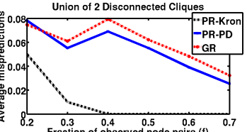
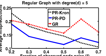
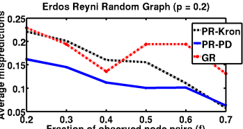
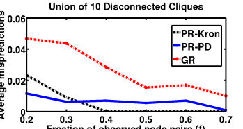
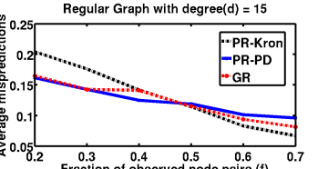
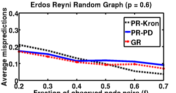
Figure 3: Synthetic Data: Average number of misprediction ($er_{D}^{\ell^{0\text{-}1}}({\mathbf{f}})$, Eqn. 6) vs fraction of sampled pairs$(f)$

More Synthetic Experiments

We consider a $G(n,p,q)$ random graph with $n=100$ nodes, $p=0.6,q=0.1$, where nodes $[1$-$50]$ and $[51$-$100]$ are densely clustered, and nodes within the same cluster are connected with edge probability $p$ and that of two different clusters are connected with probability $q$. We also consider the nodes within same cluster to be closer in terms of their preference scores. More specifically, for the task of full ranking, we randomly assign a permutation to the 100 nodes such that all nodes in cluster 1 are ranked above all nodes in cluster 2 (below 50 and all nodes $(51$-$100)$ are ranked above 50). Similarly for ordinal ranking we randomly assign a rating from $1-10$ to each graph node such that all nodes in cluster 1 are rated higher than that of cluster 2. Finally for Bipartite ranking, we randomly assign a (0,1) binary label to each node such that nodes in cluster one are $80\%$ more likely to score higher than that of cluster 2. For each of the three tasks, we repeat the experiment for $10$ times and compare the averaged performances of PR-Kron with GR. Table 3 shows that on an average Pref-Rank  with Kron-Lab($G\boxtimes G$)  performs better than Graph Rank  for all three tasks.

Task	PR-Kron (in %)	GR (in %)
BR	07.5	08.2
OR(10)	12.3	17.6
FR	11.8	18.6

Table 3: Synthetic data: Average number of mispredictions.

E.2 Additonal Results: Experiments of Real Datasets

Plots comparing only PR-Kron, PR-PD, and GR

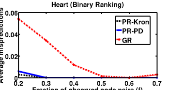
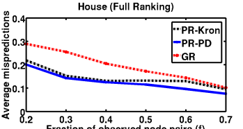
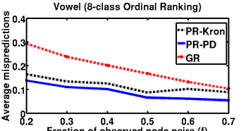
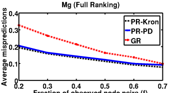
Figure 4: Real Data: Average number of misprediction ($er_{D}^{\ell^{0\text{-}1}}({\mathbf{f}})$, Eqn. 6) vs fraction of sampled pairs$(f)$

E.3 More Experiments on Real Datasets

Datasets. $a$. Ionosphere and Diabetes for BR $b$. Bodyfat for FR.

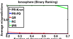
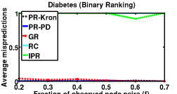
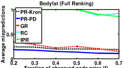
Figure 5: Real Data: Average number of misprediction ($er_{D}^{\ell^{0\text{-}1}}({\mathbf{f}})$, Eqn. 6) vs fraction of sampled pairs$(f)$

Plots comparing only PR-Kron, PR-PD, and GR

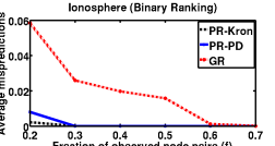
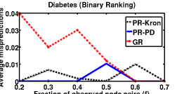
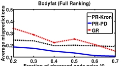
Figure 6: Real Data: Average number of misprediction ($er_{D}^{\ell^{0\text{-}1}}({\mathbf{f}})$, Eqn. 6) vs fraction of sampled pairs$(f)$

References

- Agarwal and Chakrabarti [2007] Alekh Agarwal and Soumen Chakrabarti. Learning Random Walks to Rank Nodes in Graphs. In Proceedings of the 24th international conference on Machine learning, pages 9–16. ACM, 2007.
- Agarwal [2008] Shivani Agarwal. Transductive Ranking on Graphs. Tech Report, 2008.
- Agarwal [2010] Shivani Agarwal. Learning to Rank on Graphs. Machine learning, 81(3):333–357, 2010.
- Agarwal and Niyogi [2009] Shivani Agarwal and Partha Niyogi. Generalization Bounds for Ranking Algorithms via Algorithmic Stability. Journal of Machine Learning Research, 10(Feb):441–474, 2009.
- Ailon [2012] Nir Ailon. An Active Learning Algorithm for Ranking from Pairwise Preferences with an Almost Optimal Query Complexity. Journal of Machine Learning Research, 13(Jan):137–164, 2012.
- Ando and Zhang [2007] Rie K Ando and Tong Zhang. Learning on Graph with Laplacian Regularization. In Advances in Neural Information Processing Systems, pages 25–32, 2007.