Energy and spatial resolution of a large volume liquid scintillator detector

The result of studies of the energy and spatial resolution of a large volume liquid scintillator detector are presented. The relations are obtained, which allows an estimation of the detector’s energy and spatial resolutions without modeling. The relations are verified with the data obtained with the CTF detector, which is the prototype of the new detector for solar neutrinos, called Borexino. An event reconstruction technique using charge and time data from the PMTs is analyzed using the obtained relations in order to improve the detector resolution. Algorithms for the energy and coordinates reconstruction of events are presented.

The list of the notations and abbreviations used in the article:

• total number of the PMTs of the detector;

• total charge registered by the detector;

• mean charge registered by the one PMT of the detector;

• the mean charge registered by the $i$–th PMT of the detector;

• relative sensitivity of the $i$–th PMT;

• relative variance of the single photoelectron spectrum;

• light collection function of the detector that relates the charge registered by a PMT for the source at position with coordinates $\overrightarrow{r}$ to the charge, registered by the same PMT for the same source positioned at the detector’s center. Coordinates $\overrightarrow{r}$ are the source coordinates in the PMT coordinate system;

• light collection function of the detector that relates the charge registered by a detector for the source at position with coordinates $\overrightarrow{r}$ to the charge, registered by the detector for the same source positioned at the detector’s center. Coordinates $\overrightarrow{r}$ are the source coordinates in the detector coordinate system;

• photoelectron multiplier tube;

• counting test facility of the Borexino detector;

• single electron response (charge spectrum corresponding to a single photoelectron);

• photoelectron.

1 Introduction

The energy resolution of small volume scintillator detectors has been studied during the early years of the scintillation detector development. A typical volume of the scintillators used was no more than some litres. A good review of the scintillation technique can be found in [1]. The spatial and energy resolutions of recently constructed large volume liquid scintillator detectors is usually being studied with Monte-Carlo simulations (see i.e. [2],[3]). The size of such detectors varies from some $m^{3}$ (CTF [4], ORION [3]), up to hundreds (Borexino, [2]), and even thousands of cubic meters (KamLand, [5]).

In large volume liquid scintillator detectors scintillation is registered by the large number of the photomultiplier tubes (PMTs) uniformly distributed around the active volume of the detector. For each event the charge and time of the signal arriving is measured at each PMT of the detector. On the base of this information the energy and position of each event is reconstructed and used in further analysis. In the present article some relations are obtained that provide numerical estimations of the energy and spatial resolution of a large volume liquid scintillator detector without Monte Carlo simulations. The relations are obtained for the case of a detector with a spherical symmetry, but can be easily generalized for the other detector geometries. The data of the CTF detector [4] are used to check the validity of the estimations. The CTF detector was operating during the years 1995-1996, its upgrade is now being used for the scintillator purity tests for the Borexino detector.

2 Light collection function

In this section the light collection functions of the detector are defined and estimated using the CTF data. The CTF consists of 4.3 tones of liquid scintillator, contained in a transparent spherical inner vessel with a diameter of 105 cm, and viewed by 100 photomultipliers (PMTs) located on a spherical steel support structure . The PMTs are equipped with the light concentrator cones to increase the light collection efficiency; the total geometrical coverage of the system is $21\%$. The radius of the sphere passing through the opening of the light cones is 273 cm. The detailed description of the CTF detector can be found in [4]. The study of the light propagation in a large volume liquid scintillator detector was a part of the CTF programme [9].

The light propagation in the scintillator is usually studied in small size laboratory facilities. Typically, it is a system consisting of the light source of a certain wavelength (laser), a transparent cell filled with scintillator, and a light sensor. In the laboratory studies performed in Borexino programme the sample size was from some $cm^{3}$ [7], to some liters [9]. In these studies the scintillator was selected that best fits the Borexino requirements. The probability of light absorption and reemission was defined, as well as the probability of photon elastic scattering, which is of a high importance due to the fact that the length of scattering is comparable to the size of the detector. The parameters obtained in the laboratory measurements have been used later in the Monte Carlo simulations of the detector response.

The CTF programme included a set of measurements with a ${}^{222}Rn$ source with the purpose of studying the light propagation in the scintillator. The source consisted of a ${}^{222}Rn$ spiked scintillator contained in a quartz vial, which could be inserted into the detector[8]. The $\beta$-decay of ${}^{214}Bi$ of the ${}^{222}Rn$ decay sequence followed by the $\alpha$-decay of ${}^{214}Po$ with a mean lifetime of $236\>\mu s$ was used to select “radon events” (the events of the ${}^{214}Po$ decay). The amount of light emitted in an $\alpha$-decay of ${}^{214}Po$ corresponds to 862$\>keV$ energy deposited by an electron. The obtained data were used to calibrate the event reconstruction algorithm.

2.1 Definitions

2.1.1 Light collection function for the one PMT of the detector

Let us consider a monoenergetic source at an arbitrary position in the detector. The mean charge $\mu(\overrightarrow{r},E)$ registered by the $i-th$ PMT for the source with energy $E$, at a point with coordinates $\overrightarrow{r}$, can be calculated from the known registered charge $\mu_{0}(E)\equiv\mu(\overrightarrow{0},E)$ for the same source at the detector’s center using the light collection function $f(\overrightarrow{r})$. Because of the detector’s spherical symmetry it is convenient to use a light collection function $f(\overrightarrow{r})$ in the polar coordinate system related to the PMT: the origin coincide with a detector’s geometrical center, the Z_i-axis passes from the detector’s center to the PMT as shown in fig.1. Due to the detector’s spherical symmetry, the light collection function depends only on the distance from the source to the detector’s center $r$, and the polar angle $\Theta_{i}$, where the angle $\Theta_{i}$ is calculated from the Z_i-axis (see fig.1). Let us define the geometrical function of one PMT as:

$$f(r,\theta)\equiv\frac{\mu_{i}(\overrightarrow{r},E)}{\mu_{i}(\overrightarrow{0},E)},$$ (1)

where $\mu_{i}(\overrightarrow{r},E)$ is mean charge registered by $i-$th PMT for the source with an energy $E$ placed at the point with coordinates $\overrightarrow{r}$. Index of $\Theta_{i}$ is omitted because of the independence of definition (1) on the PMT position. Let us notice that the function $f(r,\theta)$ in (1) doesn’t depend on the PMT sensitivity.

If the geometrical function $f(\overrightarrow{r})$, the PMT relative sensitivities, the source coordinates and energy are known, then one can calculate the mean registered charge for the any PMT for the source at an arbitrary point in the detector:

$$\mu_{i}(\overrightarrow{r},E)=\mu_{0}(E)\cdot s_{i}\cdot f(\overrightarrow{r_{i}})=\mu_{0}(E)\cdot s_{i}\cdot f(r,\Theta_{i})\,,$$ (2)

where:

• are the coordinates of the source in the detector’s and $i-$th PMT coordinate system respectively;

• is the mean charge registered by one PMT of the detector for the source with energy $E$ positioned at the detector’s center (averaged over all PMTs);

• is the relative sensitivity of the $i$-th PMT.

Here and below we will assume that for a point-like source at the detector’s center, the mean charge registered by the PMTs is proportional to the source energy:

$$Q_{0}\equiv\sum^{N_{PM}}\mu_{i}(0,E)=\mu_{0}N_{PM}=A\cdot E,$$ (3)

where $A$- specific light yield measured in photoelectrons per MeV, $E$ is the source energy and $N_{PM}$ is the number of PMTs in detector.

2.1.2 Light collection function for the one PMT of the CTF detector

In the upper plot of figure 2 the light collection function, obtained with a Monte Carlo simulation, is presented. The light collection function is plotted in (r,$\Theta$) coordinates of the PMT. The $r$ range corresponds to the inner vessel radius, 105 cm. The angle $\Theta$ is counted from the axis Z in the coordinates system of the PMT¸ its range is from 0 to 180 degrees.

The light collection function presented in the lower plot in fig.2 has been obtained using data with the radon source in different positions inside the inner vessel. Every source position gives $N_{PMT}$ points for the $f(r,\theta)$ function, because every PMT “sees” the source in its own coordinate system. So even a restricted data set (50 source positions have been used) allows one to follow the light collection function over all the range of r and $\Theta$. For the estimations, the range of r and $\Theta$ was divided into 21x40 bins, that correspond roughly to the 5x15x15 $cm^{3}$ bins on the border of the detector’s active region ($r\simeq 100$ cm). The table $\{r_{i},\Theta_{i},f(r_{i},\Theta_{i})\}$ has been filled for every source position. After filling, the mean value at every bin has been estimated using the number of events as statistical weights. The empty bins were filled with the mean values of the non-empty neighboring bins using the same weights.

In fig.3 the contour plot is presented for both of the functions from fig.2. The functions are in a good agreement, confirming the choice of the model for the description of the detector. For large distances of the source from the detector’s center, one can see the characteristic features of the light collection function: the “blind” region in the $r>90$ cm and $\Theta\simeq 90^{o}$, and a “brighter” region in comparison to the pure solid angle function regions at $r>90$ cm and $\Theta\simeq 0^{o}$ ($\Theta\simeq 180^{o}$). The presence of the “blind” region is a consequence of the the total internal reflection on the scintillator/buffer liquid interface (water in the case of CTF) at $r>R_{0}\frac{n_{H_{2}O}}{n_{scint}}\simeq 93$ cm, where $\frac{n_{H_{2}O}}{n_{scint}}$ is the ratio of the refraction indexes of water and scintillator. The influence of the total internal reflection is noticeable already at $r\approx 80$ cm in the real data. The reason is the deviation of the surface shape from the ideal sphere; where the strings holding the inner vessel are deforming the surface.

2.1.3 The simplified light collection function

For numerical estimation of the detector’s resolutions let us use a simplified light collection function of the detector, preserving only solid angle dependence and neglecting the light absorption and reemission effects, as well as the boundary effects (reflection and refraction on the scintillator/buffer liquid interface). The influence of the boundary effects in any case is negligible for the events close to the detector’s center. The simple light collection function has a following form:

$$f(\overrightarrow{r})=\frac{L^{2}(0)}{L^{2}(\overrightarrow{r})}\cos\Theta\,,$$ (4)

where $L(\overrightarrow{r})$ is the distance between the source and the PMT, and $\Theta$ is the angle of incidence of light on the PMT. From elementary geometrical considerations (see fig.1) one can easily obtain:

$$f(\overrightarrow{r})=\frac{L_{0}^{2}}{L^{3}(\overrightarrow{r})}\left(L_{0}-r\cdot\cos(\Theta_{0})\right)\,,$$ (5)

where $\Theta_{0}$ is polar angle of the event in the PMT’s coordinate system and $L_{0}\equiv L(0)$.

A better approximation of the light collection function can be obtained taking into account the light absorption in the scintillator. If, for an event with coordinates $\overrightarrow{r}$, the path of light in the scintillator is $L_{1}($$\overrightarrow{r}$), then the simplified light collection function will have the following form:

$$f(\overrightarrow{r})=\frac{L_{0}^{2}}{L^{3}(\overrightarrow{r})}\left(L_{0}-r\cdot\cos\Theta_{0}\right)\cdot\exp\left(-\frac{L_{1}(\overrightarrow{r})}{L_{A}}+\frac{R_{Det}}{L_{A}}\right)\,,$$ (6)

where $R_{det}$ is the detector radius. The exponential factor is equal to 1 at the detector’s center ($L_{1}(0)=R_{det}$ by definition).

2.1.4 Light collection function of the detector

The light collection function of the detector can be defined in the same way as the light collection function (1) for one PMT. It is the ratio of the total collected charge $Q(\overrightarrow{r})$ registered at a point with coordinates $\overrightarrow{r}$, to the total collected charge registered at the detector’s center for an event of the same energy:

$$f_{s}(\overrightarrow{r})\equiv\frac{Q(\overrightarrow{r})}{Q_{0}}.$$ (7)

Replacing in (7) the total collected charge $Q(\overrightarrow{r})$ by the sum over all PMTs of the detector, and taking into account the PMT relative sensitivities, one can obtain a relation linking the light collection function $f_{s}(r)$ of the detector with the light collection function of the PMT $f(\overrightarrow{r})$ :

$$f_{s}(r)\equiv\frac{1}{N_{PM}}\sum_{i}^{N_{PM}}s_{i}\cdot f(\overrightarrow{r_{i}}).$$ (8)

The light collection function $f_{s}(r)$ of the detector describes the source position dependence of the total charge registered by a detector. Because of the detector’s spherical symmetry, the function $f_{s}$ depends only on the distance from the source to the detector’s center. Noting that expression (7) is the mean of the product of the independent quantities, one can write:

$$f_{s}(r)\simeq\frac{1}{N_{PM}}\sum_{i}^{N_{PM}}s_{i}\cdot\frac{1}{N_{PM}}\sum_{i}^{N_{PM}}f(\overrightarrow{r_{i}})\simeq\frac{1}{2}\int_{0}^{\pi}f(r,\Theta)\sin(\Theta)\,d\Theta\>.$$ (9)

Here an approximate equality is used to underline the approximate nature of the passing from the summation over PMTs to the integration of the continuous function. The relation $<s>=\frac{1}{N_{PM}}\sum_{i}^{N_{PM}}s_{i}=1$, coming from the definition of the relative sensitivity of the PMTs, was used to obtain (9).

The assumption of the ideal spherical symmetry of the detector needs verification, because of the different sensitivities of the PMTs and the nonuniform PMT distribution over the spherical surface. The modeling of the CTF detector shows that up to $r=60$ cm the equality is satisfied within the precision of the calculations. At bigger $r$ the deviation does not exceed $1-2\%$ percent.

2.1.5 CTF light collection function

The dependence of the $f_{s}(\overrightarrow{r})$ function for CTF on the source distance from the detector’s center is plotted in fig.4. The volume of the detector has been divided into 10x10x10 $cm^{3}$ bins. The value of the $f_{s}$ function was calculated for each bin, as shown by dots in scatter plot 4. The values of the $f_{s}(\overrightarrow{r})$ function calculated for the nominal source positions are shown on the same plot (black circles). The obtained light collection function was used in the event reconstruction algorithm which is described in section 4.

The strong dependence of the total collected charge on the source position was observed in the CTF data (fig.5). The mean value of the total collected charge, and its variance over all source positions is $107.9\pm 5.8\,(5.4\%)\>p.e.$ On the same plot are shown the values of the total charge for the same source positions corrected with the $f_{s}$ function (8). The mean value and its variance over all source positions is $111.0\pm 4.4\,(3.9\%)\>p.e.$ One can see that the correction of the data with the $f_{s}$ function improves the estimation of the energy using relation (3).

2.2 Integrals of the CTF light collection functions

Integrals of the light collection function can be used for a check of the evaluation of the light collection function. The integrals that can be calculated directly from the experimental data are of interest: the mean value of the light collection function of the PMTs over the detector volume $f_{V}\equiv<f(\overrightarrow{r})>_{V}$, the mean value of the light collection function of the detector $f_{s}(\overrightarrow{r})$ over the detector volume $<f_{s}>_{V}$, and their relative variances:

$$v(f)\equiv\frac{<f^{2}(\overrightarrow{r})>_{V}-<f(\overrightarrow{r})>_{V}^{2}}{<f(\overrightarrow{r})>_{V}^{2}}$$ (10)

$$v(f_{s})\equiv\frac{<f_{s}^{2}(r)>_{V}-<f_{s}(r)>_{V}^{2}}{<f_{s}(r)>_{V}^{2}}$$ (11)

Using the definitions of the light collection function of PMT (2) and light collection function of detector (7), one can easily check that $f_{V}=<f(\overrightarrow{r})>_{V}=<f_{s}>_{V}$ and $v(f)\neq f(f_{s})$.

The most appropriate data for the evaluation of the integrals of the light collection functions are the events from the radiative decay of the isotopes from the decay chain of the U/Th. These events are uniformly distributed over the detector volume and well identified by the energy and time correlations. The integrals obtained from the experimental data should coincide with the results of the numerical integration of the light collection functions obtained from the measurements with a point-like source or by the Monte-Carlo modeling.

The measurements with a radon source in the CTF detector were used to calculate the light collection function of a single PMT in the CTF detector (see subsection 2.1.2). The integrals of the light collection function were calculated using radon decay events uniformly distributed over the detector’s volume. These data were collected during the initial stage of the CTF operation, when a significant amount of atmospheric radon was introduced in the detector’s scintillator [4]. The total number of 7000 radon events was registered. The method of estimation of the integrals of the light collection function is described later (see 3.4).

The mean value of the $f_{s}$ function over the detector volume is $<f_{s}(r)>_{V}=<f(r)>_{V}0.98$. The relative variance of the CTF light collection function was $v(f_{s})=0.0023.$

The mean quadratic value of the single PMT light collection function is: $<f^{2}(r)>_{V}=1.16$, which corresponds to the variance of the light collection function for a single PMT $v(f(r))=0.16.$ This should be taken into account when estimating the PMT parameters using the events distributed over the detector’s volume.

3 Energy resolution

If the amount of light emitted in a scintillation event is normally distributed, then the relative variance of the PMT signal can be expressed using the single photoelectron response $v_{1}=\left(\frac{\sigma_{\mu_{1}}}{\mu_{1}}\right)^{2}$ of the PMT, and the mean number of photoelectrons (p.e.) $\mu$ registered in a scintillation event (see i.e. [1]):

$$v\equiv\left(\frac{\sigma_{\mu}}{\mu}\right)^{2}=\frac{1+v_{1}}{\mu}.$$ (12)

The description of the methods of PMT calibration in the single photoelectron regime and the practical ways to define parameter $v_{1}$ one can find in [10].

The physical meaning of equation (12) is straightforward. If $v_{1}\rightarrow 0$ (as for a delta-function response of a PMT) then the relative variance of a PMT response is that of a Poisson distribution ($\frac{1}{\mu}$) for the mean number of registered p.e. $\mu$. This relation gives a fundamental limit for the PMT energy resolution. Sometimes the deviation of the law of the p.e. registering with the real detector from the Poisson distribution are characterized using the so called Excess Noise Factor (ENF). Equation (12) will have the form $v=\frac{ENF}{\mu}$ in this case. We will use the original equation (12) because it corresponds to the physics of the photoelectrons registering. Let us notice also that, the PMT energy resolution is frequently characterized in literature (and by manufacturers) by the peak-to-valley ratio. This parameter is rather qualitative and can’t be used for direct numerical estimations. Indeed, two PMTs with the same peak-to-valley ratio can have very different different single photoelectron response distributions. The PMTs with a higher value of $v_{1}$ will demonstrate worse resolution.

More detailed considerations of the practical scintillation counter lead to different equations for the PMT signal relative variance, such as ([1]):

$$v=v_{p}+\frac{1+v_{1}}{\mu}.$$ (13)

Here the parameter $v_{p}$ is characterizing the spatial nonuniformity of the light collection. In the proper statistical treatment this parameter arises from averaging the probabilities of different photons to be registered on the photocathode. The probability of a photon registering depends on a variety of the factors, such as wavelength, the flight path, angle and point of incidence on the photocathode, the place in the detector where an interaction occurs, etc. The corresponding mean number of the registered photoelectrons should be averaged over all of these factors. This leads to the constant term in (13), and sets the practical limit on the energy resolution at higher energies. Indeed, from (13) it follows that $R_{max}=\frac{\sigma_{\mu}}{\mu}\rightarrow\sqrt{v_{p}}$ at $\mu\rightarrow\infty$.

In the present section the equations for the energy resolution of a scintillator detector with a large number of PMTs will be obtained, similar to (12) and (13).

3.1 The energy resolution for a monoenergetic point-like source

Let us consider a source at an arbitrary position $\overrightarrow{r}$ in the detector. The mean charge registered by the $i-th$ PMT can be calculated from the known registered charge for the same source at the detector’s center, using the light collection function (2). The total signal of the detector is the sum of the PMT signals which are the independent random values. Hence the mean value $Q(\overrightarrow{r})$ of the total signal is the sum of the mean values for all the PMTs, and the variance $\sigma_{Q}^{2}(\overrightarrow{r})$ is the sum of the variances for all the PMTs. Taking into account (2), (7) and (12) one can obtain for the total mean charge and its variance:

$$Q(\overrightarrow{r})=Q_{0}\cdot f_{s}(\overrightarrow{r})\>,$$ (14)

$$\sigma_{Q}^{2}(\overrightarrow{r})=Q_{0}\cdot f_{s}(\overrightarrow{r})+Q_{0}\frac{1}{N_{PM}}\sum_{i}^{N_{PM}}s_{i}\cdot f(\overrightarrow{r_{i}})\cdot v_{1_{i}}\>,$$ (15)

where $v_{1_{i}}$ is the relative variance of the single photoelectron response of the $i-th$ PMT.

Let us introduce a parameter of the detector $v_{1}^{Det}(\overrightarrow{r})$:

$$v_{1}^{Det}(\overrightarrow{r})=\frac{1}{N_{PM}}\sum_{i}^{N_{PM}}s_{i}\cdot f(\overrightarrow{r_{i}})\cdot v_{1_{i}}\>.$$ (16)

Using (16) from (14) and (15) one can obtain the relative resolution at an arbitrary detector point:

$$R(Q,\overrightarrow{r})\equiv\sqrt{\frac{\sigma_{Q}^{2}(\overrightarrow{r})}{Q^{2}(\overrightarrow{r})}}=\sqrt{\frac{1+\frac{1}{f_{s}(\overrightarrow{r})}v_{1}^{Det}(\overrightarrow{r})}{f_{s}(\overrightarrow{r})\cdot Q_{0}}}.$$ (17)

If the number of PMTs is large enough, then the mean value of the product in the definition of the parameter $v_{1}^{Det}(\overrightarrow{r})$ can be substituted by the product of the mean values (a check with the CTF data shows that at $N_{PM}\geq 50$ the deviation from the precise value is less than 1%):

$$v_{1}^{Det}(\overrightarrow{r})\approx\frac{1}{N_{PM}}\sum_{i}^{N_{PM}}f_{s}(\overrightarrow{r})\cdot\frac{1}{N_{PM}}\sum_{i}^{N_{PM}}s_{i}\cdot v_{1_{i}}=f_{s}(\overrightarrow{r})\cdot v_{1}^{Det}(0)\>.$$ (18)

Then the relative energy resolution of the detector for a point-like source at an arbitrary point is:

$$R(Q,\overrightarrow{r})=\sqrt{\frac{1+v_{1}^{Det}(0)}{f_{s}(\overrightarrow{r})\cdot Q_{0}}}.$$ (19)

As it has been pointed out before, because of the detector’s symmetry, the geometrical function $f_{s}$ depends mainly on the distance from the source to the detector’s center $r$. So the energy resolution in turn depends mainly on $r$ as well :

$$R(Q,\overrightarrow{r})\approx R(Q,r)=\sqrt{\frac{1+v_{1}^{Det}(0)}{f_{s}(r)\cdot Q_{0}}}.$$ (20)

The relative energy resolution $R(Q,0)$ for the point-like monoenergetic source at the detector’s center ($f_{s}(0)=1$)

$$R(Q,0)\equiv\sqrt{\frac{\sigma_{Q_{0}}^{2}}{Q_{0}^{2}}}=\sqrt{\frac{1+v_{1}^{Det}(0)}{Q_{0}}}$$ (21)

has the same form as for the relative energy resolution of a single PMT (12), with the parameter $v_{1}$ replaced by the average parameter $v_{1}^{Det}(0)$ that also takes into account the different relative sensitivities of the PMTs.

3.2 The energy resolution for a non point-like source

It will be shown that the simple law (20) does not describe the energy resolution for events uniformly distributed over the detector volume. The reason is that the distribution of the number of registered photoelectrons does not follow the Poisson law in this case.

3.2.1 A monoenergetic source

Let us assume that for a point-like source with an energy $E$ at a position $\overrightarrow{r}$, the $i$-th PMT registers a mean number of photoelectrons $\mu_{i}(\overrightarrow{r_{i}},E)$, and the amount of the registered photoelectrons follows the Poisson law. Here and below we will use the coordinates system of the PMT (see fig.1).

The mean number of registered photoelectrons $\mu_{i}(\overrightarrow{r_{i}},E)$ can be calculated using (2). Using the definition of $f_{s}\,(r)$ (7) one can write:

$$Q(r,E)=Q_{0}(E)\cdot f_{s}\,(r)\,.$$ (22)

If a source with an energy $E$ is uniformly distributed over the detector’s volume with density $n(r)$, then the mean registered charge is:

$$<Q>_{V}=Q_{0}(E)\cdot\int_{V}f_{s}\,(r)\,n(r)\,dV\equiv Q_{0}(E)<f_{s}>_{V}.$$ (23)

The mean value of the detector’s function $<f_{s}>_{V}$ is equal to the mean value of the single PMT function $<f>_{V}$ .

For a point-like source the distribution of registered charge is the sum of the charge distributions for the individual PMTs, hence the variation of the registered charge is the sum of the individual variations:

$$\sigma^{2}(r,E)=\sum_{i=1}^{N_{PM}}\sigma_{i}^{2}\,(r_{i},E)=\sum_{i=1}^{N_{PM}}\mu_{i}\,(r_{i},E)\,(1+v_{1_{i}})=Q_{0}(E)\,f_{s}(r)\,(1+\overline{v_{1}})\>.$$ (24)

For a source uniformly distributed over the detector volume, the mean of the total charge squared can be obtained by averaging the mean values of the charge squared at every point in the detector:

$$<\overline{Q^{2}(r,E)}>_{V}=<\overline{Q(r,E)}^{2}+\sigma(r,E)^{2}>_{V}=$$

$$=Q_{0}^{2}(E)<f_{s}^{2}(r)>_{V}+Q_{0}(E)(1+\overline{v_{1}})<f_{s}>_{V}.$$ (25)

The variation of the total charge can then be obtained using (23) and (25):

$$\sigma_{Q}^{2}=Q_{0}^{2}(E)(<f_{s}^{2}(r)>_{V}-<f_{s}>^{2})+Q_{0}(E)(1+\overline{v_{1}})<f_{s}>.$$ (26)

Finally, the relative charge resolution of the detector is

$$R_{V}=\sqrt{\frac{\sigma_{Q}^{2}}{Q^{2}}}=\sqrt{\frac{1+\overline{v_{1}}}{Q_{0}(E)<f_{s}>_{V}}+v(f_{s})}\>.$$ (27)

Here $v(f_{s})$ is the relative variance of the $f_{s}(r)$ function over the detector volume defined by equation (11). It should be pointed out that $v(f_{s})$ has the same sense as $v(p)$ in formula (13).

3.2.2 A source with energy spectrum $f_{E}(E)$

If a source is distributed over the detector’s volume with density $n(r)$, and its energy spectrum is described with a function $f_{E}(E)$ then the mean charge registered by the detector is:

$$<Q>=Q_{0}\cdot\int_{E>E_{th}}E\,f_{E\,}(E)\,dE\cdot\int_{V}f_{s}\,(r)\,n(r)\,dV\equiv Q_{0}<E><f_{s}>_{V}.$$ (28)

The proportionality of the registered charge $Q$ to the source energy $E$ is assumed here. Thus, $Q(E)=A\cdot E$, where $A$ is the charge registered for the unit energy deposition, or a photoelectron yield.

For the source distributed over the detector’s volume with an energy spectrum $f_{E}(E)$ the mean value of the registered charge squared can be obtained by averaging the mean quadratic values of the charge registered over the detector’s volume:

$$<\overline{Q^{2}(r,E)}>_{V,E}=<\overline{Q(r,E)}^{2}+\sigma(r,E)^{2}>_{V,E}=$$

$$=Q_{0}^{2}<E^{2}><f_{s}^{2}(r)>_{V}+Q_{0}(1+\overline{v_{1}})<E><f_{s}>_{V}.$$ (29)

So that the variation of the total registered charge is (using (28) and (29)):

$$\sigma_{Q}^{2}=Q_{0}^{2}(<E^{2}><f_{s}^{2}(r)>_{V}-<E>^{2}<f_{s}>^{2})+Q_{0}(1+\overline{v_{1}})<E><f_{s}>.$$ (30)

and the relative variance of the detector response is:

$$Var_{V,E}(Q)\equiv\frac{\sigma_{Q}^{2}}{<Q>^{2}}=\frac{1+\overline{v_{1}}}{Q_{0}(E)<f_{s}>_{V}}+v(f_{s})+v(E)+v(f_{s})v(E),$$ (31)

where $v(E)$ is the relative variance of the source energy spectrum

$$v(E)\equiv\frac{<E^{2}>-<E>^{2}}{<E>^{2}}.$$ (32)

3.3 Influence of the PMT calibration precision on the detector energy resolution

Let us consider the influence of the precision of the PMT calibration on the energy resolution of the detector. The calibration of the PMT means establishing the value $q_{1}$ corresponding to the PMT single photoelectron response. PMT calibration methods are discussed in detail in [10].

Let us call $\mu_{i}^{\prime}$ the $i$–th PMT charge, defined applying the calibration, and $\mu_{i}$ the real charge. The mean total charge collected by the detector is obtained summing the charge on the individual PMTs:

$$Q\prime(r)=\sum_{i}^{N_{PM}}\mu\prime_{i}(\overrightarrow{r_{i}})=Q\cdot\frac{1}{N_{PM}}\sum_{i}^{N_{PM}}c_{i}\cdot s_{i}\cdot\mu(\overrightarrow{r_{i}})$$ (33)

where the parameter $c_{i}=\frac{\mu_{i}^{\prime}}{\mu_{i}}$ describes the precision of the calibration.

The relative variances of $\mu$ and $\mu^{\prime}$ does not depend on a calibration used; and hence the variance of the total signal of the detector is:

$$\sigma_{Q^{\prime}}^{2}(r)=Q_{0}\cdot(\frac{1}{N_{PM}}\sum_{i}^{N_{PM}}c_{i}^{2}\cdot s_{i}\cdot f(\overrightarrow{r_{i}})+\frac{1}{N_{PM}}\sum_{i}^{N_{PM}}c_{i}^{2}\cdot s_{i}\cdot f(\overrightarrow{r_{i}})\cdot v_{1_{i}}).$$ (34)

So the relative energy resolution of the detector for the considered calibration in this case is:

$$R^{\prime}(Q,r)=\sqrt{\frac{\frac{1}{N_{PM}}\sum_{i}^{N_{PM}}c_{i}^{2}\cdot s_{i}\cdot f(\overrightarrow{r_{i}})+\frac{1}{N_{PM}}\sum_{i}^{N_{PM}}c_{i}^{2}\cdot s_{i}\cdot f(\overrightarrow{r_{i}})\cdot v_{1_{i}}}{Q\cdot(\frac{1}{N_{PM}}\sum_{i}^{N_{PM}}c_{i}\cdot s_{i}\cdot f(\overrightarrow{r_{i}}))^{2}}}=\frac{const}{\sqrt{Q}}$$ (35)

In the case when the number of PMTs is large enough (in practice large enough are values $N_{PM}>50)$ it is possible to replace the means of the product in (35) with the product of the means. Taking into account that $<s>=1$ by its definition, and $<c^{2}>=<c>^{2}+\sigma_{c}^{2}$ , the formula (35) is significantly simplified:

$$R^{\prime}(Q,r)=\sqrt{\frac{1+\overline{v_{1}}}{f_{s}(r)\cdot Q_{0}}}\sqrt{1+v(c)}=R(Q,r)\sqrt{1+v(c)}\,,$$ (36)

where $v(c)\equiv\left(\frac{\sigma_{c}}{\overline{c}}\right)^{2}$ is the relative variance of the calibration accuracy, and $f_{s}(r)$ is defined by (9).

One can see that the detector energy resolution is quite insensitive to the individual PMT calibration. Indeed, in accordance with (36), a moderate PMT calibration precision of $20\%$ (i.e. $\sigma_{c}=0.2$) will cause only $2\%$ degrading of the detector’s resolution.

3.4 Evaluation of the integrals of the light collection function using events uniformly distributed over the detector volume

During the initial stage of the CTF operation, a significant number of radon decays were observed in the detector scintillator [4]. This atmospheric radon was introduced in the scintillator during the filling. This data has been used for the detector calibrations. Below it is demonstrated how the same data can be used to define the light collection function and its integrals.

The mean collected charge and its variance for the radon events selected in the different $r$ intervals ($r$ is a distance between the point of decay and the detector’s center) are presented in table Energy and spatial resolution of a large volume liquid scintillator detector. The coordinates of the events were obtained using an event reconstruction program.

This data permits an estimate of the light collection function $f_{s}(r)$, giving an additional possibility to check the Monte Carlo model and the light collection function obtained with the artificial radon source.

As one can see from fig.4, the $f_{s}\simeq 1$ up to $r<40$ cm, hence $Q(r<40cm)\simeq Q_{0}$. The mean value of the light collection function over the detector volume can be obtained using the value of $Q(r<40cm)$ as $Q_{0}$ and $<Q>$ for all the radon events ($0<r<\infty$):

$$<f(\overrightarrow{r})>_{V}=<f_{s}(r)>_{V}=\frac{<Q>_{V}}{Q_{0}}\simeq 0.98$$ (37)

The radon data in the detector region $r<40\>$cm can be used to obtain the relative resolution at the detector’s center $R_{0}=0.0742$. The radon data distributed over all the detector volume can be used to obtain the relative resolution for the distributed source $R_{vol}=0.0874$. The parameter $v(p)$ can now be estimated from the simple relation following from (27): $R_{vol}^{2}=\frac{R_{0}^{2}}{<f_{s}>^{2}}+v(p)$, which yields the value of $v(p)\simeq 0.002$.

4 Detector’s spatial resolution

Knowledge of the event position in low-background scintillator detectors is necessary for the rejection of correlated background events, and for the off-line active shielding from the external backgrounds. The event coordinates can be reconstructed using the charge signals from the PMTs, or using the time of arrival of the signals at the PMTs. If the precision of reconstruction by both methods is comparable, then full information (charge and timing) can be used for improving the reconstruction. Below, the precision of position reconstruction is studied for all methods mentioned.

4.1 Method of reconstruction using charge signals

The spatial reconstruction using charge signals can be performed using the maximum likelihood method. The 3 coordinates and full charge $Q_{0}$, corresponding to an event of the same energy at the detector’s center, are free parameters. The likelihood function has the following form:

$$L(x,y,z,Q_{0})=\ln\left(\prod_{i=1}^{N_{PM}}p\,(\mu(\overrightarrow{r_{i}}(x,y,z),Q_{0}),q_{i})\right)\,,$$ (38)

where $p\,(\mu(\overrightarrow{r_{i}}(x,y,z),Q_{0}),q_{i})$ is the probability to register charge $q_{i}$ at the $i$–th PMT for the event at a position with coordinates $\overrightarrow{r}=\{x,y,z\}$ and the total charge $Q_{0}$. Here $\overrightarrow{r}_{i}(x,y,z)$ are the coordinates of the event in the $i$–th PMT coordinate system. Using the PMT light collection function $f(\overrightarrow{r})$ and the relative sensitivities $s_{i}$, one can write:

$$\mu(\overrightarrow{r_{i}},Q)=f(\overrightarrow{r_{i}})\cdot s_{i}\cdot\frac{Q}{N_{PM}}.$$ (39)

The probability to register charge q at the $i$–th PMT, if the mean expected charge is $\mu$ , assuming a Poisson distribution for the registered number of p.e., can be written as:

$$p\,(\mu,q)=\sum_{N=0}^{N_{Max}}P(N,\mu)f_{N}(q)\,;$$ (40)

where $P(N,\mu)$ is the probability to register N p.e. if their mean value is $\mu$, and $f_{N}(q)$ is the probability density function of the registering charge $q$ for $N$ p.e. The model function $f_{N}(q$) from [10] was used in the calculation, with the parameters averaged over all PMTs. The parameters of the model function for each PMT were defined during the PMT testing before installation in the detector.

The algorithm for the likelihood function construction can be divided into the following steps:

1. The initial total charge value $Q_{0}$ is defined as the sum of the charge registered at the individual PMTs.

2. The initial coordinates $(x,y,z)$ of the event are guessed on the basis of the signal distribution symmetries. As a first approximation of the coordinates, the linear combination of the PMTs coordinates with weights corresponding to the PMTs signals:

   $$x_{q}=4.5\sum\frac{q_{i}x_{i}}{L_{0}\mu_{0}},$$

   is used. The coefficient 4.5 was defined from the measurements with the source at position {0,0,94}.

3. The mean charge $\mu(\overrightarrow{r_{i}},Q)$ expected at the $i$–th PMT is defined using formula (39);

4. Then the probability $p_{i}$ to register charge $q_{i}$ at the $i$–th PMT for an event at a position with coordinates $\overrightarrow{r}=\{x,y,z\}$ is calculated using formula (40);

5. Then the value of the likelihood function is increased by $log(p_{i})$, and the algorithm is repeated starting from point 3.

Examples of reconstruction for the different radon source positions in the CTF detector using the charge signals are shown in figure 6 (dashed lines). The plot presents the distribution of the distance from the nominal source position to the reconstructed one. For comparison the reconstruction using the time signals is shown in the same figure (solid lines). One can see that the reconstruction using the time signals is better for small $r$ ($r<60$ cm). The reconstruction with the charge signals at $r\simeq 80$ cm is comparable to the reconstruction with the time signals, while the reconstruction with the charge signals for the source close to the inner vessel is better than the reconstruction with the time signals.

4.2 Analysis of the precision of the spatial reconstruction using the charge data

Let us estimate the maximum possible spatial resolution when using the charge signals for the spatial reconstruction. Let us consider an event of an energy E at a position $r=\{x,0,0\}$. Because of the detector’s spherical symmetry this case is quite common. When the source is moved by $\Delta x$ along the X axis the mean registered charge will change by (see equation (2))

$$\Delta\mu=\mu_{0}\,s_{i}\,\frac{df(r,\Theta_{i})}{dx}(x,0,0)\Delta x\>.$$ (41)

The uncertainty $\sigma_{\mu}$ of the charge registered by one PMT can be obtained from (12). If the source energy is unknown a priori, the squared error of the registered charge reconstruction should be added

$$\sigma_{q}^{2}=\frac{\sigma_{Q}^{2}}{N_{PM}}=\frac{1}{N_{PM}}\frac{1+v_{1}^{Det}}{f_{s}(r)Q_{0}}\cdot\left(f_{s}(r)\,Q_{0}\right)^{2}=\mu_{0}(1+v_{1}^{Det})\,f_{s}(r),$$ (42)

and the uncertainty of the coordinate reconstruction for a single PMT is

$$\sigma_{x_{i}}=\sqrt{f(\overrightarrow{r_{i}})\frac{1+v_{1_{i}}}{\mu_{0}}+\frac{f_{s}(r)}{s_{i}}\frac{1+v_{1}^{Det}}{\mu_{0}}}\cdot\left(\frac{df(r)}{dx}(r_{i})\right)^{-1}.$$ (43)

The signals on the PMTs are independent random values, so for the whole detector the error of the coordinate reconstruction can be calculated using $\sigma_{x_{i}}$:

$$\sigma_{x}\geq\frac{1}{\sqrt{\sum\frac{1}{\sigma_{x_{i}}^{2}}}}=\frac{R_{0}(E)}{\sqrt{\frac{1}{N_{PM}}\left(\frac{s_{i}}{s_{i}\,f(\overrightarrow{r_{i}})\frac{1+v_{1_{i}}}{1+v_{1}^{Det}}+f_{s}(r)}\right)\left(\frac{df(r)}{dx}(r_{i})\right)^{2}}}.$$ (44)

It is convenient to change to the PMT coordinate system and to replace the summing with integration:

$$\sigma_{r}(r)\geq R_{0}(E)\left(\frac{1}{2}\int_{0}^{\pi}\frac{1}{f(r,\Theta)+f_{s}(r)}(\frac{df(r,\Theta)}{dr})^{2}\sin\Theta d\Theta\right)^{-\frac{1}{2}}.$$ (45)

Here the differentiation over x in the detector’s coordinate system is replaced by differentiation over r in the PMT coordinate system. In fact, $\sigma_{r}(r)$ is the detector’s radial resolution. The tangential resolution can be obtained in the same way (the factor 1/2 comes from the averaging over $\phi$ angle):

$$\sigma_{\Theta}(r)\geq R_{0}(E)\left(\frac{1}{2}\cdot\frac{1}{2}\int_{0}^{\pi}\frac{1}{f(r,\Theta)+f_{s}(r)}\left(\frac{1}{r\sin\Theta}\frac{df(r,\Theta)}{d\Theta}\right)^{2}\sin\Theta d\Theta\right)^{-\frac{1}{2}}.$$ (46)

Because of the detector’s spherical symmetry, the radial and the tangential resolutions define the total detector’s resolution at any point in the detector.

For estimating the detector’s spatial resolution, let us use a simplified light collection function of the detector (5). This function can be easily integrated analytically. The precision of the spatial reconstruction at the detector’s center, calculated with the function (5), is:

$$\sigma^{(q)}=\sqrt{\frac{3}{2}}L_{0}R_{0}(E)\,,$$ (47)

where $R_{0}(E)$ is the energy resolution at the detector’s center.

A better approximation for the energy resolution at the detector’s center can be obtained by taking into account the light absorption in the scintillator. The precision of the spatial reconstruction at the detector’s center, calculated with function (6), is:

$$\sigma^{(q)}=\sqrt{\frac{3}{2}}L_{0}R_{0}(E)\cdot\frac{1}{1+\frac{L_{0}}{2L_{A}}}.$$ (48)

The comparison of the reconstruction precision for the CTF detector using the time signals (crosses) and the charge signals (empty crosses) for different distances from the source to the detector’s center is presented in fig.7. In order to compare the estimation with real data, only 50 PMTs were considered (as in CTF for the runs with the artificial radon source). In the same figure the results of calculation of the spatial reconstruction precision are presented for 3 different light collection functions, namely, the light collection function obtained from the experimental data (stars), the simplified light collection function (5) (upper solid line) and light collection function (6) with absorption length $L_{A}=12$ m (lower solid line). One can see that the equations (45) and (46) describe very well the precision of reconstruction when using the light collection function obtained from the experimental data. The results obtained with the simplified geometrical function describe well only the resolution at the detector’s center. The influence of light refraction at the scintillator/water interface significantly changes the light collection function for events far away from the center, leading to the better resolution at the detector’s outer region.

4.3 Spatial resolution of the CTF and Borexino detectors

At the end let us give some examples of the spatial reconstruction estimation. For the CTF detector $L(0)=L_{0}$ is 275 cm, the light yield $A=360$ p.e./MeV, the averaged relative variance of the single photoelectron response $v_{1}^{Det}=0.34$ (from the PMT test data). The energy resolution is $R_{0}(250keV)=0.122$. The theoretical resolution calculated for 100 PMTs using formula (48) at $L_{A}=12$ m gives $\sigma_{x}^{(q)}\approx 37$ cm, which is almost two times worse than the resolution that can be obtained using time signals only.

For the Borexino $L_{0}=657$ cm, the light yield $A=400$ p.e./MeV, $v_{1}^{Det}=0.6$. The resolution calculated using (48) at $L_{A}=12$ m is $\sigma_{x}^{(q)}\approx 75$ cm, which is much worse than the resolution available with the method based on time signals.

Calculations of the precision of coordinates reconstruction using charge signals are presented in fig.8.$L_{A}=12$ m for two source energies (250 and 862 keV).

4.4 Method of reconstruction using time signals

If one of the PMTs registers an event at time $t_{0}$, and the $i$–th PMT registers the same event at the time $t_{i}$, then:

$$t_{0}=T_{0}+tof_{0}+tt_{0}+\tau_{0}\,,$$

$$t_{i}=T_{0}+tof_{i}+tt_{i}+\tau_{i}\,,$$

where $T_{0}$ is the time at which the event occurred and $tof_{i}$ is the minimum time of flight for the photon from the event position $\{x,y,z\}$ to the $i$–th PMT. The drift time of the electrons inside the $i$–th PMT is $tt_{i}$, and $\tau_{i}$ is the moment when the first photon, registered at the $i$–th PMT, has been emitted. Index “0” is used for the arbitrary PMT (the first one satisfying $T_{min}<t_{i}<T_{max}$ condition). The time of registering of the first photon by the $i$–th PMT can be calculated from the time of arrival of the first photon at one of the PMTs:

$$\tau_{i}=\tau_{0}+(tof_{0}+tt_{0}-t_{0})-(tof_{i}+tt_{i}-t_{i})\,.$$ (49)

The reconstruction of an event position can be performed using the maximum likelihood method. The 3 coordinates and one timing parameter $\tau_{0}$ are free parameters. The total charge $Q_{0}$, corresponding to the event of the same energy at the detector’s center, is fixed. The likelihood function can be written as:

$$L(x,y,z,\tau_{0})=\ln\left(\prod_{T_{min}<t_{i}<T_{max_{i}}}^{i=1..N_{PM}}p\,\left(\tau(\overrightarrow{r_{i}}(x,y,z),\tau_{0},t_{i}),\,\mu(Q_{0},\overrightarrow{r_{i}}(x,y,z)),\,p_{t}\right)\right)\,,$$ (50)

where

• is the probability density function to observe the first pulse on the $i$–th PMT at time $\tau$, for an event with coordinates $\{x,y,z\}$ in the detector’s coordinate system, if the first photon at the $i$–th PMT has been registered at the time $t_{i}$;

• is the function that gives the time when the first photon, registered at the $i$–th PMT, has been emitted. It takes into account the time of flight of the photon from the position with coordinates $\overrightarrow{r_{i}}(x,y,z)$ in the $i$–th PMT coordinates system to the $i$–th PMT;

• is the mean charge registered at the $i$–th PMT for an event at the position with coordinates $\overrightarrow{r_{i}}(x,y,z)$ and the energy that corresponds to the $Q_{0}$ total charge registered for an event of the same energy at the detector’s center;

• is the total charge registered for an event of the same energy at the detector’s center;

• is a free timing parameter. The parameter $\tau_{0}$ coincides with $\tau\,\left(\overrightarrow{r_{i}}(x,y,z),\tau_{0}\right)$ for the first PMT which satisfies the relation $T_{min}<t_{i}<T_{max}$;

• is the part of the single electron response (SER) that remains unregistered (discriminator threshold effect). It gives a renormalization factor for the p.d.f.

• the lower limit on the time of PMT signal registering, used for the rejection of random signals and false early triggering of the electronics;

• is a hardware or software cut on the time registration at the $i$–th PMT (whichever cut is smaller), applied in order to improve the spatial reconstruction precision;

• is the event coordinate in the $i$–th PMT coordinate system;

• are the event coordinates in the detector coordinate system.

The algorithm of the likelihood function construction can be divided into the following steps:

1. The initial total charge value $Q$ is fixed to the sum of the charge registered at the individual PMTs.

2. The initial coordinates $(x,y,z)$ of the event are guessed on the basis of the signal distribution symmetries. As a first approximation we assume the linear combination of the PMTs coordinates, with weights corresponding to the time of the PMT signal arrival in respect to the most probable time of arrival $t_{mp}$ :

   $$x_{t}=-\frac{1}{2.24}\sum_{t<t_{mp}+2.5\sigma_{p}}^{i=1..N_{PM}}\frac{(t_{i}-t_{mp})x_{i}}{L_{0}}.$$

   The most probable time of arrival $t_{mp}$ was defined in the following way: first, the mean $<t>$ and variance $\sigma_{t}$ of the time of arrival was defined over all the fired PMTs, then the position of the peak $t_{p}$ is localized in the region $<t>\pm 3\sigma_{t}$ (as an approximation, the mean value in this region is used). The width of the peak $\sigma_{p}$ is the variance of the time arrival distribution in the same region. The coefficient is defined from the measurements with the source at position {0,0,94}.

3. The charge $Q_{0}$ that corresponds to the event of the same energy at the detector’s center is calculated as $Q_{0}=\frac{Q}{f_{s}(x,y,z)};$

4. The condition $T_{min}<t_{i}<T_{max}$ is checked. If this condition is false, the corresponding PMT is excluded from the maximum likelihood calculation.

5. The mean charge $\mu(\overrightarrow{r_{i}},Q_{0})$ expected at the $i$–th PMT is defined using (39);

6. For the first PMT that arrives at this point, the moment of time at which the first photon has been emitted is assumed to be $\tau_{0}$, and the parameter $T_{0}=tof_{0}+tt_{0}-t_{0}$ is calculated (see formula (49)). For all other PMTs the parameter $\tau_{i}$ is calculated as $\tau_{i}=\tau_{0}+T_{0}-(tof_{i}+tt_{i}-t_{i})$;

7. Now the cut time at the $i$–th PMT $T_{cut_{i}}$ is calculated using formula (55) of the next section;

8. Then the probability of a PMT hit at the moment $\tau_{i}$ is calculated: $p_{i}=\rho(\tau_{i},\mu_{i},p_{t})$;

9. The value of the likelihood function is increased by $ln\,p_{i}$, and the algorithm is repeated for the next PMT starting from point 4.

The p.d.f. (probability density function) of the registration time of the first photon $\rho_{1}(t)$ has been studied in laboratory conditions [6]. The conditions were set in such a way that a PMT was registering practically a single p.e. (the mean number of the registered p.e. were about 0.05) with p.d.f. $\rho(t)\simeq\rho_{1}(t)$. The time of the scintillation occurrences were measured by another PMT with a high precision. It is easy to show that the pdf of the registration time $t$ for the light pulse with the mean p.e. number $\mu$ is

$$\rho(t)=\frac{\mu\cdot\rho_{1}(t)}{1-e^{-\mu}}e^{-\mu F(t)}.$$ (51)

where $F(t)=\int_{-\infty}^{t}\rho_{1}(t)dt$.

In order to take into account the transit time of the PMT $\rho_{TT}(t)$ in (51), it is necessary to replace : $\rho_{1}(t)\rightarrow\rho_{1}(t)\otimes\rho_{TT}(t)$ (the sign $\otimes$ is used for the convolution of two functions).

In step 8 the properly normalized probability density function should be used, i.e. $\rho(t)\rightarrow\frac{\rho(t)}{\int_{-\infty}^{T_{Cut_{i}}}\rho(t)dt}$. But for a proper treatment of the likelihood function, the conditional probability for the first hit to occur within the $[-\infty;T_{Cut_{i}}]$ interval should be multiplied later by the probability of the channel hit within $[-\infty;T_{Cut_{i}}]$. The last observation permits skipping the unnecessary calculation of the $\int_{-\infty}^{t}\rho_{1}(t)dt$ integral.

It is important to notice that it was assumed that the p.d.f. of the time of the registering of the first photon is independent of the source position.

4.5 Analysis of the precision of spatial reconstruction using time data

When reconstructing an event position using (50) one should note that late registered photons do not provide information about the event coordinates, so such signals should be excluded from the analysis. The influence of the different “time cuts” on the reconstruction precision is investigated below. The $T_{cut}$ is counted from the moment $(T_{0}+tof_{min})$ where $T_{0}$ is an event occurrence time, and $tof_{min}$ is time of flight to the closest PMT in the detector.

The uncertainty of the time of arrival of the photon to a single PMT is:

$$\sigma_{t}(T)=\frac{\sqrt{\sigma^{2}(T)+\sigma_{T_{0}}^{2}(T)}}{1-e^{-\mu F(T)}},$$ (52)

where

$$\sigma^{2}(T)=\frac{\int_{-\infty}^{T}\left(t-\overline{t(T)}\right)^{2}\rho(T)dt}{F(T)},$$ (53)

and

$$\sigma_{T_{o}}^{2}=\left(\sum_{i}^{N_{PM}}\frac{1-e^{-\mu F(T_{i})}}{\sigma_{i}^{2}(T)}\right)^{-1}\>$$ (54)

is the uncertainty of the reconstruction of $T_{0}$ for an event with known coordinates. The denominator $1-e^{-\mu F(t)}$ reflects the fact that the photon is registered in the time interval $[-\infty,T]$. The “cut time” for the $i$–th PMT is:

$$T_{cut_{i}}=T_{cut}+T_{0}+tof_{min}-tof_{i}\>.$$ (55)

So, the closer to a PMT the event occurs, the bigger is the “cut time”.

Using simple geometrical relations (see fig.2) one can write:

$$L(r,\Theta)=\sqrt{L_{0}^{2}+r^{2}-2\cdot r\cdot L_{0}\cdot\cos(\Theta)}\>,$$ (56)

so

$$\frac{dL}{dr}=\frac{r-L_{0}\cdot\cos(\Theta)}{L(r,\Theta)}$$ (57)

and

$$\frac{dL}{d\cos\Theta}=-\frac{r\cdot L_{0}\cdot\cos(\Theta)}{L(r,\Theta)}.$$ (58)

A small change of the source position by $\Delta r$ along the radius can be registered by a PMT if $\frac{dL(r,\cos(\Theta))}{dr}\Delta r\approx\sigma_{t}\cdot\frac{c}{n}$ from where:

$$\sigma_{r}=\frac{c}{n}\frac{\sigma_{t}(T)}{\frac{dL(r,y)}{dr}}.$$ (59)

Summing over all PMTs and substituting the summing with an integration over $y\equiv\cos(\Theta)$, we will obtain

$$\sigma_{T_{0}}^{2}=\frac{1}{N_{PM}}\left(\frac{1}{2}\int_{-1}^{+1}\frac{1-e^{-\mu F(T(r,y))}}{\sigma^{2}\left(T(r,y)\right)}dy\right)^{-1},$$ (60)

and

$$(\frac{1}{\sigma_{r}})^{2}=\sum\frac{1}{\sigma_{r_{i}^{2}}}\approx N_{PM}\cdot\frac{1}{2}\int_{-1}^{+1}\frac{\left(\frac{dL(r,y)}{dr}\right)^{2}}{(\frac{c}{n})^{2}\sigma_{t}^{2}\left(T(r,y)\right)}dy\>.$$ (61)

Taking into account the relations for $\frac{dL}{dr}$ and $\sigma_{t}(T)$ we can finally write:

$$\sigma_{r}(r)=\frac{1}{\sqrt{N_{PM}}}\frac{c}{n}\left[\frac{1}{2}\int_{-1}^{+1}\left(\frac{r-L_{0}\cdot y}{L(r,y)\cdot\sigma_{t}\left(T(r,y)\right)}\right)^{2}\left(1-e^{-\mu(r,y)F\left(T(r,y)\right)}\right)dy\right]^{-1}.$$ (62)

The same relation can be obtained for the tangential resolution:

$$\left(\frac{1}{\sigma_{\Theta}}\right)^{2}=\sum\frac{1}{\sigma_{\Theta_{i}^{2}}}\approx N_{PM}\cdot\frac{1}{2}\int_{-1}^{+1}\frac{(\frac{1}{r}\frac{dL(r,y)}{dy})^{2}}{(\frac{c}{n})^{2}\sigma_{t}^{2}\left(T(r,y)\right)}dy\>,$$ (63)

and

$$\sigma_{\Theta}(r)=\frac{1}{\sqrt{N_{PM}}}\frac{c}{n}\left[\frac{1}{2}\int_{-1}^{+1}\left(\frac{L_{0}\cdot y}{L(r,y)\cdot\sigma(T)}\right)^{2}\left(1-e^{-\mu(r,y)F\left(T(r,y)\right)}\right)dy\right]^{-1}.$$ (64)

It should be noted that the estimate for the mean time of flight is only approximate due to the simplified geometrical relations used. In the CTF detector for events close to the inner vessel, the refraction effects at the scintillator/water interface will complicate the precise time of flight estimation. Nevertheless, comparison with a precise calculation shows that these effects can be neglected.

4.6 Precision of spatial reconstruction using time data for the case of an event at the detector’s center.

The precision of spatial reconstruction using time data for the events at the detector’s center follows from formula (62) for $r=0$:

$$\sigma_{x}^{(t)}=\sqrt{3}\frac{\frac{c}{n}\sqrt{\sigma^{2}(T)+\sigma_{T_{0}}^{2}(T)}}{\sqrt{N_{PM}\left(1-e^{-\mu_{0}F(T)}\right)}},$$ (65)

where

$$\sigma(T) = \frac{\int_{T_{min}}^{T}\rho(t)\left(t-<t(T)>\right)^{2}dt}{F(T)}$$

$$<t(T)> = \frac{\int_{T_{min}}^{T}\rho(t)tdt}{F(T)},$$

$$F(T) = \int_{T_{min}}^{T}\rho(t)dt\,,$$

and:

• is the scintillator refraction index;

• is the mean number of PMTs triggered in the time interval [$T_{min};T$] for an event with the mean number of photoelectrons registered per PMT $\mu_{0}$;

• is the moment of scintillation;

The $T_{min}$ parameter here ($T_{min}<T_{0}$) is chosen to satisfy the relation $\int_{-\infty}^{T_{min}}\rho(t)dt\simeq 0$. The factor $\sqrt{3}$ - appears from the averaging over all PMTs (volume factor).

4.7 Precision of the spatial reconstruction using time data calculated for CTF and Borexino.

The estimate of the precision of the spatial reconstruction for an event of 250 keV energy in CTF is presented in fig.9 as a function of $T_{cut}$. The light yield is $A=360$ p.e./MeV (for 100 PMTs).

The precision of the spatial reconstruction for an event of 250 keV energy in Borexino calculated using (62) and (64) is presented in fig.10 as a function of $T_{cut}$. Here, the light yield is $A=400$ p.e./MeV (for 2200 PMTs). The zero of the time scale corresponds to the scintillation event at the $T_{0}$. The best resolution is achieved for a $T_{cut}$ of about 3-5 ns, then the resolution degrades, inspite of the fact that the total amount of signals increases. It should be pointed out that the resolution is overestimated, since the achievable resolution will be worse because of broadening of the real p.d.f. of the time of arrival of the first p.e., in comparison to the p.d.f obtained in the laboratory measurements on a small volumes of scintillator.

4.8 Method of reconstruction using time and charge signals simultaneously

The reconstruction of an event position is performed using the maximum likelihood method with 5 free parameters: 3 coordinates, one timing parameter $\tau_{0}$, and the total charge $Q_{0}$, corresponding to an event of the same energy at the detector’s center. The likelihood function is in this case the sum of the likelihood functions (38) and (50):

$L(x,y,z,\tau_{0},Q_{0})=$

$=\ln\left(\prod_{i=1,t_{i}<T_{max_{i}}}^{N_{PM}}p\,\left(\tau\left(\overrightarrow{r_{i}}(x,y,z),\tau_{0},t_{i})\right),\,\mu\left(Q_{0},\overrightarrow{r_{i}}(x,y,z)),\,p_{t}\right)\right)\right)+$

$$+\ln\left(\prod_{i=1}^{N_{PM}}p\;\left(\mu(\overrightarrow{r_{i}}(x,y,z),Q_{0}),q_{i}\right)\right)\,.$$ (66)

The notations used are the same as in (38) and (50).

One can expect that the precision of reconstruction using (66) will be better than the separate resolutions for the reconstruction using the time signals and the one using charge signals.

The precision of the spatial reconstruction for CTF and Borexino are presented in fig.11 and 12 as a function of $T_{cut}$. These plots should be compared to those in fig.9 and fig.10. One can see that significant improvement of the resolution can be obtained, especially in the region near the inner vessel boundary. In fig.13 the results of the reconstruction using the likelihood function (66) for a source near the inner vessel boundary are presented; one can see significant improvement of the spatial resolution.

The results of the source energy reconstruction for CTF, maximizing the likelihood function (66) are presented in fig.14. The mean value and its variance for the reconstructed energy over different source positions is $137.9\pm 3.9\,(2.8\%)\>p.e.$ One can notice that the reconstruction with (66) provides a better base value for the reconstruction of energy (see section 2.1.5). The larger absolute value of the mean charge in comparison to the values from section 2.1.5 is the result of a different PMT calibration procedure used in the reconstruction program and that used in the standard CTF calibration procedure. In the standard CTF reconstruction program the position of the SER is taken as the calibration value (i.e. the most probable value). The reconstruction with the PMT charge signals needs a more precise calibration of the PMTs using the mean value of the SER (see [7]). For a typical PMT the position of the mean is $15-20\%$ lower that the position of the peak (or the most probable value). This difference has no influence on the detector energy resolution when calculating the energy from the registered charge using (3) (see section 3.3 for the explanation). The only noticeable change is the energy scale factor, used to transform p.e. to energy.

5 Conclusions

The energy and spatial resolutions of a large volume liquid scintillator detector with a spherical symmetry are discussed in detail. An event reconstruction technique using charge and time data from the PMTs is analyzed in order to obtain optimal detector resolutions. The relations for the numerical estimations of the energy and spatial resolutions are obtained and verified with the CTF detector data.

Table 1: Energy resolution for the radon dissolved in the scintillator volume.

r, cm

Data     &    Gauss fit      $N_{event}$ <Q> $\sigma_{Q}$ <Q> $\sigma_{Q}$ $0<r<10$ 238.5 12.8 — — 9 $10<r<20$ 246.5 17.2 — — 58 $20<r<30$ 243.6 19.6 — — 157 $30<r<40$ 243.7 17.5 244.4 18.0 302 $40<r<50$ 245.4 19.2 246.0 20.4 505 $50<r<60$ 244.6 19.1 244.7 18.0 657 $60<r<70$ 244.2 18.9 244.9 18.4 972 $70<r<80$ 241.0 20.6 240.6 20.7 1058 $80<r<90$ 237.0 21.5 237.5 21.5 1168 $90<r<100$ 233.3 21.0 233.4 21.6 995 $100<r<110$ 229.9 21.3 229.7 22.2 508 $110<r<\infty$ 231.5 22.4 230.6 23.5 285 $0<r<30$ 244.2 18.9 — — 224 $0<r<40$ 243.9 18.1 244.4 17.7 526 $0<r<50$ 244.6 18.6 245.2 18.5 1831 $0<r<\infty$ 239.3 20.9 239.2 21.1 6674

Figure 1: The coordinate system of the detector (axes X,Y and Z) and of the PMT (axis Z_i and angle $\Theta_{i}$). The event occurs at the point with coordinates $\overrightarrow{r}$ in the coordinate system of detector. The Z_i-axis passes from the detector’s center to the PMT, the angle $\Theta_{i}$ is calculated from Z_i. Because of the detector’s spherical symmetry the event in the $i$-th PMT coordinate system is characterized by the pair of polar coordinates $\{r,\Theta_{i}\}$.

Figure 2: The CTF single PMT light collection function. The upper plot is the result of a MC simulation, the lower one is obtained using CTF-I data with the radon source in different positions. On the abscissa axis represents the distance between the source and the detector’s center, the ordinate axis represents the polar angle $\Theta$. The range of $r$ corresponds to the radius of the inner vessel filled with scintillator, i.e. 105 cm. The $\Theta$ angle is calculated from the axis Z passing from the detector’s center to the PMT, its range is 180 degrees.

Figure 3: Isolevels for the two functions presented in fig.2. On the abscissa axis represents the distance between the source and the detector’s center, the ordinate axis represents the polar angle $\Theta$.

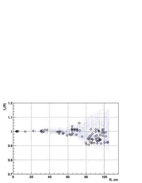
Figure 4: The dependence of the detector light collection function $f_{s}$ on the source distance from the detector’s center. The values of the $f_{s}$ function calculated for the real source positions are shown by stars. Every dot corresponds to the value calculated at center of each 10x10x10 $cm^{3}$ bin using experimental data.

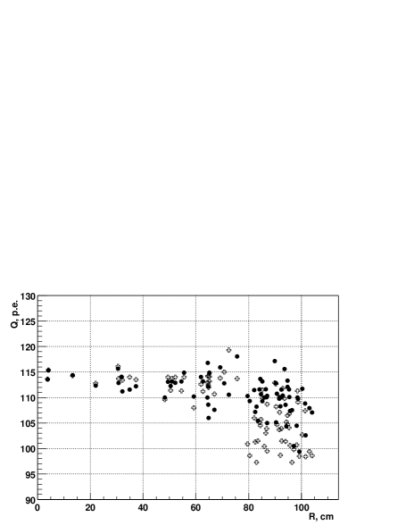
Figure 5: The total charge registered for the different source positions in CTF (crosses). The values of the total charge for the same source positions corrected with the $f_{s}$ function are marked with circles.

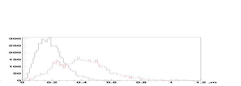
Figure 6: The difference between the nominal source position and the reconstructed one using the charge signals, at different positions inside the detector’s volume: a)$r(0,0,-40)=40$ cm, b)$r(0,0,-80)=80$ cm and c)$r(32,0,105)\simeq 105$ cm (dotted line). For comparison in the same plot the results of reconstruction using time signals only are shown with a solid line. One can see that reconstruction on the charge signals works better than the reconstruction using time signals at large r values.

a)

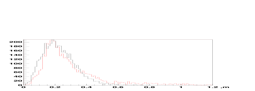
b)

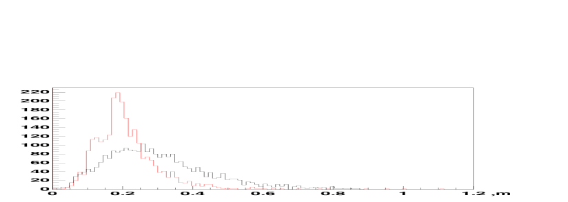
c)

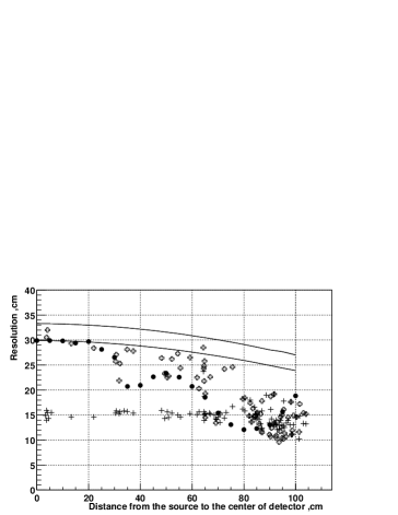
Figure 7: The spatial reconstruction precision (1$\sigma$) using the time data (crosses) and the charge data (empty crosses) as a function of the source distance from the detector’s center (50 PMTs, CTF detector). The results of the calculation using the light collection function estimated from the CTF data are plotted with circles. The two lines corresponds to the calculation using the simplified light collection function (upper solid line) and the simple light collection function with light absorption (lower solid line).

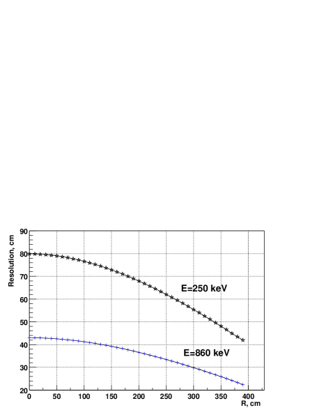
Figure 8: The precision of the spatial reconstruction using charge signals for Borexino as a function of the distance from the source to the detector’s center. The simple light collection function with absorption length of 12 meters has been used in estimations.

Figure 9: The precision of the spatial reconstruction for CTF as a function of $T_{cut}$ for the source energy 250 keV. The time data only are used in estimations. Two sources with different energies have been considered at different source distances from the detector’s center.

Figure 10: The precision of the spatial reconstruction for Borexino as a function of $T_{cut}$ for the source energy 250 keV. The time data only are used in estimations. Two sources with different energies have been considered at different source distances from the detector’s center.

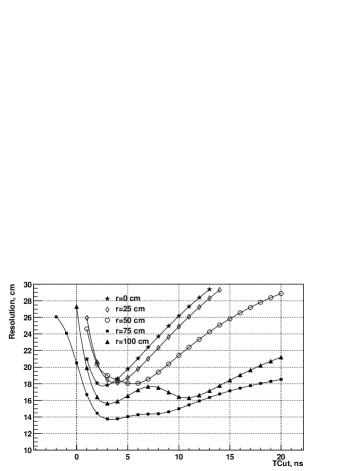
Figure 11: The precision of the spatial reconstruction precision for CTF as a function of $T_{cut}\,$for the source energy 250 keV.The time and charge data are used in estimations. Two sources with different energies have been considered at different source distances from the detector’s center.

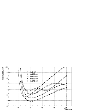
Figure 12: The precision of the spatial reconstruction for Borexino using charge and time data as a function of $T_{cut}\,$for the source energy 250 keV. The time and charge data are used in estimations. Two sources with different energies has been considered at different source distances from the detector’s center.

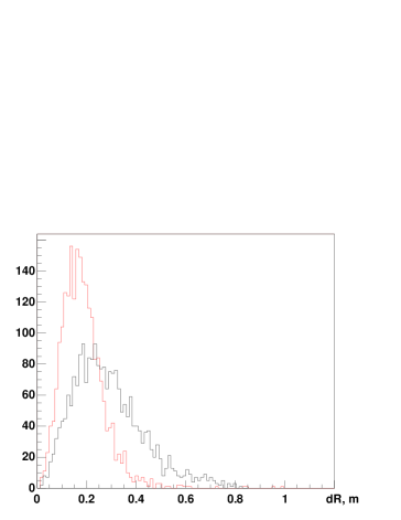
Figure 13: The result of reconstruction of the source position in CTF relative to the nominal source position ($dR$ is the distance between the reconstructed source position and the nominal one) using the time and charge data (dotted line). The artificial radon source is at the position r(4,-63,76)=98 cm from the detector’s center. The distance dR from the reconstructed source position to the nominal one is presented. The plot shows also the reconstruction using the time data only (solid line).

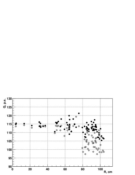
Figure 14: The result of the combined reconstruction (using time and charge data) are shown with circles. The total charge registered for the different source positions, defined as a sum over all PMTs, is shown for comparison (marked by crosses). The reconstruction results are renormalized in order to make the comparison more evident (the point at $r\sim 0$ cm has been used for renormalization). One can see that reconstruction program provides a better base value for the energy evaluation.

References

- [1] Birks J.B., The Theory and Practice of Scintillation Counting (Macmillan, New York, 1964).
- [2] Borexino at Gran Sasso - Proposal for a real time detector for low energy solar neutrino. Volume 1. Edited by G.Bellini, M.Campanella, D.Guigni. Dept. of Physics of the University of Milano. August 1991.
- [3] Lienard E. et al., Nucl. Instrum. and Methods. A413 (1998)321-332.
- [4] Alimonti G. et al., Nucl. Instrum. and Methods. A 406 (1998) p.411-426.
- [5] Suzuki A., Nucl.Phys. B 77(Proc.Suppl.)(1999)171-176.
- [6] G. Ranucci et al., Nucl. Instrum. and Methods. A350 (1994) 338
- [7] Gatti F., Morelli G.,Testera G., Vitale S., Nucl. Instrum. and Methods. A370(1996),p.609
- [8] Johnson M., Benziger J., Stoia C., Calaprice F., Chen M., Darnton N., Loeser F., Vogelaar R.B. Nucl. Instrum. and Methods. A414 (1998) 459.
- [9] Alimonti G., et al. Nucl. Instrum. and Methods. A440 (1998) 360.
- [10] Dossi R., Ianni A., Ranucci G., Smirnov O.Ju., Nucl. Instrum. and Methods. A451 (2000) 623-637.