On Construction of A New Interpolation Tool: Cubic $q$-Spline

Abstract.

This work presents a new interpolation tool, namely, cubic $q$-spline. Our new analogue generalizes a well known classical cubic spline. This analogue, based on the Jackson $q$-derivative, replaces an interpolating piecewise cubic polynomial function by $q$-polynomials of degree three at most. The parameter $q$ provides a solution flexibility.

1. INTRODUCTION

The interpolation problem of an unknown function $f(x)$ when only the values of $f(x_{i})$ at some point $x_{i}$ are given arises in different areas. One of widely used methods is a spline interpolation, and, particularly, cubic spline interpolation. That means that the function $f(x)$ is interpolated between two adjacent points $x_{i}$ and $x_{i+1}$ by a polynomial of degree three at most. Such interpolation is very suitable for smooth functions which do not have oscillating behaviour (cf. [1]). Another advantage of the cubic polynomial interpolation is that it leads to a system of linear equations which is described by a tridiagonal matrix. This linear system has a unique solution which can be fast obtained. A generalization of cubic spline interpolation was done by Marsden (see [2]). He chose a $q$-representation for knots and normalized $B$-splines as interpolating functions. $B$-splines are the generalization of the Bezier curves which are built with the help of Bernstein polynomials and they play an important role in the theory of polynomial interpolation. Their $q$-analogues were defined and studied in [3, 4]. For further information and other details related to q-analogues of Bernstein polynomials, Bezier curves and splines, see the recent works [5, 6, 7, 8, 9, 10]. Another $q$-generalization of polynomial interpolation was studied in [11]. Despite the popularity of $B$-spline, new generalizations of spline continue to appear. Some of them concerns about preserving of convexity [12], some of them about smoothness of interpolation [13], and others about degrees of freedom [14]. Classical cubic spline already proved itself in data and curve fitting problems. Our new $q$-generalization gives it a new interesting twist. The matrix describing the linear system is tridiagonal like in the classic case, and a solution of this linear system can be obtained by simple recursive algorithm (see for example [15]). The $q$-parameter provides a flexibility of the solution.

We start from a short review of definitions coming from the quantum calculus (cf. [16]). The $q$-derivative is given by

$$D_{q}f(x)=\frac{f(qx)-f(x)}{qx-x}.$$

For any complex number $c$, its $q$-analogue is defined as $[c]_{q}=\frac{q^{c}-1}{q-1}$. For natural $n$, a $q$-factorial is defined as $[n]_{q}!=\prod_{k=1}^{n}[k]_{q}$, with $[0]_{q}!=1$.

The $q$-analogue of the polynomial is $(x-c)^{n}_{q}=\prod_{k=1}^{n}(x-cq^{k-1})$ by assuming as usually that $(x-c)^{0}_{q}=1$. It is easy to show that $D_{q}(x-c)^{n}_{q}=[n]_{q}(x-c)^{n-1}_{q}.$ We will denote by $D^{k}_{q}$ the $k$-th $q$-derivative. The Jackson $q$-integral of $f(x)$ is defined as (cf. [16, 17])

$$\int f(x)d_{q}x=(1-q)x\sum_{j=0}^{\infty}q^{j}f(q^{j}x),$$

and $D_{q}\int f(x)d_{q}x=f(x)$. Note that $q$ is usually considered to be $0<q<1$.

In the next section we describe a process of building of a cubic $q$-spline.

2. BUILDING OF A $q$-ANALOGUE OF CUBIC SPLINE

Let a function $f(x)$ is given by its values $f(x_{i})=f_{i}$, $0\leq i\leq n$, at $n+1$ nodes $a=x_{0}<x_{1}<\ldots<x_{n}=b$. We define the cubic $q$-spline function $S\!(x;q)$ as a function of a variable $x$ with parameter $q$ as following:

(1) $$S\!(x;q)=\left\{\begin{array}[]{rl}S_{\!1}(x;q)&x_{0}\leq x\leq x_{1},\\ S_{\!2}(x;q)&x_{1}<x\leq x_{2},\\ \ldots&\ldots\\ S_{\!n}(x;q)&x_{n-1}<x\leq x_{n},\end{array}\right.$$

where each $S_{\!i}(x;q)$, $1\leq i\leq n$, is a $q$-polynomial in variable $x$ of degree at most three, and $S\!(x;q)$, $D_{q}S\!(x;q)$, $D_{q}^{2}S\!(x;q)$ are continuous on $[a,b]$. To provide these properties we demand

(2) $$\left\{\begin{array}[]{ll}S_{\!i}(x_{i-1};q)=f(x_{i-1}),&i=1,\ldots,n,\\ S_{\!i}(x_{i};q)=f(x_{i}),&i=1,\ldots,n,\end{array}\right.$$

(3) $$D_{q}S_{\!i}(x_{i};q)=D_{q}S_{\!{i+1}}(x_{i};q), i=1,\ldots,n-1,$$

(4) $$D_{q}^{2}S_{\!i}(x_{i};q)=D_{q}^{2}S_{\!{i+1}}(x_{i};q), i=1,\ldots,n-1.$$

The boundary conditions for the clamped cubic $q$-spline are

(5) $$\left\{\begin{array}[]{ll}D_{q}S_{\!1}(x_{0};q)=D_{q}f(x_{0}),\\ D_{q}S_{\!n}(x_{n};q)=D_{q}f(x_{n}).\end{array}\right.$$

Let us denote by $\mu_{i}(q)$, $i=0,\ldots,n$ the value of the second $q$-derivative of the spline $S\!(x;q)$ at the node $x_{i}$, that is $\mu_{i}(q)=D_{q}^{2}S\!(x_{i};q)$. Since the spline $S\!(x;q)$ is a polynomial of degree at most three, its second derivative is a polynomial of degree at most one. Therefore it can be written as

$$D_{q}^{2}S_{\!i}(x;q)=\mu_{i-1}(q)\frac{x_{i}-x}{h_{i}}+\mu_{i}(q)\frac{x-x_{i-1}}{h_{i}},$$

where $h_{i}=x_{i}-x_{i-1}$ and $x_{i-1}\leq x\leq x_{i}$ for $1\leq i\leq n$. By performing $q$-integration we obtain

(6) $$D_{q}S_{\!i}(x;q)=\int D_{q}^{2}S_{\!i}(x;q)d_{q}x=\frac{\mu_{i}(q)}{[2]_{q}h_{i}}(x-x_{i-1})^{2}_{q}-\frac{\mu_{i-1}(q)}{[2]_{q}h_{i}}(x-x_{i})^{2}_{q}+A_{i}(q).$$

Let us denote by $f[x_{i-1},x_{i}]=\frac{f(x_{i})-f(x_{i-1})}{x_{i}-x_{i-1}}$ the first order divided difference of a function $f(x)$ at nodes $x_{i-1},x_{i}$. By integrating (6), we obtain

(7) $$S_{\!i}(x;q)=\int D_{q}S_{\!i}(x;q)d_{q}x=\frac{\mu_{i}(q)}{[3]_{q}!h_{i}}(x-x_{i-1})^{3}_{q}-\frac{\mu_{i-1}(q)}{[3]_{q}!h_{i}}(x-x_{i})^{3}_{q}+A_{i}(q)(x-x_{i-1})+B_{i}(q),$$

where $A_{i}(q)$ and $B_{i}(q)$ depend on parameter $q$ only and can be found by substituting $x=x_{i}$ and $x=x_{i-1}$ in (7) respectively and using the conditions (2) as following

(8) $$B_{i}(q) = f(x_{i-1})+\frac{\mu_{i-1}(q)}{[3]_{q}!h_{i}}(x_{i-1}-x_{i})^{3}_{q},$$

(9) $$A_{i}(q) = \frac{f(x_{i})-f(x_{i-1})}{h_{i}}-\frac{\mu_{i}(q)}{[3]_{q}!h_{i}^{2}}(x_{i}-x_{i-1})^{3}_{q}-\frac{\mu_{i-1}(q)}{[3]_{q}!h_{i}^{2}}(x_{i-1}-x_{i})^{3}_{q}.$$

By substituting the detailed expressions (8–9) for functions $A_{i}(q)$ and $B_{i}(q)$, we obtain the $i$th spline function as following

$$S_{\!i}(x;q) = \frac{\mu_{i}(q)}{[3]_{q}!h_{i}}(x-x_{i-1})^{3}_{q}-\frac{\mu_{i-1}(q)}{[3]_{q}!h_{i}}(x-x_{i})^{3}_{q}$$

$$+ \left(f[x_{i-1},x_{i}]-\frac{\mu_{i}(q)}{[3]_{q}!h_{i}^{2}}(x_{i}-x_{i-1})^{3}_{q}-\frac{\mu_{i-1}(q)}{[3]_{q}!h^{2}_{i}}(x_{i-1}-x_{i})^{3}_{q}\right)(x-x_{i-1})$$

$$+ f(x_{i-1})+\frac{\mu_{i-1}(q)}{[3]_{q}!h_{i}}(x_{i-1}-x_{i})^{3}_{q}.$$

In order to obtain the unknown moments $\mu_{i}(q)$, $i=0,\ldots,n$ we use the conditions (3) for the first derivative of the $q$-spline (6). Hence, for $i=1,\dots,n-1$, we have

(11) $$\frac{\mu_{i}(q)}{[2]_{q}h_{i}}(x_{i}-x_{i-1})^{2}_{q} + f[x_{i-1},x_{i}]-\frac{\mu_{i}(q)}{[3]_{q}!h_{i}^{2}}(x_{i}-x_{i-1})^{3}_{q}-\frac{\mu_{i-1}(q)}{[3]_{q}!h_{i}^{2}}(x_{i-1}-x_{i})^{3}_{q}$$

$$= -\frac{\mu_{i}(q)}{[2]_{q}h_{i+1}}(x_{i}-x_{i+1})^{2}_{q}+f[x_{i},x_{i+1}]-\frac{\mu_{i+1}(q)}{[3]_{q}!h_{i+1}^{2}}(x_{i+1}-x_{i})^{3}_{q}$$

$$- \frac{\mu_{i}(q)}{[3]_{q}!h_{i+1}^{2}}(x_{i}-x_{i+1})^{3}_{q}.$$

Moreover, from the boundary conditions (5) for the clamped $q$-spline we obtain

(12) $$D_{q}S_{\!1}(x_{0};q) = -\frac{\mu_{0}(q)}{[2]_{q}h_{1}}(x_{0}-x_{1})^{2}_{q}+f[x_{0},x_{1}]$$

$$- \frac{\mu_{1}(q)}{[3]_{q}!h_{1}^{2}}(x_{1}-x_{0})^{3}_{q}-\frac{\mu_{0}(q)}{[3]_{q}!h_{1}^{2}}(x_{0}-x_{1})^{3}_{q}=D_{q}f(x_{0}),$$

(13) $$D_{q}S_{\!n}(x_{n};q) = \frac{\mu_{n}(q)}{[2]_{q}h_{n}}(x_{n}-x_{n-1})^{2}_{q}+f[x_{n-1},x_{n}]$$

$$- \frac{\mu_{n}(q)}{[3]_{q}!h^{2}_{n}}(x_{n}-x_{n-1})^{3}_{q}-\frac{\mu_{n-1}(q)}{[3]_{q}!h_{n}^{2}}(x_{n-1}-x_{n})^{3}_{q}=D_{q}f(x_{n}).$$

The equations (11–13) form a system of $(n+1)$ linear equations with respect to the moments $\mu_{i}(q)$ that can be written shortly as $A\mu=b$. With the notation $\mathcal{H}_{i}(q)=\frac{(qx_{i}-x_{i-1})(x_{i}-qx_{i-1})}{x_{i}-x_{i-1}}$, we have

(14) $$A=\left(\begin{array}[]{cccccc}[2]_{q}\mathcal{H}_{1}(q)&\frac{(x_{1}-qx_{0})^{2}_{q}}{x_{1}-x_{0}}&0&0&\ldots&0\\ \frac{(x_{0}-qx_{1})^{2}}{x_{1}-x_{0}}&[2]_{q}(\mathcal{H}_{1}(q)+\mathcal{H}_{2}(q))&\frac{(x_{2}-qx_{1})^{2}_{q}}{x_{2}-x_{1}}&0&\ldots&0\\ \ldots&\ldots&\ldots&\ldots&\ldots&\ldots\\ 0&0&0&0&\frac{(x_{n-1}-qx_{n})^{2}_{q}}{x_{n}-x_{n-1}}&[2]_{q}\mathcal{H}_{n}(q)\end{array}\right),$$

(15) $$b=[3]_{q}!\left(\begin{array}[]{c}f[x_{0},x_{1}]-D_{q}f(x_{0})\\ f[x_{1},x_{2}]-f[x_{0},x_{1}]\\ \vdots\\ f[x_{n-1},x_{n}]-f[x_{n-2},x_{n-1}]\\ D_{q}f(x_{n})-f[x_{n-1},x_{n}]\end{array}\right),\quad\quad\mu=\left(\begin{array}[]{c}\mu_{0}(q)\\ \vdots\\ \mu_{n}(q)\end{array}\right).$$

The unknown moments $\mu=\mu(q)$ (15) are the solution of the matrix equation $A\mu=b$, where $A$ is given by (14) and $b$ is given by (15). In view of the fact that $A$ is a tridiagonal matrix, the method proposed in [15] may be used for evaluating the moments $\mu_{i}(q)$, $i=0..,n$.

The moments $\mu_{i}(q)$, $i=0,\ldots,n$ are the solution of the matrix equation $A\mu=b$, therefore they are the unique functions of parameter $q$. Thus we can state the following result.

Theorem 1.

Let the piecewise function $S\!(x;q)$ be defined by (1) and (2), where $\mu=\mu(q)$ is a unique solution of the matrix equation $A\mu=b$, with $A$ given by (14) and $b$ given by (15). Then $S\!(x;q)$ is a $q$-analogue of the cubic spline interpolation of a function $f(x)$.

Example 2.

Let us consider a $q$-spline interpolation of a function $f(x)=x^{4}$ on the interval $x\in[-1,1]$ at the knots $x_{0}=-1$, $x_{1}=0$, $x_{2}=1$. We assume that the values of the function itself and its first derivation at the knots are given. The classical cubic spline solution is given in Example 1 on page 824–825 of [18]. By using the above proposed method, one can obtain the cubic $q$-spline solution:

$$S(x;q)=\left\{\begin{array}[]{lcl}\frac{q^{3}-3q^{2}-2q-2}{2q^{2}+q}x^{3}+\frac{q^{3}-q^{2}-q-2}{2q^{2}+q}x^{2},&&-1\leq x\leq 0,\\ -\frac{q^{3}-3q^{2}-2q-2}{2q^{2}+q}x^{3}+\frac{q^{3}-q^{2}-q-2}{2q^{2}+q}x^{2},&&0\leq x\leq 1.\end{array}\right.$$

It is easy to obtain the classical cubic spline solution corresponding to $q\rightarrow 1$. One can see that there exist a slight oscillation of the spline regarding to the original function. Decreasing the parameter $q$ leads to more intensive oscillation. However, increasing the parameter $q$ overcomes the oscillation effect and interpolates the original function with significant improvement.

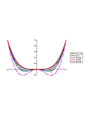
Figure 1. Interpolation of $f(x)=x^{4}$ by cubic $q$-spline.

3. ACKNOWLEDGMENTS

This research was supported by the Ministry of Science and Technology, Israel.

The author thanks to the anonymous referees for their advices.

References

[1]
K. Atkinson, An introduction to numerical analysis,
Wiley, 2nd ed., 1989.
[2]
M.J. Marsden, Spline interpolation at knot averages on a two-sided geometric mesh,
Math. Comput.,
38 (157), 113–126 (1982).
[3]
G. Budakçi, Ç. Disibüyük, R. Goldman, and H. Oruç,
Extending fundamental formulas from classical B-splines to quantum B-splines,
J. Comput. Appl. Math., 282, 17–33 (2015).
[4]
P. Simeonov and R. Goldman, Quantum B-splines,
BIT Numer. Math., 53 (1), 193–223 (2013).
[5]
R. Goldman, P. Simeonov, and Y. Simsek, Generating functions for the -Bernstein bases, SIAM J. Discrete Math.28 (3), 1009–1025 (2014).
[6]
R. Goldman and P. Simeonov, Quantum Bernstein bases and quantum Bezier curves, J. Comput. Appl. Math.288, 284–303 (2015).
[7]
R. Goldman and P. Simeonov, Generalized quantum splines, Comp. Aided Geom. Design47, 29–54 (2016).
[8]
H. Oruç and G.M. Phillips, -Bernstein polynomials and Bezier curves, J. Comput. Appl. Math.151 (1), 1–12 (2003).
[9]
S. Ostrovska, -Bernstein polynomials and their iterates, J. Approx. Theory123 (2), 232–255 (2003).
[10]
P. Simeonov, V. Zafiris, and R. Goldman, -blossoming: a new approach to algorithms and identities for -Bernstein bases and -Bezier curves, J. Approx. Theory164 (1), 77–104 (2012).
[11]
Y. Simsek, Interpolation function of generalized -Bernstein-type basis polynomials and applications, in: Proceedings of the 7th International Conference on Curves and Surfaces, 647–662 (2012).
[12]
X. Han, Convexity-preserving approximation by univariate cubic splines, J. Comput. Appl. Math.,
287, 196–206 (2015).
[13]
K. Segeth, Some splines produced by smooth interpolation, Appl. Math. Comput.,
319, 387–394 (2018).
[14]
P.O. Mohammed and F.K. Hamasalh, Twelfth degree spline with application to quadrature,
SpringerPlus, 5:2096 (2016).
[15]
E. Kiliç, Explicit formula for the inverse of a tridiagonal matrix by backward continued fractions, Appl. Math. Comput., 197 (1), 345–357 (2008).
[16]
V. Kac and P. Cheung,
Quantum calculus, Springer-Verlag, 2002.
[17]
F.H. Jackson, On -definite integrals, Q. J. Pure Appl. Math.41, 193–203 (1910).
[18]
E. Kreyszig,
Advanced engineering mathematics, Willey, 10th ed., 2011.