Low-lying collective excited states in non-integrable pairing models based on stationary-phase approximation to path integral

Abstract

For a description of large-amplitude collective motion associated with nuclear pairing, requantization of time-dependent mean-field dynamics is performed using the stationary-phase approximation (SPA) to the path integral. We overcome the difficulty of the SPA, which is known to be applicable to integrable systems only, by developing a requantization approach combining the SPA with the adiabatic self-consistent collective coordinate method (ASCC+SPA). We apply the ASCC+SPA to multi-level pairing models, which are non-integrable systems, to study the nuclear pairing dynamics. The ASCC+SPA gives a reasonable description of low-lying excited $0^{+}$ states in non-integrable pairing systems.

I Introduction

Pairing correlation plays an important role in open-shell nuclei. Effect of the pairing is prominent in many observables for the ground states, such as the odd-even mass difference, moment of inertia of rotational bands, and common quantum number $J^{\pi}=0^{+}$ for even-even nuclei Ring and Schuck (1980). Collective excitations associated with the pairing, such as pair vibrations and pair rotations, have been observed in a number of nuclei Brink and Broglia (2005). Most of these states that are “excited” from neighboring even-even systems are associated with the ground $J^{\pi}=0^{+}$ states in even-even nuclei. In contrast, properties of excited $J^{\pi}=0^{+}$ states are not clearly understood yet Heyde and Wood (2011); Garrett (2001), for which the pairing dynamics plays an important role in a low-energy region (a few MeV excitation) of nuclei. In this paper, we aim to understand the dynamics associated with pairing correlation in nuclei from a microscopic view point.

The time-dependent mean-field (TDMF) theory is a standard theory to describe the dynamics of nuclei from the microscopic degrees of freedom. Inclusion of the pairing dynamics leads to the time-dependent Hartree-Fock-Bogoliubov (TDHFB) theory, which has been utilized for a number of studies of nuclear reaction and structure Nakatsukasa et al. (2016). The small-amplitude approximation of the TDHFB with modern energy density functionals, the quasiparticle random-phase approximation (QRPA), has successfully reproduced the properties of giant resonances in nuclei. In contrast, the QRPA description of low-lying quadrupole vibrations is not as good as that of giant resonances Nakatsukasa et al. (2016). A large-amplitude nature of the quantum shape fluctuation is supposed to be important for these low-lying collective states. Five-dimensional collective Hamiltonian (5DCH) approaches have been developed for studies of low-lying quadrupole states, in which the collective Hamiltonian is constructed from microscopic degrees of freedom using the mean-field calculation and the cranking formula for the inertial masses Baran et al. (2011); Delaroche et al. (2010); Fu et al. (2013). The 5DCH model is able to take into account fluctuations of the quadrupole shape degrees of freedom which are important in many nuclear low-energy phenomena, such as shape coexistence and anharmonic quadrupole vibration. However, the calculated inertia is often too small to reproduce experimental data, due to the lack of time-odd components in the cranking formula Ring and Schuck (1980). This deficiency can be remedied in the adiabatic self-consistent collective coordinate (ASCC) method Matsuo et al. (2000), in which the time-odd effect is properly treated. In addition, the ASCC method enables us to identify a collective subspace of interest. The ASCC was developed from the basic idea of the self-consistent collective coordinate (SCC) method by Marumori and coworkers Marumori et al. (1980). It has been applied to the nuclear quadrupole dynamics including the shape coexistence Kobayasi et al. (2005); Hinohara et al. (2008, 2009).

The TDMF (TDHFB) theory corresponds to an SPA solution in the path integral formulation Negele (1982). It lacks a part of quantum fluctuation that is important in the large-amplitude dynamics. To introduce the quantum fluctuation based on the TDHFB theory, the requantization is necessary Negele (1982); Levit (1980); Levit et al. (1980); Reinhardt (1980); Kuratsuji and Suzuki (1980); Kuratsuji (1981). A simple and straightforward way of requantization is the canonical quantization. This is extensively utilized for collective models in nuclear physics. For instance, the canonical quantization of the 5DCH was employed for the study of low-lying excited states in nuclei Próchniak and Rohoziński (2009); Hinohara et al. (2010); Nakatsukasa et al. (2016). The similar quantization was also utilized for the pairing collective Hamiltonian Bès et al. (1970); Góźdź et al. (1985); Zaja̧c et al. (1999); Pomorski (2007). In our previous work Ni and Nakatsukasa (2018), we studied various requantization methods for the two-level pairing model, to investigate low-lying excited $0^{+}$ states. Since the collectivity is rather low in the pairing motion in nuclei, the canonical quantization often fails to produce an approximate value to the exact solution. In contrast, the stationary-phase approximation (SPA) to the path integral Suzuki and Mizobuchi (1988) can give quantitative results not only for the excitation energies, but also for the wave functions and two-particle-transfer strengths. The quantized states obtained in the SPA have two advantages; first, the wave functions are given directly in terms of the microscopic degrees of freedom, and second, the restoration of the broken symmetries are automatic. In the pairing model, the quantized states are eigenstates of the particle-number operator. On the other hand, applications of the SPA have been limited to integrable systems. This is because we need to find separable periodic trajectories on a classical torus. Since the nuclear systems, of course, correspond to non-integrable systems, a straightforward application of the SPA is not possible.

In this paper, we propose a new approach of the SPA applicable to the non-integrable systems, which is based on the extraction of the one-dimensional (1D) collective coordinate using the ASCC method. Since the 1D system is integrable, the collective subspace can be quantized with the SPA. The optimal degree of freedom associated with a slow collective motion is determined self-consistently inside the TDHFB space, without any assumption. Thus, our approach of the ASCC+SPA to the pairing model basically consists of two steps: (1) find a decoupled 1D collective coordinate of the pair vibration, in addition to the pair rotational degrees of freedom. (2) apply the SPA independently to each collective mode.

The paper is organized as follows. Section II introduces the theoretical framework of the ASCC, SPA, and their combination, ASCC+SPA. In Sec. III, we provide some details in the application of the ASCC+SPA to the multi-level pairing model. We give the numerical results in Sec. IV, including neutron pair vibrations in Pb isotopes. The conclusion and future perspectives are given in Sec. V.

II Theoretical framework

II.1 Adiabatic self-consistent collective coordinate method and 1D collective subspace

In this section, we first recapitulate the ASCC method to find a 1D collective coordinate, following the notation of Ref. Nakatsukasa (2012).

As is seen in Sec. III, the TDHFB equations can be interpreted as the classical Hamilton’s equations of motion with canonical variables $\{\xi^{\alpha},\pi_{\alpha}\}$. Each point in the phase space $(\xi^{\alpha},\pi_{\alpha})$ corresponds to a generalized Slater determinant (coherent state). Assuming slow collective motion, we expand the Hamiltonian $\mathcal{H}(\xi,\pi)$ with respect to the momenta $\pi$ up to second order. The TDHFB Hamiltonian is written as

$$\mathcal{H} =V(\xi)+\frac{1}{2}B^{\alpha\beta}(\xi)\pi_{\alpha}\pi_{\beta}$$ (2.1)

with the potential $V(\xi)$ and the reciprocal mass parameter $B^{\alpha\beta}(\xi)$ defined by

$$V(\xi) =\mathcal{H}(\xi,\pi=0),$$ (2.2)

$$B^{\alpha\beta}(\xi) =\left.\frac{\partial^{2}\mathcal{H}(\xi,\pi)}{\partial\pi_{\alpha}\partial\pi_{\beta}}\right|_{\pi=0}.$$ (2.3)

For multi-level pairing models in Sec. III, there is a constant of motion in the TDHFB dynamics, namely the average particle number $q^{n}\equiv\langle\hat{N}\rangle/2$. Since the particle number $\hat{N}$ is time-even Hermitian operator, we treat this as a coordinate, and its conjugate gauge angle, $p_{n}$, as a momentum. Since $q^{n}$ is a constant of motion, the Hamiltonian does not depend on $p_{n}$. On the other hand, the gauge angle $p_{n}$ changes in time, which corresponds to the pair rotation, a Nambu-Goldstone (NG) mode associated with the breaking of the gauge (particle-number) symmetry. We assume the existence of 2D collective subspace $\Sigma_{2}$ (4D phase space), described by a set of canonical variable $(q^{1},q^{2}=q^{n};p_{1},p_{2}=p_{n})$, which is well decoupled from the rest of degrees of freedom, $\{q^{a},p_{a}\}$ with $a=3,\cdots$. The collective Hamiltonian is given by imposing $q^{a}=p_{a}=0$, namely by restricting the space into the collective subspace

$$\mathcal{H}_{\rm coll}(q,p;q^{n})=\bar{V}(q^{1},q^{n})+\frac{1}{2}\bar{B}^{11}(q^{1},q^{n})p_{1}^{2}.$$ (2.4)

Since there exist two conserved quantities, $q^{n}$ and $\mathcal{H}_{\rm coll}$, this 2D system is integrable. We can treat the collective motion of $(q^{1},p_{1})$ separately from the pair rotation $(q^{n},p_{n})$.

In the collective Hamiltonian (2.4), the variable $q^{n}$ is trivially given as the particle number, which is expanded up to second order in the momenta $\pi$,

$$q^{n}=\frac{\langle\hat{N}\rangle}{2}=f^{n}(\xi)+\frac{1}{2}f^{(1)n\alpha\beta}\pi_{\alpha}\pi_{\beta}.$$ (2.5)

To obtain the non-trivial collective variables $(q^{1},p_{1})$, we assume the point transformation,

$$q^{1}=f^{1}(\xi),$$ (2.6)

and $\xi^{\alpha}$ on the subspace $\Sigma_{2}$ is given as $\xi^{\alpha}=g^{\alpha}(q^{1},q^{n},q^{a}=0)$. The momenta on $\Sigma_{2}$ are transformed as

$$p_{1} =g_{,1}^{\alpha}\pi_{\alpha},\quad p_{n}=g_{,n}^{\alpha}\pi_{\alpha},$$ (2.7)

$$\pi_{\alpha} =f^{1}_{,\alpha}p_{1}+f^{n}_{,\alpha}p_{n},$$ (2.8)

where the comma indicates the partial derivative $(f^{1}_{,\alpha}=\partial f^{1}/\partial\xi^{\alpha})$. The Einstein’s convention for summation with respect to the repeated upper and lower indices is assumed hereafter. The canonical variable condition leads to

$$f^{i}_{,\alpha}g_{,j}^{\alpha}=\delta^{i}_{j},$$ (2.9)

where $i,j=1$ and $n$. The collective potential $\bar{V}(q^{1},q^{n})$ and the collective mass parameter $\bar{B}_{11}(q^{1},q^{n})=[\bar{B}^{11}(q^{1},q^{n})]^{-1}$ can be given by

$$\bar{V}(q^{1},q^{n}) =V(\xi=g(q^{1},q^{n},q^{a}=0)),$$ (2.10)

$$\bar{B}^{11}(q^{1},q^{n}) =f^{1}_{,\alpha}\tilde{B}^{\alpha\beta}(\xi)f^{1}_{,\beta},$$ (2.11)

where $\tilde{B}^{\alpha\beta}$ are defined as

$$\tilde{B}^{\alpha\beta}(\xi) =B^{\alpha\beta}(\xi)-\bar{V}_{,n}f^{(1)n\alpha\beta}(\xi).$$ (2.12)

Decoupling conditions for the collective subspace $\Sigma_{2}$ lead to the basic equations of the ASCC method Matsuo et al. (2000); Nakatsukasa (2012), which determine tangential vectors, $f^{1}_{,\alpha}(\xi)$ and $g_{,1}^{\alpha}(q)$.

$$\delta H_{M}(\xi,\pi)=0,$$ (2.13)

$$\mathcal{M}^{\beta}_{\alpha}f^{1}_{,\beta}=\omega^{2}f^{1}_{,\alpha},\hskip 20.00003pt\mathcal{M}^{\beta}_{\alpha}g^{\alpha}_{,1}=\omega^{2}g^{\beta}_{,1}.$$ (2.14)

The first equation (2.13) is called moving-frame Hartree-Fock-Bogoliubov (HFB) equation. The moving-frame Hamiltonian $\mathcal{H}_{M}$ is

$$\mathcal{H}_{M}(\xi,\pi) =\mathcal{H}(\xi,\pi)-\lambda_{1}q^{1}(\xi)-\lambda_{n}q^{n}(\xi,\pi).$$ (2.15)

The second equation (2.14) is called moving-frame QRPA equation. The matrix $\mathcal{M}^{\beta}_{\alpha}$ in the moving-frame QRPA equation (2.14) can be rewritten as

$$\mathcal{M}^{\beta}_{\alpha}=\tilde{B}^{\beta\gamma}\left(V_{,\gamma\alpha}-\lambda_{n}f^{n}_{,\gamma\alpha}\right)+\frac{1}{2}\tilde{B}^{\beta\gamma}_{,\alpha}V_{,\gamma}.$$ (2.16)

The NG mode, $f^{n}_{,\alpha}$ and $g^{\alpha}_{,n}$, corresponds to the zero mode with $\omega^{2}=0$. Therefore, the collective mode of our interest corresponds to the mode with the lowest frequency squared except for the zero mode.

In practice, we obtain the collective path according to the following procedure:

1. Find the HFB minimum point $\xi^{\alpha}_{i}$ ($i=0$) by solving Eq. (2.13) with $\lambda_{1}=0$. Let us assume that this corresponds to $q^{1}_{i}=0$.

2. Diagonalize the matrix $\mathcal{M}^{\beta}_{\alpha}$ to solve Eq. (2.14) using Eq. (2.16).

3. Move to the next neighboring point $\xi^{\alpha}_{i+1}=\xi^{\alpha}_{i}+d\xi^{\alpha}$ with $d\xi^{\alpha}=g^{\alpha}_{,1}dq^{1}$. This corresponds to the collective coordinate, $q^{1}_{i+1}=q^{1}_{i}+dq^{1}$.

4. At $\xi_{i+1}^{\alpha}$ $(q^{1}_{i+1})$, obtain a self-consistent solution of Eqs. (2.13) and (2.14) to determine $\xi^{\alpha}_{i+1}$, $f^{1}_{,\alpha}$, and $g^{\alpha}_{,1}$.

5. Go back to Step 3 to determine the next point on the collective path.

We repeat this procedure with $dq^{1}>0$ and $dq^{1}<0$, and construct the collective path. In Steps 2 and 4, we choose a mode with the lowest frequency squared $\omega^{2}$. Note that $\omega^{2}$ can be negative. In Step 4, when we solve Eq. (2.13), we use a constraint on the magnitude of $dq^{1}=f^{1}_{,\alpha}d\xi^{\alpha}$. Since the normalization of $f^{1}_{,\alpha}$ and $g^{\alpha}_{,1}$ is arbitrary as far as they satisfy Eq. (2.9), we fix this scale by an additional condition of $\bar{B}^{11}(q^{1})=1$.

II.2 Stationary-phase approximation to path integral

For quantization of integrable systems, we can apply the stationary-phase approximation (SPA) to the path integral. In our former study Ni and Nakatsukasa (2018), we have proposed and tested the SPA for an integrable pairing model. Since the collective Hamiltonian (2.4) that is extracted from the TDHFB degrees of freedom is integrable, the SPA is applicable to it. In this manner, we may apply the ASCC+SPA to non-integrable systems in general.

II.2.1 Basic idea of ASCC+SPA

Because the Hamiltonian $\mathcal{H}_{\rm coll}$ of Eq. (2.4) is separable, it is easy to find periodic trajectories on invariant tori. Since the pair rotation corresponds to the motion of $p_{n}$ with a constant $q^{n}$, all we need to do is to find classical periodic trajectories $C_{k}$ in the $(q^{1},p_{1})$ space (with a fixed $q^{n}$) which satisfy the Einstein-Brillouin-Keller (EBK) quantization rule with a unit of $\hbar=1$,

$$\oint_{C_{k}}p_{1}dq^{1}=2\pi k,$$ (2.17)

where $k$ is an integer number.

At each point in the space $(q^{1},q^{n};p_{1},p_{n})$ corresponds to a generalized Slater determinant $\ket{q^{1},q^{n};p_{1},p_{n}}=\ket{\xi,\pi}$ where $(\xi,\pi)$ are given as $\xi^{\alpha}=g^{\alpha}(q^{1},q^{n},q^{a}=0)$ and $\pi_{\alpha}=f^{1}_{,\alpha}p_{1}+f^{n}_{,\alpha}p_{n}$. According to the SPA, the $k$-th excited state $\ket{\psi_{k}}$ is constructed from the $k$-th periodic trajectory $C_{k}$, given by $(q^{1}(t),p_{1}(t))$, of the Hamiltonian $\mathcal{H}_{\rm coll}$.

$$\ket{\psi_{k}}\propto\oint dp_{n}\oint_{C_{k}}\rho(q,p)dt\ket{q,p}e^{i\mathcal{T}[q,p]},$$ (2.18)

where $(q,p)$ means $(q^{1},q^{n};p_{1},p_{n})$, and the weight function $\rho(q,p)$ is given through an invariant measure $d\mu(q,p)$ as

$$d\mu(q,p)=\rho(q,p)dEdtdq^{n}dp_{n}.$$ (2.19)

The invariant measure $d\mu(q,p)$ is defined by the unity condition $\int d\mu(q,p)\ket{q,p}\bra{q,p}=1$. An explicit form of $d\mu(q,p)$ for the present pairing model is shown in Eq. (3.21). The action integral $\mathcal{T}$ is defined by

$$\mathcal{T}[q,p] \equiv\int_{0}^{t}\braket{q(t^{\prime}),p(t^{\prime})}{i\frac{\partial}{\partial t^{\prime}}}{q(t^{\prime}),p(t^{\prime})}dt^{\prime}.$$ (2.20)

The SPA quantization is able to provide a wave function $\ket{\psi_{k}}$ in microscopic degrees of freedom, which is given as a superposition of generalized Slater determinants $\ket{q,p}$. In addition, the integration with respect to $p_{n}$ over a circuit on a torus automatically recovers the broken symmetry, namely the good particle number. However, it relies on the existence of invariant tori. In the present approach of the ASCC+SPA, we first derive a decoupled collective subspace $\Sigma_{2}$ and identify canonical variables $(q,p)$. Because of the cyclic nature of $(q^{n},p_{n})$, it is basically a 1D system and becomes integrable. In other words, we perform the torus quantization on approximate tori in the TDHFB phase space $(\xi,\pi)$, which is mapped from tori in the 2D collective subspace $(q,p)$.

II.2.2 Notation and practical procedure for quantization

For the application of the ASCC+SPA method to the pairing model in Sec. III, we summarize some notations and procedures to obtain quantized states.

In Sec. III, the time-dependent generalized Slater determinants (coherent states) are written as $\ket{Z}$ with complex variables $Z_{\alpha}(t)$. The variables $Z_{\alpha}$ are transformed into real variables $(j^{\alpha},-\chi_{\alpha})$ that correspond to $(\xi^{\alpha},\pi_{\alpha})$ in Sec. II. $\chi_{\alpha}$ and $j^{\alpha}$ correspond to the “angle” and the “number” variables, respectively. Although it is customary to take the time-odd angle $\chi_{\alpha}$ as a coordinate, we take the number $j^{\alpha}$ as a coordinate and the angle $-\chi_{\alpha}$ as a momentum with an additional minus sign. Similarly, the gauge angle $\Phi$ and the total particle number $J$ correspond to variables of the pair rotation, $-p_{n}$ and $q^{n}$, respectively.

According to the EBK quantization rule (2.17), the ground state with $k=0$ corresponds to nothing but the HFB state with a fixed particle number $J(=q^{n})$. For the $k$-th excited states, we perform the following calculations:

1. Obtain the 1D collective subspace with canonical variables $(q^{1},p_{1})$ according to the ASCC in Sec. II.1.

2. Find a trajectory $(q^{1}(t),p_{1}(t))$ which satisfies the $k$-th EBK quantization condition (2.17).

3. Calculate the action integral (2.20) for the $k$-th trajectory.

4. Construct the $k$-th excited state using Eq. (2.18).

The ASCC provides the 2D collective subspace $(q^{1},J)$ and the generalized coherent states $\ket{\Phi=0,J;q,p=0}$. For finite values of momenta, we use Eq. (2.8) to obtain the state $\ket{\Phi,J;q,p}$.

III Pairing model

We study the low-lying excited $0^{+}$ states in the multi-level pairing model by applying the ASCC+SPA. The Hamiltonian of the pairing model is given in terms of the single-particle energies $\epsilon_{l}$ and the pairing strength $g$ as

$$\hat{H} =\sum_{\alpha}\epsilon_{\alpha}\hat{n}_{\alpha}-g\sum_{\alpha,\beta}\hat{S}_{\alpha}^{+}\hat{S}_{\beta}^{-}$$

$$=\sum_{\alpha}\epsilon_{\alpha}(2\hat{S}_{\alpha}^{0}+\Omega_{\alpha})-g\hat{S}^{+}\hat{S}^{-},$$ (3.1)

where we use the SU(2) quasi-spin operators, $\boldsymbol{\hat{S}}=\sum_{\alpha}\boldsymbol{\hat{S}}_{\alpha}$, with

$$\hat{S}_{\alpha}^{0} = \frac{1}{2}\left(\sum_{m}\hat{a}_{j_{\alpha}m}^{{\dagger}}\hat{a}_{j_{\alpha}m}-\Omega_{\alpha}\right),$$ (3.2)

$$\hat{S}_{\alpha}^{+} = \sum_{m>0}\hat{a}_{j_{\alpha}m}^{{\dagger}}\hat{a}_{j_{\alpha}\overline{m}}^{{\dagger}},\quad\hat{S}_{\alpha}^{-}=\hat{S}_{\alpha}^{+{\dagger}}.$$ (3.3)

Each single-particle energy $\epsilon_{\alpha}$ possesses $2\Omega_{\alpha}$-fold degeneracy ($\Omega_{\alpha}=j_{\alpha}+1/2$) and $\sum_{m>0}$ indicates the summation over $m=1/2,3/2,\cdots,$ and $\Omega_{\alpha}-1/2$. The occupation number of each level $\alpha$ is given by $\hat{n}_{\alpha}=\sum_{m}\hat{a}^{{\dagger}}_{j_{\alpha}m}\hat{a}_{j_{\alpha}m}=2\hat{S}_{\alpha}^{0}+\Omega_{\alpha}$. The quasi-spin operators satisfy the commutation relations

$$[\hat{S}_{\alpha}^{0},\hat{S}_{\beta}^{\pm}]=\pm\delta_{\alpha\beta}\hat{S}_{\alpha}^{\pm},\quad[\hat{S}_{\alpha}^{+},\hat{S}_{\beta}^{-}]=2\delta_{\alpha\beta}\hat{S}_{\alpha}^{0}.$$ (3.4)

The magnitude of quasi-spin for each level is given by $S_{\alpha}=\frac{1}{2}(\Omega_{\alpha}-\nu_{\alpha})$, where $\nu_{\alpha}$ is the seniority quantum number, namely the number of unpaired particles at the level $\alpha$. In the present study, we consider only seniority-zero states with $\nu=\sum_{\alpha}\nu_{\alpha}=0$. The residual two-body interaction consists of the monopole pairing interaction which couples two particles to zero angular momentum. We obtain the exact solutions either by solving the Richardson equation Richardson (1963); Richardson and Sherman (1964a, b) or by diagonalizing the Hamiltonian using the quasi-spin symmetry.

III.1 Classical form of TDHFB Hamiltonian

The time-dependent coherent state for the seniority $\nu=0$ states ($S_{\alpha}=\Omega_{\alpha}/2$) is constructed with time-dependent complex variables $Z_{\alpha}(t)$ as

$$\ket{Z(t)}=\prod_{\alpha}\left(1+|Z_{\alpha}(t)|^{2}\right)^{-\Omega_{\alpha}/2}\exp[Z_{\alpha}(t)\hat{S}_{\alpha}^{+}]\ket{0},$$ (3.5)

where $\ket{0}$ is the vacuum (zero-particle) state. The TDHFB motion is given by the time development of $Z_{\alpha}(t)$. In the SU(2) quasi-spin representation, $\ket{0}=\prod_{\alpha}\ket{S_{\alpha},-S_{\alpha}}$. The coherent state $\ket{Z(t)}$ is a superposition of the states with different particle numbers without unpaired particles. In the present pairing model, the coherent state is the same as the time-dependent BCS wave function with $Z_{\alpha}(t)=v_{\alpha}(t)/u_{\alpha}(t)$, where $(u_{\alpha}(t),v_{\alpha}(t))$ are the time-dependent BCS $u,v$ factors.

The TDHFB equation can be derived from the time-dependent variational principle, $\delta\mathcal{S}=0$, where

$$\mathcal{S}\equiv\int\mathcal{L}(t)dt=\int\braket{Z(t)}{i\frac{\partial}{\partial t}-\hat{H}}{Z(t)}dt$$ (3.6)

($\hbar=1$ applies hereafter). After the transformation of the complex variables into the real ones with $Z_{\alpha}=\tan{\frac{\theta_{\alpha}}{2}}e^{-i\chi_{\alpha}}$ ($0\leq\theta_{\alpha}\leq\pi$), the Lagrangian $\mathcal{L}$ and the expectation value of the Hamiltonian are written as

$$\mathcal{L}(t)=\sum_{\alpha}\frac{\Omega_{\alpha}}{2}(1-\cos{\theta}_{\alpha})\dot{\chi}_{\alpha}-\mathcal{H}(Z,Z^{*}),$$ (3.7)

with

$$\mathcal{H}( Z,Z^{*})\equiv\braket{Z}{\hat{H}}{Z}$$

$$= \sum_{\alpha}\epsilon_{\alpha}\Omega_{\alpha}(1-\cos{\theta}_{\alpha})$$

$$-\frac{g}{4}\sum_{\alpha}\Omega_{\alpha}[\Omega_{\alpha}(1-\cos^{2}{\theta}_{\alpha})+(1-\cos{\theta}_{\alpha})^{2}]$$

$$-\frac{g}{4}\sum_{\alpha\neq\beta}\Omega_{\alpha}\Omega_{\beta}\sqrt{(1-\cos^{2}{\theta}_{\alpha})(1-\cos^{2}{\theta}_{\beta})}e^{-i(\chi_{\alpha}-\chi_{\beta})}.$$ (3.8)

We choose $\chi_{\alpha}$ as canonical coordinates, and their conjugate momenta are given by

$$j^{\alpha}\equiv\frac{\partial\mathcal{L}}{\partial\dot{\chi}_{\alpha}}=\frac{\Omega_{\alpha}}{2}(1-\cos{\theta}_{\alpha}).$$ (3.9)

$\chi_{\alpha}$ represents a kind of gauge angle of each level, and $j^{\alpha}$ corresponds to the occupation number of each level, $2j^{\alpha}=\bra{Z}\hat{n}_{\alpha}\ket{Z}$. As we mention in Sec. II.2.2, we switch the coordinates and momenta, $(\chi_{\alpha},j^{\alpha})\rightarrow(j^{\alpha},-\chi_{\alpha})$, to make the coordinates time even. The TDHFB equation is equivalent to classical Hamilton’s equations

$$-\dot{\chi}_{\alpha}=-\frac{\partial\mathcal{H}}{\partial j^{\alpha}},\quad\dot{j}^{\alpha}=\frac{\partial\mathcal{H}}{\partial(-\chi_{\alpha})}.$$ (3.10)

III.2 Application of ASCC

We construct a 2D collective subspace $\Sigma_{2}$ from the ASCC method. We expand the classical Hamiltonian up to second order with respect to the momenta, $-\chi_{\alpha}$

$$\mathcal{H}(j,\chi)\approx V(j)+\frac{1}{2}B^{\alpha\beta}(j)\chi_{\alpha}\chi_{\beta},$$ (3.11)

where the potential $V(j)$ and the reciprocal mass parameter $B^{\alpha\beta}(j)$ are given as

$$V(j)= \mathcal{H}(j,\chi=0)$$

$$= \sum_{\alpha}2\epsilon_{\alpha}j^{\alpha}-g\sum_{\alpha}\left[\Omega_{\alpha}j^{\alpha}-(j^{\alpha})^{2}+\frac{(j^{\alpha})^{2}}{\Omega_{\alpha}}\right]$$

$$-g\sum_{\alpha\neq\beta}\sqrt{j^{\alpha}j^{\beta}(\Omega_{\alpha}-j^{\alpha})(\Omega_{\beta}-j^{\beta})},$$ (3.12)

$$B^{\alpha\beta}(j)=\left.\frac{\partial^{2}\mathcal{H}}{\partial\chi_{\alpha}\partial\chi_{\beta}}\right|_{\chi=0}$$ (3.13)

$$=\begin{cases}2g\sum_{\gamma\neq\alpha}\sqrt{j^{\gamma}j^{\alpha}(\Omega_{\gamma}-j^{\gamma})(\Omega_{\alpha}-j^{\alpha})}&\text{for $\alpha=\beta$}\\ -2g\sqrt{j^{\alpha}j^{\beta}(\Omega_{\alpha}-j^{\alpha})(\Omega_{\beta}-j^{\beta})}&\text{for $\alpha\neq\beta$}\end{cases}.$$

We may apply the ASCC method in Sec. II.1 by regarding $\xi\to j$ and $\pi\to-\chi$.

The TDHFB conserves the average total particle number $N$. We adopt

$$J\equiv N/2=\sum_{\alpha}j^{\alpha},$$ (3.14)

as a coordinate $q^{n}$. Since this is explicitly given as the expectation value of the particle-number operator, curvature quantities, such as $f^{n}_{,\alpha\beta}$ and $f^{(1)n\alpha\beta}$, are explicitly calculable. On the other hand, the gauge angle $\Phi=-p_{n}$ is not given a priori. Since the ASCC solution provides $g^{\alpha}_{,n}$ as an eigenvector of Eq. (2.14), we may construct it as Eq. (2.7) in the first order in $\pi=-\chi$. We confirm that the pair rotation corresponds to an eigenvector of Eq. (2.14) with the zero frequency $\omega^{2}=0$.

In the present pairing model, from Eq. (3.14), we find $J$ does not depend on $\chi$. This means $f^{(1)n\alpha\beta}=0$ in Eq. (2.5), thus, $\tilde{B}^{\alpha\beta}=B^{\alpha\beta}$. The second derivative of $J$ with respect to $j$ also vanishes, which indicates $f^{n}_{,\gamma\alpha}$ in Eq. (2.16) is zero. The gauge angle $\Phi$ is locally determined by the solution of Eq. (2.14).

$$\Phi=g^{\alpha}_{,n}\chi_{\alpha},$$ (3.15)

It should be noted Nakatsukasa (2012) that the definition of the collective variables $(q^{1},p_{1})$ is not unique, because it can be arbitrarily mixed with the pair rotation $(q^{n},p_{n})$ as

$$q^{1}\rightarrow q^{1}+cq^{n},\quad p_{n}\rightarrow p_{n}-cp_{1}$$ (3.16)

with an arbitrary constant $c$. Numerically, this arbitrariness sometimes leads to a problematic behavior in iterative procedure of the ASCC. In order to fix the parameter $c$, we adopt a condition called “ETOP” in Ref. Hinohara et al. (2007). We require the following condition to determine $c$:

$$\sum_{\alpha}f^{1}_{,\alpha}=0,$$ (3.17)

where $f^{1}_{,\alpha}$ is replaced as

$${f}^{1}_{,\alpha}\to f^{1}_{,\alpha}+cf^{n}_{,\alpha}$$ (3.18)

with Eq. (3.16).

III.3 Application of SPA

After deriving the collective subspace $\Sigma_{2}$, we perform the quantization according to the SPA in Sec. II.2. Calculating a trajectory in the $(q^{1},p_{1})$ space, we can identify a series of states $\{\ket{\Phi,J;q^{1}(t),p_{1}(t)}\}$ on the trajectory, in the form of Eq. (3.5) with parameters $Z_{\alpha}$ given at $(\Phi,J,q^{1},p_{1})$ and $q^{a}=p_{a}=0$ for $a\geq 3$. Since the variables $(\Phi,J)$ and $(q^{1},p_{1})$ are separable, we may take closed trajectories independently in $(\Phi,J)$ and $(q^{1},p_{1})$ sectors, which we denote here as $C_{\Phi}$ and $C_{1}$, respectively. The action integral is given by

$$\mathcal{T}(\Phi,J;q^{1},p_{1}) =\int_{C_{\Phi}}\braket{\Phi(t),J;q^{1},p_{1}}{i\frac{\partial}{\partial t}}{\Phi(t),J;q^{1},p_{1}}dt$$

$$+\int_{C_{1}} \braket{\Phi,J;q^{1}(t),p_{1}(t)}{i\frac{\partial}{\partial t}}{\Phi,J;q^{1}(t),p_{1}(t)}dt$$

$$=J\Phi+\int_{C_{1}}\sum_{\alpha}j^{\alpha}d\chi_{\alpha}$$

$$\equiv\mathcal{T}_{\Phi}(J,\Phi)+\mathcal{T}_{1}(q^{1},p_{1};J).$$ (3.19)

In fact, the gauge-angle dependence is formally given as

$$\ket{\Phi,J;q^{1},p_{1}}=e^{-i\Phi\hat{N}/2}\ket{J;q^{1},p_{1}},$$ (3.20)

where $\hat{N}=\sum_{\alpha}\hat{n}_{\alpha}$. Then, the action for the trajectory $C_{1}$ can be also expressed as $\mathcal{T}(q^{1},p_{1};J)=\int_{C_{1}}\braket{J;q^{1},p_{1}}{i\frac{\partial}{\partial t}}{J;q^{1},p_{1}}dt$.

In the SU(2) representation, the invariant measure is

$$d\mu(Z) =\prod_{\alpha}\frac{\Omega_{\alpha}+1}{\pi}(1+|Z_{\alpha}|^{2})^{-2}d({\rm Re}\,Z)d({\rm Im}\,Z)$$

$$= \prod_{\alpha}\frac{-(\Omega_{\alpha}+1)}{4\pi}d(\cos{\theta_{\alpha}})d\chi_{\alpha}$$

$$= \prod_{\alpha}\frac{1+\Omega_{\alpha}^{-1}}{2\pi}d\chi_{\alpha}dj^{\alpha}$$

$$= \left[\prod_{\alpha}\frac{1+\Omega_{\alpha}^{-1}}{2\pi}\right]d\Phi dJdq^{1}dp_{1}\prod_{a}dq^{a}dp_{a},$$ (3.21)

where $(q^{a},p_{a})$ are the intrinsic canonical variables decoupled from the collective subspace $\Sigma_{2}$. In the last line in Eq. (3.21), we used the invariance of the phase-space volume element in the canonical transformation. According to Eq. (3.21), the weight function $\rho(q,p)$ in Eq. (2.18) is just a constant, thus, treated as the normalization of the wave function.

The coherent state $\ket{\Phi,J;q^{1},p_{1}}=\ket{Z}$ is expanded in the SU(2) quasispin basis as

$$\ket{Z} =\sum_{\{m_{\alpha}\}}A_{m}(Z)\ket{\cdots;S_{\alpha},-S_{\alpha}+m_{\alpha},\cdots},$$

where the summation is taken over all possible combinations of integer values of $\{m_{\alpha}\}$ with

$$A_{m}(Z)= \prod_{\alpha}\frac{Z_{\alpha}^{m_{\alpha}}}{\left(1+|Z_{\alpha}|^{2}\right)^{\Omega_{\alpha}/2}m_{\alpha}!}\sqrt{\frac{\Omega_{\alpha}!m_{\alpha}!}{(\Omega_{\alpha}-m_{\alpha})!}}$$

$$= \prod_{\alpha}\left(\frac{1-\cos{\theta}_{\alpha}}{2}\right)^{m_{\alpha}/2}\left(\frac{1+\cos{\theta}_{\alpha}}{2}\right)^{(\Omega_{\alpha}-m_{\alpha})/2}$$

$$\times\sqrt{\frac{\Omega_{\alpha}!}{m_{\alpha}!(\Omega_{\alpha}-m_{\alpha})!}}e^{-im_{\alpha}\chi_{\alpha}},$$ (3.23)

where the lower index $m$ indicates a combination of $\{m_{\alpha}\}$. The integer number $m_{\alpha}$ corresponds to the number of pairs in the level $\alpha$.

Using Eq. (3.23), the $k$-th excited state is calculated as

$$\ket{\psi_{k}}\propto \oint_{C_{\Phi}}d\Phi\oint_{C_{1}}dt\ket{\Phi,J;q^{1},p_{1}}e^{i\mathcal{T}(\Phi,J;q^{1},p_{1})}$$

$$= \sum_{\{m_{\alpha}\}}\int_{0}^{2\pi}d\Phi e^{i(J-\sum_{\alpha}m_{\alpha})\Phi}$$

$$\times\oint dte^{i\mathcal{T}_{1}}(t)B_{m}(Z)\ket{\cdots;S_{\alpha},-S_{\alpha}+m_{\alpha},\cdots}$$

$$\equiv \sum_{\{m_{\alpha}\}_{J}}C_{m}\ket{\cdots;S_{\alpha},-S_{\alpha}+m_{\alpha},\cdots},$$ (3.24)

where $B_{m}(Z)$ are identical to $A_{m}$ in Eq. (3.23) except for replacing $\chi_{\alpha}$ with the relative angles $\phi_{\alpha}\equiv\chi_{\alpha}-\Phi$. The coefficients $C_{m}$ are given by

$$C_{m}=\oint_{C_{1}}dte^{i\mathcal{T}_{1}(t)}B_{m}(Z(t)).$$ (3.25)

In the last line of Eq. (3.24), the summation is restricted to $\{m_{\alpha}\}$ that satisfy $\sum_{\alpha}m_{\alpha}=J$. It is easy to find that $J$ must be integer, according to the quantization rule (2.17) for the $(J,\Phi)$ sector.

The SPA for the ground state ($k=0$) is given by the stationary point in the $(q^{1},p_{1})$ sector, namely, the HFB state $\ket{\Phi,J;q,p}=e^{-i\Phi\hat{N}/2}\ket{\rm HFB}$. Nevertheless, the rotational motion in $\Phi(t)$ is present, which leads to the number quantization (projection). Therefore, Eq. (3.24) becomes

$$\ket{\psi_{\rm g.s.}}\propto \sum_{\{m_{\alpha}\}}\int_{0}^{2\pi}d\Phi e^{i(J-\sum_{\alpha}m_{\alpha})\Phi}\ket{\rm HFB},$$ (3.26)

which is identical to the wave function of the particle-number projected HFB state.

IV Results

In the pairing model in Sec. III, the number of TDHFB degrees of freedom equals that of single-particle levels. As there are two constants of motion, that is, the particle number and the energy, the system is integrable for one- and two-level models. We first apply the ASCC+SPA method to an integrable two-level model, then, to non-integrable multi-level models.

IV.1 Integrable case: Two-level pairing model

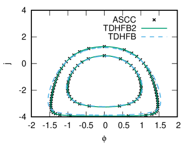
Figure 1: Classical trajectories satisfying the EBK quantization condition (2.17) with $k=1$ and 2 in the $(\phi,j)$ phase space. The crosses, solid and dashed lines correspond to the results of the ASCC+SPA, TDHFB2+SPA, and TDHFB+SPA, respectively. The crosses for the ASCC+SPA trajectories are plotted every ten calculations ($\delta q=10dq=0.1/\sqrt{\epsilon_{0}}$).

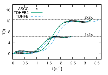
Figure 2: Calculated action integrals for the $\ket{0_{2}^{+}}$ and $\ket{0_{3}^{+}}$ states as functions of time $t$. The crosses, solid and dashed lines correspond to the ASCC+SPA, the TDHFB2+SPA, and the TDHFB+SPA, respectively. The action integrals are calculated on each trajectory in Fig. 1 from $(\phi,j)=(0,j_{\rm max})$ in the clockwise direction. The crosses for the ASCC+SPA trajectories are plotted every ten calculations ($\delta q=10dq=0.1/\sqrt{\epsilon_{0}}$).

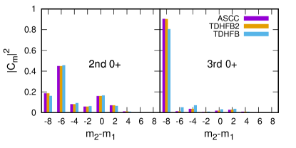
Figure 3: Occupation probabilities for the $0_{2}^{+}$ and $0_{3}^{+}$ states. The horizontal line indicates the $j=(m_{2}-m_{1})/2$ of the quasi-spin basis in Eq. (3.24). The vertical bars at each $m_{2}-m_{1}$ from left to right represent $|C_{m}|^{2}$ of Eq. (3.25) in the ASCC+SPA, TDHFB2+SPA and TDHFB+SPA calculations, respectively.

The two-level pairing model corresponds to the 2D TDHFB system. Explicitly separating the gauge angle $\Phi$ and fixing the particle number $J$, the 2D TDHFB is reduced to the 1D system with the relative angle $\phi\equiv\chi_{2}-\chi_{1}$ and the relative occupation $j\equiv(j_{2}-j_{1})/2$ as canonical variables. In Ref. Ni and Nakatsukasa (2018), using the explicit transformation to these separable variables, we examined the performance of the SPA requantization for the two-level model. In this section, we discuss the same model as in Ref. Ni and Nakatsukasa (2018), but we determine the transformation using the ASCC method and then apply the SPA (ASCC+SPA).

Here, we study the system with the equal degeneracy, $\Omega_{1}=\Omega_{2}=8$, the pairing strength $g/\epsilon_{0}=0.2$, and the particle number $N=16$. In this two-level case, we use the level spacing, $\epsilon_{0}\equiv\epsilon_{2}-\epsilon_{1}$, as the unit of energy. The moving-frame QRPA produces the zero mode and another eigenvector with a finite frequency squared $\omega^{2}\neq 0$. We follow the latter mode to construct the collective path. In the ASCC calculation, we set the increment of the collective coordinate, $dq=0.01$, in units of $1/\sqrt{\epsilon_{0}}$. We confirm that the pair rotation always has a zero frequency on the collective path. On the obtained collective path, we calculate a classical trajectory for the Hamiltonian

$$\mathcal{H}_{\rm coll}(q^{1},p_{1};J)=\frac{1}{2}p_{1}^{2}+V(q^{1},J)$$ (4.1)

with $J=N/2=8$. Calculated trajectories that satisfy the EBK quantization condition (2.17) for the first and second excited states ($0_{2}^{+}$ and $0_{3}^{+}$) are mapped onto the $(\phi,j)$ plane and shown in Fig. 1. We also calculate the trajectories using the explicit transformation of the variables to $(\Phi,J;\phi,j)$, which are shown by dashed lines in Fig. 1. We call this “TDHFB trajectories”. Small deviation in large $\phi$ is due to the absence of the higher-order terms in $\chi_{\alpha}$ in the ASCC. In fact, if we calculate the trajectories in the variables $(\Phi,J;\phi,j)$ using the Hamiltonian truncated up to the second order in $\chi_{\alpha}$ (“TDHFB2 trajectories”), we obtain the solid lines in Fig. 1, which perfectly agree with the ASCC trajectories.

The action integrals $\mathcal{T}(t)$ corresponding to these closed trajectories are shown in Fig. 2. For the $0_{2}^{+}$ state, all three calculations agree well with each other, while we see small deviation between the full TDHFB and the ASCC/TDHFB2 calculations for the $0_{3}^{+}$ state.

The calculated wave functions for the excited $0^{+}$ states are shown in Fig. 3. We show the occupation probabilities which are decomposed into the $2n$-particle-$2n$-hole components. The left end of the horizontal axis at $m_{2}-m_{1}=-8$ $(j=-4)$ corresponds to a state with $(m_{1},m_{2})=(N/2,0)$ where all the particles are in the lower level $\alpha=1$. The next one at $m_{2}-m_{1}=-6$ $(j=-3)$ corresponds to the one with $(m_{1},m_{2})=((N-2)/2,1)$, and so on. The results from the TDHFB2+SPA and the ASCC+SPA are identical to each other within numerical error, and they reproduce the TDHFB+SPA calculation well.

By comparing with the full TDHFB calculation with the ASCC+SPA approach in the two-level pairing model, we conclude that the ASCC is reliable for description of low-lying collective states, for which the adiabatic approximation is justifiable. In addition to that, we should note that the pair rotation is properly separated.

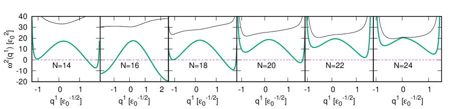
Figure 4: Eigenvalues of moving-frame QRPA equation as a function of the collective coordinate $q^{1}$, from $N=14$ to $N=24$. The thick (green) lines are the modes we choose as the collective coordinate $q^{1}$, while the dashed lines correspond to the zero modes ($q^{n}$). In each panel, both ends of the horizontal axis corresponds to the ending points of the collective path $q^{1}$.

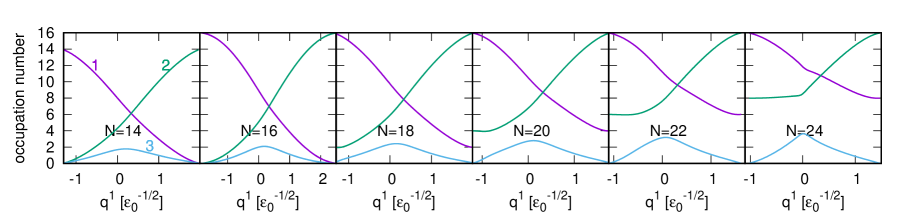
Figure 5: The occupation numbers $2j^{\alpha}$ in each single-particle level $\alpha$ as a function of the collective coordinate $q^{1}$, from $N=14$ to $N=24$. The purple, green, and blue lines correspond to $\alpha=1$, 2, and 3, respectively. At the left end point of the collective coordinate in each panel, the configuration corresponds to the “HF-like” states. See text for details.

IV.2 Non-integrable case (1): Three-level pairing model

In contrast to the two-level model, the TDHFB for the three-level model is non integrable. We set the parameters of the system as follows: $\Omega_{1}=\Omega_{2}=\Omega_{3}=\Omega=8$, $\epsilon_{1}=-\epsilon_{0}$, $\epsilon_{2}=0$, $\epsilon_{3}=1.5\epsilon_{0}$, and $g=0.2\epsilon_{0}$. We use the parameter $\epsilon_{0}$ as the unit energy. For the sub-shell closed configuration of $N=2\Omega=16$, the HFB ground state changes from the normal phase to the superfluid phase at $g_{c}=0.058\epsilon_{0}$. We calculate a chain of systems with even particle numbers from $N=14$ to $N=24$.

We obtain three eigen frequencies for the moving-frame QRPA equation, on the collective path (Fig. 4). First of all, we clearly identify the zero mode with $\omega^{2}=0$ everywhere along the collective path. This means that the pair rotation is separated from the other degrees of freedom in the ASCC. The frequency could become imaginary ($\omega^{2}<0$). Except for the case of sub-shell closure ($N=2\Omega_{1}=16$), the frequency rapidly increases near the end points. The end points are given by points where the search for the next point on the collective path in Sec. II.1 fails.

We choose the lowest frequency squared mode, except for the zero mode, as a generator of the collective path ($q^{1}$). Figure 5 shows variation of the occupation probability of each single-particle state, as functions of the collective coordinate $q^{1}$ on the collective path. The most striking feature is that the collective path terminates with special configurations which are given by the integer number of occupation. This is the reason why the search for the collective path fails at both the ends. At the end points, the occupation of the level 3 ($\epsilon_{3}$) vanishes, while those of the levels 1 and 2 become either maximum or minimum. The left end of each panel in Fig. 5 corresponds to a kind of “Hartree-Fock” (HF) state which minimizes the single-particle-energy sum, $\sum_{\alpha}2j_{\alpha}\epsilon_{\alpha}$. The pairing correlation is weakened in both ends of the collective path.

The collective mass with respect to the coordinate $q^{1}$ is normalized to unity. The collective potential is shown in Fig. 6. The range of $q^{1}$ is the largest for the system with $N=16$. This is because the variation of $j^{1}$ and $j^{2}$ is the largest in this case.

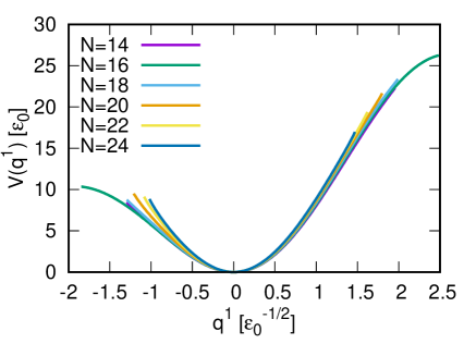
Figure 6: Collective potential $V(q^{1})$ obtained from the ASCC. We adjust the energy minimum point as $q^{1}=0$ and $V=0$.

Table 1: Calculated excitation energies of the first and the second excited states in units of $\epsilon_{0}$. In the exact calculation, the second excited state in the ASCC+SPA corresponds to the $0_{4}^{+}$ state. See text for details.

$N$	$14$	$16$	$18$	$20$	$22$	$24$
ASCC+SPA (1st exc.)	$3.87$	$3.90$	$3.97$	$4.09$	$4.23$	$4.33$
Exact	$4.09$	$4.13$	$4.20$	$4.30$	$4.44$	$4.60$
ASCC+SPA (2nd exc.)	$7.42$	$7.42$	$7.60$	$7.92$	$8.26$	$8.47$
Exact	$7.65$	$7.71$	$7.88$	$8.15$	$8.49$	$8.74$

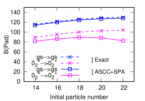
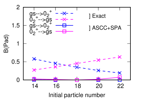
Figure 7: Calculated strength of pair-addition transition (4.2) from $N=14$ to $N=22$. The solid (dashed) lines correspond to the ASCC+SPA (exact) calculation. The horizontal line indicates the particle number of the initial states. The upper panel shows the intraband transitions, $0_{1}^{+}\to 0_{1}^{+}$ and $0_{2}^{+}\to 0_{2}^{+}$, while the lower panel shows the interband transitions, $0_{1}^{+}\to 0_{2}^{+}$ and $0_{2}^{+}\to 0_{1}^{+}$.

Based on the collective path determined by the ASCC calculation, we perform the requantization according to the SPA. Table 1 shows the excitation energies of the first and second excited states, determined by the EBK quantization condition (2.17). Comparing the result of the ASCC+SPA with that of the exact calculation, we find that the excitation energies are reasonably well reproduced. The ASCC+SPA underestimates the excitation energies only by about 5 %.

It should be noted that the second excited state in the collective path corresponds to the $0_{4}^{+}$ state, not to the $0_{3}^{+}$ state, in the exact calculation. We examine the interband $(k\neq k^{\prime})$ pair-addition transition,

$$B(P_{\rm ad};k\rightarrow k^{\prime})\equiv\left|\bra{0_{k^{\prime}}^{+};N+2}\hat{S}^{+}\ket{0_{k}^{+};N}\right|^{2},$$ (4.2)

in the exact solution. $B(P_{\rm ad};0_{2}^{+}\rightarrow 0_{3}^{+})$ is $10\sim 100$ times smaller than $B(P_{\rm ad};0_{1}^{+}\rightarrow 0_{3}^{+})$, while $B(P_{\rm ad};0_{1}^{+}\rightarrow 0_{2}^{+})$ and $B(P_{\rm ad};0_{1}^{+}\rightarrow 0_{3}^{+})$ are in the same order. The ASCC+SPA produces states in the same family, namely, those belonging to the same collective subspace (path). In the phonon-like picture, we expect similar magnitude of the strengths for $B(P_{\rm ad};{\rm g.s.}\rightarrow\omega_{\rm phon})$ and $B(P_{\rm ad};\omega_{\rm phon}\rightarrow 2\omega_{\rm phon})$, but smaller values of $B(P_{\rm ad};{\rm g.s.}\rightarrow 2\omega_{\rm phon})$. Thus, the $0_{4}^{+}$ state in the exact calculation corresponds to the two-phonon state in the ASCC+SPA. The $0_{3}^{+}$ state in the exact calculation may correspond to a collective path associated with another solution of the moving-frame QRPA (thin black line in Fig. 4).

Next, we calculate the wave functions, according to Eqs. (3.24) and (3.26). The ground state corresponds to the number-projected HFB state (variation before projection). In contrast, the excited states are given as superposition of generalized Slater determinants in the collective subspace, The pair-addition transition strengths computed using these wave functions of the excited states are shown in Fig. 7. For the intraband transition ($k=k^{\prime}$ in Eq. (4.2)), the ASCC+SPA method well reproduces the strengths of the exact calculation. The ground-to-ground transitions, $B(P_{\rm ad};0_{1}^{+}\rightarrow 0_{1}^{+})$, are perfectly reproduced, while $B(P_{\rm ad};0_{2}^{+}\rightarrow 0_{2}^{+})$ are underestimated by about $10\%\sim 20\%$.

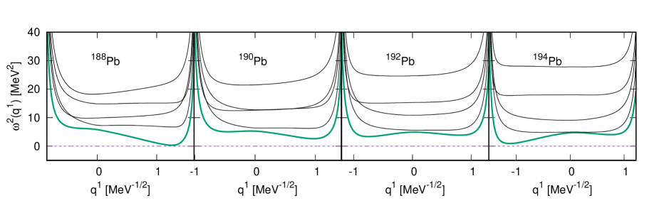
Figure 8: The same as Fig. 4 but for Pb isotopes.

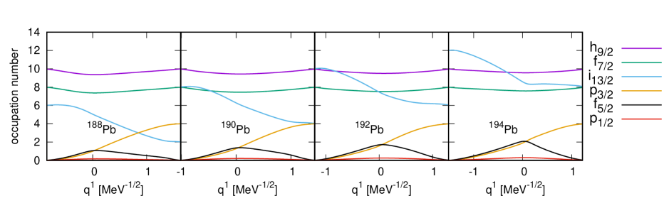
Figure 9: The same as Fig. 5 but for Pb isotopes.

It is more difficult to reproduce the absolute magnitude of interband transitions ($k\neq k^{\prime}$), which are far smaller than the intraband transitions. Although the increasing (decreasing) trend for $B(P_{\rm ad};0_{2}^{+}\rightarrow 0_{1}^{+})$ ($B(P_{\rm ad};0_{1}^{+}\rightarrow 0_{2}^{+})$) as a function of the particle number is properly reproduced, the absolute magnitude is significantly underestimated in the ASCC+SPA. This is due to extremely small collectivity in the interband transitions. Almost all the strengths are absorbed in the intraband transitions. Even in the exact calculation, the pair addition strength is about two orders of magnitude smaller than the intraband strength. Remember that the non-collective limit ($g\rightarrow 0$) of this value is $B(P_{\rm ad};0_{1}^{+}\rightarrow 0_{2}^{+})=\Omega$. Therefore, the pairing correlation hinders the interband transitions by about one order of magnitude. For such tiny quantities, perhaps, the reduction to the 1D collective path is not well justified.

We should remark here that there is a difficulty in the present ASCC+SPA requantization for weak pairing cases. In such cases, the potential minimum is close to the left end ($q^{1}=q_{L}$) of the collective path, and the potential height at $q^{1}=q_{L}$, $V(q_{L})-V(0)$, becomes small. Then, a classical trajectory with $E>V(q_{L})$ hits this boundary ($q^{1}=q_{L}$). In construction of wave functions, the boundary condition at $q^{1}=q_{L}$ significantly influences the result. In the present study, we choose a strong pairing case to avoid such a situation. As in Fig. 6, the potential height at $q^{1}=q_{L}$ has about $10\epsilon_{0}$ which is larger than the excitation energies of the second excitation. Therefore, all the trajectories are “closed” in the usual sense.

IV.3 Non-integrable case (2): Pb isotopes

Finally, we apply our method to neutrons’ pairing dynamics in neutron-deficient Pb isotopes. The spherical single-particle levels of neutrons between the magic numbers 82 and 126 are adopted and their energies are presented in Table 2. The coupling constant $g=0.138$ MeV is determined to reproduce the experimental pairing gap given by the odd-even mass difference, $\Delta(N)=\frac{(-1)^{N+1}}{2}[B(N+1)-2B(N)+B(N-1)]$ of ¹⁹²Pb. The even-even nuclei from ¹⁸⁸Pb to ¹⁹⁴Pb are studied.

Table 2: Single-particle energies of Pb isotopes used in the calculation in units of MeV. These are obtained from the spherical Woods-Saxon potential with the parameters of Ref. Bohr and Mottelson (1969).

orbit	$h_{9/2}$	$f_{7/2}$	$i_{13/2}$	$p_{3/2}$	$f_{5/2}$	$p_{1/2}$
energy(MeV)	$-10.94$	$-10.69$	$-8.74$	$-8.44$	$-8.16$	$-7.45$

The TDHFB dynamics is described by six degrees of freedom. Figure 8 shows eigenvalues of the moving-frame QRPA equation. Again, we find that there is a zero mode corresponding to the neutron pair rotation. Among the five vibrational modes, we choose the lowest one to construct the collective path in the ASCC. This lowest mode never crosses with other modes, though the spacing between the lowest to the next lowest mode can be very small, especially for ¹⁹⁴Pb. The evolution of the occupation numbers along the collective path is shown in Fig. 9. Similarly to the three-level model, the end points of the collective path indicate exactly the integer numbers, and the left end of each panel corresponds to the “Hartree-Fock”-like state. On the collective path, the occupation numbers of $i_{13/2}$, $p_{3/2}$, and $f_{5/2}$ mainly change.

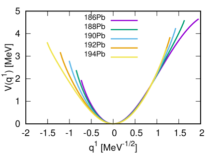
Figure 10: The same as Fig. 6 but for Pb isotopes.

The collective potentials for these isotopes are shown in Fig. 10. The heights of the potentials at the left end, $V(q_{L})-V(0)$, are $2\sim 3.5$ MeV. For ¹⁸⁶Pb, the height of the potential is not enough to satisfy the condition, $E<V(q_{L})$, to have a closed trajectory for the first excited state (See the last paragraph in Sec. IV.2). We encounter another kind of problem for ¹⁹⁶Pb, which will be discussed in Sec. V. Therefore, in this paper, we calculate the first excited states in ^{188,190,192,194}Pb.

We show the calculated excitation energy of the first excited state in Table 3. Experimentally, this pair vibrational excited $0^{+}$ state is fragmented into several $0^{+}$ states due to other correlations, such as quadrupole correlation, not taken into account in the present model. We make a comparison with the exact solution of the multi-level pairing model. The ASCC+SPA method quantitatively reproduces the excitation energy of the exact solution.

Table 3: The same as Table 1 but for Pb isotopes. The energies are given in units of MeV.

	186Pb	188Pb	190Pb	192Pb	194Pb	196Pb
ASCC+SPA	$-$	$2.31$	$2.21$	$2.12$	$2.04$	$-$
Exact	$2.58$	$2.44$	$2.34$	$2.25$	$2.20$	$2.15$

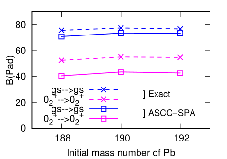
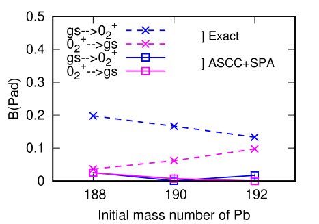
Figure 11: The same as Fig. 7 but for Pb isotopes.

The pair-addition transition strengths are shown in Fig. 11. The feature that is similar to the three-level case is observed: dominant intraband transition and very weak interband transitions. The accuracy from the ASCC+SPA method well reproduces $B(P_{\rm ad};0_{1}^{+}\rightarrow 0_{1}^{+})$ and qualitatively reproduces $B(P_{\rm ad};0_{2}^{+}\rightarrow 0_{2}^{+})$ as well. The deviation for the latter is about $25\%$. The interband transitions are smaller than the intraband transitions by more than two orders of magnitude. This is also similar to the three-level model discussed in Sec. IV.2. For such weak transitions, the ASCC+SPA significantly underestimates the strengths. We may say that the ASCC+SPA gives reasonable results for the intraband transitions in the realistic values of the pairing coupling constant $g$ and single-particle levels.

Finally, we discuss the validity of the collective model approach assuming the pairing gap as a collective coordinate. The 5D collective Hamiltonian assuming the quadrupole deformation parameters $\alpha_{2\mu}(\mu=\pm 2,\pm 1,$ and $0)$ as the collective coordinates is widely utilized to analyze experimental data of quadrupole states. Similarly, we may construct the pairing collective Hamiltonian in terms of the pairing gap $\Delta$ and the gauge angle $\Phi$. As far as there is a one-to-one correspondence between $\Delta$ and the collective variable $q^{1}$ we obtained in the present study, we can transform the collective Hamiltonian in $(q^{1},\Phi)$ into the one in $(\Delta,\Phi)$. The pairing gap $\Delta$ is defined as

$$\Delta(q) \equiv\left.g\braket{\Phi,J;q,p}{\hat{S}^{-}}{\Phi,J;q,p}\right|_{\Phi=p=0}$$

$$=g\sum_{\alpha}\sqrt{j^{\alpha}(\Omega_{\alpha}-j^{\alpha})}.$$ (4.3)

Figure 12 shows the pairing gap $\Delta$ in ¹⁹²Pb as a function of the collective coordinate $q^{1}$. The peak in $\Delta$ is near $q^{1}=0$ and it is not a monotonic function of $q^{1}$, thus no one-to-one correspondence exists. The same behavior is observed for other Pb isotopes too. Therefore, the pairing gap $\Delta$ is not a suitable collective coordinate to describe the pairing dynamics in the multi-level model.

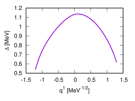
Figure 12: Pairing gap as a function of collective coordinate $q^{1}$ in ¹⁹²Pb.

V Conclusion and discussion

Extending our former work Ni and Nakatsukasa (2018), which demonstrated the accuracy of the SPA for the requantization of the TDHFB dynamics in the two-level pairing model, we propose the ASCC+SPA method for non-integrable systems. In this approach, we use the ASCC method to extract the 2D collective subspace including the pair rotation. In other words, we extract an approximate integrable system in the non-integrable system described by $(q^{1},p_{1};J,\Phi)$.

We apply the ASCC+SPA method to the multi-level pairing model. We investigate the three-level model and the multi-level model simulating Pb isotopes with a realistic pairing coupling constant $g$ and single-particle levels. In both cases, the low-lying excited $0^{+}$ states obtained with the ASCC+SPA well reproduce the exact solutions not only of the excitation energies but also of the wave functions. In the ASCC+SPA, the pair-transition calculation is straightforward, because we have a microscopic wave function for every quantized state. This overcomes a disadvantage in the conventional canonical requantization in which we need to construct a pair-transition operator in terms of the collective variables only.

Although the overall agreement between the ASCC+SPA and the exact calculations is good in general, we have encountered several problems remaining to be solved. First, we can calculate a classical trajectory bound by the pocket of a potential. However, it is not trivial how to treat “unbound” trajectories that hit the end point of the collective path. See the potentials in Figs. 6 and 10. This happens in the calculation of ¹⁸⁶Pb (Sec. IV.3). Probably, it is necessary to find a proper boundary condition in the collective subspace. For instance, the 5D quadrupole collective model has such boundary conditions imposed by the symmetry property of the quadrupole degrees of freedom Kumar and Baranger (1967).

The second problem occurred in the calculation of ¹⁹⁶Pb, in which we have encountered complex eigenvalues and eigenvectors of the moving-frame QRPA equation. This happens at a point where the two eigen frequencies become identical, $\omega_{1}^{2}=\omega_{2}^{2}$, namely at a crossing point. We do not have a problem for the crossing between the pair rotational mode and the other modes. Currently, we do not know exactly when the complex solutions emerge.

Another problem we need to solve is a description of the quantum tunneling. The tunneling plays an essential role in spontaneous fission, sub-barrier fusion reaction, and shape coexistence phenomena Nakatsukasa et al. (2016); Wen and Nakatsukasa (2016, 2017); Hinohara et al. (2007, 2008). In the present ASCC+SPA, the classical trajectory cannot penetrate the potential barrier. Since the ASCC is able to provide the 1D collective coordinate, the imaginary-time TDHF is feasible and may be a solution to this problem Negele (1982). These remaining issues in the ASCC+SPA approach should be addressed in future.