Astigmatic tomography of orbital angular momentum superpositions

Abstract

We use astigmatic transformations to characterize two-dimensional superpositions of Orbital Angular Momentum (OAM) states in laser beams. We propose two methods for doing this, both relying only on astigmatic transformations, viewed as rotations on the Poincaré sphere, followed by imaging. These methods can be used as a tomographic tool for communication protocols based on optical vortices.

I introduction

The orbital angular momentum (OAM) of light has been used for numerous applications, including optical tweezing tweezer1 ; tweezer2 and communication protocols cryptouff ; cryptolorenzo ; tamburini ; krenn . The ability to generate and detect OAM beams has become imperative for such applications oam25 . The demonstration of OAM entanglement in photon pairs generated by spontaneous parametric down conversion has brought OAM into the experimental toolbox of quantum information zeilinger . Nowadays, several methods for generating, transforming and detecting OAM beams can be found in the literature oam-masurement1 ; oam-masurement2 ; oam-sorter1 ; Schlederer16 ; oam-sorter2 ; oam-electron . The astigmatic mode conversion is a powerful tool and has been widely used for implementing unitary transformations in the OAM degree of freedom. The astigmatic effect can be introduced either by cylindrical lenses woerdman ; kimel ; cnotuff or by tilted spherical lenses tilted .

The formal equivalence between first order paraxial modes and light polarization naturally leads to a Poincaré sphere representation of these modes and their use as an additional qubit for quantum information encoding poincare . In this way, two qubits can be encoded in a single photon, one on its polarization state and the other on its OAM structure topoluff ; quplate ; cardano ; leo1 ; milione ; aiello2 ; structured-waves . One central issue in quantum information processing is the characterization of a qubit source, determining the quantum state it produces. The most common approach allowing the tomographic reconstruction of the transverse spatial state of paraxial light fields employs projective measurements based on the phase-flattening of the field wavefront Giovannini13 ; Qassim14 ; Rathore17 . More recently, wavefront reconstruction methods exploring digital holography DErrico17 ; Knudsen17 have also been used to characterize the transverse spatial state in terms of its OAM constituents.

In this work we exploit the astigmatic effect to measure arbitrary superpositions of OAM superpositions. We provide two distinct experimental demonstrations of the use of astigmatic optical elements to obtain the spherical coordinates of first order OAM modes in the Poincaré sphere. Our methods can be geometrically interpreted in terms of rotations in the sphere and require at most three images of the astigmatically-transformed beam under investigation. We demonstrate these methods with beams prepared in two-dimensional superpositions of OAM states with topological charges $\pm 1\,$, but their extension to two-dimensional superpositions of higher topological charges $\pm l$ $(l>1)$ is straightforward.

The paper is structured as follows. In section II we briefly review the mathematical representation of astigmatic transformations. In section III we describe a simple tomographic method based on the visibility maximization of the astigmatically transformed beam. This visibility is maximized over a continuous parameter (an angle) of the astigmatic transformations. Our experimental scheme and supporting experimental results are presented in section III.1. In section IV we describe a second tomographic method utilizing a fixed number ($\leqslant$ 2) of astigmatic transformations and test it with our experimental data. Conclusions are presented in section V.

II Review: astigmatic transformations on the Poincaré sphere

In this section we review how optical vortices with Orbital Angular Momentum (OAM) topological charge $\pm 1$ can be pictured on the Poincaré sphere. We also describe astigmatic transformations on these states as rotations of the Poincaré sphere. Later, in sections III and IV, we describe two different ways to characterise general states on the Poincaré sphere using only astigmatic transformations and the orientation of the resulting HG modes, obtained by imaging.

Pure vortex beams are characterized by a rotationally symmetric intensity distribution around the propagation axis accompanied by the azimuthal variation of the phase. This makes it difficult to measure the topological charge of an optical vortex with intensity only measurements. In general one must resort to interferometry in order to resolve the azimuthal phase variation DErrico17 ; Knudsen17 . However, the astigmatic mode conversion can transform pure Laguerre-Gaussian (LG) beams into Hermite-Gaussian (HG) intensity distributions that can be directly identified through intensity measurements. For example, the astigmatic effect provided by a spherical tilted lens has been used as a tool for topological charge measurements tilted . Rather than simply measuring the topological charge, the ability to resolve OAM superpositions is a much more difficult task. Resolution of the superposition constituents, their weights and relative phases cannot be easily measured at once.

However, if we restrict the OAM degree of freedom to a two-dimensional subspace, it is possible to use astigmatic transformations to resolve arbitrary superpositions with intensity only measurements. In this work we manipulate arbitrary superpositions of two OAM beams with opposite topological charges $\pm 1\,$,

$$\psi_{\theta,\phi}(\mathbf{r}) = \cos\left(\frac{\theta}{2}\right)\,LG_{+}(\mathbf{r})+e^{i\phi}\sin\left(\frac{\theta}{2}\right)\,LG_{-}(\mathbf{r})\,,$$

where $LG_{\pm}$ is the Laguerre-Gaussian mode function with topological charge $\pm 1\,$, $\mathbf{r}$ is the transverse position and $\theta$ and $\phi$ are, respectively, the sagittal and azimuthal angles in the Poincaré sphere representation. This general superposition can be formally represented as the column vector

$$\lvert\theta,\phi\rangle = \left[\begin{matrix}\cos\frac{\theta}{2}\\ e^{i\phi}\sin\frac{\theta}{2}\\ \end{matrix}\right]\;.$$ (2)

This two-dimensional complex vector space is analogous to the Hilbert space of a two-level system, a qubit. Accordingly, there is a one-to-one correspondence between each state (2) and points on the surface of the Poincaré sphere (see Fig. 1-a).

Figure 1: a) Poincaré sphere epresentation of the two-dimensional space of Orbital Angular Momentum topological charge $\pm 1$. b) The astigmatic transformations we apply correspond to rotations on the Poincaré sphere, by angle $-\pi/2$ around an axis on the equator. Here we picture one such rotation which does not map the initial point to the equator (red), and one which does (blue).

The action of an astigmatic mode converter is conveniently represented using this matrix formulation. An LG-HG mode converter rotated by $\beta/2$ with respect to the horizontal introduces a $\pi/2$ retardation between HG modes oriented at $\beta/2$ and $(\beta+\pi)/2\,$. This is naturally represented by

$$MC(\beta) = \left\lvert\frac{\pi}{2},\beta\right\rangle\left\langle\frac{\pi}{2},\beta\right\rvert-i\left\lvert\frac{\pi}{2},\beta+\pi\right\rangle\left\langle\frac{\pi}{2},\beta+\pi\right\rvert$$ (3)

$$= \frac{e^{i\pi/4}}{\sqrt{2}}\left[\begin{matrix}1&i\,e^{-i\beta}\\ i\,e^{i\beta}&1\\ \end{matrix}\right]\;.$$

This transformation is a good approximation to the one implemented either by a LG-HG mode converter, or by a tilted spherical lens, as proposed in tilted . Geometrically, this is a rotation by an angle $-\pi/2$ around an axis on the equator of the Poincaré sphere, situated at angle $\beta$ with the $x$ axis (see Fig. 1-b).

In the next section we describe our first method to characterize arbitrary superpositions of first order OAM modes on the Poincaré sphere.

III Method I: Hermite-Gaussian mode visibility

As we have seen in the previous section, an astigmatic LG-HG mode converter rotates states by $-\pi/2$ radians around an axis in the equator of the Poincaré sphere. The orientation of the rotation axis with respect to the $x$ axis is given by $\beta$, where $\beta/2$ is the physical angle of the LG-HG mode converter with respect to the horizontal.

It is a geometrical fact that any point (A) on a sphere is mapped to some point (C) on the equator by a $\pi/2$ rotation around a suitable axis on the equator (see the blue arc in Fig. 1-b). Thus, for any state on the Poincaré sphere, there must be a LG-HG mode converter orientation that takes the state onto the equator. Points on the equator correspond to rotated HG modes which can be easily identified from intensity measurements (images) only.

After passing through the mode converter, the general superposition (2) is transformed into

$$MC(\beta)\lvert\theta,\phi\rangle = \frac{e^{i\pi/4}}{\sqrt{2}}\left[\begin{matrix}\cos\frac{\theta}{2}+i\,e^{i(\phi-\beta)}\sin\frac{\theta}{2}\\ \\ i\,e^{i\beta}\cos\frac{\theta}{2}+\,e^{i\phi}\sin\frac{\theta}{2}\\ \end{matrix}\right]\;.$$ (4)

Our first method to determine the transverse mode state involves rotating the mode converter until we find the appropriate angle $\beta$ for which the general mode (2) can be recognised by imaging as a rotated HG mode. In this case, the two column entries must have the same absolute values

$$\left\lvert\cos\frac{\theta}{2}+i\,e^{i(\phi-\beta)}\sin\frac{\theta}{2}\right\rvert = \left\lvert i\,e^{i\beta}\cos\frac{\theta}{2}+\,e^{i\phi}\sin\frac{\theta}{2}\right\rvert\;.$$

(5)

Of course, this condition is naturally fulfilled for $\theta=0$ or $\pi\,$, regardless to the value of $\beta$ (pure LG modes are transformed into HG modes for any orientation of the mode converter). For arbitrary $\theta\,$, condition (5) brings us to

$$\beta_{MC} = \phi\;.$$ (6)

The orientation of the resulting HG mode with respect to the horizontal is given by

$$\alpha_{HG} = \frac{1}{2}\arg\left(\frac{i\,e^{i\beta}\cos\frac{\theta}{2}+\,e^{i\phi}\sin\frac{\theta}{2}}{\cos\frac{\theta}{2}+i\,e^{i(\phi-\beta)}\sin\frac{\theta}{2}}\right)$$ (7)

$$= \frac{\phi-\theta}{2}+45^{\circ}\,.$$

Therefore, an arbitrary superposition can be characterized by two angles. The first is the mode converter orientation $\beta_{MC}/2\,$ with respect to the horizontal, which takes the superposition into a rotated HG mode. The second angle is the resulting orientation $\alpha_{HG}\,$ of the HG mode found in this way.

III.1 Experimental implementation

In order to apply the result of the previous section, we start by preparing various superpositions of $LG_{\pm}$ modes, sending them through an astigmatic analyzer. The superposition parameters $(\theta,\phi)$ are then inferred from the measured values of $\beta_{MC}$ and $\alpha_{HG}$ according to Eqs. (6) and (7).

The experimental setup is depicted in Fig. 2. The Gaussian beam from a He-Ne laser ($\lambda=633nm$) is sent to one half of a reflective spatial light modulator (SLM) panel, programmed to create a controllable OAM state $\lvert\theta,\phi\rangle\,$. Then, the astigmatic analyzer is implemented in the other half of the SLM, programmed with a phase modulation that emulates the transmission function of a tilted lens tilted . A charge coupled device (CCD) camera positioned close to the focal plane of this tilted lens is used to acquire the image of the transformed beam. Two parameters are set by the analyzer: the tilt angle $\xi\,$, which remains fixed once calibrated, and the angle $\beta/2$, as shown in Fig. 3. The astigmatic phase profile written on the SLM is provided in appendix A.

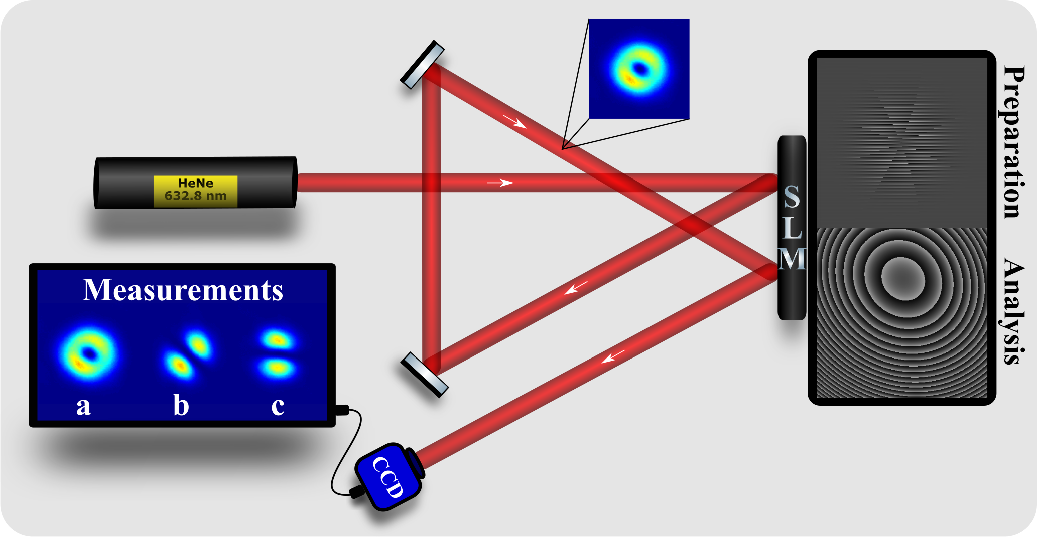
Figure 2: Experimental setup. The screen of the SLM was split in two sides, one for the preparation of the mode and the other to emulate the tilted lens. The screen connected to the CCD shows the three images used in the method II, these images are not captured simultaneously.

Figure 3: Tilted lens orientation. A spherical lens (axis $\mathbf{\hat{n}}$) implements the astigmatic mode conversion given by Eq. (3). The tilt angle $\xi$ is determined experimentally, so that a rotation of $-\pi/2$ radians on the Poincaré sphere is achieved. The axis of the rotation on the Poincaré sphere is on its equator, at an angle $\beta$ with the $x$ axis, determined by the angle of the projection of $\mathbf{\hat{n}}$ with the transverse plane, as in the figure.

First, the tilt angle is calibrated by sending a pure LG beam to the SLM analyzer and verifying the correct formation of a pure HG profile close to the focal plane, as described in Ref. tilted . This calibration is independent of the lens axis orientation, which is initially placed at the horizontal plane. Once calibration is achieved, the analyzer is ready to receive the sample OAM states. The analysis is performed by keeping fixed the tilt angle and turning the lens axis $\mathbf{\hat{n}}$ around the beam propagation direction until a pure HG profile is found in the observation plane. At this moment, we take note of two angles: the orientation $\beta_{MC}/2$ of the transverse projection of the lens axis $\mathbf{\hat{n}}$ with respect to the $x^{\prime}$ axis (see Fig. 3), and the orientation $\alpha_{HG}$ of the line connecting the maxima of the resulting HG mode, with respect to the horizontal (see appendix B). According to Eqs. (6) and (7), they determine the Poincaré sphere coordinates $(\theta,\phi)$ of the sample state.

The astigmatic mode analysis has been tested with two sequences of sample states, as represented in Fig. 4. The first sequence (A-E) covers the path along the meridian $\phi=0$ and illustrates the relationship between $\alpha_{HG}$ and $\theta\,$. In Fig. 5a we show the input modes produced by the preparation screen and the resulting HG profiles at the output of the analyzer. The graphical representation of $\alpha_{HG}$ versus $\theta$ is presented in Fig. 5b.

Figure 4: Poincaré sphere representation of the sample modes used for testing the astigmatic analyzer.

Figure 5: a) Images of the input modes and the resulting outputs from the astigmatic analyzer for the sequence A-E. b) Graphical representation of the measured orientations $\alpha_{HG}$ versus $\theta\,$. Blue dots are the experimental results and red solid line is the theoretical prediction given by Eq. (7).

The second sequence (D1-D8) covers the path along the polar circle $\theta=135^{\circ}$ and illustrates the relationship between $\alpha_{HG}$ and $\phi\,$. In Fig. 6a we show the input modes produced by the preparation screen and the resulting HG profiles at the output of the analyzer. The graphical representation of $\alpha_{HG}$ versus $\phi$ is presented in Fig. 6b.

Figure 6: a) Images of the input modes and the resulting outputs from the astigmatic analyzer for the sequence D1-D8. b) Graphical representation of the measured orientations $\alpha_{HG}$ versus $\phi\,$. Blue dots are the experimental results and red solid line is the theoretical prediction given by Eq. (7).

The graphs presented in Figs. 5 and 6 show a good agreement between the experimental results and the theoretical expression (7). Errors due to the experimental determination of $\beta_{MC}$ and $\alpha_{HG}$ are propagated and expressed as error bars. The average errors achieved with this method are $\Delta\theta=12^{\circ}$ and $\Delta\phi=10^{\circ}$. These errors are relatively large. In the next section we describe a second method that also uses astigmatic transformations and imaging to obtain a more precise determination of the transverse mode state.

IV Method II: Poincaré sphere positioning

Of course, pure intensity measurements alone cannot provide full information about arbitrary OAM superpositions. However, partial information can be obtained by measuring the intensity distribution and the orientation $\alpha$ of the line connecting the two intensity maxima (with respect to the horizontal). This gives the azimuthal coordinate $\phi=2\alpha$ of the mode superposition in question. Therefore, from pure intensity measurements we determine the meridian line, in the Poincaré sphere, passing through the point representing the state. Note, however, that the image of states too close to the poles on the $z$ axis will present low visibility of the maxima, as the states are close to LG states, for which the intensity distribution is symmetrical around the center. We should treat these polar regions as blind spots for our longitude determination; they will be discriminated by other measurements, as we now describe.

As we have seen, the astigmatic mode conversion can be geometrically interpreted as a $-\pi/2$ rotation of the Poincaré sphere around the axis connecting the mode conversion eigenstates. For example, a horizontal mode converter (eigenstates $\lvert\pi/2,0\rangle$ and $\lvert\pi/2,\pi\rangle$) rotates states by $-\pi/2$ radians around the $x$ axis, mapping all states on the meridians $\phi=0$ and $\phi=\pi$ onto the equator.

Our strategy for finding the position of states on the Poincaré sphere requires determining the orientation $\alpha$ with respect to the horizontal of the two maxima in three images for each state we would like to characterise. The first is the direct image without mode conversion ($\alpha_{NL}$); the second ($\alpha_{0^{\circ}}$), after a transformation corresponding to a horizontal LG-HG mode converter ($\beta/2=0$); an the third ($\alpha_{45^{\circ}}$), after a mode converter oriented at $\beta/2=45^{\circ}$. As can be seen in Fig. 7-a, each measurement will have low visibility for states in one of the six polar blind spots.

Figure 7: a) The spherical caps in blue, around the $x,y$ and $z$ axes, represent states for which one of the three images will have a mode with low visibility. Due to this, we will call theses caps polar blind-spots. States in each cap will be determined from the two images which has modes with good visibility. b) States near the three pictured great circles will result in an intersection between halves of great circles which corresponds to a very narrow triangle (see Fig. 9-a). These will be obtained as the mid-point of the shortest triangle side (see Fig. 9-a).

Ideally, this gives the input state as the intersection between three halves of great circles intersecting the $x,y$ and $z$ axes, as depicted in Fig. 8. Note that states on the $xy,xz,yz$ planes, i.e. on precisely the three great circles in Fig. 7-b, are particular with respect to this characterization. This is because they sit on an overlap between two halves of great circles, and this overlap has a length of a quarter of a great circle. This means states will fail to be characterised as the intersection of two halves of great circles, hence the need for three images. Using the three images also guarantees that the polar, low-visibility “blind spots” can always be avoided, as each of the six polar spots in Fig. 7-a is only blind to a single measurement; in these cases, the two remaining measurements provide an intersection of two halves of a great circle, which determine the state’s position.

Figure 8: Poincaré representation of the three-measurement scheme. Characterisation of the angle that the line connecting the maxima makes with the horizontal gives information about the $z$- axis longitude (green). By previously rotating the Poincaré sphere via two astigmatic transformations, the same imaging technique gives us the $x$-axis longitude (blue) and $y$-axis longitude (red). In an idealized measurement, the three longitudes would intersect at the point representing the state.

IV.1 Experimental implementation

The experimental scheme is as described in section III.1, please see Fig. 2. We experimentally tested the method with the twenty six sample states represented by the red dots in Fig. 10. Three orientations ($\alpha_{NL},\alpha_{0^{\circ}},\alpha_{45^{\circ}}$) of the maxima with respect to the horizontal were measured for each sample state and the state’s parameters were estimated from the intersection between the three half great-circles inferred from each measurement. Due to experimental imperfections, we did not obtain a single intersection, but three corners of a triangular region on the Poincaré sphere.

For each point, we first test whether we are in one of the six polar blind spots of Fig. 7-a. This was done by checking the visibility of each of the three images (see appendix B). A straighforward theoretical calculation determines that a minimum threshold of $v\leq 0.34$ determines a polar cap of 0.38 steradians, as in Fig. 7-a. In the cases when a point has a visibility below the threshold (i.e. is within a blind polar cap), we ignore the corresponding measurement/image, and the point’s coordinates are determined by the intersection of the two halves of great circles corresponding to the other two measurements.

Next, we experimentally evaluate whether the state is on, or near, the problematic great circles whose axes are the $x,y$ and $z$ axes (see Fig. 7-b). This was done by comparing the sides of the triangular region determined by the three halves of great circles (see Fig. 9): if the shortest triangle side was shorter than half of the next shortest side, we considered the state was too close to one of the problematic great circles. In these cases, we estimated the state as lying on the mid-point of the shortest triangle side (see Fig. 9-a). The distance between two vertices of the triangle can be obtained from their scalar product. Given that the vertices are on the surface of the Poincaré sphere with unit radius, the distance is simply given by

$$\mathrm{Dist}_{ab}=\arccos(\textbf{a}\cdot\textbf{b}),$$ (8)

where a and b are vectors that point to the vertices of the triangle.

Figure 9: a) A state will be deemed near to the three problematic great circles of Fig. 7-b when the three determined longitudes determine a narrow triangle (with shortest side smaller than half the next shortest side, in blue). In this case, we estimate the state as being at the half-point of the shortest side. b) For generic states, far from the polar caps of Fig. 7-a and the great circles of Fig. 7-b, the state is deemed to be at the center of the spherical triangle (in blue).

Let us assume now that the state is generic, i.e. it is both far from the blind polar regions of Fig. 7-a, and from the problematic great circles of Fig. 7-b. Then we estimate the state’s parameters to be at the center of the triangular region determined by the three intersections of halves of great circles (see Fig. 9-b), with error bars given by the largest variations of the state parameters within the triangular region.

Figure 10: Poincaré representation of the sample states used to test the three-measurement scheme.

In table 1 we show our experimental results. We also calculated the fidelity between the measured and the target states, which evaluates the overall efficiency of the preparation and analysis process. The average error in determination of the angles was $\Delta\theta=5^{\circ}$ and $\Delta\phi=2^{\circ}$, while the average fidelity was $0.992\pm 0.003$.

Point	$\theta_{T}$	$\phi_{T}$	$\theta_{E}\pm\Delta\theta_{E}$	$\phi_{E}\pm\Delta\phi_{E}$	Fidelity
1	0º	0º	4º$\pm$ 2º	121º$\pm$ 0º	0.999 $\pm$ 0.001
2	45º	0º	41º$\pm$ 2º	359º$\pm$ 5º	0.999 $\pm$ 0.001
3	90º	0º	88º$\pm$ 2º	354º$\pm$ 1º	0.997 $\pm$ 0.001
4	135º	0º	140º$\pm$ 2º	346º$\pm$ 1º	0.991 $\pm$ 0.002
5	180º	0º	166º$\pm$ 2º	270º$\pm$ 0º	0.986 $\pm$ 0.004
6	45º	45º	47º$\pm$ 10º	46º$\pm$ 6º	0.999 $\pm$ 0.003
7	90º	45º	94º$\pm$ 14º	36º$\pm$ 1º	0.993 $\pm$ 0.009
8	135º	45º	145º$\pm$ 2º	28º$\pm$ 1º	0.983 $\pm$ 0.003
9	45º	90º	52º$\pm$ 2º	83º$\pm$ 4º	0.994 $\pm$ 0.003
10	90º	90º	102º$\pm$ 2º	83º$\pm$ 1º	0.985 $\pm$ 0.003
11	135º	90º	152º$\pm$ 2º	91º$\pm$ 4º	0.979 $\pm$ 0.005
12	45º	135º	44º$\pm$ 10º	125º$\pm$ 5º	0.997 $\pm$ 0.004
13	90º	135º	89º$\pm$ 7º	137º$\pm$ 1º	0.999 $\pm$ 0.002
14	135º	135º	145º$\pm$ 2º	158º$\pm$ 4º	0.976 $\pm$ 0.007
15	45º	180º	49º$\pm$ 2º	171º$\pm$ 8º	0.996 $\pm$ 0.006
16	90º	180º	96º$\pm$ 2º	186º$\pm$ 1º	0.995 $\pm$ 0.002
17	135º	180º	137º$\pm$ 3º	210º$\pm$ 3º	0.967 $\pm$ 0.007
18	45º	225º	48º$\pm$ 3º	213º$\pm$ 1º	0.993 $\pm$ 0.002
19	90º	225º	89º$\pm$ 12º	230º$\pm$ 1º	0.998 $\pm$ 0.003
20	135º	225º	125º$\pm$ 2º	244º$\pm$ 1º	0.977 $\pm$ 0.004
21	45º	270º	42º$\pm$ 2º	259º$\pm$ 1º	0.995 $\pm$ 0.001
22	90º	270º	89º$\pm$ 2º	272º$\pm$ 1º	0.999 $\pm$ 0.001
23	135º	270º	129º$\pm$ 2º	273º$\pm$ 7º	0.997 $\pm$ 0.002
24	45º	315º	42º$\pm$ 6º	306º$\pm$ 3º	0.996 $\pm$ 0.003
25	90º	315º	87º$\pm$ 16º	313º$\pm$ 1º	0.999 $\pm$ 0.008
26	135º	315º	138º$\pm$ 8º	309º$\pm$ 4º	0.998 $\pm$ 0.004

Table 1: Experimental results for the sample points shown in Fig. 10.

V Conclusion

We developed two tomographic methods for the characterization of binary OAM superpositions based on astigmatic unitary transformations. The Poincaré sphere coordinates of arbitrary OAM superpositions could be inferred from intensity measurements only. The methods were implemented to characterize sets of sample states, showing high fidelities between the measured and generated states. We demonstrated these measurements with arbitrary superpositions of topological charges $\pm 1\,$, but their extension to two-dimensional superpositions of higher topological charges is straightforward. These methods can be useful for characterizing OAM sources in communication protocols.

Appendix A Astigmatic phase profile written on the SLM

The astigmatic phase profile written on the SLM panel and used in our experiment is that of a tilted, thin spherical lens. We set this phase profile to introduce astigmatism between rotated transverse coordinates defined as $x_{\beta}=\cos(\beta/2)\,x+\sin(\beta/2)\,y$ and $y_{\beta}=-\sin(\beta/2)\,x+\cos(\beta/2)\,y$, where $\beta/2$ is the angle of $x_{\beta}$ with respect to the horizontal axis $x=x_{0}$. Upon propagation through this astigmatic phase mask, the input field $\psi_{\theta,\phi}$ given in Eq. (II) is transformed as

$$\psi_{\theta,\phi}\rightarrow\exp{\left[-i\frac{k}{2f}\Phi(x_{\beta},y_{\beta})\right]}\psi_{\theta,\phi},$$ (9)

where $f=336$mm is the focal length of the programmed tilted-lens and $\Phi(x_{\beta},y_{\beta})$ its phase profile, given as

$$\Phi(x_{\beta},y_{\beta})=\sec(\xi)\,x_{\beta}^{2}+\cos(\xi)\,y_{\beta}^{2}.$$ (10)

The tilting angle $\xi$ used in our experiment is $27^{\circ}$.

Appendix B Algorithm to calculate mode inclination and visibility

We developed an algorithm to calculate the mode inclination and visibility. First, we find the center of mass of the image and sum the intensity under a line passing through the center of mass which makes an angle $\eta$ with the horizontal, as shown in Fig. 11. The next step is to vary the $\eta$ angle between $0$ and $\pi$, so we can obtain a graph of the summed intensity versus $\eta\,$, an example of which is shown in Fig. 12. The orientation $\eta_{min}$ giving the minimum intensity defines the nodal line. Finally, two centers of mass are calculated, one on each side o the nodal line, and a line connecting them is traced. The mode inclination is determined by the orientation ($\alpha$) of this connecting line as described in Fig. 13.

The image visibility is defined as the ratio

$$v=\frac{I_{max}-I_{min}}{I_{max}+I_{min}},$$ (11)

where $I_{max}$ and $I_{min}$ are, respectively, the maximum and minimum intensities obtained from the curve displayed in Fig. 12.

Figure 11: The red x is the image center of mass, the green line is the horizontal and the blue line is the one that we sum the intensity under it.

Figure 12: Graphical representation of the summed intensity versus $\eta$. The vertical error bar is very small and could not be represented within graphical precision.

Figure 13: The red line is the nodal line, the green line is the horizontal, the center of mass of each region is demarcated by the red x and the green dashed line corresponds to the inclination of mode.

References

- (1) M. Padgett and R. Bowman, Nat. Photon. 5, 343 (2011).
- (2) M. Gecevicius, R. Drevinskasa, M. Beresna, and P. G. Kazansky, Appl. Phys. Lett. 104, 231110 (2014).
- (3) C. E. R. Souza, C. V. S. Borges, A. Z. Khoury, J. A. O. Huguenin, L. Aolita, and S. P. Walborn. Phys. Rev A 77, 032345 (2008).
- (4) V. D’Ambrosio, E. Nagali, S. P. Walborn, L. Aolita, S. Slussarenko, L. Marrucci, and F. Sciarrino Nat. Comm. 3, 961 (2012).
- (5) F. Tamburini, E. Mari, A. Sponselli, B. Thidé, A. Bianchini, and F. Romanato, N. J. Phys. 14, 033001 (2012).
- (6) M. Krenn, R. Fickler, M. Fink, J. Handsteiner, M. Malik, T. Scheidl, R. Ursin, and A. Zeilinger, N. J. Phys. 16, 113028 (2014).
- (7) M. Padgett, Opt. Exp. 25, 11265 (2017).
- (8) A. Mair, A. Vaziri, G. Weihs and A. Zeilinger, Nature 412, 313 (2001).
- (9) J. Leach, M. J. Padgett, S. M. Barnett, S. Franke-Arnold, and J. Courtial, Phys. Rev. Lett. 88, 257901 (2002).
- (10) J. B. Pors, A. Aiello, S. S. R. Oemrawsingh, M. P. van Exter, E. R. Eliel, and J. P. Woerdman, Phys. Rev. A 77, 033845 (2008).
- (11) G. C. G. Berkhout, M. P. J. Lavery, Johannes Courtial, M. W. Beijersbergen, and M. J. Padgett, Phys. Rev. Lett. 105, 153601 (2010).
- (12) F. Schlederer, M. Krenn, R. Fickler, M. Malik, and A. Zeilinger, New J. Phys. 18, 043019 (2016).
- (13) H. Larocque, J. Gagnon-Bischoff, D. Mortimer, Y. Zhang, F. Bouchard, J. Upham, V. Grillo, R. Boyd, E. Karimi, Opt. Exp. 25, 19832 (2017).
- (14) V. Grillo, A. H. Tavabi, F. Venturi, H. Larocque, R. Balboni, G. C. Gazzadi, S. Frabboni, Peng-Han Lu, E. Mafakheri, F. Bouchard, R. E. Dunin-Borkowski, R. W. Boyd, M. P. J. Lavery, M. J. Padgett, E. Karimi, Nat. Comm. 8, 15536 (2017).
- (15) M. W. Beijersbergen, L. Allen, H. E. L. O. Van der Veen, and J. P. Woerdman, Opt. Commun. 96, 123 (1993).
- (16) I. Kimel and L. R. Elias, IEEE Quant. Elect. 29, 2562 (1993).
- (17) C. E. R. Souza and A. Z. Khoury, Opt. Express 18, 9207 (2010).
- (18) P. Vaity, J. Banerji, R. P. Singh, Physics Letters A 377, 1154 (2013).
- (19) M. J. Padgett, J. Courtial, Opt. Lett. 24, 430 (1999).
- (20) C. E. R. Souza, J. A. O. Huguenin, P. Milman, and A. Z. Khoury, Phys. Rev. Lett. 99, 160401 (2007).
- (21) E. Nagali, F. Sciarrino, F. De Martini, L. Marrucci, B. Piccirillo, E. Karimi, and E. Santamato. Phys. Rev. Lett. 103, 013601 (2009).
- (22) F. Cardano, E. Karimi, S. Slussarenko, L. Marrucci, C. de Lisio, and E. Santamato, Appl. Opt. 51, C1-C6 (2012).
- (23) L. J. Pereira, A. Z. Khoury, K. Dechoum, Physical Review A 90, 053842 (2014).
- (24) G. Milione, A. Dudley, T. A. Nguyen, K. Chakraborty, E. Karimi, A. Forbes, and R. R. Alfano, J. Opt. 17, 035617 (2015).
- (25) A. Aiello, F. Töppel, C. Marquardt, E. Giacobino, G. Leuchs, New J. Phys. 17, 043024 (2015).
- (26) J. Harris, V. Grillo, E. Mafakheri, G. C. Gazzadi, S. Frabboni, R. W. Boyd, E. Karimi, Nat. Phys. 11, 629 (2015).
- (27) D. Giovannini, J. Romero, J. Leach, A. Dudley, A. Forbes, and M. J. Padgett, Phys. Rev. Lett. 110, 143601 (2013).
- (28) H. Qassim, F. M. Miatto, J. P. Torres, M. J. Padgett, E. Karimi, and R. W. Boyd, J. Opt. Soc. Am. B 31, A20–A23 (2014).
- (29) H. Y. Rathore, M. Sheikh, U. Javid, H. Ahmed, and S. A. Reza, J. Opt. Soc. Am. B 34, 1444–1449 (2017).
- (30) A. D’Errico, R. D’Amelio, B. Piccirillo, F. Cardano, and L. Marrucci, Optica 4, 1350–1357 (2017).
- (31) J. M. Knudsen, S. N. Alperin, A. A. Voitiv, W. G. Holtzmann, J. T. Gopinath, and M. E. Siemens arXiv:1710.02912v1 [physics.optics]