Identifying ground scatter and ionospheric scatter signals by using their fine structure at Ekaterinburg decameter coherent radar

Abstract

The analysis of the scattered signal was carried out in the cases of ground scatter and ionospheric scatter. The analysis is based on the data of the decameter coherent EKB ISTP SB RAS radar. In the paper the signals scattered in each sounding run were analyzed before their statistical averaging. Based on the analysis, a model is constructed for ionospheric scatter and ground scatter signal, based on previously studied mechanisms. Within the framework of the Bayesian approach and based on large number of the data, the technique for identifying the two types of signals is constructed based on their different nature. The technique works without using traditional SuperDARN methods for estimating scattered signal parameters - spectral width, Doppler drift velocity or ray-tracing. The statistical analysis of the results was carried out. The total error produced by our IQ algorithm over the selected data was $13.3\%$, that is about two times less than total error produced by traditional algorithms.

1 Introduction

One of the basic tools for studying ionospheric convection and magnetosphere - ionosphere interaction in high-latitude regions are SuperDARN (Super Dual Auroral Radar Network) radars Greenwald . (1995); Chisham . (2007) and similar pulse radars Berngardt, Zolotukhina  Oinats (2015). The radars allow one to study radio signals scattered by small-scale irregularities and to use their dynamics for the ionospheric processes investigation Ruohoniemi  Greenwald (2005).

The signal received by the radars consists of three basic parts - noise of a different nature Berngardt . (2018), a signal scattered from ionospheric irregularitiesRuohoniemi . (1993) (ionospheric scatter, IS) and a signal refracted in the ionosphere and scattered from the Earth’s surface Milan . (1997) (ground scatter, GS). The physical mechanisms responsible for scattering from the Earth’s surface and from ionospheric irregularities are different, so the ways of interpreting the scattered signal are also different. However, the problem of identifying the signals scattered from ionosphere and the signals scattered from the Earth’s surface is of practical interest Blanchard . (2009); Ribeiro . (2011).

Ionospheric scatter has statistical nature and requires statistical averaging to estimate its parameters. So one of the main techniques used for identifying ground scatter and ionospheric scatter signals at the present time at these radars is the analysis of average spectral characteristics of received signals Ponomarenko  Waters (2006). Usualy it is assumed that only ground scatter signal has sufficiently low Doppler shift and low spectral width Baker . (1988); Ponomarenko  Waters (2006); Blanchard . (2009), other signals are ionospheric scatter. But in some cases this assumption is not correct. In the case when ionospheric irregularities are moving across the line-of-sight, the Doppler shift of ionospheric scatter is zero. This can lead to incorrect identification of the ionospheric scatter as ground scatter. In the case when the background ionosphere is sufficiently disturbed, the Doppler shift of ground scatter signal can be large enough Hayashi . (2010); Grocott . (2013). This can lead to incorrect identification of the ground scatter as ionospheric scatter.

Therefore various, more sophisticated methods are being developed to solve the problem of identification of IS and GS signals: significant increase of spectral resolution by using longer sounding sequences Berngardt, Voronov  Grkovich (2015); complex spectral processing techniques Barthes . (1998); raytracing of radiosignal propagating in the ionosphere Liu . (2012); complex spatio-temporal analysis of the areas in which the scattered signal is observed Ribeiro . (2011). However, the physical scattering models from the ground surface and ionospheric irregularities apparently were not taken into account.

In this paper we present a novel approach for identifying GS and IS signals without analysis of their average spectral characteristics. The analysis was made based on the EKB ISTP SB RAS radar data. The method is based on the analysis of amplitude-phase structure of scattered signal in every single sounding. As a result a signal model was constructed for describing the scattered signal. The use of this model allows us to identify GS and IS signals without calculating their average Doppler shift, average spectral width, or making additional qualitative considerations.

2 EKB radar observations

Ekaterinburg coherent decameter radar (EKB ISTP SB RAS) is a monostatic radar of CUTLASS type developed by University of LeicesterLester . (2004). It was assembled jointly with IGP UrB RAS under financial support of the Siberian Branch of the Russian Academy of Sciences and Roshydrometeorological Service of the Russian Federation at Arti observatory of IGP UrB RAS. The radar antenna system is a linear phased array. It provides a beam width of the $3^{o}-6^{o}$ depending on sounding frequency and 16 fixed beam positions within $52^{o}$ field of view. The spatial and temporal resolution of the radar is 15-45 km and 2 minutes, respectively. The radar frequency range 8-20 MHz allows the radar to operate in over-the-horizon mode. The radar peak pulse power 10 kW allows it to operate up to 3500-4500 km radar range. Short sounding signals provide a low (about 600 Watt) average transmit power, this allows the radar to operate in a 24/7 monitoring mode Berngardt, Zolotukhina  Oinats (2015). For regular sounding it uses complex multipulse sequences that provide high spatial and spectral resolution at the same time Farley (1972); Berngardt, Voronov  Grkovich (2015).

The basic technique of parameter estimation is the standard FITACF algorithm, developed and improved by the SuperDARN community Ponomarenko  Waters (2006); Ribeiro, Ruohoniemi . (2013). The algorithm estimates the power, Doppler shift and spectral width of the scattered signal. These parameters are estimated by fitting measured average signal autocorrelation function (ACF) by two models: exponential and Gaussian onesHanuise . (1993). The parameters can be interpreted in terms of scattering cross-section, line-of-sight drift velocity and lifetime of the ionospheric irregularities. In Fig.1 are shown examples of the parameters obtained at EKB ISTP SB RAS radar (at one of its beams).

In Fig.1A-B are shown the areas corresponding to the basic kinds of scattered signals: the signal scattered from the Earth’s surface (GS, region I.), the signal scattered from ionospheric irregularities (IS, region II.), scattering from meteor trails (meteor echo, region III.) and noise (region IV.). Fig.1A-F shows the basic characteristics of the received signals: power (A-B), velocity (C-D) and spectral width(E-F).

Figure 1: An example of scattered signals received at EKB ISTP SB RAS radar (at single beam). From the top to the bottom: A-B) is the power of the scattered signal; C-D) is the Doppler velocity in the range -200 - 200 m/s; E-F) is the spectral width in equivalent velocity units; G-H) - signal types detected by Blanchard . (2009) algorithm. I-J) signal types detected by FitACF v.2.5 algorithm K-L) signal types detected by Ribeiro . (2011) algorithm (blue - ground scatter, red - ionospheric scatter, green - unknown type). Regions marked by dashed lines are examples of: I. - ground scatter; II. - ionospheric scatter; III. - near range echo and meteoric scatter; IV. - noise

The standard approach to identifying signals of different types is based on the spectral parameters of the mean autocorrelation function - the spectral width and Doppler frequency shift Ponomarenko  Waters (2006); Ribeiro, Ruohoniemi . (2013). In this approach the GS signals correspond to small values of both parameters, not exceeding some limit values Baker . (1988); Ponomarenko  Waters (2006); Blanchard . (2009).

The latest version of FitACF FitACF,v.2.5 from Radar Software Toolkit (RST-3.5) (2018) uses the following condition:

$$\frac{|v|}{\Delta v}+\frac{|w|}{\Delta w}<1$$ (1)

where $\Delta v=30m/s;\Delta w=90m/s$; $v=\frac{c}{2}\frac{\delta f}{f_{0}}$ is Doppler drift velocity; $w=\frac{c}{2}\frac{\sigma f}{f_{0}}$ is spectral width in velocity units; $f_{0}$ is sounding frequency. Other combinations of the values correspond to IS signals.

Blanchard . (2009) suggest another GS condition:

$$|v|-(33.1[m/s]+0.139|w|-0.00133[s/m]w^{2})<0$$ (2)

Ribeiro . (2011) suggest another algorithm for identifying GS. It is based on cluster analysis and depends on the cluster size (in the range-time coordinates) and average values of $v,w$ over the studied cluster. The algorithm is available at Ribeiro (2018).

Fig.1G-L shows the result of data identification by the above three algorithms. Red color corresponds to identifying the signal as IS, blue color corresponds to GS signals. Green color in Fig.1G-L marks the areas that Ribeiro . (2011) algorithm cannot confidently identify. In Fig.1G-L, region II one can see that there are cases when these different algorithms from the same initial values $v,w$ make different conclusions about the type of received signal.

As one can see from (1,2) the problem of identifying GS and IS is extremely important in the case when the ionospheric irregularities have a narrow spectrum and a small Doppler shift, which is sometimes observed when the drift of the irregularities is perpendicular to the radar line-of-sight. In these cases, the signal parameters take values close to the boundary for a particular algorithm, and therefore algorithms with different boundary values determine such signals as having different types. An example of such cases is shown in Fig.1G-L, region II. As one can see, within a single area, which of qualitative considerations should consists of signals of the same type, the algorithms identify signals as having different types. Such an identification is apparently a fault, and one of the ways to solve this problem is to develop new approaches to identifying the type of scattering, that are not based on the Doppler shift or the spectral width of the received signal.

In the paper we investigate such a novel approach. Currently most SuperDARN radars, as well as EKB ISTP SB RAS radar, measure and store the full waveform of the scattered signal without its averaging over soundings. The use of a full waveform of the scattered signal is useful for the studies of meteor echo Yukimatu  Tsutsumi (2002), for digital formation of antenna pattern Parris . (2008) and in some other applications.

Currently, only several SuperDARN radars have the capability of sampling the scattered signal with high sampling rate, for example Parris . (2008). Initially, the EKB radar did not have this capability, and digitized the received signal with low sampling frequency (one point per sounding pulse duration ($100-300\mu s$)). To investigate fine structure of the scattered signals, the radar was reprogrammed and sampling frequency was increased. The maximal sampling frequency achieved by us in regular mode is 5 points per sounding pulse duration. This mode corresponds to the range sampling rate $L_{d}=9km$ for the regular spatial resolution $L_{p}=45km$. EKB radar started its regular observations in this mode in February 2017.

To build the identification algorithm, we studied GS and IS signal properties separately. From the obtained experimental data, we manually selected two test data sets. In each data set there was only one intense response over the range - either first-hop ground scatter or ionospheric scatter. In each selected set we have no significant doubt about the type of scattered signal. For GS signal data set we selected the regions with a specific horseshoe-shaped spatio-temporal dependence of power vs. range and time (See Fig.1A-B, region I). For the IS signal data set, we used mostly evening and night responses and some observations of daytime ionospheric scatter clearly separated from the ground scatter (See Fig.1A-B, region II).

Fig.2A illustrates the sounding process at the EKB radar. The sounding by non-equidistant sequence of sounding pulses produces a sequence of realizations of the scattered signal, the group delay of which $\tau_{0}$ is measured from the nearest sounding pulse. Below in the paper we analyze these realizations of the scattered signal, as a function of the realization number and group delay $\tau_{0}$.

Fig.2B-G shows examples of the received signal fine structure (amplitude and phase structure) in the cases of the ground scatter (Fig.2B-C), the ionospheric scatter (Fig.2D-E) and the noise (Fig.2F-G), as a function of range $\frac{\tau_{0}c}{2}$. The ionospheric scatter and ground scatter are chosen with a large signal-to-noise ratio, so that their fine structure is estimated accurately enough. It can be seen from the Fig.2B-G, that both types of scattered signals (GS and IS) have a certain phase structure. This allows us to consider them as signals having some structure. The noise (N) has nearly no phase structure. To identify the fine structure of IS and GS signals, we carried out a detailed analysis of the scattered signals on a large amount of data.

Figure 2: A) - sounding process, grey rectangles correspond to sounding pulses, black and blue lines correspond to I and Q components of the scattered signals; B-G) example of realizations of the received signal (quadrature components and phase of the signal) with a high sampling frequency in the cases of the ground scatter (B-C), the ionospheric scatter (D-E) and the noise (F-G). H-J) - distributions of detected elementary responses as a function of SNR and the PRMS (4) for different types of scattered signals: for ground scatter(H), for ionospheric scatter(I), and for noise(J).

3 Scattered signal model

3.1 Qualitative considerations

Let us describe some known features of both signal types.

The GS signal has been studied for a long time in various experiments. It is known that this signal is formed by a strong refraction of radiowaves in the ionosphere. The refraction leads to the focusing of radiowave at the boundary of the dead zone (skip distance) (a zone at which the receiving of radiowaves at a given frequency is impossible) Budden (1985). Scattering of this high-amplitude signal by the ground surface irregularities causes a strong received signal at a range corresponding to the boundary of the dead zone. The irregularities of the Earth’s surface with scales of the order of the wavelength (tens of meters) are nearly static (excluding sea surface). The background ionosphere at the scales of the Fresnel zone radius (of the order several kilometers) is responsible for focusing the radio signal and also varies relatively slow from realization to realization. Therefore, the GS signal in the first approximation is a signal with a static phase-amplitude shape. The signal arises at a constant delay (radar range). Its initial phase can vary from realization to realization.

The shape of ground scatter is asymmetric relative to the position of its maximal energy, and this correlates well with experimental observations Bliokh . (1988). Due to its static shape, the GS signal shape can be detected by coherent accumulation over realizations.

A traditional approach to interpret IS signal is the statistical model of large number of random scatterers Farley (1969); Rytov . (1988); Ishimaru (1999). The model corresponds well to the experimental data Farley (1969); Moorcroft (1987); Andre . (1999); Moorcroft (2004) and can be used to producing realistic simulators of the received data Ribeiro, Ponomarenko . (2013), and to develop signal processing techniques for signals accumulated over small number of soundings (realizations) Reimer . (2016).

An ionospheric scatter model without averaging was suggested in Grkovich  Berngardt (2011). It was shown that in VHF band the scattered signal in most cases can be interpreted as a superposition of small number of equivalent elementary responses. Each response repeats the sounding signal shape and differs from realization to realization by amplitude, initial phase, and Doppler shift. Below we follow the model Grkovich  Berngardt (2011) and suggest that elementary response shape for ionospheric scatter can be detected by coherent accumulation of the signal over realizations. Let us explain why it is possible.

We expect that $300\mu s$ (sounding pulse duration) phase changes of ionospheric scatter are small. Actually, the Doppler drift velocities for field-aligned ionospheric irregularities are defined by electric fields and usually do not exceed 1-2 km/s Greenwald . (1995). For radar sounding frequency 10-11MHz the $300\mu s$ phase variations do not exceed $10-20^{o}$. So for the used sounding frequencies and sounding pulse duration the difference in Doppler shift of each elementary response should not significantly change elementary response phase shape.

We can also assume that regions of the most powerful (effective) ionospheric scattering have nearly static positions so we can use coherent accumulation. Actually, it is known that the most powerful ionospheric scattering from field-aligned irregularities comes from the regions of effective scattering where radiowave propagation trajectory is nearly orthogonal to the Earth magnetic field Greenwald . (1995). So, from qualitative point of view, the regions of effective scattering are controlled by large-scale structure of ionospheric electron density and by structure of the Earth magnetic field. During several tens of milliseconds (corresponding to characteristic repetition period of sounding pulses and consequently to minimal lifetime of elementary response that can be detected) both variate slow. Within the quantitative approach Berngardt . (2016), the regions of effective scattering are also the regions with a given level of refraction and with satisfied aspect sensitivity conditions. So, the positions of the regions should not change during several tens of milliseconds. Thus, within the framework of the model Grkovich  Berngardt (2011) the IS signal in several consequent realizations can be approximated by a superposition of several effective responses, that does not change their position (range) and shape from realization to realization. All the responses have similar phase structure, but different amplitude and initial phase.

As a result, the signal model, that describes in the first approximation both GS and IS signals, is a superposition of independent elementary responses. During analysis time each elementary response is characterized by:

• an unknown amplitude-phase shape as a function of range that does not change from realization to realization;

• an unknown position (range) that does not change from realization to realization;

• an unknown initial phase varying from realization to realization;

• an unknown amplitude varying from realization to realization;

• an unknown model lifetime (lifetime of elementary response), during which the model can be used.

As it will be shown later, the amplitude-phase shapes (fine structure) and lifetimes of elementary responses in GS and IS signals are different and can be used for identification of the signal types.

3.2 Fine structure detection algorithm

To determine the shape of elementary response for both kinds of signals (GS and IS), we use the coherent accumulation technique.

At the first stage we estimate the position (radar range or radar delay $\tau_{o}$, see Fig.2A) of the most powerful elementary response. Within a gate of ranges (about 300 km, the value is related with minimal delay between sounding pulses $~{}2.4msec$) we look for the range, providing maximal average signal-to-noise ratio (SNR). At this stage we average SNR over 30 sounding sequences or about 1.5 second. The averaging of SNR is made only over signals, scattered from the first pulse in each sequence. It is necessary to skip interference effects, important for other sounding pulses in the sounding sequence. Later we will study only the elementary responses with average SNR $>2$.

At the second stage we estimate initial phases of elementary responses. To estimate the unknown phases of $N$ elementary responses in $N$ consequent realizations, the model phase of each single elementary response $\phi_{i}^{M}\left(t,k,\psi_{i}\right)$ is supposed to be linear:

$$\phi_{i}^{M}\left(t,k,\psi_{i}\right)=k\cdot(t-\tau_{o})+\psi_{i}$$ (3)

where $i$ is realization number, and $k,\psi_{i}$ are unknown parameters.

As it was already mentioned, even the large Doppler shifts observed in the ionosphere lead only to a slight phase changes at the duration of the sounding pulse. Therefore, the use of the linear model (3) for the phase of elementary scattering response should be sufficient. The parameter $k$ is the phase distortion factor caused by Doppler shift of ionospheric scatter and is assumed to be the same for all consequent realizations. The parameter $\psi_{i}$ is the initial phase of the scattered signal and varies from realization to realization. The vector of model parameters $(k,\psi_{0},\psi_{1},....\psi_{N})$ defined in (3) is determined based on the minimization for the root mean square deviation of the phase (PRMS) $\Omega$:

$$\Omega=\sqrt{\frac{1}{N_{r}T_{p}}\sum_{i=1}^{N_{r}}\int_{\tau_{0}-\frac{T_{p}}{2}}^{\tau_{0}+\frac{T_{p}}{2}}\left(\phi_{i}(t)-\phi_{i}^{M}\left(t,k,\psi_{i}\right)\right)^{2}dt}=min$$ (4)

The minimization of (4) is made over the region limited by the duration of the sounding pulse $T_{p}$ with the center at the delay $\tau_{o}$, calculated at previous stage. The model phase (3) is linear over all the parameters, so the problem (4) reduces to a system of linear equations and can be solved analytically. The value of minimal PRMS (4) is used to verify the adequacy of the phase structure model (3).

For study we use data obtained in 8 days during autumn, spring and winter seasons. Fig.2H-J shows the distributions of detected elementary responses, as a function of their SNR and their PRMS (4). Fig.2H corresponds to processing GS signals, Fig.2I corresponds to processing IS signals, and Fig.2J corresponds to processing noise signals. In Fig.2J one can see that elementary responses of the noise are characterized by low SNR about 1.5 and by PRMS over $90^{o}$. This relates to quasi-random nature of the noise and its nearly constant amplitude over the range. Fig.2H-J shows that the distributions of elementary responses in IS and GS are very close, but SNR of IS is lower than SNR of GS.

To compute the elementary response shape $U(t)$ all the $N$ realizations are rotated by their initial phases $\psi_{i}$ and averaged. So the signal accumulation in the region of duration $T_{p}$ near the region of maximal SNR is made coherently:

$$U(t)=\frac{1}{N}\sum_{i=1}^{N}u_{i}(t)e^{-i\psi_{i}}$$ (5)

In Fig.3A-H, Fig.4A-H and Fig.5A-H are shown examples of elementary responses in GS signals, IS signals and noise signals and RMS of accumulated signal (Fig.3G, Fig.4G and Fig.5G), as well as examples of signals in sequent realizations.

Figure 3: Ground scatter signals - amplitude (A,C,E,G,I) and phase diagrams (B,D,F,H). A-F) 3 consequent realizations in the group G-H) Elementary response calculated over 30 sounding pulses (~300msec). Grey color at G) corresponds to RMS during accumulation. The red line at I) shows the approximation of the accumulated signal by the model (6).

Figure 4: Ionospheric scatter signals - amplitude (A,C,E,G,I) and phase diagrams (B,D,F,H). A-F) 3 consequent realizations in the group G-H) Elementary response calculated over 30 sounding pulses (~300 msec). Grey color at G) corresponds to RMS during accumulation. The red line at I) shows the approximation of the accumulated signal by the model (6).

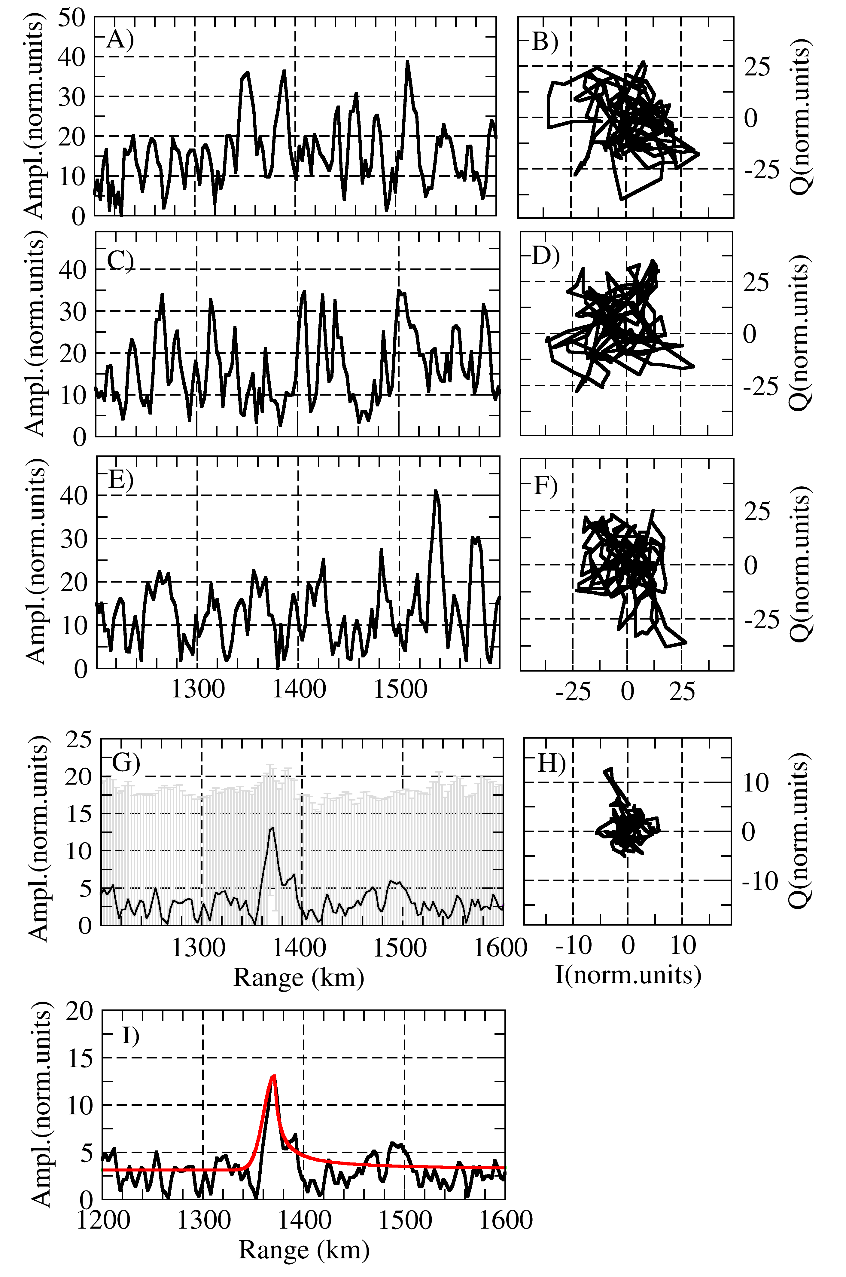
Figure 5: Noise signals - amplitude (A,C,E,G,I) and phase diagrams (B,D,F,H). A-F) 3 consequent realizations in the group G-H) Elementary response calculated over 30 sounding pulses (~300 msec). Grey color at G) corresponds to RMS during accumulation. The red line line at I) shows the approximation of the accumulated signal by the model (6).

It can be seen from the figures that elementary responses in the GS signals, in contrast to the IS signals and noise, have essentially asymmetric shape and longer back edge than the front one.

3.3 Parameters of elementary response shape

Let us check the regularity of the observed asymmetry over the experimental data. To do this we use the following unified model that can approximate elementary responses both in the GS signals and in the IS signals:

$$a(t,\{A,B,C,D\})=D+\left\{\begin{array}[]{l}Ae^{-\left(\frac{{}^{t-\tau_{0}}}{C}\right)^{2}};t<\tau_{0}\\ \frac{A}{1+(t-\tau_{0})/B};t>\tau_{0}\end{array}\right.$$ (6)

where $\tau_{0}$ is the radar delay to the maximal amplitude of the scattered signal; $A$ is the maximal amplitude of the accumulated signal; $B$ and $C$ are the parameters to be estimated, that characterize the duration of the left and right edges, respectively; $D$ is the noise level.

The choice of this model can be qualitatively justified by the shape of the asymptotic solution for the GS power, characterized by a sharp front edge, and by the smooth back edge Tinin (1983); Bliokh . (1988). The comb amplitude structure of the accumulated signal, as well as its phase structure has not been investigated in the paper.

Parameters $A,B,C,D$ are estimated by fitting the elementary response by the model (6). The model is linear over the $A,D$ and nonlinear over $B,C$. So $A,D$ can be calculated analytically. To speed up the search for $B$ and $C$ we use an integral approach: the integrals of the elementary response on the left and right of $\tau_{0}$ should be equal to the corresponding integrals of the model function:

$$\left\{\begin{array}[]{l}\int_{\tau_{0}}^{\infty}(a(t,\{A,B,C,D\})-D)dt=\int_{\tau_{0}}^{\infty}(U(t)-D)dt\\ \\ \int_{0}^{\tau_{0}}(a(t,\{A,B,C,D\})-D)dt=\int_{0}^{\tau_{0}}(U(t)-D)dt\end{array}\right.$$ (7)

The duration of left and right edges $T_{R},T_{L}$ of elementary response are calculated from the model parameters $B,C$. To determine them we search for the points at which the model function (6) value becomes equal to the given threshold level $\varepsilon_{L,R}$:

$$\left\{\begin{array}[]{l}a(t-T_{L},\{A,B,C,D\})=\varepsilon_{L}A+D\\ a(t+T_{R},\{A,B,C,D\})=\varepsilon_{R}A+D\end{array}\right.$$ (8)

When the model (6) is fitted into a real sounding signal of $300\mu s$ duration, each of the calculated edge durations $T_{L},T_{R}$ should be equal to $150\mu s$ (half of the sounding pulse duration). Thus we determine the values of these threshold levels: $\varepsilon_{L}=0.5,\varepsilon_{R}=0.2$. The obtained values of $T_{L},T_{R}$ are used to estimate duration of the elementary response edges directly in kilometers or microseconds. Fitting examples are shown in Fig.3I,4I,5I by red line.

By using the technique described above, we calculated the statistical distributions of the duration of the left and right edges of elementary responses in IS and GS signals over the experimental data set. The results are shown in Fig.6A-B. One can see that the characteristics of the elementary responses in different signal types are different: the elementary responses in GS signals (Fig.6A) are more asymmetric and have smoother right edge in comparison with the right edge of the elementary responses in IS signals (Fig.6B). At the same time, the elementary response in IS signal has relatively symmetrical edges. This does not contradict the previously described models for GSTinin (1983) and IS Grkovich  Berngardt (2011) signals, and validates the use of these models in the problem under consideration.

3.4 Elementary response lifetimes

Let us investigate the characteristic lifetimes of elementary responses. We estimate the lifetime by analysing the normalized cross-correlation coefficient between two different realizations, as a function of the delay between them. Following the approach described above the calculation of the correlation coefficient is made over a region of maximal signal-to-noise ratio near the delay $\tau_{0}$ (see Fig.2A). The duration of the region is determined by expected duration of the right and left edges $T_{R,0},T_{L,0}$. The correlation coefficient becomes:

$$R(i)=max_{n}\left\{R_{n,n+i}=\frac{\int_{\tau_{0}-T_{L,0}}^{\tau_{0}+T_{R,0}}u_{n}(\tau)u_{n+i}^{*}(\tau)d\tau}{\sqrt{\int_{\tau_{0}-T_{L,0}}^{\tau_{0}+T_{R,0}}|u_{n}(\tau)|^{2}d\tau\int_{\tau_{0}-T_{L,0}}^{\tau_{0}+T_{R,0}}|u_{n+i}(\tau)|^{2}d\tau}}\right\}$$ (9)

where $u_{n}^{*}$ is the complex conjugate value of the signal $u_{n}$ received in n-th realization.

As one can see in Fig.3,6A, the duration of ground scatter signal in a single realization (before its coherent accumulation) can reach up to 200-300 km. At the same time, the duration of the left edge for both kinds of signals usually does not exceed 60 km ($400\mu s$, see Fig.6A-B). Therefore, we choose the following values for the duration of the right and left edges used for calculation of correlation coefficient (9) $T_{R,0}=400\mu s$, $T_{L,0}=1600\mu s$.

For a detailed analysis of the elementary response lifetime we developed an algorithm, that works for arbitrary lags, both smaller and exceeding the duration of the whole sounding sequence (70 ms). The main property of the sounding sequences is related with the properties of Golomb rulers Berngardt, Voronov  Grkovich (2015): the combinational lags between different sounding pulses are always different and practically uniformly cover the region of lags within the duration of the sounding sequence. So for delays less than sounding sequence duration we calculate the correlation coefficient between elementary responses separated by delays (lags) corresponding to the combinational lags between the sounding pulses. This approach looks close to calculating autocorrelation function (ACF) by standard SuperDARN processing technique. To evaluate the correlation coefficient at large lags exceeding the duration of the sounding sequence we calculate it at lags corresponding to the delay between the first sounding pulse of each sounding sequence and the pulses of all subsequent sounding sequences. Then we average correlation coefficient at each obtained lag over the available pairs with identical lag between them. Analysis of the correlation coefficient at so large lags traditionally is not carried out at SuperDARN radars and at EKB radar. Most often this is associated with the complexity of total synchronization of all sounding sequences. The described algorithm allows us to obtain the correlation function of elementary responses at lags both less and greater than sounding sequence length.

Examples of the obtained correlation function for different kinds of scattered signals are shown in Fig.6C-H. It can be seen from the Fig.6C-E that the elementary responses in GS and IS signals differ significantly from the elementary responses in the noise - they have higher correlation coefficient at small lags. In Fig.6D,G it is shown that the correlation coefficient of elementary responses in IS signals increases at small lags, and this allows us to interpret the IS signal as a result of scattering by scatterers with a relatively short lifetime (hundreds of milliseconds). When the SNR decreases, the feature still persists, although it becomes less pronounced, and the maximum correlation coefficient at small lags decreases. This does not contradict with field-aligned irregularities lifetime estimated in other experiments Villain . (1996).

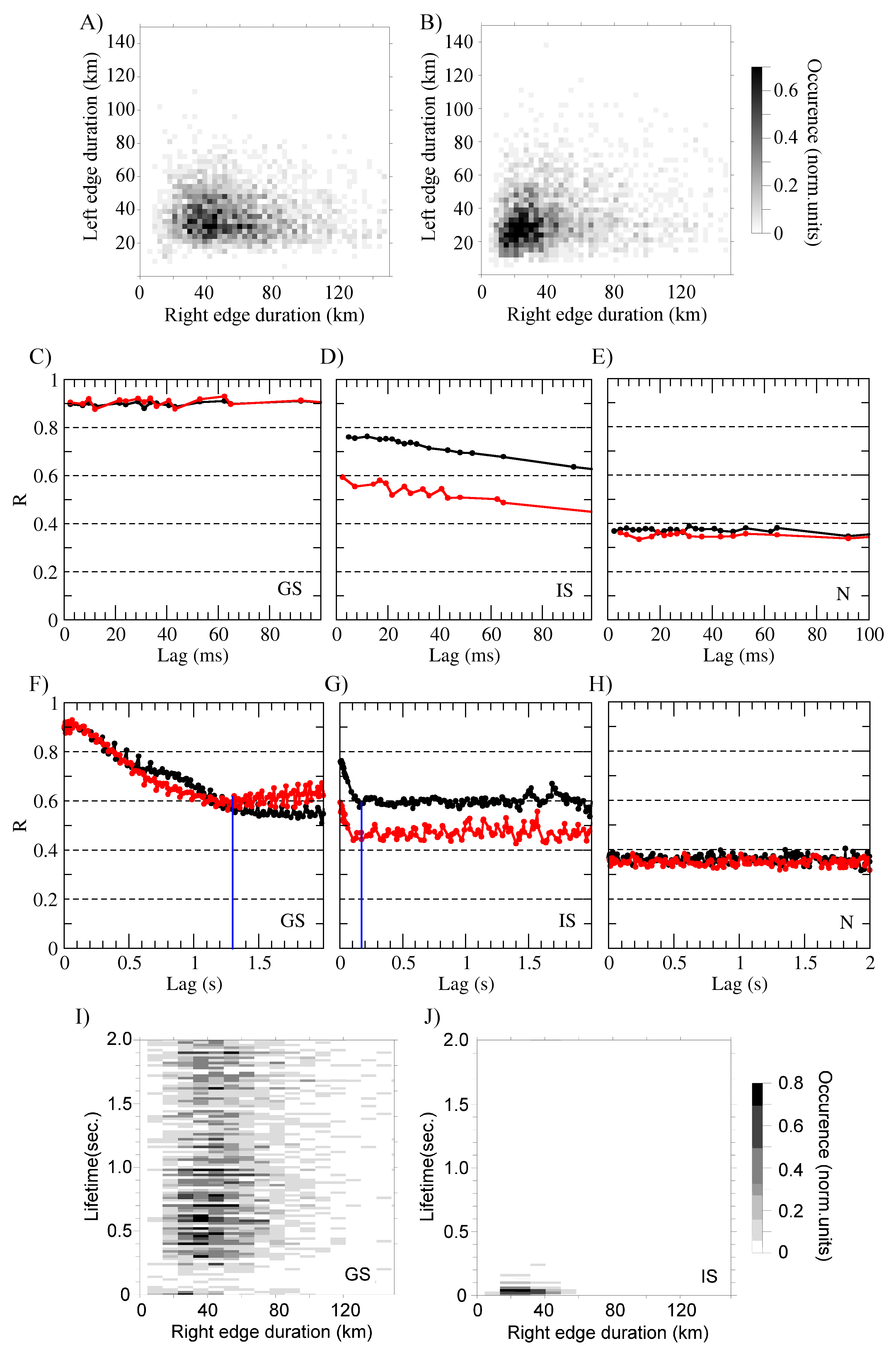
Figure 6: A-B) are the distributions of edges duration of the received signals: A) is the distribution for GS; B) is the distribution for IS. C-H) - correlation coefficient for different signal types. C-E) are is correlation coefficient at small lags comparable with sounding sequence duration for elementary response in GS (C), in IS (D), and in noise (E) signals; F-H) is correlation coefficient at large lags comparable with averaging interval in regular sounding mode, for elementary response in GS (F), in IS (G) and in noise (H) signals. Blue vertical line at (D-E) corresponds to elementary response lifetime. Black and red lines at A-F correspond to different experiments; I-J) - distributions of elementary responses over their lifetime (in seconds) and the right edge duration (in km.) for GS (I) and for IS (J) signals.

Fig.6C,F show that correlation coefficient of elementary responses in GS signals also decreases with a lag, but the characteristic rate is much lower and elementary response lifetime in GS is longer than in IS. From Fig.6C-D one can see, that in some cases it is difficult to differ GS from IS by lifetime using lags, provided by standard sounding sequences. This corresponds to small IS spectral widths case.

The analysis of correlation at extra large lags, compared with whole averaging interval for regular sounding, is shown in Fig.6F-H. It can be seen from Fig.6F-H that the average lifetime of elementary responses in GS signals ($>$1s) exceeds the lifetime of elementary responses in IS signals($<$250ms). This corresponds well with the physics of the signal formation. GS signal is a signal scattered by nearly stationary surface inhomogeneties. Its nonstationarity is mainly related with the existence of medium- and large-scale ionospheric irregularities. They affect the refraction of this signal and cause its decorrelation with time. The lifetime of individual small-scale irregularities (causing IS signals) is short. It can be estimated from the spectral width of the IS signals ($>4Hz$,$>40m/s$), and therefore rarely exceeds $250ms$. Thus, the measured elementary response lifetime does not contradict with known characteristics of IS signals.

In Fig.6F-G one can see that correlation coefficient falls with delay (’lag’) and reaches a certain stable (’noise’) level. So we define the elementary response lifetime as the delay at which the correlation coefficient becomes lower than certain threshold level $R_{th}$. This level is calculated over the lags larger than 2 sec:

$$\begin{array}[]{l}R_{th}=<R>+\Delta R\\ \\ <R>=\frac{1}{T_{2}-T_{1}}\int_{T_{1}=2sec}^{T_{2}>T_{1}}R(t)dt\\ \\ \Delta R=\sqrt{\frac{1}{T_{2}-T_{1}}\int_{T_{1}=2sec}^{T_{2}>T_{1}}(R(t)-<R>)^{2}dt}\end{array}$$ (10)

This approach allows us to automatically calculate the elementary response lifetime.

4 Identification of IS and GS signals

It was shown above that elementary response in GS and IS signals have different shape and different lifetime. This allows us to construct effective technique for identifying these signals by their amplitude-phase and correlation characteristics.

One of the standard approaches to signal identification is the method for testing statistical hypotheses Lehmann  Romano (2005). This method reduces the problem of separating signals to the problem of determining the detection boundary shape in the multidimensional space of signal characteristics. The signals inside the boundary are identified as IS signals, and the signals outside the boundary are identified as GS signals. There are several methods of making such a boundary shape, and they are based on minimizing the sum of the errors of the first and second kind (errors of incorrect acceptance and incorrect rejection of the hypothesis). We used the simplest Bayesian inference, under assumption of the equal probability of IS and GS signals.

To calculate boundary for identification algorithm, we used the distribution of elementary response characteristics in a three-dimensional parameter space (the duration of the right edge, the duration of the left edge, and the lifetime). In Fig.6I-J) it is shown that the distribution of elementary response parameters for IS signal lies within a bounded region in the parameter space. It is bounded by a certain surface around the coordinates center (small lifetimes, short right edges). The parameters of elementary responses in GS signal are outside the region (large lifetimes, long right edges). In the first approximation, there is no significant correlation between the duration of the right edge and the lifetime (Fig.6I-J), as well as between the left and right edges (Fig.6A-B). So we use an ellipsoid with the axes along the coordinate axes as separation boundary:

$$\frac{x^{2}}{a^{2}}+\frac{y^{2}}{b^{2}}+\frac{z^{2}}{c^{2}}=1$$ (11)

The coordinates x, y and z are the elementary response lifetime, the duration of the left edge and the duration of the right edge of the elementary response, respectively. The ellipsoid axis sizes - $a,b,c$ are to be determined. Elementary responses with parameters inside this boundary (11) correspond to IS signals, other correspond to GS signals.

To determine the parameters of the boundary, three-dimensional discrete distributions of elementary response parameters $P_{IS}(x,y,z)$ and $P_{GS}(x,y,z)$ were constructed from two experimental data sets (for GS and for IS). The step of the discretization of distributions over the lifetime was 2.5 ms, and over the left and right edges - 3 km. The search for the optimal values of the parameters $a,b,c$ was made numerically, by a direct search over the grid. The optimum condition was the Bayesian criterion minimizing the sum of errors of the first and second kind:

$$\Omega=\int_{r\left(\theta,\alpha\right)>\rho_{d}\left(\theta,\alpha\right)}P_{IS}(x,y,z)dxdydz+\int_{r\left(\theta,\alpha\right)<\rho_{d}\left(\theta,\alpha\right)}P_{GS}(x,y,z)dxdydz=min$$ (12)

Using polar coordinates $\left(r,\theta,\alpha\right)$ allows us to reduce the separation problem to checking the conditions $r\left(\theta,\alpha\right)>\rho_{d}\left(\theta,\alpha\right)$ and $r\left(\theta,\alpha\right)<\rho_{d}\left(\theta,\alpha\right)$, where $\rho_{d}\left(\theta,\alpha\right)$ is the equation of the ellipsoid surface in polar coordinates. Integration in the Cartesian coordinate system is made over the region outside the surface of the ellipsoid in the first term, and over the region inside this ellipsoid - in the second term. Search for optimum (12) over the data set with more than 13 thousand realizations gives the following separation boundary (11) parameters: a = 285 ms, b = 120 km, c = 429 km.

We use about 19 thousand realizations (13 thousand from training data set and 6 thousand from testing data set) to verify the technique. The results are shown in Fig.7. As our analysis has shown, the accuracy of GS identification is 95.1%. Accuracy of IS identification is 88.6%. The total identification error is 16.3%.

Figure 7: The results of identifying signal type by the new identification algorithm. At (A,C) blue dots mark the signals, identified as GS, red dots correspond to identification as IS signals. A) - results of processing GS signals; B) - peak SNR of GS signals; C) - results of processing IS signals; D) is the peak SNR of IS signals.

Fig.7 shows an examples of identification of the signal type for GS (Fig.7A) and IS (Fig.7C) signals. As one can see in Fig.7A,C, in most cases the algorithm works correctly and it does not depend on the SNR (Fig.7B,D). This is an indirect sign of the validity of the developed model and the identification technique.

5 Non-local character of the algorithm

Most of the used signal GS/IS identification algorithms are local ones: the signal type is determined only by its local characteristics, measured at a given spatio-temporal point. In the case of simple algorithms, for example, FitACF,v.2.5 from Radar Software Toolkit (RST-3.5) (2018); Blanchard . (2009), the radius of non-locality is constant and corresponds to spatial resolution (15-45 km) and temporal resolution (2-6 seconds) of measurements. In more complex algorithms, like Ribeiro . (2011), it is not constant and depends on the characteristics of the scattered signal and the scattering region.

Our algorithm is a non-local one. The algorithm estimates the type of signal not at the selected range, but in the range area. The size of this area is determined by the amplitude-phase structure of elementary response. To investigate the non-locality of the algorithm, we made a numerical simulation. We modeled simultaneous presence of two signals of different types, at different distances and with different amplitudes. This allows us to study the dependence of algorithm detection errors in different situations. We carried out numerical modeling in three variants of the problem: to determine the parameters of signals that have equal amplitudes; to identify the signals in case IS is more powerful than GS; to identify the signals in case GS is more powerful than IS.

The simulation results are shown in Fig.8A-C. It can be seen that the algorithm begins to mix the characteristics of two signals when they are observed simultaneously in the analysis window (when the distance between them $<200km$, Fig.8 A). In this case, the identified type of signal is inherited from the more powerful signal (Fig.8B,C). In case of signals of equal power, IS signal identification dominates (Fig.8A). The change in the width of the detected areas in Fig.8A-C is related to the change in the SNR, which affects the amount of data processed.

Figure 8: The results of the identification in a simulated case of two overlapping signals of different type. A) The signals have equal power B) GS signal is more powerful than IS; C) IS signal is more powerful than GS.

6 Comparison with other classification techniques

We have compared the effectiveness of our IQ-method with the techniques developed earlier FitACF,v.2.5 from Radar Software Toolkit (RST-3.5) (2018); Blanchard . (2009); Ribeiro . (2011) in their standard configuration described in the corresponding papers and available programs. To compare these techniques, we manually selected from the available EKB radar data 80 observation periods of GS observations and 51 periods of IS observations. In each of the selected periods, the nature of the signal according to expert judgment was not in doubt. The data used for the comparison is shown in Supporting Materials, areas are marked with closed regions. Data with SNR$>2$ were processed by all the mentioned identification algorithms.

For the analysis, data obtained in the following 8 days of 2017 and 2018 was used: 21/10/2017, 09/12/2017, 25/12/2017, 09/03/2018, 15/03/2018, 26/04/2018, 27/04/2018, 05/05/2018. The total number of analyzed cases of scattering was about 15 thousand.

In the analysis, each case of scattering was analyzed by each of the four algorithms. Example of signal type identification is shown in Fig.9A-D. The distribution of the GS flags for different signal types is shown in Fig.9E-F (Fig.9E - IS signals only, Fig.9E - GS signals only). The distribution of the errors is not the same for different methods. From Fig.9E-F one can see that Ribeiro . (2011) looks the most effective for detecting IS and GS signals (over the data it can identify).

The proposed IQ-algorithm showed the smallest value of the total error (the average total error is $13.3\%$). The error of GS incorrectly defined as IS is $11.2\%$, and the erroneous definition of IS as GS is $2.1\%$. The FitACF,v.2.5 from Radar Software Toolkit (RST-3.5) (2018) algorithm showed a generally worse accuracy in both cases ($26.3\%$ and $6.6\%$, respectively). Using the Blanchard . (2009) algorithm produce errors of $13.1\%$ and $15.6\%$, respectively. The smallest total error ($25.6\%$) of the three traditional algorithms was produced by the Ribeiro . (2011) algorithm, but it did not process a large number of scattered signals ($23.4\%$ GS and $54.9\%$ IS, see Fig.9C) at all, which was not considered an error in our estimates.

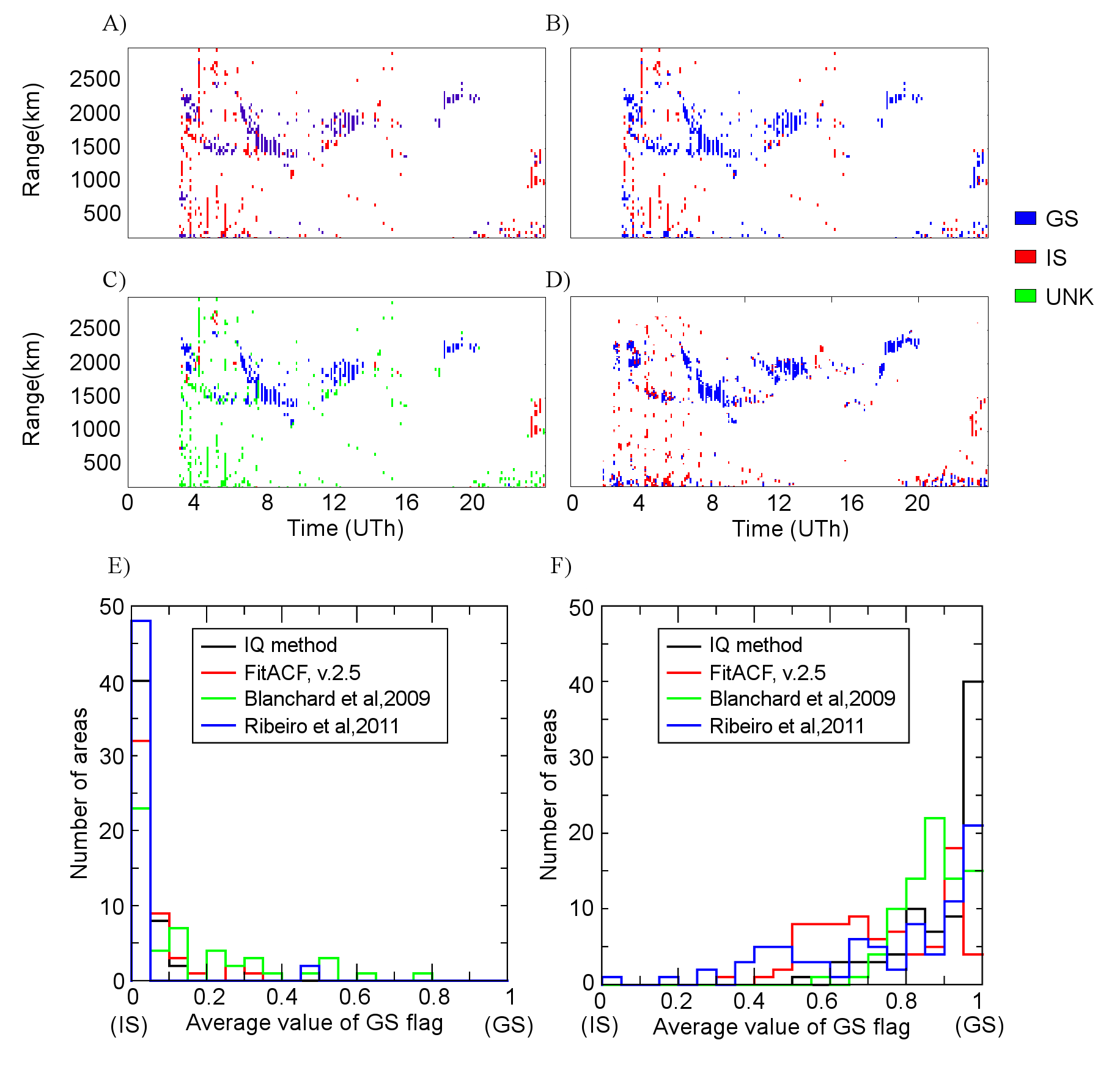
Figure 9: A) - Identification by FitACF,v.2.5 from Radar Software Toolkit (RST-3.5) (2018); B) - Identification by Blanchard . (2009); C) - Identification by Ribeiro . (2011); D) - Identification by our IQ method; Blue corresponds to GS, red to IS, green to unknown signals; E-F) The distribution of mean signal type over regions: E) - results of processing IS data; F) - results of processing GS data; Black, red, green and blue lines correspond to IQ method,FitACF,v.2.5 from Radar Software Toolkit (RST-3.5) (2018),Blanchard . (2009) and Ribeiro . (2011) methods correspondingly.

7 Conclusion

We made the analysis of the fine structure of decameter signals scattered by irregularities of the Earth’s surface and field-aligned ionospheric irregularities. The software of the EKB ISTP SB RAS radar was substantially modernized to carry out such an analysis with a high sampling frequency. Large number of experimental data with an increased sampling frequency has been obtained.

As a result of the experimental data analysis it is shown that signals scattered by both mechanisms have a specific phase structure and a nonzero lifetime. This allows us to interpret them as a superposition of elementary responses with a finite lifetime and specific amplitude-phase shape. An algorithm is constructed for estimating the shape of the elementary response. A unified empirical model of elementary response is developed, that allows us to describe both types of elementary response and to determine their characteristics - the lifetime, the duration of the right and left edges. Statistical features of elementary responses in GS and IS signals are estimated and presented. Differences in the properties of elementary responses in GS and IS signals are found: the different duration of the right front of the signal and different lifetimes.

Within the Bayesian inference approach and based on the analysis of the full waveform, a technique for the optimal identification of GS and IS signals was constructed. The technique (IQ method) works without using traditional SuperDARN algorithm for estimating scattered signal parameters (FitACF) - spectral width and Doppler drift velocity. It is based on the analysis of IQ components of the signal only.

The weakness of the method is the need for a relatively high SNR ($>2$), at smaller SNR it is unstable and should not be used. Another weakness of the method is its non-local character. It can incorrectly identify the type of signals separated by a distance of less than 200 km, identifying the type of signal by a more powerful signal. In addition, within the spatial resolution (45 km), it may incorrectly identify the GS signal as IS signal at the boundary between lower ranges GS signal and higher ranges noise.

The effectiveness of the method is estimated based on EKB radar data at SNR$>2$. It is shown that using this technique at EKB radar at SNR$>2$ produces less total error, than traditional algorithms FitACF,v.2.5 from Radar Software Toolkit (RST-3.5) (2018); Blanchard . (2009); Ribeiro . (2011). The total error (defined as the total ratio of incorrectly defined points in all areas to their total number) produced by our IQ-algorithm over the selected data was $13.3\%$. FitACF,v.2.5 from Radar Software Toolkit (RST-3.5) (2018) algorithm produces total error of $32.9\%$, Blanchard . (2009) method produces total error about $28.7\%$, Ribeiro . (2011) algorithm produces total error about $25.6\%$ (over the data, marked definitely as GS or IS).

So over test dataset of EKB radar data with SNR$>2$ our IQ algorithm provides noticeably higher accuracy in determining the type of signal than other methods. To identify signal types at low SNR ($<2$) or at 45 km boundary with noise, one can use the traditional local methods FitACF,v.2.5 from Radar Software Toolkit (RST-3.5) (2018); Blanchard . (2009) instead of this technique.

The work was supported by the RFBR grant # 16-05-01006a. In the paper EKB ISTP SB RAS radar data were used, the radar functioning is supported by the FSR program II.12. The data of EKB radar is a property of ISTP SB RAS, contact Oleg Berngardt (berng@iszf.irk.ru).

References

- Andre \BOthers. (\APACyear1999) \APACinsertmetastarAndre_1999{APACrefauthors}Andre, D., Pinnock, M.\BCBL \BBA Rodger, A. \APACrefYearMonthDay1999. \BBOQ\APACrefatitleOn the SuperDARN autocorrelation function observed in the ionospheric cusp On the SuperDARN autocorrelation function observed in the ionospheric cusp.\BBCQ \APACjournalVolNumPagesGeophys. Res. Lett.26223353–3356. {APACrefDOI} \doi10.1029/1999gl003658 \PrintBackRefs\CurrentBib
- Baker \BOthers. (\APACyear1988) \APACinsertmetastarBaker_1988{APACrefauthors}Baker, K., Greenwald, R., Villian, J.\BCBL \BBA Wing, S. \APACrefYearMonthDay1988. \APACrefbtitleSpectral Characteristics of High Frequency (HF) Backscatter for High Latitude Ionospheric Irregularities: Preliminary Analysis of Statistical Properties Spectral Characteristics of High Frequency (HF) Backscatter for High Latitude Ionospheric Irregularities: Preliminary Analysis of Statistical Properties \APACbVolEdTR\BTR \BNUM ADA202998. \APACaddressInstitutionJohns Hopkins Univ Laurel Md Applied Physics Lab. {APACrefURL} http://www.dtic.mil/cgi-bin/GetTRDoc?Location=U2&doc=GetTRDoc.pdf&AD=ADA202998 \PrintBackRefs\CurrentBib
- Barthes \BOthers. (\APACyear1998) \APACinsertmetastarBarthes_1998{APACrefauthors}Barthes, L., Andre, D., Cerisier, J\BPBIC.\BCBL \BBA Villain, J\BHBIP. \APACrefYearMonthDay1998. \BBOQ\APACrefatitleSeparation of multiple echoes using a high-resolution spectral analysis for SuperDARN HF radars Separation of multiple echoes using a high-resolution spectral analysis for SuperDARN HF radars.\BBCQ \APACjournalVolNumPagesRadio Sci.3341005–1017. {APACrefDOI} \doi10.1029/98rs00714 \PrintBackRefs\CurrentBib
- Berngardt \BOthers. (\APACyear2016) \APACinsertmetastarBerngardt_2016{APACrefauthors}Berngardt, O., Kutelev, K.\BCBL \BBA Potekhin, A. \APACrefYearMonthDay2016. \BBOQ\APACrefatitleSuperDARN scalar radar equations SuperDARN scalar radar equations.\BBCQ \APACjournalVolNumPagesRadio Science51101703 – 1724. {APACrefDOI} \doi10.1002/2016rs006081 \PrintBackRefs\CurrentBib
- Berngardt \BOthers. (\APACyear2018) \APACinsertmetastarBerngardt_2018{APACrefauthors}Berngardt, O., Ruohoniemi, J., Nishitani, N., Shepherd, S., Bristow, W.\BCBL \BBA Miller, E. \APACrefYearMonthDay2018. \BBOQ\APACrefatitleAttenuation of decameter wavelength sky noise during x-ray solar flares in 2013–2017 based on the observations of midlatitude HF radars Attenuation of decameter wavelength sky noise during x-ray solar flares in 2013–2017 based on the observations of midlatitude HF radars.\BBCQ \APACjournalVolNumPagesJournal of Atmospheric and Solar-Terrestrial Physics1731 - 13. {APACrefDOI} \doihttps://doi.org/10.1016/j.jastp.2018.03.022 \PrintBackRefs\CurrentBib
- Berngardt, Voronov\BCBL \BBA Grkovich (\APACyear2015) \APACinsertmetastarBerngardt_2015c{APACrefauthors}Berngardt, O., Voronov, A.\BCBL \BBA Grkovich, K. \APACrefYearMonthDay2015. \BBOQ\APACrefatitleOptimal signals of Golomb ruler class for spectral measurements at EKB SuperDARN radar: Theory and experiment Optimal signals of Golomb ruler class for spectral measurements at EKB SuperDARN radar: Theory and experiment.\BBCQ \APACjournalVolNumPagesRadio Science506486–500. {APACrefDOI} \doi10.1002/2014RS005589 \PrintBackRefs\CurrentBib
- Berngardt, Zolotukhina\BCBL \BBA Oinats (\APACyear2015) \APACinsertmetastarBerngardt_EPS{APACrefauthors}Berngardt, O., Zolotukhina, N.\BCBL \BBA Oinats, A. \APACrefYearMonthDay2015. \BBOQ\APACrefatitleObservations of field-aligned ionospheric irregularities during quiet and disturbed conditions with EKB radar: First results Observations of field-aligned ionospheric irregularities during quiet and disturbed conditions with EKB radar: First results.\BBCQ \APACjournalVolNumPagesEarth, Planets and Space67143. {APACrefDOI} \doi10.1186/s40623-015-0302-3 \PrintBackRefs\CurrentBib
- Blanchard \BOthers. (\APACyear2009) \APACinsertmetastarBlanchard_2009{APACrefauthors}Blanchard, G., Sundeen, S.\BCBL \BBA Baker, K. \APACrefYearMonthDay2009. \BBOQ\APACrefatitleProbabilistic identification of high-frequency radar backscatter from the ground and ionosphere based on spectral characteristics Probabilistic identification of high-frequency radar backscatter from the ground and ionosphere based on spectral characteristics.\BBCQ \APACjournalVolNumPagesRadio Science445RS5012. {APACrefDOI} \doi10.1029/2009rs004141 \PrintBackRefs\CurrentBib
- Bliokh \BOthers. (\APACyear1988) \APACinsertmetastarBliokh_1987{APACrefauthors}Bliokh, P., Galushko, V., Minakov, A.\BCBL \BBA Yampolski, Y. \APACrefYearMonthDay1988. \BBOQ\APACrefatitleField interference structure fluctuations near the boundary of the skip zone Field interference structure fluctuations near the boundary of the skip zone.\BBCQ \APACjournalVolNumPagesRadiophysics and Quantum Electronics316480–487. {APACrefDOI} \doi10.1007/bf01044650 \PrintBackRefs\CurrentBib
- Budden (\APACyear1985) \APACinsertmetastarBudden_1985{APACrefauthors}Budden, K. \APACrefYear1985. \APACrefbtitleThe Propagation of Radio Waves: The Theory of Radio Waves of Low Power in the Ionosphere and Magnetosphere The Propagation of Radio Waves: The Theory of Radio Waves of Low Power in the Ionosphere and Magnetosphere. \APACaddressPublisherCambridge University Press. {APACrefDOI} \doi10.1017/CBO9780511564321 \PrintBackRefs\CurrentBib
- Chisham \BOthers. (\APACyear2007) \APACinsertmetastarChisham_2007{APACrefauthors}Chisham, G., Lester, M., Milan, S., Freeman, M., Bristow, W., McWilliams, K.\BDBLWalker, A. \APACrefYearMonthDay2007. \BBOQ\APACrefatitleA decade of the Super Dual Auroral Radar Network (SuperDARN): scientific achievements, new techniques and future directions A decade of the Super Dual Auroral Radar Network (SuperDARN): scientific achievements, new techniques and future directions.\BBCQ \APACjournalVolNumPagesSurv Geophys28133-109. {APACrefDOI} \doi10.1007/s10712-007-9017-8 \PrintBackRefs\CurrentBib
- Farley (\APACyear1969) \APACinsertmetastarFarley_1969{APACrefauthors}Farley, D. \APACrefYearMonthDay1969. \BBOQ\APACrefatitleIncoherent Scatter Correlation Function Measurements Incoherent Scatter Correlation Function Measurements.\BBCQ \APACjournalVolNumPagesRadio Science410935–953. {APACrefDOI} \doi10.1029/rs004i010p00935 \PrintBackRefs\CurrentBib
- Farley (\APACyear1972) \APACinsertmetastarFarley_1972{APACrefauthors}Farley, D. \APACrefYearMonthDay1972. \BBOQ\APACrefatitleMultiple-Pulse Incoherent-Scatter Correlation Function Measurements Multiple-Pulse Incoherent-Scatter Correlation Function Measurements.\BBCQ \APACjournalVolNumPagesRadio Sci.76661–666. {APACrefDOI} \doi10.1029/rs007i006p00661 \PrintBackRefs\CurrentBib
- \APACcitebtitleFitACF,v.2.5 from Radar Software Toolkit (RST-3.5) (\APACyear2018) \APACinsertmetastarFitACF_25\APACrefbtitleFitACF,v.2.5 from Radar Software Toolkit (RST-3.5). FitACF,v.2.5 from Radar Software Toolkit (RST-3.5). \APACrefYearMonthDay2018. \APAChowpublishedhttps://github.com/SuperDARN/rst. \APACaddressPublisherGitHub. \PrintBackRefs\CurrentBib
- Greenwald \BOthers. (\APACyear1995) \APACinsertmetastarGreenwald_1995{APACrefauthors}Greenwald, R., Baker, K., Dudeney, J., Pinnock, M., Jones, T., Thomas, E.\BDBLYamagishi, H. \APACrefYearMonthDay1995. \BBOQ\APACrefatitleDarn/Superdarn: A Global View of the Dynamics of High-Lattitude Convection Darn/Superdarn: A Global View of the Dynamics of High-Lattitude Convection.\BBCQ \APACjournalVolNumPagesSpace Science Reviews71761–796. {APACrefDOI} \doi10.1007/BF00751350 \PrintBackRefs\CurrentBib
- Grkovich \BBA Berngardt (\APACyear2011) \APACinsertmetastarGrkovich_2011{APACrefauthors}Grkovich, K.\BCBT \BBA Berngardt, O. \APACrefYearMonthDay2011. \BBOQ\APACrefatitleThe Technique Of Coherent Echo Processing In The Approximation Of A Small Number Of Point Scatterers The Technique Of Coherent Echo Processing In The Approximation Of A Small Number Of Point Scatterers.\BBCQ \APACjournalVolNumPagesRadiophysics and Quantum Electronics547452-462. {APACrefDOI} \doi10.1007/s11141-011-9305-5 \PrintBackRefs\CurrentBib
- Grocott \BOthers. (\APACyear2013) \APACinsertmetastarGrocott_2013{APACrefauthors}Grocott, A., Hosokawa, K., Ishida, T., Lester, M., Milan, S., Freeman, M\BPBIP.\BDBLYukimatu, A. \APACrefYearMonthDay2013. \BBOQ\APACrefatitleCharacteristics of medium-scale traveling ionospheric disturbances observed near the Antarctic Peninsula by HF radar Characteristics of medium-scale traveling ionospheric disturbances observed near the Antarctic Peninsula by HF radar.\BBCQ \APACjournalVolNumPagesJournal of Geophysical Research: Space Physics11895830–5841. {APACrefDOI} \doi10.1002/jgra.50515 \PrintBackRefs\CurrentBib
- Hanuise \BOthers. (\APACyear1993) \APACinsertmetastarHanuise_1993{APACrefauthors}Hanuise, C., Villain, J\BHBIP., Grésillon, D., Cabrit, B., Greenwald, R.\BCBL \BBA Baker, K. \APACrefYearMonthDay1993. \BBOQ\APACrefatitleInterpretation of HF radar ionospheric doppler spectra by collective wave scattering-theory Interpretation of HF radar ionospheric doppler spectra by collective wave scattering-theory.\BBCQ \APACjournalVolNumPagesAnnales Geophysicae-Atmospheres Hydrospheres And Space Sciences11129-39. \PrintBackRefs\CurrentBib
- Hayashi \BOthers. (\APACyear2010) \APACinsertmetastarHayashi_2010{APACrefauthors}Hayashi, H., Nishitani, N., Ogawa, T., Otsuka, Y., Tsugawa, T., Hosokawa, K.\BCBL \BBA Saito, A. \APACrefYearMonthDay2010. \BBOQ\APACrefatitleLarge-scale traveling ionospheric disturbance observed by superDARN Hokkaido HF radar and GPS networks on 15 December 2006 Large-scale traveling ionospheric disturbance observed by superDARN Hokkaido HF radar and GPS networks on 15 December 2006.\BBCQ \APACjournalVolNumPagesJ. Geophys. Res.115A6A06309. {APACrefDOI} \doi10.1029/2009ja014297 \PrintBackRefs\CurrentBib
- Ishimaru (\APACyear1999) \APACinsertmetastarIshimaru_1999{APACrefauthors}Ishimaru, A. \APACrefYear1999. \APACrefbtitleWave Propagation and Scattering in Random Media Wave Propagation and Scattering in Random Media. \APACaddressPublisherWiley-IEEE Press. \PrintBackRefs\CurrentBib
- Lehmann \BBA Romano (\APACyear2005) \APACinsertmetastarLehman_2005{APACrefauthors}Lehmann, E.\BCBT \BBA Romano, J. \APACrefYear2005. \APACrefbtitleTesting Statistical Hypotheses Testing Statistical Hypotheses. \APACaddressPublisherSpringer New York. {APACrefDOI} \doi10.1007/0-387-27605-x \PrintBackRefs\CurrentBib
- Lester \BOthers. (\APACyear2004) \APACinsertmetastarLester_2004{APACrefauthors}Lester, M., Chapman, P., Cowley, S., Crooks, S., Davies, J., Hamadyk, P.\BDBLBarnes, R. \APACrefYearMonthDay2004. \BBOQ\APACrefatitleStereo CUTLASS–a new capability for the SuperDARN HF radars Stereo CUTLASS–a new capability for the SuperDARN HF radars.\BBCQ \APACjournalVolNumPagesAnnales Geophysicae222459-473. {APACrefDOI} \doi10.5194/angeo-22-459-2004 \PrintBackRefs\CurrentBib
- Liu \BOthers. (\APACyear2012) \APACinsertmetastarLiu_2012{APACrefauthors}Liu, E., Hu, H., Liu, R., Wu, Z.\BCBL \BBA Lester, M. \APACrefYearMonthDay2012. \BBOQ\APACrefatitleAn adjusted location model for SuperDARN backscatter echoes An adjusted location model for SuperDARN backscatter echoes.\BBCQ \APACjournalVolNumPagesAnnales Geophysicae30121769–1779. {APACrefDOI} \doi10.5194/angeo-30-1769-2012 \PrintBackRefs\CurrentBib
- Milan \BOthers. (\APACyear1997) \APACinsertmetastarMilan_1997{APACrefauthors}Milan, S., Yeoman, T., Lester, M., Thomas, E.\BCBL \BBA Jones, T. \APACrefYearMonthDay1997. \BBOQ\APACrefatitleInitial backscatter occurrence statistics from the CUTLASS HF radars Initial backscatter occurrence statistics from the CUTLASS HF radars.\BBCQ \APACjournalVolNumPagesAnn. Geophys.15703-718. {APACrefDOI} \doi10.1007/s00585-997-0703-0 \PrintBackRefs\CurrentBib
- Moorcroft (\APACyear1987) \APACinsertmetastarMoorcroft_1987{APACrefauthors}Moorcroft, D. \APACrefYearMonthDay1987. \BBOQ\APACrefatitleEstimates of absolute scattering coefficients of radar aurora Estimates of absolute scattering coefficients of radar aurora.\BBCQ \APACjournalVolNumPagesJournal of Geophysical Research: Space Physics92A88723–8732. {APACrefDOI} \doi10.1029/ja092ia08p08723 \PrintBackRefs\CurrentBib
- Moorcroft (\APACyear2004) \APACinsertmetastarMoorcroft_2004{APACrefauthors}Moorcroft, D. \APACrefYearMonthDay2004. \BBOQ\APACrefatitleThe shape of auroral backscatter spectra The shape of auroral backscatter spectra.\BBCQ \APACjournalVolNumPagesGeophysical Research Letters319L09802. {APACrefDOI} \doi10.1029/2003gl019340 \PrintBackRefs\CurrentBib
- Parris \BOthers. (\APACyear2008) \APACinsertmetastarParris_2008{APACrefauthors}Parris, R\BPBIT., Bristow, W., Shuxiang, S.\BCBL \BBA Spaleta, J. \APACrefYearMonthDay2008. \BBOQ\APACrefatitleFirst Results of Imaging, Super Stereo, and Other Upgrades on the Kodiak Radar First Results of Imaging, Super Stereo, and Other Upgrades on the Kodiak Radar.\BBCQ \BIn \APACrefbtitleSuperDARN Wokrshop, Newcastle, Australia. June 2008. SuperDARN Wokrshop, Newcastle, Australia. June 2008. (\BPG n/a). \PrintBackRefs\CurrentBib
- Ponomarenko \BBA Waters (\APACyear2006) \APACinsertmetastarPonomarenko_2006{APACrefauthors}Ponomarenko, P.\BCBT \BBA Waters, C\BPBIL. \APACrefYearMonthDay2006. \BBOQ\APACrefatitleSpectral width of SuperDARN echoes: measurement, use and physical interpretation Spectral width of SuperDARN echoes: measurement, use and physical interpretation.\BBCQ \APACjournalVolNumPagesAnnales Geophysicae241115–128. {APACrefDOI} \doi10.5194/angeo-24-115-2006 \PrintBackRefs\CurrentBib
- Reimer \BOthers. (\APACyear2016) \APACinsertmetastarReimer_2016{APACrefauthors}Reimer, A., Hussey, G.\BCBL \BBA Dueck, S. \APACrefYearMonthDay2016. \BBOQ\APACrefatitleOn the statistics of SuperDARN autocorrelation function estimates On the statistics of SuperDARN autocorrelation function estimates.\BBCQ \APACjournalVolNumPagesRadio Science516690–703. {APACrefDOI} \doi10.1002/2016rs005975 \PrintBackRefs\CurrentBib
- Ribeiro (\APACyear2018) \APACinsertmetastarRibeiro_Cluster{APACrefauthors}Ribeiro, A. \APACrefYearMonthDay2018. \APACrefbtitleClassification of SuperDARN backscatter using machine learning algorithms. Classification of SuperDARN backscatter using machine learning algorithms. \APAChowpublishedhttps://github.com/vtsuperdarn/clustering_superdarn_data. \APACaddressPublisherGitHub. \PrintBackRefs\CurrentBib
- Ribeiro, Ponomarenko\BCBL \BOthers. (\APACyear2013) \APACinsertmetastarRibeiro_2013b{APACrefauthors}Ribeiro, A., Ponomarenko, P., Ruohoniemi, J., Baker, J., Clausen, N., Greenwald, R.\BCBL \BBA de Larquier, S. \APACrefYearMonthDay2013. \BBOQ\APACrefatitleA realistic radar data simulator for the Super Dual Auroral Radar Network A realistic radar data simulator for the Super Dual Auroral Radar Network.\BBCQ \APACjournalVolNumPagesRadio Science483283–288. {APACrefDOI} \doi10.1002/rds.20032 \PrintBackRefs\CurrentBib
- Ribeiro \BOthers. (\APACyear2011) \APACinsertmetastarRibeiro_2011{APACrefauthors}Ribeiro, A., Ruohoniemi, J., Baker, J., Clausen, S., de Larquier, S.\BCBL \BBA Greenwald, R. \APACrefYearMonthDay2011. \BBOQ\APACrefatitleA new approach for identifying ionospheric backscatter in midlatitude SuperDARN HF radar observations A new approach for identifying ionospheric backscatter in midlatitude SuperDARN HF radar observations.\BBCQ \APACjournalVolNumPagesRadio Sci.46RS4011. {APACrefDOI} \doi10.1029/2011RS004676 \PrintBackRefs\CurrentBib
- Ribeiro, Ruohoniemi\BCBL \BOthers. (\APACyear2013) \APACinsertmetastarRibeiro_2013{APACrefauthors}Ribeiro, A., Ruohoniemi, J., Ponomarenko, P., Clausen, L., Baker, J., Greenwald, R.\BDBLde Larquier, S. \APACrefYearMonthDay2013. \BBOQ\APACrefatitleA comparison of SuperDARN ACF fitting methods A comparison of SuperDARN ACF fitting methods.\BBCQ \APACjournalVolNumPagesRadio Science483274–282. {APACrefDOI} \doi10.1002/rds.20031 \PrintBackRefs\CurrentBib
- Ruohoniemi \BBA Greenwald (\APACyear2005) \APACinsertmetastarRuohoniemi_2005{APACrefauthors}Ruohoniemi, J.\BCBT \BBA Greenwald, R. \APACrefYearMonthDay2005. \BBOQ\APACrefatitleDependencies of high-latitude plasma convection: Consideration of interplanetary magnetic field, seasonal, and universal time factors in statistical patterns Dependencies of high-latitude plasma convection: Consideration of interplanetary magnetic field, seasonal, and universal time factors in statistical patterns.\BBCQ \APACjournalVolNumPagesJournal of Geophysical Research: Space Physics110A9A09204. {APACrefDOI} \doi10.1029/2004ja010815 \PrintBackRefs\CurrentBib
- Ruohoniemi \BOthers. (\APACyear1993) \APACinsertmetastarRuohoniemi_1993{APACrefauthors}Ruohoniemi, J., Greenwald, R., Villain, J\BHBIP., Baker, K., Newell, P.\BCBL \BBA Meng, C\BHBII. \APACrefYearMonthDay1993. \BBOQ\APACrefatitleCoherent HF radar backscatter from small-scale irregularities in the dusk sector of the subauroral ionosphere Coherent HF radar backscatter from small-scale irregularities in the dusk sector of the subauroral ionosphere.\BBCQ \APACjournalVolNumPagesJournal of Geophysical Research: Space Physics93A1112871-12882. {APACrefDOI} \doi10.1029/JA093iA11p12871 \PrintBackRefs\CurrentBib
- Rytov \BOthers. (\APACyear1988) \APACinsertmetastarRytov_1988{APACrefauthors}Rytov, S., Kravtsov, Y.\BCBL \BBA Tatarskii, V. \APACrefYear1988. \APACrefbtitlePrinciples of statistical radiophysics 2. Correlation theory of random processes. Principles of statistical radiophysics 2. Correlation theory of random processes. \PrintBackRefs\CurrentBib
- Tinin (\APACyear1983) \APACinsertmetastarTinin_1983{APACrefauthors}Tinin, M\BPBIV. \APACrefYearMonthDay1983. \BBOQ\APACrefatitleWave propagation in a medium with large-scale random irregularities Wave propagation in a medium with large-scale random irregularities.\BBCQ \APACjournalVolNumPagesIzvestiya Vysshikh Uchebnykh Zavedenij. Radiofizika (in Russian)2636-43. \PrintBackRefs\CurrentBib
- Villain \BOthers. (\APACyear1996) \APACinsertmetastarVILLAIN_1996{APACrefauthors}Villain, J\BHBIP., André, R., Hanuise, C.\BCBL \BBA Grésillon, D. \APACrefYearMonthDay1996. \BBOQ\APACrefatitleObservation of the high latitude ionosphere by HF radars: interpretation in terms of collective wave scattering and characterization of turbulence Observation of the high latitude ionosphere by HF radars: interpretation in terms of collective wave scattering and characterization of turbulence.\BBCQ \APACjournalVolNumPagesJournal of Atmospheric and Terrestrial Physics588943 - 958. {APACrefDOI} \doi10.1016/0021-9169(95)00125-5 \PrintBackRefs\CurrentBib
- Yukimatu \BBA Tsutsumi (\APACyear2002) \APACinsertmetastarYukimatu_2002{APACrefauthors}Yukimatu, A.\BCBT \BBA Tsutsumi, M. \APACrefYearMonthDay2002. \BBOQ\APACrefatitleA new SuperDARN meteor wind measurement: Raw time series analysis method and its application to mesopause region dynamics A new SuperDARN meteor wind measurement: Raw time series analysis method and its application to mesopause region dynamics.\BBCQ \APACjournalVolNumPagesGeophys. Res. Lett.29201981. {APACrefDOI} \doi10.1029/2002gl015210 \PrintBackRefs\CurrentBib