Short title: Oscillatory Stationary Population Identity

Abstract.

A population is considered stationary if the growth rate is zero and the age structure is constant. It thus follows that a population is considered non-stationary if either its growth rate is non-zero and/or its age structure is non-constant. We propose three properties that are related to the stationary population identity (SPI) of population biology by connecting it with stationary populations and non-stationary populations which are approaching stationarity. One of these important properties is that SPI can be applied to partition a population into stationary and non-stationary components. These properties provide deeper insights into cohort formation in real-world populations and the length of the duration for which stationary and non-stationary conditions hold. The new concepts are based on the time gap between the occurrence of stationary and non-stationary populations within the SPI framework that we refer to as Oscillatory SPI and the Amplitude of SPI.

Full Title: On the three properties of stationary populations and knotting with non-stationary populations

(To appear in Bulletin of Mathematical Biology, Springer)

Arni S.R. Srinivasa Rao and James R. Carey

1. Stationary population identity: History and inspirations from biological experiments

Stationary Population Identity (SPI) is about equality of two quantities: one is obtained from the age-distribution of a stationary population and the other is obtained from the remaining years to live (or remaining time to live) of these individuals. This equality which is closely associated with the concept of the life table (a mathematical model to represent age-specific mortality in a population) can be expressed in several other ways. Let $X$ be the set of elements representing the proportions of populations at each age of a stationary population at time $t$ and let $Y$ be the set of elements representing the remaining number of years (or remaining time units) left to live at each age, then SPI holds imply,

(1.1) $$X=Y.$$

In a strict sense $X$ consists of distinct elements and $Y$ consists of distinct elements. Let us take an element in $X$, say $p$. Then, there exists an age in the stationary population at which the proportion of the population to the total population is $p$. If the equation (1.1) is true, then that guarantees that one of the elements of $Y$ is also $p$.

The equation (1.1) is true in population life tables which are stationary in nature.

Introduced to the demography literature by Brouard ([27, 32]) using French life tables and to the population biology literature by Muller, Carey and their colleagues ([1, 2, 31]) using survival patterns of captive cohorts of insects, stationary population identity (SPI) is expressed as $f_{1}(a)=f_{2}(a)$, where $f_{1}(a)$ the fraction of individuals who are captured at age “$a$” (out of total population) is equal to $f_{2}(a)$ the proportion of individuals who have a remaining time units left to die (see Figure 1). Although SPI is observed in populations that are stationary (replacement-level growth), the vast majority of populations for both humans and non-human species are both non-stationary and non-stable (changing growth rate and/or age structure). All the relevant definitions used in this paper are provided in Table 1.

Example 1.

Consider individuals between the ages of 70 to 90 years as a stationary subpopulation of the larger stationary population depicted in Figure 1. According to the Stationary Population Identity (SPI), if 14.8% of the population are in this 70 to 90 year old subpopulation, then there also exists another sub-population of the same number (and percentage) of individuals who have between 70 and 90 years remaining (diagonal shaded area from 0 to 30 years in Figure 1).

In this article, we prove several new theoretical aspects of stationary and non-stationary populations while understanding the implications of SPI. Three prominent of them are listed below:

(i) Populations consist of both stationary and non-stationary components (Theorem 2),

(ii) Stationary subpopulations of a total populations also possess stationary components (Theorem 3),

(iii) Population that is transiently stationary over a finite or an infinite interval can be joined with non-stationary populations (oscillatory property) (Theorems 6 and 7).

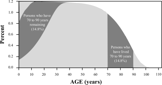
Figure 1. Illustration of the stationary population identity in which LL equals LR. Graphic is based on the U.S. 2006 female life table in which 14.8% of the life table population falls between 70 and 90 years of age (i.e., life-lived). This percentage is identical to the percentage of individuals in this same hypothetical stationary population who have from 70 to 90 years remaining (i.e., life-left).

Discovery of the SPI by Carey, originally referred to as Carey’s Equality ([29], [34]) but now referred to as SPI after the revelation that Brouard’s earlier papers also documented this identity (see [31]), was an outcome of a 10- year, U.S. National Institute on Aging-funded research program directed by biodemographer James R. Carey designed to study aging in the wild. This led to the identification of the relationship between population age structure and post-capture life spans of individuals through the use of a simple four-age class life table (Table 1 in [1]), the results of which were formulated mathematically for cases involving both stationary (i.e., SPI) and the non-stationary (with reference life tables) populations (see subsections on pp126-128 in [1]). Because of the importance to basic ecology and particularly to medical entomology where the older arthropod vectors (e.g., mosquitoes) have the highest likelihood of disease transmission, a great deal of effort has been invested in developing various technologies for estimating the age of individual insects including physiological [24], biochemical [25] and genetic [22, 23, 2, 19] methods.

The analytical evolution of this SPI continued with the publication of its proof, first as a demographic relationship between the life lived (LL) and life remaining (LR) [29] and then as a theorem and generalization [6]. A major mathematical breakthrough came in stationary population literature, when Rao and Carey [6] stated a new theorem using original ideas of stationary population principles (Carey - Rao Theorem on stationary population identity) through constructing arguments based on graphs and set-theoretic principles and based on two criteria that they stated on ‘LL’ and ‘LR’. The general concepts of the life table identify and its extension as an applied model (i.e., integration of reference life table information) have been used to estimate age structure and thus to gain insights into population aging in wild populations including effects of truncation studies [33], of fruit flies [20, 21], butterflies [28], and mosquitoes [30]. In light of the theoretical and analytical properties of SPI and its use as a foundation for developing models for estimating age structure in real-world insect populations, we believe that continuing to explore the mathematical properties of this identity has the potential to make new and original contributions to the demographic literature. Thus for the non-stationary and non-life table populations, the role of SPI needs thorough investigation.

$$\begin{array}[]{cc}\underline{\text{Item}}&\underline{\text{Definition}}\\ \\ \\ \text{SPI }&\text{\text{Two sets $X$ and }}Y\text{ such that}X=Y,\text{where }\\ \text{(Stationary Population Identity)}&\text{$X$ is the set of elements representing the }\\ &\text{ proportions of populationsat each age of a }\\ &\text{ stationary population at time $t$ and }Y\text{ is the set}\\ &\text{ of elements representing the remaining number of}\\ &\text{ years (or remaining time units) left to live at each age.}\\ \\ \text{}&\text{ SPI does not hold}\text{ When }X\neq Y\text{ in the above definition,}\\ &\text{we say that SPI does not hold.}\\ \\ \text{Knot}&\text{Joining of two simultaneous sub-intervals of time}\\ &\text{within [$t_{0}$,$t_{\omega}$), where in one sub-interval SPI holds, }\\ &\text{and other sub-interval SPI does not hold}\\ &\text{ }\\ &\text{}\\ \text{Predominantly }&\text{}\text{If a population during a time interval [$t_{0}$,$t_{\omega}$)}\\ \text{a Stationary Population}&\text{ satisfies the inequality}\\ \text{}&[t_{0},t_{1})\cup\stackrel{{\scriptstyle[}}{{M}},i=1]{\infty}{\bigcup}[\delta_{i},t_{i+1})>\stackrel{{\scriptstyle[}}{{N}},i=1]{\infty}{\bigcup}[t_{i},\delta_{i})\\ \text{}&\text{where SPI holds within }\\ &M=\left\{[t_{0},t_{1}),[\delta_{1},t_{2}),[\delta_{2},t_{3}),\cdots\right\}\\ &\text{and SPI does not holds within}\\ &N=\left\{[t_{1},\delta_{1}),[t_{2},\delta_{2}),\cdots\right\}\\ &\text{and intervals in }M\text{ and }N\text{ form partitions}\\ &\text{of }[t_{0},t_{\omega}).\\ \\ \text{Oscillatory SPI}&\text{SPI is oscillatory on the set $M$}\\ &\text{ with uniform amplitude if }\\ &\left\{t_{1}=\frac{t_{0}+\delta_{1}}{2},t_{2}=\frac{\delta_{1}+\delta_{2}}{2},t_{3}=\frac{\delta_{2}+\delta_{3}}{2},...\right\}\\ \\ \\ \end{array}$$

Table 1. Key Definitions Used in the Paper

2. Stationary and Non-Stationary populations

While exploring the deeper insights of SPI, we realized that this property can be helpful in knotting (read joining together) the concepts of stationary and non-stationary populations such that these two populations are formed on mutually-exclusive time intervals. A knot here we mean, joining of two simultaneous sub-intervals of time within $[t_{0},t_{\omega})$, where in one sub-interval SPI holds, and other sub-interval SPI does not hold. The main advantages of such a theoretical visualization of side-by-side occurrence of stationary and non- stationary populations are to keep our framework of SPI as flexible as possible such that realistic population dynamics are captured with respect to deviation from stationarity. Mathematically, these mutually exclusive concepts allow us to cut with knots the continuous interval on which we study simultaneous occurrences of these two types of populations. Our constructions in this article show that SPI property generates these knots on the continuous interval. Demarcation lines on an interval between stationary and non- stationary populations can then be visualized as dynamic. These demarcations (or boundary) lines led us to a novel concept within the SPI which we term Oscillatory SPI (O-SPI). In this case, the knots indicate the beginning of either stationary or non-stationary populations and allow us to introduce another term that we refer to on a continuous interval as the amplitude of the SPI.

For a predominantly stationary population (see Table 1 and the Definition 4) during an interval $[t_{0},t_{\omega})$, we can imagine that there exists a disjoint covering of intervals (a sub-collection of intervals, say $M$, in which SPI is true and other sub-collection of intervals, say, $N$, in which SPI is not true), such that,

$$\left(\bigcup_{C\in M}C\right)\cup\left(\bigcup_{C^{\prime}\in N}C^{\prime}\right)$$

equals $[t_{0},t_{\omega})$. The interval $[t_{0},t_{\omega})$ is visualized as a the union of two partitions, one which form SPI and other does not. See [4, 5] for concepts related to disjoint covering. The partition which form the identity is associated with stationary population and other one is associated non-stationary populations. If $``-"$ indicates the minus symbol, then, the SPI is true in $[t_{0},t_{\omega})-\bigcup_{C^{\prime}\in N}C^{\prime}$ and not true in $[t_{0},t_{\omega})-\bigcup_{C\in M}C.$ The value $[t_{0},t_{\omega})-\bigcup_{C^{\prime}\in N}C^{\prime}$ indicates the interval $[t_{0},t_{\omega})$ minus the intervals $\bigcup_{C^{\prime}\in N}C^{\prime},$i.e., if an element $x$ belongs $[t_{0},t_{\omega})-\bigcup_{C^{\prime}\in N}C^{\prime},$ then $x$ belongs to $[t_{0},t_{\omega})$ but $x$ does not to the union of intervals $\bigcup_{C^{\prime}\in N}C^{\prime}.$ Similarly, the meaning of $[t_{0},t_{\omega})-\bigcup_{C\in M}C$ can be interpreted. We develop an idea which we call uniform amplitude of SPI when equality such as (2.1) is true

(2.1) $$[t_{0},t_{\omega})-\bigcup_{\boldsymbol{C}\in M}C=[t_{0},t_{\omega})-\bigcup_{C^{\prime}\in N}C^{\prime},$$

and together $C=C^{\prime}$ holds for each simultaneous $C\in M$ and $C^{\prime}\in N.$ However, we develop these ideas on finite sets. Later we will see that the set $T$ in (2.2)

(2.2) $$T=\left\{[t_{0},t_{1}),[t_{1},\delta_{1}),[\delta_{1},t_{2}),\cdots[t_{k},\delta_{k-1}),[\delta_{k},t_{k+1}]\right\}$$

is a partition of $[t_{0},t_{k+1}]$, where $[t_{0},t_{k+1}]\subset[t_{0},t_{\omega}),$ such that each element of $[t_{0},t_{k+1}]$ lie in exactly in one interval in (2.2). We will also see in the Appendix that the set $\left\{I,J\right\}$ for the two intervals $I$, $J\subset[t_{0},t_{k+1}]$ as a partition of $[t_{0},t_{k+1}]$. Inasmuch as SPI connects these two properties in stationary populations, it follows that connecting them in non-stationary populations is a logical next step.

Let $\Omega$ be the size of the captive cohort such that $\Omega$ is an infinite subset or a very large finite subset of non-negative integers. Let $c_{i}$ be the age at capture and $d_{i}$ be the age at death of $i^{th}$ individual, where $d_{i}>c_{i}$ for each $i\in\Omega$. Here, $d_{i}-c_{i}$ is the follow-up length or post-capture LL by $i^{th}$ individual.

Theorem 2.

If a population is stationary then the SPI holds, but when $f_{1}(a)=f_{2}(a)$ does not hold for every age $``a"$ in a population then that population could be partitioned into stationary and non-stationary components.

Proof.

Idea: To prove the first part, we need to prove that if the population from which the captive cohort drawn is stationary then that follows SPI. For the second part, we first assume that$f_{1}(a)=f_{2}(a)$ is not true for every age $``a"$, and then we try to prove that the captive cohort $\Omega$ formed could be partitioned into stationary population and non-stationary population components.

We assume a very large number of individuals are captured at all possible ages (need not be integer valued) and no two individuals have same age at capture. We also assume that: (1) there will be a distinct value of duration of LR (i.e., remaining life to be lived after capture) corresponding to the each captured individual; and (2) one of the values of the remaining LR is identical to exactly one of the values of the age at capture. Let $\mu(\overline{c})$ and $\mu(\overline{d-c})$ be the average age at capture and average age of remaining length of post-capture life for the individuals in $J$, respectively, and $c_{1}\neq c_{2}\neq...\neq c_{k}\neq...$ and $d_{1}-c_{1}\neq d_{2}-c_{2}\neq...\neq d_{k}-c_{k}\neq...$., then we have

(2.3) $$\mu(\overline{c})=\frac{\Sigma_{i}c_{i}}{\left|\Omega\right|}\mbox{ and }\mu(\overline{d-c})=\frac{\Sigma_{i}(d_{i}-c_{i})}{\left|\Omega\right|}.$$

Suppose $S=\left\{s_{1},s_{2},...\right\}$, where $s_{i}=d_{i}-c_{i}$ for all $i\in\Omega.$ We can arrange elements of the set $S$ in a decreasing order. To do this, we set $s^{\prime}_{1}=\max\left\{s_{1},s_{2},...\right\}.$ Let $S_{1}=S-\left\{s^{\prime}_{1}\right\},$ where $S_{1}$ is the set of elements in $S$ after $s^{\prime}_{1}$ is removed. Let $s^{\prime}_{2}=\max\left\{S_{1}\right\}.$ We can continue to obtain maximum values, such that $S_{i+1}=S_{i}-\left\{s^{\prime}_{i+1}\right\},$ where $s^{\prime}_{i+1}=\max\left\{S_{i}\right\}$ for $i=1,2,\cdots$. Let $T=\left\{\left(1,s^{\prime}_{1}\right),\left(2,s^{\prime}_{2}\right),\cdots\right\}.$ The graph drawn through the co-ordinates of $T$ is a decreasing function. These kind of constructions for the information of LR after capture was originally used in [6]. When $s^{\prime}_{i}$ is equal to the corresponding individual’s age at capture for all $i\in J$ then the distribution of captured age is equal to the distribution of duration of the LR after capture. When $s^{\prime}_{j}$ is not equal to the corresponding individual’s age at capture for all $j\in\Omega_{1}$ for $\Omega_{1}\subset\Omega$, and $s^{\prime}_{i}$ is equal to the corresponding individual’s age at capture for all $i\in\Omega$ and $i\notin\Omega_{1}$. Then with a finite permutations of rearrangement of the elements in $\Omega_{1}$, we can match the set, $T^{\prime}=\left\{s^{\prime}_{1},s^{\prime}_{2},\cdots\right\}$ with $C,$ the set of decreasing values of captured ages, such that $T^{\prime}=C.$ With this construction explained, for an individual captured at the age “$a$” in $C$ (i.e., $a$ is an element in $C$) the value of the (element in $T^{\prime}$) is exactly “$a$” which is the remaining LR.

Suppose there are one or more than one individual of the same age at the time of capture. $\Omega$ is now sum of partitions of individuals, where each partition represents number of individuals who are captured at the same age. Let $c_{p}^{q}$ be the $q^{th}$ individual captured aged $p$ and $s_{p}^{q}$ be the remaining LR for the $q^{th}$ individual who was captured at age $p$ for $p>0$ and $q=1,2,\cdots,n_{p}$ $\left(n_{p}\in\mathbb{Z}^{+}\right).$ We assume that for each of the $s_{p}^{q}$ there is a corresponding value $c_{p}^{q}$ which could be within the same age $p$ or in other captured age. That is, if

$$C=\left\{c_{p}^{q}:\mbox{ }c_{p}^{q},p,\in\mathbb{R}^{+},q\in\mathbb{Z}^{+}\mbox{ and }1\leq q\leq n_{p}\right\}$$

and

$$S=\left\{s_{p}^{q}:\mbox{ }s_{p}^{q},p\in\mathbb{R}^{+},q\in\mathbb{Z}^{+}\mbox{ and }1\leq q\leq n_{p}\right\},$$

then for each $y\in S$ there is a corresponding element $x\in C.$ The following property is assured:

(2.4) $$\frac{\int_{0}^{\infty}\left(\sum_{q=0}^{n_{p}}c_{p}^{q}\right)dp}{\left|J\right|}=\frac{\int_{0}^{\infty}\left(\sum_{q=0}^{n_{p}}s_{p}^{q}\right)dp}{\left|J\right|}.$$

For more details on the type of logic and arguments provided above, see the Carey-Rao Theorem and proof [6], which introduced these set of arguments. Conversely, suppose for a finite population, let $f_{1}(a)=f_{2}(a)$ for the ages $a_{1},a_{2},\cdots,a_{k}$ (without any order) and $f_{1}(a)\neq f_{2}(a)$ for ages $a_{k+1},a_{k+2},\cdots,a_{n}$ (without any order) and no two individuals are of same age. This implies, there will be two vectors $V_{1}$ and $V_{2}$ based on the rule that SPI is true or not, which are given by,

$$V_{1}=\left[\begin{array}[]{c}f_{1}(a_{1})=f_{2}(a_{1})\\ f_{1}(a_{2})=f_{2}(a_{2})\\ \vdots\\ f_{1}(a_{k})=f_{2}(a_{k})\end{array}\right]\mbox{ and }\begin{array}[]{ccc}V_{2}&=&\left[\begin{array}[]{c}f_{1}(a_{k+1})\neq f_{2}(a_{k+1})\\ f_{1}(a_{k+2})\neq f_{2}(a_{k+2})\\ \vdots\\ f_{1}(a_{n})\neq f_{2}(a_{n})\end{array}\right].\end{array}$$

The sub-population corresponding to $V_{1}$ forms stationary population and the sub-population corresponding to $V_{2}$ forms non-stationary population. Due to $V_{2}$ the average value of the LL by $a_{1},a_{2},\cdots,a_{n}$ are not equal to their average remaining value, which will lead population to be non-stationary. ∎

Theorem 3.

Suppose SPI holds for a population, then a) SPI also holds for all stationary sub-populations of the original population and b) SPI need not hold for all non-stationary sub-populations of the original population.

Proof.

a) Let $P$ be a stationary population and let $P_{1},P_{2},...,P_{k}$ are disjoint stationary sub-populations and $Q_{1},Q_{2},...,Q_{l}$ are disjoint non-stationary sub-populations of $P$ such that

(2.5) $$\bigcup_{i=1}^{k}P_{i}\cup\bigcup_{j=1}^{l}Q_{j}=P.$$

If $P_{i}$ for each $i$ is a stationary population, then SPI holds within the each $P_{i}.$

b) Suppose we partition population into a disjoint collection of stationary and non-stationary sub-populations as in (a), then SPI need not hold in an arbitrarily chosen $Q_{j}$, because, for an arbitrarily chosen $Q_{j}$ the intrinsic growth rates could be very high and the population could be younger such that the proportion of population at age $a$ years not equal to the proportion of population who have $a$ years remaining. ∎

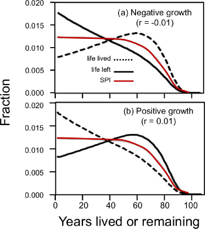
Figure 2. Relationship of the fraction of individuals who have lived x years relative to the fraction who have x years left to live for populations with either negative (a) or positive (b) growth rates. For reference the red curves shows the equivalency of LL and left for stationary populations (zero growth).

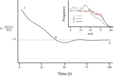
Figure 3. Trajectory of growth rate and age structure in a hypothetical population starting from a positive rate and converging to zero growth (stationarity). The initial age structure was based on the U.S. population in 2000, the fertility rates on a standard age-specific fertility schedule in humans scaled to replacement-level (=1.0) and survivorship on the female rates in 2006 [7]. N(t+1)/N(t) is the ratio of number in the population at time t+1 to the number at time and is denoted λ. Frequency in the inset refers to the age distribution of the population. Points labeled A, B, and C correspond to the starting growth rates, the point at which growth rate first reaches replacement level (i.e., transient stationarity), and the point at which growth rate is constant at zero (i.e., fixed stationarity), respectively. Replacement levels of growth required approximately 40 years from the start (i.e., A-to-B) and another 60 years to become fixed (i.e., B-to-C). Note the small oscillations around stationarity after B as the age structure converges to C.

3. Oscillatory stationary population identity and It’s Amplitude

Suppose that the population remains stationary for an infinitely long period of time, except in shorter time intervals in between due to perturbations. After small perturbations in the population due to vital events population deviates temporarily to a non-stationary state for a brief time-period before restoring stationary properties. When the population is stationary then we know that SPI holds (see for example [6]). SPI holds here we mean that it is true for all ages, i.e., the proportion of the population who are at age $a$ units is same as the proportion of the population who have $a$ units remaining for each age $a.$ Suppose the population remains stationary during the interval $\left[0,t\right]$ and let there be a vital event during the interval $(t,t+\delta)$ for a positive $\delta$ which is very very small. Then during $(t,t+\delta)$ SPI (in a strict sense) is not true and SPI remains not true until population remains strictly non-stationary (say until $\delta_{1}$ for $\delta_{1}>\delta$). As soon as stationarity is restored SPI will be true again until the next vital event. There will be finite or infinite cycles of stationary to non-stationary to stationary populations and hence SPI is true intermittently.

Definition 4.

We define a population as a predominantly a stationary population if

(3.1) $$[t_{0},t_{1})\cup\stackrel{{\scriptstyle[}}{{M}},i=1]{\infty}{\bigcup}[\delta_{i},t_{i+1})>\stackrel{{\scriptstyle[}}{{N}},i=1]{\infty}{\bigcup}[t_{i},\delta_{i}),$$

where SPI holds for the disjoint collection of intervals $M=\left\{[t_{0},t_{1}),[\delta_{1},t_{2}),[\delta_{2},t_{3}),\cdots\right\},$ and SPI does not hold for the disjoint collection of intervals $N=\left\{[t_{1},\delta_{1}),[t_{2},\delta_{2}),\cdots\right\}.$ The L.H.S. of (3.1) is the union over $i$ for the time intervals corresponding to the set $M$ and the R.H.S. of (3.1) is the union over $i$ values for the time intervals corresponding to the set $N.$ If

(3.2) $$[t_{0},t_{1})\cup\stackrel{{\scriptstyle[}}{{M}},i=1]{\infty}{\bigcup}[\delta_{i},t_{i+1})<\stackrel{{\scriptstyle[}}{{N}},i=1]{\infty}{\bigcup}[t_{i},\delta_{i}),$$

then we define a population as predominantly a non-stationary. A population is neither predominantly a stationary population nor predominantly a non-stationary if

(3.3) $$[t_{0},t_{1})\cup\stackrel{{\scriptstyle[}}{{M}},i=1]{\infty}{\bigcup}[\delta_{i},t_{i+1})=\stackrel{{\scriptstyle[}}{{N}},i=1]{\infty}{\bigcup}[t_{i},\delta_{i}).$$

We define oscillatory property of SPI as follows:

Definition 5.

We define a criteria that the SPI is oscillatory on $M$ with uniform amplitude whenever the following statement is true:

(3.4) $$\left\{t_{1}=\frac{t_{0}+\delta_{1}}{2},t_{2}=\frac{\delta_{1}+\delta_{2}}{2},t_{3}=\frac{\delta_{2}+\delta_{3}}{2},...\right\}.$$

Theorem 6.

For a predominantly stationary population defined in the Definition [4], SPI exists except for shorter intermittent intervals when population is non-stationary.

Proof.

Let the population be stationary during $[t_{0},t_{1})$ and a small perturbation (vital event(s)) takes place at $t_{1}$ such that the population deviates from stationary properties. Suppose there is a vital event(s) (at the time $\delta_{1}$ for some $\delta_{1}>t_{1}$), which balances deviated stationary population back to stationary mode. Suppose at time $t_{2}$ for $t_{2}>\delta_{1}$ the population again deviates from stationary mode due to vital event(s) and gets restored at time $\delta_{2}$ for $\delta_{2}>t_{2}$ such that the population remains non-stationary in the interval $[t_{2},\delta_{2}).$ Suppose this cycle of stationary population to non-stationary and back to stationary population continues to repeat at different time points $t$ and $\delta.$ SPI holds for the disjoint collection of intervals, $M$ and does not hold for the disjoint collection of intervals, $N.$ Because the population is predominantly stationary, the following inequality holds

(3.5) $$\frac{[t_{0},t_{1})\cup\stackrel{{\scriptstyle[}}{{M}},i=1]{\infty}{\bigcup}[\delta_{i},t_{i+1})}{\stackrel{{\scriptstyle[}}{{N}},i=1]{\infty}{\bigcup}[t_{i},\delta_{i})} > 1.$$

∎

Let us denote $\mathcal{S}_{0}=\frac{[t_{0},t_{1})\cup\stackrel{{\scriptstyle[}}{{M}},i=1]{\infty}{\bigcup}[\delta_{i},t_{i+1})}{\stackrel{{\scriptstyle[}}{{N}},i=1]{\infty}{\bigcup}[t_{i},\delta_{i})}.$

Whenever $\left[\Sigma_{i=1}^{\infty}(\delta_{i}-t_{i})\mbox{ for }\delta_{i},t_{i}\in N\right]$ $>\left[(t_{1}-t_{0})+\Sigma_{i=1}^{\infty}(t_{i+1}-\delta_{i})\mbox{ for }\delta_{i},t_{i}\in M\right]$, then $\mathcal{S}_{0}<1$.

We call this property of holding and not holding SPI over disjoint intervals constructed in the proof of the Theorem 6 as the O-SPI. We associate the idea of amplitude with the length of time when SPI holds. The amplitudes of SPI are defined here as the lengths of the intervals of the set $M.$

Theorem 7.

Given a finite time set-up of disjoint intervals of $M$ and $N$ up to $[\delta_{k},t_{k+1})\in M.$ If SPI is oscillatory on $M$ with uniform amplitude, then $\mathcal{S}_{0}=1$ but converse need not be true.

Proof.

When SPI is oscillatory on $M$ with uniform amplitude then the statement (3.4) is true. Hence we can see that

$\left[\Sigma_{i=1}^{\infty}(\delta_{i}-t_{i})\mbox{ for }\delta_{i},t_{i}\in N\right]$ $=\left[(t_{1}-t_{0})+\Sigma_{i=1}^{\infty}(t_{i+1}-\delta_{i})\mbox{ for }\delta_{i},t_{i}\in M\right]$, which implies $\mathcal{S}_{0}=1.$

Conversely, suppose $\mathcal{S}_{0}=1.$ Let us consider events up to time $t_{k+1}$ in the interval $[t_{0},\infty)$. Let $M_{t_{k+1}}$and $N_{t_{k+1}}$ be the sub-collection of intervals of $M$ and $N$, respectively and are given by,

$$M_{t_{k+1}} = \left\{[t_{0},t_{1}),[\delta_{1},t_{2}),[\delta_{2},t_{3}),\cdots,[\delta_{k},t_{k+1})\right\},$$

(3.6) $$N_{t_{k+1}} = \left\{[t_{1},\delta_{1}),[t_{2},\delta_{2}),\cdots,[t_{k},\delta_{k})\right\}.$$

For $k=1,$ we have,

$$M_{t_{2}} = \left\{[t_{0},t_{1}),[\delta_{1},t_{2})\right\},$$

(3.7) $$N_{t_{2}} = \left\{[t_{1},\delta_{1})\right\}.$$

Since $\mathcal{S}_{0}=1,$ from (3.7), we will have $t_{1}=\frac{t_{0}+2\delta_{1}-t_{2}}{2}.$ Since $t_{2}>\delta_{1}$, we have

(3.8) $$\frac{t_{0}+2\delta_{1}-t_{2}}{2}\neq\frac{t_{0}+\delta_{0}}{2}.$$

The inequality (3.8) indicates there is no uniform amplitude. ∎

Corollary 8.

For a predominantly non-stationary population SPI may hold even in small intermittent intervals.

4. Connection between main theorems, graphical results and applications

Several new properties and implications of SPI were proved in this article through various Theorems [Theorem 2, Theorem 3, Theorem 6, Theorem 7, Theorem 10 and Theorem 11] and Lemma 9. These theorems which take implications of SPI to different directions (for example, Theorem 2, Theorem 3, Theorem 6, Theorem 7) show newer avenues of the interface of SPI between stationary and non-stationary populations and O-SPI. Constructions of captive cohorts and logic of matching the duration of LL and LR developed in Carey - Rao Theorem on SPI [6] helped us to prove arguments in Theorem 2. This theorem implies that when the fraction of the population at age $a$ is not equal to the fraction of the population whose remaining years to live is $a$ for some age $a$, then the population could be either stationary or non-stationary. For a stationary population shown in Figure 1, these fractions are equal at all ages $a$ or at all age groups if group-wise fractions are considered. When these fractions are not equal for each age $a$ then the population is non-stationary. Therefore, Theorem 2 helped us investigate properties of the SPI that interface stationary and non-stationary populations.

An example of the relationship between the percentage of a population that have lived x years and the percentage of persons who have x years remaining in a stationary population is visualized in Figure 1 for a hypothetical population based on the 2006 U.S. female life table. This graphic shows that there are 14.8% of this stationary population that are aged 70 to 90 years old and, at the same time, there are 14.8% of the population who have from 70 to 90 years remaining. These percentages for remaining years are distributed among the younger individuals from newborn (x=0), most of whom have from 70 t 90 years remaining to a miniscule percentage of 40 year-olds who will live another 70 years (i.e., to super-centenarians, age 110). Theorem 3 is the first step towards specifying the behavior of SPI on partitions of stationary and non-stationary sub-populations of the total population. This implies, when partitioning of the total population is done into a collection of stationary sub-populations then the aforesaid fractions remain equal in each of the sub-population. Theorem 3 also implies that when a population is partitioned into sub-populations, these fractions need not be equal if stationary principles are not preserved (see Figure 2).

The relationship of the fraction of individuals in a population that have lived x years (i.e., the age distribution) relative to the fraction of individuals in the same population that have x years remaining is shown in Figure 2 for two hypothetical populations, one with a negative (r=-0.01) growth rate (Fig. 2a) and another with a positive (r=0.01) growth rate (Fig. 2b). Each is shown relative to the stationary (r=0.00) case. Several aspects of this figure merit comment. First, note the equivalency of the fraction of the population that have lived x years and the fraction that have x years to live as shown in the curves for the stationary population. In other words, the life-lived/life-left curves are superimposed. In contrast the trajectories for the life-lived and the life-left curves for populations with either negative or positive growth rates are separate as shown by the departure of the dashed and solid black lines in each graph. Note in the top graph for a population with the negative growth rate the fraction of the population that are young (e.g., 0 to 20 years is low relative the fraction that are old (e.g., 60 to 80 years). In other words, the age structure of decreasing populations is skewed to the older age classes. However, because population is older, the fraction of individuals with fewer number of years to live (e.g., <20) is higher relative to the fraction of persons who have many years left to live (e.g., >60 more years remaining). The exact opposite relationship of LL to LR is evident in a population a positive growth rate as shown in the bottom graph of Figure 2. That is, the skew towards the young in a growing population results in a skew toward the fraction of individual (i.e., the young) who have many years remaining.

Through Theorem 6, we have shown for a stationary population how SPI could hold in alternate time intervals. Within the construction of oscillatory properties, we have introduced amplitudes of SPI which provides the lengths of time intervals for which the SPI holds. We have introduced the idea of O-SPI which over the time will have practical applications in understanding population dynamics through switching of stationary and non-stationary populations (See both Figure 3 and next paragraph). The concept of transient stationarity is visualized in Figure 3 for a population converging from a positive growth rate to a fixed (replacement-level) stationary state. This figure shows the change in growth rate, $\lambda$, in the main graphic and the age structure of the population that corresponds to three different points (A, B, and C) along this growth trajectory. The age structure (inset) at $t=0$ corresponds to a growing population with a bi-modal distribution, one mode from birth to age 25 and the other from 25 to 50 years. This corresponds to point A in the main graphic (rapid growth rate). At around $t=40$ the population growth rate, λ, had decreased to zero (Point B). However, this was a transient condition because the age structure (shown in the inset) was not yet stable. This “transiency” in growth rate and age structure continued until both had converged to fixed stationarity, a state corresponding to point C in the main graphic showing changes in $\lambda$ and in the inset showing the age distribution. Connections between the properties of O-SPI and countries or populations with net reproduction rates (NRR) around the value one ($1.0$) can be investigated using the properties proved in this article. When the intrinsic growth rates are highly dynamic in the populations then achieving the net reproductive rates around the value one may not stay for a longer period, and the duration of the time for which the status of ´NRR = $1.0$´ in the population might be very short lived. Implications of ´NRR = $1.0$´ and properties of O-SPI across several populations can be studied to understand long-range population dynamics.

Since every human population has an underlying life table, every human population can form the basis of a model stationary population [8]. Therefore it follows that understanding the deeper properties of stationary populations as described here and elsewhere [9, 1, 6] will add important depth to population theory more generally. Second, understanding the oscillatory behavior of populations as they approach stationarity is important inasmuch as this behavior is tightly linked to the concept of population momentum—the continuation of growth after a population has achieved replacement-level fertility [10, 14, 3]. Momentum and population aging are essentially two aspects of the same phenomenon [11], and momentum is likely to be responsible for most of the future growth in the world’s population [12, 13]. Therefore, a deeper understanding of the underlying dynamics of population stationarity, momentum, and convergence and concepts concerned with the demographic transition will strengthen the foundations for the development of sound population policy including family planning, aging, and social security.

5. Discussion

The number of years different individuals have lived in a population, as well as the number of years these individuals have left, are universal properties of all populations. Whereas the first is a static characteristic of populations inasmuch as it specifies age structure, the second is a dynamic concept since it designates the future population’s actuarial properties. This second property is more complex than the first inasmuch as it describes distributions within a distribution i.e., the allocation of individual deaths within each of the 100+ age groups of the age distribution. Both of these population characteristics are important in both basic and applied demographic contexts. The first property is concerned with the relationship of different population age groups (e.g. dependency ratios; population aging) and the second is concerned with future deaths (e.g. how many deaths will occur in the next $1,2$, or $5$ years). Since the age structure of a population must logically be connected to its future death distribution, the implicit qualitative relationship between life-years lived and life- years is both obvious and intuitive. However, the explicit quantitative relationship between life-lived and left was neither obvious nor intuitive prior to the discovery of the SPI. Because of the importance of linking the actuarial properties of populations with their age structure as SPI does, it follows that exploring this identity in greater mathematical depth has the potential to provide important new insights into these linkages in two mathematical contexts. The first is within stationary populations as we did with the three main properties (Theorems 2 to 6), and the second context is between stationary and non-stationary populations as we did with what we refer to as O-SPI. We still feel the beauty of SPI in population dynamics is under explored, and the results presented here can be seen as a step towards a larger goal of understanding non-stationary populations through such lens.

Appendix

Let,

$$I = [t_{0},t_{1})\bigcup\stackrel{{\scriptstyle[}}{{M}},i=1]{k}{\bigcup}[\delta_{i},t_{i+1}),$$

$$J = \stackrel{{\scriptstyle[}}{{N}},i=1]{k}{\bigcup}[t_{i},\delta_{i}).$$

and let $\dot{I}$ and $\dot{J}$ be the partitions of $I$ and $J$, which are written as,

$$\dot{I}=\left\{\left(I_{M}(t_{i})\right):i=1,2,\cdots,k+1\right\}=\left\{\left(I_{M}(t_{i})\right)\right\}_{i=1}^{k}$$

and

$$\dot{J}=\left\{\left(J_{N}(t_{i})\right):i=1,2,\cdots,k\right\}=\left\{\left(J_{N}(t_{i})\right)\right\}_{i=1}^{k},$$

where $I_{M}(t_{1})=[t_{0},t_{1}),$ $I_{M}(t_{i})=[\delta_{i},t_{i+1})$ for $i=2,\cdots,k$ and $J_{N}(t_{i})=[t_{i},\delta_{i})$ for $i=1,2,\cdots,k.$ Since $I_{M}(t_{i})$ and $J_{N}(t_{i})$ are non-degenerate intervals, the lengths of $I_{M}(t_{i})$ and $J_{N}(t_{i})$ are always positive. Hence, $\text{max}I_{M}(t_{i})$, $\min I_{M}(t_{i})$, $\max J_{N}(t_{i})$, and $\min J_{N}(t_{i})$ exists. Let $f(a,t_{i})$ be the function specifying the proportion of individuals at age $a\in A$ during $I_{M}(t_{i})$ for $f(a,t_{i}):I_{M}(t_{i})\rightarrow\mathbb{R}^{+}$ and $A$ be the set of all ages in the population. Since SPI holds in $I_{M}(t_{i})$, we have

(5.1) $$Prob\left[f(a,t_{i})=g(a,t_{i})\forall a,t_{i}\right] = 1\mbox{ if }f(a,t_{i}):I_{M}(t_{i})\rightarrow\mathbb{R}^{+}$$

$$= 0\mbox{ otherwise,}$$

where $g(a,t_{i})$ is the function specifying remaining LR at age $a$ during $I_{M}(t_{i}).$

Lemma 9.

Suppose $\triangle f(a,t_{i})=\hat{f}(a,t_{i})-\check{f}(a,t_{i})$ for $i=1,2,3,...,k$, where $\hat{f}(a,t_{i})=\max_{a}f(a,t_{i})$ and $\check{f}(a,t_{i})=\min_{a}f(a,t_{i})$, then $\triangle f(a,t_{i})$ is bounded for each $I_{M}(t_{i}).$

Proof.

If there are at least two age groups in $A$, then $\hat{f}(a,t_{i})$ and $\check{f}(a,t_{i})$ exists within $I_{M}(t_{i})$ and they are distinct. Suppose there are only two age groups in $A$, then (5.1) guarantees that there exist $\hat{g}(a,t_{i})$ and $\check{g}(a,t_{i})$ for $\hat{g}(a,t_{i})=\max_{a}g(a,t_{i})$ and $\check{g}(a,t_{i})=\min_{a}g(a,t_{i})$. This implies, $\triangle f(a,t_{i})<\hat{g}(a,t_{i})+\check{g}(a,t_{i}).$ This inequality follows even if there are more than two age groups in $A$, hence $\triangle f(a,t_{i})$ is bounded. ∎

Theorem 10.

$\frac{1}{\Sigma\triangle f(a,t_{i})}$ is bounded on $\left[t_{0},t_{k+1}\right).$

Proof.

Since $\triangle f(a,t_{i})>0$ and $\triangle f(a,t_{i})$ is bounded on $I_{M}(t_{i})$ by the Lemma (9), the result follows. ∎

Suppose $\hat{f}(a,t_{i})$ is concentrated around mean age of the population and $\check{f}(a,t_{i})$ is concentrated around the very old age of the population, then $\triangle f(a,t_{i})$ is an increasing function indicates one or more of the following three situations; i) longevity of the population is increasing without much change in the mean age, ii) mean age is reducing without reducing in longevity, iii) mean age is reducing and simultaneously longevity is increasing.

Theorem 11.

Suppose the partitions $\dot{I}$ and $\dot{J}$ are given, then $1+\frac{k^{2}}{\hat{f}(a,t_{i})+\check{f}(a,t_{i})}>k\left(\frac{1}{\hat{f}(a,t_{i})}+\frac{1}{\check{f}(a,t_{i})}\right)$.

Proof.

Consider the expression

(5.2) $$\left(\check{f}(a,t_{i})-\sum_{i=1\mbox{ for }t_{i}\in I}^{\infty}\int_{0}^{\infty}f(a,t_{i})da\right)\left(\hat{f}(a,t_{i})-\sum_{i=1\mbox{ for }t_{i}\in I}^{\infty}\int_{0}^{\infty}f(a,t_{i})da\right).$$

Since $\sum_{i=1}^{\infty}\int_{0}^{\infty}f(a,t_{i})da=k$ and both the terms of the expression (5.2) are negative, (5.2) can be written as

(5.3) $$\left(\check{f}(a,t_{i})-k\right)\left(\hat{f}(a,t_{i})-k\right)>0.$$

Simplifying (5.3) we will obtain desired result. ∎

Remark 12.

For each $t_{i}$ for $i=1,2,\cdots,k$, without taking the summations in (5.2), we have

$$\left(\check{f}(a,t_{i})-f(a,t_{i})\right)\left(\hat{f}(a,t_{i})-f(a,t_{i})\right)\begin{cases}\begin{array}[]{cc}=0&\mbox{if }\hat{f}(a,t_{i})=f(a,t_{i})\mbox{ or }\check{f}(a,t_{i})=f(a,t_{i})\\ <0&\mbox{if }\mbox{ }\check{f}(a,t_{i})<f(a,t_{i})<\hat{f}(a,t_{i})\end{array}\end{cases}$$

and

$$\left(\check{f}(a,t_{i})-\int_{0}^{\infty}f(a,t_{i})da\right)\left(\hat{f}(a,t_{i})-\int_{0}^{\infty}f(a,t_{i})da\right)>0.$$

Let $\varphi(a,t_{i})$ be the function specifying the proportion of individuals at age $a\in B$ during $J_{N}(t_{i})$ for $\varphi(a,t_{i}):J_{N}(t_{i})\rightarrow\mathbb{R}^{+}$ and $B$ be the set of all ages in the population when SPI does not hold. Suppose $\hat{\varphi}(a,t_{i})=\max_{a}\varphi(a,t_{i})$ and $\check{\varphi}(a,t_{i})=\min_{a}\varphi(a,t_{i})$. We note that, equivalent versions of Theorem 11 and Remark 12 for the age functions $\varphi,$ $\hat{\varphi}(a,t_{i}),$ $\check{\varphi}(a,t_{i})$ still hold. Under the continuous transition of decreasing population sizes over the interval $[t_{0},t_{k+1}),$ let us assume $\hat{f}(a,t_{1})>\hat{f}(a,t_{2})>\cdots>\hat{f}(a,t_{k+1})$ and $\hat{\varphi}(a,t_{1})>\hat{\varphi}(a,t_{2})>\cdots>\hat{\varphi}(a,t_{k}).$ This implies, $\hat{f}(a,t_{1})>\hat{\varphi}(a,t_{1})>\cdots>\hat{\varphi}(a,t_{k})>\hat{f}(a,t_{k+1})$. Also, $\int_{0}^{\infty}f(a,t_{1})da-\hat{f}(a,t_{1})<\int_{0}^{\infty}\varphi(a,t_{1})da-\hat{\varphi}(a,t_{1})<\cdots<\int_{0}^{\infty}\varphi(a,t_{k})da-\hat{\varphi}(a,t_{k})<\int_{0}^{\infty}f(a,t_{k+1})da-\hat{f}(a,t_{k+1}),$ and this leads to $1-\hat{f}(a,t_{1})<1-\hat{\varphi}(a,t_{1})<\cdots<1-\hat{\varphi}(a,t_{k})<1-\hat{f}(a,t_{k+1}).$ We can model the dynamics of these maximum and minimum fractions over the time period using the following logistic growth models with certain limiting points of these fractions.

(5.4) $$\frac{d\hat{f}(a,t)}{dt} = r_{1}\hat{f}(a,t)\left(1-\frac{\hat{f}(a,t)}{\left(\hat{f}(a,t)\right)_{e}}\right)$$

(5.5) $$\frac{d\hat{\varphi}(a,t)}{dt} = r_{2}\hat{\varphi}(a,t)\left(1-\frac{\hat{\varphi}(a,t)}{\left(\hat{\varphi}(a,t)\right)_{e}}\right)$$

(5.6) $$\frac{d\check{f}(a,t)}{dt} = r_{3}\check{f}(a,t)\left(1-\frac{\check{f}(a,t)}{\left(\check{f}(a,t)\right)_{e}}\right)$$

(5.7) $$\frac{d\check{\varphi}(a,t_{i})}{dt} = r_{4}\check{\varphi}(a,t_{i})\left(1-\frac{\check{\varphi}(a,t_{i})}{\left(\check{\varphi}(a,t_{i})\right)_{e}}\right),$$

where $r_{1},r_{2},r_{3}$ and $r_{4}$ are rates of declines in maximum and minimum fractions and $\left(\hat{f}(a,t)\right)_{e},$ $\left(\hat{\varphi}(a,t)\right)_{e},$ $\left(\check{f}(a,t)\right)_{e},$ $\left(\check{\varphi}(a,t_{i})\right)_{e}$ are limiting points of the fractions $\hat{f}(a,t),$ $\hat{\varphi}(a,t),$ $\check{f}(a,t),$ $\check{\varphi}(a,t_{i})$, respectively. Further we provide partial differential equations models by treating $\hat{f}(a,t),$ $\hat{\varphi}(a,t),$ $\check{f}(a,t),$ $\check{\varphi}(a,t_{i})$ as continuous variables. First we consider two pairs of variables $\left\{\hat{f}(a,t),\hat{\varphi}(a,t)\right\}$, $\left\{\check{f}(a,t),\check{\varphi}(a,t_{i})\right\}$ and corresponding dependent variables $u_{1}\left(\hat{f}(a,t),\hat{\varphi}(a,t)\right)$, $u_{2}\left(\check{f}(a,t),\check{\varphi}(a,t_{i})\right)$ to build two models (5.8) and (5.9). These two models provide dynamics of simultaneous occurrences of stationary and non-stationary populations. If we want to follow dynamics of $\hat{f}$ and $\hat{\varphi}$ on the time interval $[t_{0},t_{\infty})$ by considering two pairs of independent variables $\left\{t,\hat{f}(a,t)\right\}$, $\left\{t,\hat{\varphi}(a,t)\right\}$ with corresponding dependent variables $v_{1}\left(t,\hat{f}(a,t)\right)$, $v_{1}\left(t,\hat{\varphi}(a,t)\right)$ then the PDE models we considered are given in (5.10) and (5.11). Here $\tau_{1}$ and $\tau_{2}$ are constants, which could indicate speed of the dynamics of peaks of the maximum fractions. Similarly, dynamics of $\check{f}$ and $\check{\varphi}$ with dependent variables $w_{1}\left(t,\check{f}(a,t)\right)$ and $w_{2}\left(t,\check{\varphi}(a,t_{i})\right)$ are modeled as per equations given in (5.12) and (5.13), where $\tau_{3}$ and $\tau_{4}$ are constants indicate speed with which these variables move.

(5.8) $$\frac{\partial u_{1}\left(\hat{f}(a,t),\hat{\varphi}(a,t)\right)}{\partial\hat{f}} = -\hat{\varphi}\frac{\partial u_{1}\left(\hat{f}(a,t),\hat{\varphi}(a,t)\right)}{\partial\hat{\varphi}}$$

(5.9) $$\frac{\partial u_{2}\left(\check{f}(a,t),\check{\varphi}(a,t_{i})\right)}{\partial\check{f}} = -\check{\varphi}\frac{\partial u_{2}\left(\check{f}(a,t),\check{\varphi}(a,t_{i})\right)}{\partial\check{\varphi}}$$

(5.10) $$\frac{\partial v_{1}\left(t,\hat{f}(a,t)\right)}{\partial t} = -\tau_{1}\frac{\partial v_{1}\left(t,\hat{f}(a,t)\right)}{\partial\hat{f}},$$

(5.11) $$\frac{\partial v_{2}\left(t,\hat{\varphi}(a,t)\right)}{\partial t} = -\tau_{2}\frac{\partial v_{2}\left(t,\hat{\varphi}(a,t)\right)}{\partial\hat{\varphi}}$$

(5.12) $$\frac{\partial w_{1}\left(t,\check{f}(a,t)\right)}{\partial t} = -\tau_{3}\frac{\partial w_{1}\left(t,\check{f}(a,t)\right)}{\partial\check{f}}$$

(5.13) $$\frac{\partial w_{2}\left(t,\check{\varphi}(a,t)\right)}{\partial t} = -\tau_{4}\frac{\partial w_{4}\left(t,\check{\varphi}(a,t)\right)}{\partial\check{\varphi}}.$$

Diffusion type of equations appear in several situations of modeling in biology, for example refer to the book [15]. Further applications of diffusion type of equations appear in studying growth of cell populations, see [16, 17, 18].

References

- [1] Müller H.G., Wang J - L, Carey J.R., Caswell - Chen E.P., Chen C., Papadopoulos N., Yao F. (2004) Demographic window to aging in the wild: Constructing life tables and estimating survival functions from marked individuals of unknown age. Aging Cell 3 , 125 - 131.
- [2] JR Carey, HG Müller, JL Wang, NT Papadopoulos, A Diamantidis, Nikos A Koulousis (2012). Graphical and demographic synopsis of the captive cohort method for estimating population age structure in the wild. Experimental Gerontology 47 (10), 787-791.
- [3] Rao A.S.R.S. (2014). Population Stability and Momentum. Notices of the American Mathematical Society, 61, 9, 1062-1065.
- [4] Davis S. W. (2005). Topology. McGraw-Hill, International Edition, Singapore.
- [5] Kelley J.L. (1975). General Topology. Graduate Texts in Mathematics, Springer.
- [6] Rao A.S.R.S. and Carey J.R. (2015). Carey’s Equality and a theorem on Stationary Population, Journal of Mathematical Biology (Springer), 71: 583-594.
- [7] Berkeley Human Mortality Database, http://www.mortality.org/
- [8] Preston, S. H., P. Heuveline, and M. Guillot. (2001). Demography: Measuring and Modeling Population Processes. Blackwell Publishers, Malden.
- [9] Ryder, N. B. (1973). Two cheers for ZPG. Daedalus 102:45-62.
- [10] Keyfitz, N. (1971). On the momentum of population growth. Demography 8:71–80.
- [11] Kim, Y. J., R. Schoen, and P. S. Sarma. (1991). Momentum and the growth-free segment of a population. Demography 28:159-173.
- [12] Bongaarts, J. and R.A. Bulatao. 1999. Completing the demographic transition. Population and Development Review 25:515–29.
- [13] Cohen, J. E. 1995. How Many People Can the Earth Support? W.W. Norton & Company, New York.
- [14] Schoen, R., and S. H. Jonsson. (2003). Modeling momentum in gradual demographic transitions. Demography 40:621-635.
- [15] Perthame B (2007). Transport Equations in Biology, Frontiers in Mathematics, Birkhäuser.
- [16] Boulanouar, M. A mathematical study in the theory of dynamic population. J. Math. Anal. Appl. 255 (2001), no. 1, 230–259.
- [17] J. L. Lebowitz and S. I. Rubinow, A theory for the age and generation time distribution of a microbial population, J. Math. Biol. 1 (1974), 17–36.
- [18] Rotenberg, M (1983). Transport theory for growing cell populations. J. Theoret. Biol. 103 (1983), no. 2, 181–199.
- [19] Anonymous. 2014. A global brief on vector-borne diseases. World Health Organization, Geneva.
- [20] Carey, J. R., N. Papadopoulos, H.-G. Müller, B. Katsoyannos, N. Kouloussis, J.-L. Wang, K. Wachter, W. Yu, and P. Liedo. 2008. Age structure changes and extraordinary life span in wild medfly populations. Aging Cell 7:426-437.
- [21] Carey, J. R., N. T. Papadopoulos, S. Papanastasiou, A. Diamanditis, and C. T. Nakas. (2012). Estimating changes in mean population age using the death distributions of live-captured medflies. Ecological Entomology 37:359-369.
- [22] Cook, P. E., L. E. Hugo, I. Iturbe-Ormaetxe, C. R. Williams, S. F. Chenoweth, S. A. Ritchie, P. A. Ryan, B. H. Kay, M. W. Blows, and S. L. O’Neil. (2006). The use of transcriptional profiles to predict adult mosquito age under field conditions. Proceedings of the National Academy of Science 103:18060-18065.
- [23] Cook, P. E., C. J. McMeniman, and S. L. O’Neil. 2008. Modifying insect population age structure to control vector-borne disease. Advances in Experimental Medicine and Biology 627:126-140.
- [24] Detinova, T. S. 1968. Age structure of insect populations of medical importance. Annual Review of Entomology 13:427-450.
- [25] Gerade, B. B., S. H. Lee, T. W. Scott, J. D. Edman, L. C. Harrington, S. Kitthawee, J. W. Jones, and J. M. Clark. 2004. Field validation of Aedes aegypti (Diptera: Culicidea) age estimation by analysis of cuticular hydrocarbons. Journal of Medical Entomology 41:231-238.
- [27] Brouard, N. 1986. Structure et dynamique des populations La puramide des annees a vivre, aspects nationaux et examples regionaux.4: 157-168
- [28] Molleman, F., B. J. Zwaan, P. M. Brakefield, and J. R. Carey. 2007. Extraordinary long life spans in fruit-feeding butterflies can provide window on evolution of life span and aging. Experimental Gerontology 42:472-482.
- [29] Vaupel, J. W. 2009. Life lived and left: Carey’s equality. Demographic Research 20:7-10.
- [30] Papadopoulos, N., J. R. Carey, C. Ioannou, H. Ji, H.-G. Müller, J.-L. Wang, S. Luckhart, and E. Lewis. 2016. Seasonality of post-capture longevity in a medically-important mosquito (Culex pipiens). Frontiers in Ecology and Evolution 4:63 doi: 10.3389/fevo.20016.00063.
- [31] Carey, J.R., Silverman, S., Rao, A.S.R.S. (2018). The life table population identity: Discovery, formulations, proofs, extensions and applications, pp: 155-185, Handbook of Statistics: Integrated Population Biology and Modelling Part A, volume 39 (Eds: Arni S.R. Srinivasa Rao and C.R. Rao), Elsevier/North-Holland, Amsterdam.
- [32] Brouard N (1989). Mouvements et modeles de population, Institut de formation et de recherches démographiques, Paris, France.
- [33] Rao, A.S.R.S., Carey, J.R. (2019). Behavior of Stationary Population Identity in Two-Dimensions: Age and Proportion of Population Truncated in Follow-up, pp: 487-500, Handbook of Statistics: Integrated Population Biology and Modelling Part B, volume 40 (Eds: Arni S.R. Srinivasa Rao and C.R. Rao), Elsevier/North-Holland, Amsterdam.
- [34] Carey, J. R. 2019. ’Aging in the wild, residual demography and discovery of a stationary population identity.’ in R. Sears, R. Lee and O. Burger (eds.), Human Evolutionary Demography (Open Book Publishers: Cambridge).