Scale-variant topological information for characterizing the structure of complex networks

Abstract

The structure of real-world networks is usually difficult to characterize owing to the variation of topological scales, the nondyadic complex interactions, and the fluctuations in the network. We aim to address these problems by introducing a general framework using a method based on topological data analysis. By considering the diffusion process at a single specified timescale in a network, we map the network nodes to a finite set of points that contains the topological information of the network at a single scale. Subsequently, we study the shape of these point sets over variable timescales that provide scale-variant topological information, to understand the varying topological scales and the complex interactions in the network. We conduct experiments on synthetic and real-world data to demonstrate the effectiveness of the proposed framework in identifying network models, classifying real-world networks, and detecting transition points in time-evolving networks. Overall, our study presents a unified analysis that can be applied to more complex network structures, as in the case of multilayer and multiplex networks.

I Introduction

Characterizing the structure of complex networks is the most fundamental challenge in deciphering network dynamics. The anatomy of a network is quite relevant to phenomena occurring in networks, such as the spread of information, epidemic disease, or robustness under attack. Moreover, it has attracted considerable research interest given the numerous applications including controlling and predicting patterns of dynamics in networks Taylor et al. (2015); Zañudo et al. (2017); Santolini and Barabási (2018), evaluating the structural and functional similarities of biological networks Sun et al. (2014); Calderone et al. (2016); Schieber et al. (2017), and detecting transition points in time-evolving networks Carpi et al. (2012); Barnett and Onnela (2016); Bao and Michailidis (2018). In a technical sense, the structure of real-world networks is inherently difficult to characterize, firstly, because these networks have complex patterns that can reflect various topological scales ranging from microscale (individual nodes) to mesocale (community, cores, and peripheries), to macroscale (the whole network) Ahn et al. (2010); Betzel and Bassett (2017); Boulos et al. (2017) [Fig. 1(a)]. For demonstrating these patterns, the conventional statistical measures Costa et al. (2007); Newman (2010) and methods Arenas et al. (2006); Sales-Pardo et al. (2007); Lancichinetti et al. (2009); Ahn et al. (2010); Tremblay and Borgnat (2014) are limited when representing the varying topological scales. Secondly, real-world networks represent complex systems that have dyadic and nondyadic interactions Marvel et al. (2011); van der Schaft et al. (2013); Reimann et al. (2017) [Fig. 1(b)]. Majority of the current methods used for characterizing complex networks focus only on the dyadic interactions, such as detecting the existence of pairwise edges or paths connected by successive edges. Thirdly, real-world networks often suffer from fluctuations caused by external factors de Menezes and Barabási (2004). Consequently, the quest for unifying the principles underlying the topology of networks emerges only in simple, idealized models Barabási et al. (2016); Broido and Clauset (2019).

Herein, we propose a general framework for characterizing the structure of complex networks, mainly based on the topological data analysis of a diffusion process viewed at variable timescales. We consider a diffusion process in which a random walker moves randomly between nodes in continuous time at the transition rate proportional to the edge weights. The interaction between the nodes via the diffusion process can reflect the structure of the network at different topological scales. For example, a microscale structure is revealed with a small diffusion timescale $\tau$. Increasing $\tau$ will increase the ranges of interactions to reflect the mesoscale decomposition of the network, until the macroscale structure is finally captured. By considering the diffusion process at a single specified timescale $\tau$, we can map the network nodes to a finite set of points known as a point cloud in a high dimensional space. In the point cloud, a group of close points represents the unit of interacted nodes in the diffusion process. The shape of this point cloud contains the topological information of the network at a single topological scale.

Based on a topological data analysis method that provides insight into the “shape” of data Carlsson (2009), we build a geometrical model that is primarily a collection of geometrical shapes to reveal the underlying structure of the point cloud. In this geometrical model, two points in the point cloud are connected if their distance is less than or equal to a given threshold. If the threshold is considerably small, only points appear in the geometrical model, and no connections are created between points. As the threshold is gradually increased, more pairwise connections are created, and geometrical shapes as line segments, triangles, tetrahedrons, and so on, are added to the geometrical model. In the case where the threshold becomes considerably large, all pairs of points in the point cloud will be connected, and only a giant overlapped geometrical shape remains in the space. To obtain information regarding the “shape” of the point cloud, we focus on the changes of topological structures, such as the merging of connected components, and the emergence and disappearance of loops in the geometrical model as the threshold is increased. Therefore, at each timescale $\tau$, we construct the topological features to monitor the emergence and disappearance of the topological structures. We can consider such features as a representation for the network at a single topological scale ($\tau$-scale). Further, we extend these features by considering the timescale $\tau$ as a variable parameter instead of a single fixed value. The extended features, referred to as scale-variant topological features, can reflect the varying topological scales in the complex network.

The scale-variant topological features are proven to be robust under perturbation applied to the network, and thus, can serve as discriminative features for characterizing the networks. We input these features in the kernel technique in machine learning algorithms to apply to statistical-learning tasks, such as classification and transition points detection. We show that the proposed framework can characterize the parameters that are used to generate the networks through an analysis of several network models. Furthermore, we can classify both synthetic and real-world networks with more effective results when compared with other conventional approaches. We further apply the proposed framework to detect the transition points with respect to the topological structure in the time-evolving gene regulatory networks of Drosophila melanogaster. Interestingly, these transition points agree well with the transition points relative to the dynamics obtained from the experimental results on the profiling.

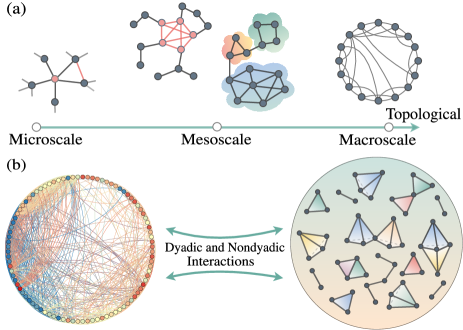
Figure 1: Various topological scales and interactions between multiple elements in a complex network. (a) Complex networks can be analyzed at various topological scales ranging from individual nodes (microscale) to the whole network (macroscale). In between the two scales, there is a mesoscale, where we can observe patterns of collectives, cores, and peripheries. (b) Complex network is a representation of a complex system having dyadic and nondyadic interactions between its elements. The interactions can be represented as simplices such as segments (for dyadic interactions), filled triangles, or filled tetrahedrons (for nondyadic interactions involving three or four elements), and so on.

II Method

II.1 Scale-variant topological features

Let $\mathcal{G}$ be an undirected weighted network with $N$ nodes, $v_{1},\ldots,v_{N}$, and assume that there is a single random walker moving randomly between the nodes in continuous time. When the walker is located at $v_{i}$, we assume the walker to move to the neighboring node $v_{j}$ at a transition rate $w_{ij}/W_{i}$, where $w_{ij}\geq 0$ represents the weight of the edge from $v_{i}$ to $v_{j}$ ($i,j\in\{1,2,\ldots,N\}$) and $W_{i}=\sum_{j=1}^{N}w_{ij}$. Herein, if there is no edge between $v_{i}$ and $v_{j}$, then $w_{ij}=0$. Now, let $p_{\mathcal{G},k}(\tau|i)$ denote the probability of a random walker on $v_{k}$ at time $\tau$ that starts from $v_{i}$. The probability distribution vector, $\bm{p}_{\mathcal{G}}(\tau|i)=\left[p_{\mathcal{G},1}(\tau|i),\ldots,p_{\mathcal{G},N}(\tau|i)\right]$, is given based on the solution of the Kolmogorov forward equation De Domenico (2017):

$$\dfrac{d\bm{p}_{\mathcal{G}}(\tau|i)}{d\tau}=-\bm{p}_{\mathcal{G}}(\tau|i)\bm{L}^{\text{rw}}_{\mathcal{G}}.$$ (1)

Here, $\bm{L}^{\text{rw}}_{\mathcal{G}}$ is the random walk Laplacian whose components $l_{ij}$ ($i,j\in\{1,2,\ldots,N\}$) are given by,

$$l_{ij}=\begin{cases}1&\textrm{ if $i=j$ and $W_{i}\neq 0$}\\ -w_{ij}/W_{i}&\textrm{ if $i\neq j$ and $v_{i}$ is adjacent to $v_{j}$}\\ 0&\textrm{ otherwise.}\\ \end{cases}$$ (2)

The solution for Eq. (1) is $\bm{p}_{\mathcal{G}}(\tau|i)=\bm{u}_{i}\exp(-\tau\bm{L}^{\text{rw}}_{\mathcal{G}})$, where $\bm{u}_{i}=\left[0,\ldots,0,1,0,\ldots,0\right]$ with its $i$-th element being equal to 1; the others are equal to 0 ($i\in\{1,2,\ldots,N\}$).

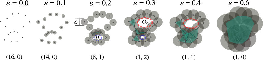
Figure 2: An exemplary of Vietoris–Rips filtration constructed from a point cloud. A union of balls of radius $\varepsilon/2$ centered at each point is considered. Topological structure changes are tracked, such as the merging of connected components or clusters, and the emergence and disappearance of loops or circular holes present in the space with increasing $\varepsilon$ from {0.0, 0.1, 0.2, 0.3, 0.4, 0.6}. For instance, the blue loop $\Omega_{1}$ appears at $\varepsilon=0.2$ then disappears at $\varepsilon=0.4$, whereas the red loop $\Omega_{2}$ appears at $\varepsilon=0.3$ then disappears at $\varepsilon=0.6$. For each $\varepsilon$, the number of connected components and the number of loops are listed underneath.

At each timescale $\tau$, we consider mapping $\chi_{\tau}$ from the set $V_{\mathcal{G}}=\{v_{1},v_{2},\ldots,v_{N}\}$ of nodes in $\mathcal{G}$ to the Euclidean space $\mathbb{R}^{N}$ such that,

$$\chi_{\tau}:\quad V_{\mathcal{G}} \longrightarrow\mathbb{R}^{N}$$

$$v_{i} \longmapsto\bm{p}_{\mathcal{G}}(\tau|i)\quad(i=1,2,\ldots,N).$$ (3)

The mapped point $\bm{p}_{\mathcal{G}}(\tau|i)$ of nodes $v_{i}$ represents the probability on all nodes at time $\tau$ of a random walker that starts from $v_{i}$. Therefore, $\bm{p}_{\mathcal{G}}(\tau|i)$ can reflect the interaction between $v_{i}$ and other nodes at $\tau$-scale, and characterize the structural role of node $v_{i}$ with multi-resolutions when $\tau$ varies. The shape of the point cloud $P_{\mathcal{G}}(\tau)=\{\bm{p}_{\mathcal{G}}(\tau|1),\ldots,\bm{p}_{\mathcal{G}}(\tau|N)\}$ provides valuable insights into the dyadic and nondyadic interactions between nodes, and into the structural property of $\mathcal{G}$ at $\tau$-scale. Moreover, the distance between two mapped points in $P_{\mathcal{G}}(\tau)$ is relatively small if there are many paths connecting two original nodes in $\mathcal{G}$. The nodes that belong to the same community or cluster in the network tend to form a group of close points in $P_{\mathcal{G}}(\tau)$.

Information on the shape of the point cloud can be obtained quantitatively using the method of persistent homology from computational topology Edelsbrunner et al. (2002); Zomorodian and Carlsson (2005); Carlsson (2009); Edelsbrunner and Harer (2010). The idea is to construct from $P_{\mathcal{G}}(\tau)$ the $\varepsilon$-scale Vietoris–Rips complex model $V_{\textup{R}}(P_{\mathcal{G}}(\tau),\varepsilon)$, which is a set of simplices built with a nonnegative threshold $\varepsilon$ Kaczynski et al. (2006). Here, every collection of $n+1$ affinely independent points in $P_{\mathcal{G}}(\tau)$ forms an $n$-simplex in $V_{\textup{R}}(P_{\mathcal{G}}(\tau),\varepsilon)$ if the pairwise distance between the points is less than or equal to $\varepsilon$. To build the Vietoris–Rips complex model, we consider a union of balls of radius $\varepsilon/2$ centered at each point in $P_{\mathcal{G}}(\tau)$ (Fig. 2). Each simplex is built over a subset of points if the balls intersect between every pair of points. These simplices can represent the nondyadic interactions of nodes at $\tau$-scale. In turn, the constructed complex $V_{\textup{R}}(P_{\mathcal{G}}(\tau),\varepsilon)$ provides information on the topological structure of $P_{\mathcal{G}}(\tau)$ associated with $\varepsilon$. Now, starting with $\varepsilon=0$, the complex contains only the $0$-simplices, i.e., the discrete points. As $\varepsilon$ increases, connections exist between the points, enabling us to obtain a sequence of embedded complexes called filtration with edges ($1$-simplices), and triangular faces ($2$-simplices) are included into the complexes. Moreover, if $\varepsilon$ becomes considerably large, all the points gets connected with each other, whereby no useful information can be conveyed.

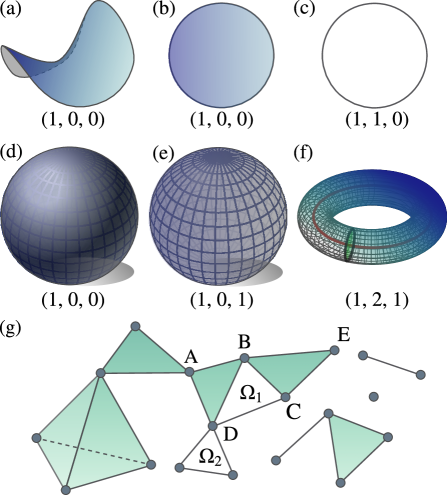
Figure 3: (a)–(f) Sample manifolds with the number of zero-, one-, and two-dimensional holes listed underneath. (a) The connected component is a zero-dimensional hole. (b)(c) A one-dimensional hole is obtained by puncturing a disk. (d)(e) A two-dimensional hole is obtained by emptying the inside of a ball. (f) Two one-dimensional holes are illustrated as two circles in a torus. (g) Example of a simplicial complex containing 19 points (0-simplices), 24 edges (1-simplices), eight triangular faces (2-simplices), and one filled tetrahedron (3-simplices). There are two one-dimensional holes $\Omega_{1}$ and $\Omega_{2}$ in the complex. In this example, all loops $B\rightarrow C\rightarrow D\rightarrow B$, $A\rightarrow B\rightarrow C\rightarrow D\rightarrow A$, $B\rightarrow E\rightarrow C\rightarrow D\rightarrow B$, and $A\rightarrow B\rightarrow E\rightarrow C\rightarrow D\rightarrow A$ are 1-cycles because they are closed 1-chains, that is, the closed collection of edges (1-simplices). Each cycle is not a boundary of any 2-chain (collection of triangular faces); thus, it characterizes a one-dimensional hole. Note that these cycles characterize the same hole, $\Omega_{1}$, because the difference between the two of cycles is the boundary of a 2-chain.

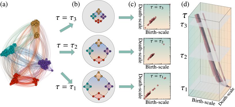
Figure 4: (a) An undirected network comprising four clusters with more connections within intra-clusters than between inter-clusters. (b) For each $\tau$, the nodes are mapped onto a point cloud such that the distances of the mapped points of the nodes in the same clusters are smaller than those between the nodes belonging to different clusters. These distances decrease as $\tau$ increases with $\tau_{1}<\tau_{2}<\tau_{3}$. (c) The topological features at each $\tau$ characterize the shape of the point cloud. These features are displayed as a two-dimensional persistence diagram at each $\tau$. (d) The scale-variant topological features, i.e., the three-dimensional persistence diagram, are obtained by integrating two-dimensional diagrams at varying $\tau$. The birth-scale and death-scale axes of the diagrams are represented at the logarithmic scale.

Persistent homology tracks the variation of topological structures over the filtration. We refer to the topological structures, i.e., “holes” in high-dimensional data, as connected components, tunnels or loops (e.g., a circle of torus), cavities or voids (e.g., the space enclosed by a sphere), and so on. In persistent homology, a hole is identified via the cycle that surrounds it. In a given manifold, a cycle is a closed submanifold, and a boundary is a cycle that is also the boundary of a submanifold. Holes correspond to cycles that are not themselves boundaries. For instance, a disk is a two-dimensional surface with a one-dimensional boundary (i.e., a circle). If we puncture the disk, we obtain a one-dimensional hole that is enclosed by the circle, which is no longer a boundary [Fig. 3(b)(c)]. Similarly, a filled ball is a three-dimensional object with a two-dimensional boundary (i.e., a surface sphere). If we empty the inside of the ball, we obtain a two-dimensional hole that is enclosed by the surface sphere, which is no longer a boundary [Fig. 3(d)(e)]. Based on these observations, we can describe and classify holes in the simplicial complex according to the cycles that enclose holes. Given a simplicial complex, we define an $n$-chain as a collection of $n$-simplices in the complex. Therefore, in a simplicial complex, we can define an $n$-cycle as a closed $n$-chain and an $n$-boundary as an $n$-cycle, which is also the boundary of an $(n+1)$-chain. Here, a $0$-cycle is a connected component, a $1$-cycle is a closed loop, and a $2$-cycle is a shell. For instance, in Fig. 3(g), all loops $A\rightarrow B\rightarrow D\rightarrow A$, $B\rightarrow C\rightarrow D\rightarrow B$, and $A\rightarrow B\rightarrow C\rightarrow D\rightarrow A$ are 1-cycles because they are the closed collection of edges (1-simplices). Furthermore, the loop $A\rightarrow B\rightarrow D\rightarrow A$ is a 1-boundary because it bounds a triangular face (2-simplex). An $n$-dimensional hole corresponds to an $n$-cycle that is not a boundary of any $(n+1)$-chain in the simplicial complex. For instance, as illustrated in Fig. 3(g), the loops $B\rightarrow C\rightarrow D\rightarrow B$ and $A\rightarrow B\rightarrow C\rightarrow D\rightarrow A$ characterize one-dimensional holes because these loops are 1-cycles but are themselves not 1-boundaries. Moreover, two $n$-cycles characterize the same hole when together they bound an $(n+1)$-chain (i.e., their difference is an $n$-boundary). Intuitively, the connected components can be considered as zero-dimensional holes, the loops and tunnels as one-dimensional holes, and the cavities and voids as two-dimensional holes.

We consider the emergence and disappearance of holes in the Vietoris–Rips filtration of $P_{\mathcal{G}}(\tau)$ as topological features for the complex network $\mathcal{G}$ at $\tau$-scale. Such features can be observed using multi-set points in a two-dimensional persistence diagram, $D^{(2)}_{(l),\tau}(\mathcal{G})$, which is calculated for $l$-dimensional holes. In this diagram, each point $(b,d)$ denotes a hole that appears at the birth-scale, $\varepsilon=b$, and disappears at the death-scale, $\varepsilon=d$ (see Appendix A). Observing the above-defined features, i.e., the two-dimensional persistence diagrams with varying $\tau$ can provide insights into the variation of topological structures, thereby reflecting the variation of topological scales in the network. For instance, the persistence diagrams of zero-dimensional and one-dimensional holes contain information on clusters, connected components, or loops in the point cloud $P_{\mathcal{G}}(\tau)$, and thus lead to an understanding of the formation of communities and loops in the network at the $\tau$-scale. We construct scale-variant topological features by regarding $\tau$ as a variable parameter rather than as a single fixed value.

In Fig. 4(a), we consider an undirected network that comprises four clusters with more intra-cluster connections than inter-cluster ones. Pairwise distances of the mapped points of the nodes belonging to the same clusters are smaller than the distances between the nodes belonging to different clusters. These distances decrease as values of $\tau$ increase [Fig. 4(b)]. In the point cloud, the hole patterns appear with different sizes in different groups of points as $\tau$ varies. We obtain the scale-variant topological features that reflect the variation of topological scales by considering the two-dimensional persistence diagrams with the varying $\tau$. Consider $\tau$ in a set $\mathcal{T}=\{\tau_{1},\tau_{2},...,\tau_{K}\}$, where $0<\tau_{1}<\tau_{2}<\cdots<\tau_{K}$ are predefined or sampled values from the continuous domain of timescales. The scale-variant topological features, i.e., the three-dimensional persistence diagram of $l$-dimensional holes for network $\mathcal{G}$, are defined by $D^{(3)}_{(l)}(\mathcal{G})=\{(b,d,\tau)\mid(b,d)\in D^{(2)}_{(l),\tau}(\mathcal{G}),\tau\in\mathcal{T}\}$ [Fig. 4(d)].

II.2 Robustness of scale-variant topological features

We show that the scale-variant topological features are robust with respect to some perturbations of the network. To describe this robustness, we use the bottleneck distance, $d^{(3)}_{\textup{B},\xi}$, a metric structure introduced in Ref. Tran and Hasegawa (2019) for comparing three-dimensional persistence diagrams (see Appendix B). Herein, $\xi$ is a positive rescaling coefficient introduced to adjust the scale difference between the pointwise distance and time. We consider two undirected networks $\mathcal{G}$ and $\mathcal{H}$ with the same number of nodes. Based on Refs. Golub and Van Loan (2012); Chazal et al. (2014), we can prove that the upper limit of the bottleneck distance between $D_{(l)}^{(3)}(\mathcal{G})$ and $D_{(l)}^{(3)}(\mathcal{H})$ is governed by the matrix 2-norm of the difference between $\bm{L}^{\text{rw}}_{\mathcal{G}}$ and $\bm{L}^{\text{rw}}_{\mathcal{H}}$ (see Appendix B):

$$d^{(3)}_{\textup{B},\xi}(D^{(3)}_{(l)}(\mathcal{G}),D^{(3)}_{(l)}(\mathcal{H}))\leq 2\tau_{K}\|\bm{L}^{\text{rw}}_{\mathcal{G}}-\bm{L}^{\text{rw}}_{\mathcal{H}}\|_{2}.$$ (4)

Herein, $\|\bm{A}\|_{2}$ denotes the matrix 2-norm of matrix $\bm{A}$. The inequality of Eq. (4) indicates that our scale-variant topological features are robust with respect to the perturbations applied to the random walk Laplacian matrix. Therefore, these features can be used as discriminative features for characterizing networks.

II.3 Kernel method for scale-variant topological features

In the statistical-learning tasks, many learning algorithms require an inner product between the data in the vector form. Because the space of three-dimensional persistence diagrams is not a vector space, we deem it not straightforward to use the scale-variant topological features in the statistical-learning tasks. This problem can be mitigated through the use of a feature map $\Phi$ from the positive-definite kernel, which maps the scale-variant topological features to a space called kernel-mapped feature space $H_{b}$ where we can define the inner product Tran and Hasegawa (2019). In general, choosing the explicit form of mapping a persistence diagram $E$ to $\Phi_{E}$ in the kernel-mapped feature space is not discernible. Nonetheless, we can use a kernel function to compute the inner product in the kernel-mapped feature space, leaving the mapping function and the kernel-mapped feature space completely implicit.

Given a positive bandwidth $\sigma$ and a positive rescaling coefficient $\xi$ introduced to adjust the scale difference between the point-wise distance and time (see Appendix C), based on Refs. Reininghaus et al. (2015); Tran and Hasegawa (2019), we define the kernel $\mathcal{K}_{\sigma,\xi}$ between two three-dimensional persistence diagrams, $E$ and $F$, as

$$\mathcal{K}_{\sigma,\xi}(E,F)=\frac{1}{\sigma\sqrt{2\pi}}\sum_{\bm{q}^{(1)}\in E\atop\bm{q}^{(2)}\in F}\left(e^{-\frac{d_{\xi}^{2}(\bm{q}^{(1)},\bm{q}^{(2)})}{2\sigma^{2}}}-e^{-\frac{d_{\xi}^{2}(\bm{q}^{(1)},\bar{\bm{q}}^{(2)})}{2\sigma^{2}}}\right),$$ (5)

where $d^{2}_{\xi}(\bm{q}^{(1)},\bm{q}^{(2)})=|b_{1}-b_{2}|^{2}+|d_{1}-d_{2}|^{2}+\xi^{2}|\tau_{1}-\tau_{2}|^{2}$, $d^{2}_{\xi}(\bm{q}^{(1)},\bar{\bm{q}}^{(2)})=|b_{1}-d_{2}|^{2}+|d_{1}-b_{2}|^{2}+\xi^{2}|\tau_{1}-\tau_{2}|^{2}$, with $\bm{q}^{(1)}=\left(b_{1},d_{1},\tau_{1}\right)$ and $\bm{q}^{(2)}=\left(b_{2},d_{2},\tau_{2}\right),\bar{\bm{q}}^{(2)}=\left(d_{2},b_{2},\tau_{2}\right)$. In our experiments, we use the normalized version of the kernel, which is calculated as

$$\mathcal{K}_{\sigma,\xi}(E,F)\leftarrow\mathcal{K}_{\sigma,\xi}(E,F)/\sqrt{\mathcal{K}_{\sigma,\xi}(E,E)\mathcal{K}_{\sigma,\xi}(F,F)}.$$ (6)

Because Eq. $\eqref{eqn:kernel}$ and Eq. $\eqref{eqn:kernel:label}$ define the positive-definite kernels in the set of three-dimensional persistence diagrams Tran and Hasegawa (2019), according to Moore–Aronszajn’s theorem Aronszajn (1950), there exists a mapping function $\Phi$ such that the inner product $\langle\Phi_{E},\Phi_{F}\rangle_{H_{b}}$ between $\Phi_{E}$ and $\Phi_{F}$ in the kernel-mapped feature space $H_{b}$ is $\mathcal{K}_{\sigma,\xi}(E,F)$. Therefore, we can use the explicit form of inner product $\langle\Phi_{E},\Phi_{F}\rangle_{H_{b}}$ in the statistical-learning tasks.

Furthermore, we can use the above-defined kernel to estimate the transition points with respect to the topological structure in the series of networks $\mathcal{G}_{1},\mathcal{G}_{2},\ldots,\mathcal{G}_{M}$. Consider a collection of diagrams $\mathcal{D}_{(l)}=\{D_{(l),1}^{(3)},D_{(l),2}^{(3)},\ldots,D_{(l),M}^{(3)}\}$, where $D_{(l),i}^{(3)}$ is the three-dimensional persistence diagram of $l$-dimensional holes for network $\mathcal{G}_{i}$ ($i=1,2,\ldots,M)$. Here, we define the transition with respect to the topological structure in $\mathcal{G}_{1},\mathcal{G}_{2},\ldots,\mathcal{G}_{M}$ as they abruptly change at given unknown instants (change-points) in $\mathcal{D}_{(l)}$. We use the kernel change-point detection method Harchaoui et al. (2009) to solve the change-point regression problem with $\Phi_{D^{(3)}_{(l),1}},\Phi_{D^{(3)}_{(l),2}},\ldots,\Phi_{D^{(3)}_{(l),M}}$. Given an index $s$ ($1<s\leq M)$, we calculate the kernel Fisher discriminant ratio $\kappa_{M,s}(\mathcal{D}_{(l)})$, which is a statistical quantity to measure the dissimilarity between two classes assumptively defined by two sets of diagrams having index before and from $s$ (see Appendix D). Here, the index $s$ achieving the maximum of $\kappa_{M,s}(\mathcal{D}_{(l)})$ corresponds to the estimated transition point.

III Results

III.1 Understanding variations of the parameters of network models

We now investigate how the scale-variant topological features can reflect variations of the parameters of network models. We generate networks using Girvan–Newman (GN) Newman and Girvan (2004), Lancichinetti–Fortunato–Radicchi (LFR) Lancichinetti et al. (2008); Lancichinetti and Fortunato (2009), Watts–Strogatz (WS) Watts and Strogatz (1998), Erdős–Rényi (ER) Erdős and Rényi (1959), Lancichinetti–Fortunato–Radicchi with hierarchical structure (LFR–H) Lancichinetti et al. (2009), and Sales–Pardo (SP) Sales-Pardo et al. (2007) models. We focus on the model parameters that represent the topological scale of these networks, such as the ratio $r$ between the probability of inter- ($p_{\text{out}}$) and intra-community links ($p_{\text{in}}$) (GN), mixing rate $\mu$ (LFR), rewiring probability $\beta$ (WS), pair-link probability $p_{\text{link}}$ (ER), mixing rate $\mu_{\text{macro}}$ for macrocommunities (LFR–H), and $\rho$, which estimates the separations between topological scales in the SP model. The model parameters are varied as $r=p_{\text{out}}/p_{\text{in}}=0.01,0.02,\ldots,1.0$; $\mu=0.01,0.02,\ldots,1.0$; $\beta=0.00,0.01,\ldots,1.0$; $p_{\text{link}}=0.020,0.021,\ldots,0.1$; $\mu_{\text{macro}}=0.01,0.02,\ldots,0.2$ and; $\rho=0.05,0.10,\ldots,2.0$. We generate 10 network realizations for each of the models GN, LFR, WS, ER, and SP, and 20 network realizations for the LFR–H model at each value of the corresponding model parameter. There are 128 nodes in the GN, LFR, WS, and ER networks, 300 nodes in each LFR–H network, and 640 nodes in each SP network.

We compute three-dimensional persistence diagrams for one-dimensional holes with $\tau_{1}=1,\tau_{2}=2,\ldots,\tau_{100}=100$, and then calculate the kernel defined in Eq. (5) for the collection of generated networks in each model. Figure 5 shows the principal components projections from the kernel-mapped feature space of each model, at which the points with different colors represent the networks generated from different values of the model parameters. In WS, ER, LFR–H, and SP models, the scale-variant topological features reflect a variation of the parameters associated with the topological scales mainly that the points located at different positions have different colors [Fig. 5(c)–(f)]. In GN and LFR models, there are variations in the topological scales of the network as $r$ and $\mu$ vary from 0 (four separate groups) to 1 (a purely random graph). Using the kernel Fisher discriminant ratio calculated for the series of persistence diagrams, we obtain the transition with respect to the topological structure at $r=0.12$ and $\mu=0.26$ for the series of networks obtained at increasing $r$ and $\mu$  (Fig. 6). These values correspond to the boundaries between the identifiable phases, where parameters can be identified from the kernel-mapped feature space and the non-identifiable phases [Fig. 5(a)–(b)].

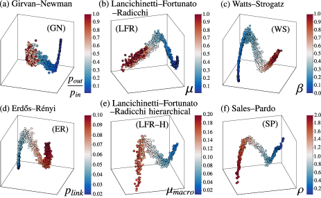
Figure 5: Principal components projection from the kernel-mapped feature space of the scale-variant topological features in each network model. Points with different colors represent networks generated from different values of the model parameters. Networks are generated from (a) Girvan–Newman (GN), (b) Lancichinetti–Fortunato–Radicchi (LFR), (c) Watts–Strogatz (WS), (d) Erdős–Rényi (ER), (e) Lancichinetti–Fortunato–Radicchi hiearchical (LFR–H), and (f) Sales–Pardo (SP) models. Parameters for these models vary as follows: $r=p_{\text{out}}/p_{\text{in}}=0.01,0.02,\ldots,1.0$ (GN); $\mu=0.01,0.02,\ldots,1.0$ (LFR); $\beta=0.00,0.01,\ldots,1.0$ (WS); $p_{\text{link}}=0.020,0.021,\ldots,0.1$ (ER); $\mu_{\text{macro}}=0.01,0.02,\ldots,0.2$ (LFR–H) and; $\rho=0.05,0.10,\ldots,2.0$ (SP).

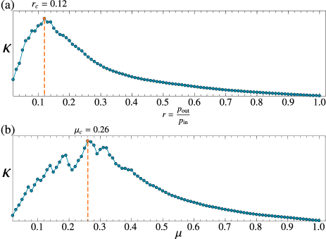
Figure 6: Kernel Fisher discriminant ratio $\kappa$ estimated for the series of (a) Girvan–Newman networks and (b) Lancichinetti–Fortunato–Radicchi networks. The transition point is detected with respect to the topological structure of networks from the series of persistence diagrams for one-dimensional holes obtained when $r=p_{\text{out}}/p_{\text{in}}$ is increased as $r_{1}=0.01,r_{2}=0.02,\ldots,r_{100}=1.0$ (for Girvan–Newman networks), and $\mu$ is increased as $\mu_{1}=0.01,\mu_{2}=0.02,\ldots,\mu_{100}=1.0$ (for Lancichinetti–Fortunato–Radicchi networks). The maximum value of $\kappa$ is marked with the orange point of the dashed line. The transition point is the value of the parameter that achieves the maximum value of $\kappa$. The transition points are obtained as $r_{c}=0.12$ (for Girvan–Newman networks) and $\mu_{c}=0.26$ (for Lancichinetti–Fortunato–Radicchi networks).

III.2 Identification of network models

Figure 7: Networks from Girvan–Newman, Lancichinetti–Fortunato–Radicchi, and Watts–Strogatz models are generated with labels denoted by GN-org, LFR-org, and WS-org, respectively; their corresponding configuration networks labels are denoted by GN-conf, LFR-conf, and WS-conf. (a) The kernel principal components projection of the scale-variant topological features for these networks. (b)(c) Variation of high-order features, i.e., degree assortativity coefficient, maximum modularity, and average clustering coefficient for (b) all generated networks, and (c) configuration networks. The different colors represent the networks generated from different models.

Here we show that the scale-variant topological features can classify the networks generated from different models, even if they have similar global statistical measures. We study the configuration model in Ref. Newman et al. (2001), which generates random networks (known as configuration networks) having the same sequences of node degrees as a given network. The labels of the networks generated from GN, LFR, and WS models are denoted by GN-org, LFR-org, and WS-org, respectively, while their corresponding configuration networks labels are denoted by GN-conf, LFR-conf, and WS-conf. We compute the three-dimensional persistence diagrams for one-dimensional holes of these networks with timescale values $\tau_{1}=1,\tau_{2}=2,\ldots,\tau_{100}=100$. Accordingly, we calculate the kernel for these diagrams, then perform three-dimensional projections of the principal components from the kernel-mapped feature space [Fig. 7(a)]. Here, points with different colors represent networks generated from different models. In Fig. 7(a), the points appear to be distinguishable by their colors, thus, we can conclude that the scale-variant topological features can characterize the differences with respect to the topological structure between networks, and even between configuration networks generated from different models.

While the node degree distribution in a configuration network is the same as the given network, the topological correlations between the nodes are destroyed. Therefore, we investigate conventional higher-order features of the network, such as the degree assortativity coefficient, the average clustering coefficient, and the maximum modularity obtained via Louvain heuristic Blondel et al. (2008); Newman and Girvan (2004). Figure 7(b) highlights the variation of these features in our generated networks. Specifically in Fig. 7(b), the points with corresponding labels GN-org, LFR-org, and WS-org appear to be distinguishable with others, thus, it becomes easy to distinguish between networks generated from different models and between a given network with its corresponding configuration network. However, if we look at the variation of these features for configuration networks [Fig. 7(c)], we note that the conventional higher-order features of the network cannot capture the apparent differences in topological structure between the configuration networks, even when their corresponding original networks are generated from different mechanics models. In contrast with this observation and as highlighted in Fig. 7(a), the scale-variant topological features can provide a better representation of the topological structure of networks.

Accordingly, we quantify to what extent the scale-variant topological features identify the networks generated from different models. We employ the scale-variant method, which uses the scale-variant topological features to classify networks into six labels, namely, GN-org, LFR-org, WS-org, GN-conf, LFR-conf, and WS-conf. We randomly split 10 networks generated at each value of the model parameters into two, i.e., five networks for training and five for testing, and apply the support vector machine Bishop (2006) for classification in the kernel-mapped feature space. Figure 8(a) depicts the average normalized confusion matrix over 100 random splits, where the row and column labels are the predicted and true labels, respectively. Figure 8(a) shows a reasonably high accuracy for identifying the networks generated from different models with the following labels: GN-org ($99.2\%$), LFR-org ($99.2\%$), WS-org ($99.4\%$), GN-conf ($94.8\%$), LFR-conf ($99.4\%$), and WS-conf ($96.6\%$). This result demonstrates that the scale-variant topological features can reflect well on the behaviors of these network models.

Figure 8: Classification of networks generated from Girvan–Newman, Lancichinetti–Fortunato–Radicchi, and Watts–Strogatz models, with labels denoted by GN-org, LFR-org, and WS-org, respectively; their corresponding configuration networks labels are denoted by GN-conf, LFR-conf, and WS-conf. (a) Average normalized confusion matrix of the scale-variant method over 100 random train-test splits of the data. The 10 networks generated at each value of the model parameters are split into two, with five networks for training and the other five for testing. (b) Average accuracies (%) of the classification methods over 100 random train-test splits at each proportion of the training data (bold lines). The shaded areas indicate the confidence intervals of one standard deviation calculated using the same ensemble of runs.

To highlight the benefits of the scale-variant method, we compare it with the other conventional methods using common network measures Freeman (1978); Latora and Marchiori (2001); Newman (2002); Costa et al. (2007); Brandes (2008), well-recognized graph kernels Sugiyama et al. (2017), and topological features calculated at an average fixed topological scale. We describe the common network measures in Appendix E as well as the graph kernels that are based on random walks (KStepRW, GeometricRW, ExponentialRW) Kashima et al. (2003); Gärtner et al. (2003), paths (ShortestPath) Borgwardt and Kriegel (2005), limited-sized subgraphs (Graphlet) Borgwardt et al. (2007), and subtree patterns (Weisfeiler–Lehman Shervashidze et al. (2011)) in Appendix F. Moreover, we consider two variations of topological features evaluated at an average fixed topological scale to show the advantages of using variable timescales. Also, instead of using a particular timescale, we use the scale-average and the scale-norm-average methods to preserve the geometrical persistence of the point cloud. The former uses the topological features extracted from the average distance matrix $\bm{\Delta}_{\text{avg}}=(1/K)\sum_{i=1}^{K}\bm{\Delta}_{\tau_{i}}$, whereas the latter uses the features from the average normalized distance matrix $\tilde{\bm{\Delta}}_{\text{avg}}=(1/K)\sum_{i=1}^{K}\tilde{\bm{\Delta}}_{\tau_{i}}$ De Domenico (2017). Herein, $\bm{\Delta}_{\tau_{i}}$ denotes the distance matrix of pairwise Euclidean distances between points in $P_{\mathcal{G}}(\tau_{i})$, whereas $\tilde{\bm{\Delta}}_{\tau_{i}}$ is obtained by dividing $\bm{\Delta}_{\tau_{i}}$ by its maximum element. We randomly split the 10 networks generated at each value of the model parameters into proportions for training and for testing, and employ the support vector machine as the classifier to both the common network measures and the kernel-mapped feature space. We compute the average classification accuracy over 100 random splits at different proportions of the training data. Figure 8(b) depicts the performance of the methods with accuracies greater than 70%, mainly illustrating that the scale-variant method outperforms the other methods in terms of classification accuracy. Moreover, the scale-variant method is shown to achieve approximately 97% of accuracy, even with a small size of the training dataset, e.g., only 10$\%$ of all the data, whereas the other methods yielded accuracies of at most 84%. These results validate the effectiveness and the reliability of our scale-variant method in capturing the differences between network structures. The source code used in our experiments is publicly available on GitHub Tran et al. .

III.3 Classification of the real-world network data

Next, we apply the scale-variant topological features to the classification of chemoinformatics network datasets (MUTAG, BZR, COX2, DHFR, FRANKENSTEIN, NCI1, NCI109), bioinformatics dataset (PROTEIN), and large real-world social network datasets, such as movie collaboration networks (IMDB–BINARY, IMDB–MULTI), scientific collaboration networks (COLLAB), and networks obtained from online discussion threads on Reddit (REDDIT–BINARY, REDDIT–MULTI–5K) Debnath et al. (1991); Sutherland et al. (2003); Kazius et al. (2005); Borgwardt et al. (2005); Wale et al. (2008); Orsini et al. (2015); Yanardag and Vishwanathan (2015); Kersting et al. (2016). The aggregate statistics for these datasets is provided in Table 1. We compute three-dimensional persistence diagrams with $\tau_{1}=1,\ldots,\tau_{50}=50$, and use the multiple kernel learning method Cortes et al. (2012) to learn the linear combination of the normalized kernels for zero-dimensional and one-dimensional holes. Subsequently, we compare our scale-variant method with methods employing the common network measures and the scale-average and scale-norm-average methods. Likewise, we compare the scale-variant method with many state-of-the-art algorithms in classifying graphs and networks as follows: (i) random walk kernels based on matching walks in two graphs (KStepRW, GeometricRW, ExponentialRW) Kashima et al. (2003); Gärtner et al. (2003), (ii) the shortest path kernel (ShortestPath) Borgwardt and Kriegel (2005), (iii) the graphlet count kernel (Graphlet) Borgwardt et al. (2007), (iv) the Weisfeiler–Lehman subtree kernel (Weisfeiler–Lehman) Shervashidze et al. (2011), (v) the deep graph kernel (DGK) Yanardag and Vishwanathan (2015), (vi) the PATCHY-SAN convolutional neural network (PSCN) Niepert et al. (2016), and (vii) the graph kernel based on return probabilities of random walks (RetGK) Zhang et al. (2018). Here, in order to make a fair comparison with these methods, as presented in the literature Ref. Zhang et al. (2018), we apply the support vector machine Bishop (2006) as the classifier in the kernel-mapped feature space. Moreover, we perform 10-fold cross-validations, where a single 10-fold is created by randomly shuffling the dataset, and then splitting it into 10 different parts (folds) of equal size. In every single 10-fold, we use nine folds for training and one for testing and averaging of the classification accuracy of the test set obtained throughout the folds. To reduce the variance of the accuracy due to the splitting of data, we repeat the whole process of cross-validation for 10 times, and then report the average and standard deviation of the classification accuracies.

Table 1: Summary statistics of the real-world network datasets.

Dataset	Type of networks	Number of networks	Number of classes	Number of networks in each class	Avg. number of nodes	Avg. number of edges
MUTAG	Chemoinformatics	188	2	(63,125)	17.93	19.79
BZR	Chemoinformatics	405	2	(319, 86)	35.75	38.36
COX2	Chemoinformatics	467	2	(365, 102)	41.22	43.45
DHFR	Chemoinformatics	756	2	(295, 461)	42.43	44.54
FRANKENSTEIN	Chemoinformatics	4337	2	(2401, 1936)	16.90	17.88
NCI1	Chemoinformatics	4110	2	(2053, 2057)	29.87	32.30
NCI109	Chemoinformatics	4127	2	(2048, 2079)	29.68	32.13
PROTEINS	Bioinformatics	1113	2	(663, 450)	39.06	72.82
IMDB–BINARY	Social	1000	2	(500, 500)	19.77	96.53
IMDB–MULTI	Social	1500	3	(500, 500, 500)	13.00	65.94
COLLAB	Social	5000	3	(2600, 775, 1625)	74.49	2457.78
REDDIT–BINARY	Social	2000	2	(1000, 1000)	429.63	497.75
REDDIT–MULTI–5K	Social	4999	5	(1000, 1000, 1000, 1000, 999)	508.52	594.87

Table 2: Average and standard deviation (mean$\pm$sd) of the classification accuracy (%) for social network datasets IMDB–BINARY, IMDB–MULTI, COLLAB, REDDIT–BINARY, and REDDIT–MULTI–5K. These social network datasets contain networks that do not have information such as labels and attributes of nodes. In each dataset, the best and the second-best scores are colored in dark pink and light pink, respectively. The notation $(*)$ indicates that the kernel computation with the implementation in Sugiyama et al. (2017) is not completed after 72h.

Method	IMDB–BINARY	IMDB–MULTI	COLLAB	REDDIT– BINARY	REDDIT– MULTI–5K
Scale-variant	74.2 $\pm$ 0.9	49.9 $\pm$ 0.3	79.6 $\pm$ 0.3	87.8 $\pm$ 0.3	53.1 $\pm$ 0.2
Scale-average	67.7 $\pm$ 0.8	44.9 $\pm$ 0.4	71.4 $\pm$ 0.1	79.8 $\pm$ 0.3	51.5 $\pm$ 0.2
Scale-norm-average	70.2 $\pm$ 0.7	44.9 $\pm$ 0.4	62.6 $\pm$ 0.1	73.9 $\pm$ 0.2	48.7 $\pm$ 0.3
CommonMeasures	72.0 $\pm$ 0.2	44.9 $\pm$ 0.3	75.2 $\pm$ 0.1	85.7 $\pm$ 0.3	56.6 $\pm$ 0.2
KStepRW	60.0 $\pm$ 0.8	43.8 $\pm$ 0.7	$(*)$	$(*)$	$(*)$
GeometricRW	67.0 $\pm$ 0.8	45.2 $\pm$ 0.4	$(*)$	$(*)$	$(*)$
ExponentialRW	65.2 $\pm$ 1.1	43.1 $\pm$ 0.4	$(*)$	$(*)$	$(*)$
ShortestPath	58.2 $\pm$ 1.0	42.0 $\pm$ 0.6	58.5 $\pm$ 0.2	81.9 $\pm$ 0.1	49.0 $\pm$ 0.1
Graphlet	65.9 $\pm$ 1.0	43.9 $\pm$ 0.4	72.8 $\pm$ 0.3	77.3 $\pm$ 0.2	41.0 $\pm$ 0.2
Weisfeiler–Lehman	70.8 $\pm$ 0.5	49.8 $\pm$ 0.5	74.8 $\pm$ 0.2	68.2 $\pm$ 0.2	51.2 $\pm$ 0.3
DGK	67.0 $\pm$ 0.6	44.6 $\pm$ 0.5	73.1 $\pm$ 0.3	78.0 $\pm$ 0.4	41.3 $\pm$ 0.2
PSCN	71.0 $\pm$ 2.3	45.2 $\pm$ 2.8	72.6 $\pm$ 2.2	86.3 $\pm$ 1.6	49.1 $\pm$ 0.7
RetGK	71.9 $\pm$ 1.0	47.7 $\pm$ 0.3	81.0 $\pm$ 0.3	92.6 $\pm$ 0.3	56.1 $\pm$ 0.5

Table 3: Average and standard deviation (mean$\pm$sd) of the classification accuracy (%) for chemoinformatics and bioinformatics datasets MUTAG, BZR, COX2, DHFR, FRANKENSTEIN, PROTEINS, NCI1, and NCI109. Presented is only a comparison of the methods using the connectivity between nodes. In each dataset, the best and the second-best scores are colored in dark pink and light pink, respectively.

Method	MUTAG	BZR	COX2	DHFR	FRANKEN STEIN	PROTEINS	NCI1	NCI109
Scale-variant	88.2$\pm$1.0	85.9$\pm$0.9	78.4$\pm$0.4	78.8$\pm$0.7	69.0$\pm$0.2	72.6$\pm$0.4	71.3$\pm$0.4	69.8$\pm$0.2
Scale-average	83.0$\pm$1.3	78.9$\pm$0.4	78.2$\pm$0.0	66.9$\pm$0.5	61.3$\pm$0.2	70.8$\pm$0.2	66.5$\pm$0.2	65.8$\pm$0.2
Scale-norm-average	84.6$\pm$0.9	81.7$\pm$0.2	78.2$\pm$0.0	61.0$\pm$0.0	60.2$\pm$0.1	71.7$\pm$0.4	65.2$\pm$0.1	65.7$\pm$0.1
CommonMeasures	84.9$\pm$0.3	82.8$\pm$0.3	78.2$\pm$0.0	71.1$\pm$0.6	62.0$\pm$0.2	75.3$\pm$0.3	67.8$\pm$0.3	65.4$\pm$0.1
KStepRW	81.8$\pm$1.3	86.5$\pm$0.5	78.0$\pm$0.1	73.3$\pm$0.4	65.4$\pm$0.2	71.8$\pm$0.1	51.7$\pm$0.7	50.4$\pm$0.0
GeometricRW	82.9$\pm$0.5	79.2$\pm$0.4	78.2$\pm$0.0	71.4$\pm$1.9	55.4$\pm$0.1	72.2$\pm$0.1	62.6$\pm$0.0	63.2$\pm$0.0
ExponentialRW	83.0$\pm$0.5	79.5$\pm$0.5	78.2$\pm$0.0	74.6$\pm$0.3	55.4$\pm$0.1	72.2$\pm$0.1	62.7$\pm$0.1	63.2$\pm$0.1
ShortestPath	81.8$\pm$0.9	85.6$\pm$0.6	78.1$\pm$0.1	73.2$\pm$0.5	63.8$\pm$0.1	72.0$\pm$0.3	64.2$\pm$0.1	61.1$\pm$2.0
Graphlet	83.0$\pm$0.3	78.8$\pm$0.0	78.2$\pm$0.0	61.0$\pm$0.0	55.4$\pm$0.0	70.6$\pm$0.1	62.4$\pm$0.2	62.1$\pm$0.1
Weisfeiler–Lehman	83.8$\pm$0.8	84.0$\pm$1.2	78.3$\pm$0.2	77.2$\pm$0.6	62.3$\pm$1.2	71.3$\pm$0.5	63.2$\pm$0.1	63.6$\pm$0.1

The social network datasets contain networks that do not have information, such as labels and attributes of nodes. For movie collaboration datasets (IMDB–BINARY, IMDB–MULTI), collaboration ego-networks are generated for each actor (actress). In each network, two nodes representing the actors or actresses are connected when they appear in the same movie. The task is to identify whether a given ego-network of an actor (actress) belongs to one of the predefined movie genres. For scientific collaboration dataset (COLLAB), collaboration ego-networks are generated for different researchers, with the objective of determining whether the collaboration network of a researcher belongs to one of the research fields as High Energy Physics, Condensed Matter Physics, or Astro Physics. For Reddit datasets, each network is generated from an online discussion thread where nodes correspond to users, and edges correspond to the responses between users. Here, the task is to identify whether a given network belongs to a question/answer-based community or a discussion-based community (REDDIT–BINARY), or one of five predefined subreddits (REDDIT–MULTI–5K). Table 2 presents the average accuracies along with their standard deviations over ten 10-folds. The results for Weisfeiler–Lehman kernel, DGK kernel, PSCN, and RetGK kernel are taken from Ref. Zhang et al. (2018). Specifically in Table 2, the best and the second-best average accuracy scores for each social network dataset are colored dark pink and light pink, respectively. For the social network datasets, the scale-variant method either is comparable or outperforms the state-of-the-art classification methods.

For the chemoinformatics network datasets, we predict the function classes of chemical compounds in chemoinformatics. Here, molecules are represented as small networks with nodes as atoms and edges as covalent bonds. For the bioinformatics dataset (PROTEINS), proteins are represented as networks, where the nodes are secondary structure elements and the edges represent the neighborhood within the 3-D structure or along the amino acid chain. We aim to classify the function class membership of the protein sequences into enzymes and non-enzymes. Note that these chemoinformatics and bioinformatics network datasets contain information on the labels and attributes of the nodes, which is leveraged in DGK, PSCN, and RetGK methods. For a fair comparison of characterizing the structure of networks, we present in Table 3 the average accuracies and standard deviations of the methods that only use the connectivity between nodes. In the table, the best and the second-best average accuracy scores for each dataset are colored dark pink and light pink, respectively. Here, on average, the scale-variant method outperforms all the other methods, and offers the best results for six of the eight datasets and the second-best result for two more. Further, the classification accuracies of the scale-variant method on MUTAG, FRANKENSTEIN, NICI1, and NCI109 datasets are at least two percentage points higher than those of the best baseline algorithms. These results suggest that the scale-variant method can be considered as an effective approach in classifying real-world network data.

III.4 Detection of transition points in the time-evolving gene regulatory network

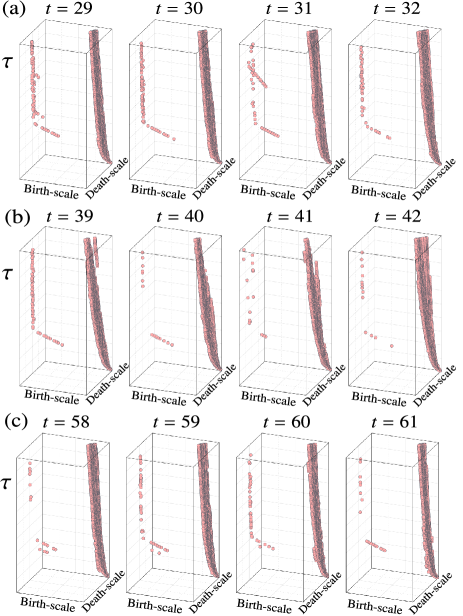
Figure 9: Three-dimensional persistence diagrams of one-dimensional holes for the Drosophila melanogaster gene regulatory networks spanning from (a) $t=29$ to $t=32$, (b) $t=39$ to $t=42$, and (c) $t=58$ to $t=61$. The birth-scale and the death-scale axes of the diagrams are represented at the logarithmic scale.

Figure 10: Kernel Fisher discriminant ratio $\kappa$ calculated from the three-dimensional persistence diagrams of one-dimensional holes for the time-evolving Drosophila melanogaster gene regulatory networks. Transition time points are detected in the sliding windows spanning between two different developmental stages. In each window, the transition time point $t_{c}$ is the time index of the maximum $\kappa$ value marked with the orange point of the dashed line. (a) Windows from the embryonic stage to the larval stage with time points $26\rightarrow 36$ ($t_{c}=28$), $27\rightarrow 37$ ($t_{c}=28$), and $28\rightarrow 38$ ($t_{c}=31$). (b) Windows from the larval stage to the pupal stage with time points $36\rightarrow 46$ ($t_{c}=41$), $37\rightarrow 47$ ($t_{c}=41$) and $38\rightarrow 48$ ($t_{c}=41$). (c) Windows from the pupal stage to the adulthood stage with time points $54\rightarrow 64$ ($t_{c}=59$), $55\rightarrow 65$ ($t_{c}=59$) and $56\rightarrow 66$ ($t_{c}=59$).

We apply the scale-variant topological features to detect transition points between the developmental stages of Drosophila melanogaster in the time-evolving gene regulatory networks. Particularly, we use a genome-wide microarray profiling, which shows the expression patterns of 4028 genes simultaneously measured during the developmental stages of Drosophila melanogaster Arbeitman et al. (2002). Herein, 66 time points are chosen from the full developmental cycle: embryonic stage (1–30), larval stage (31–40), pupal stage (41–58), and adulthood stage (59–66) Zhang and Cao (2017). We use kernel reweighted logistic regression method Song et al. (2009) to reconstruct the time-evolving networks for 588 genes, which are known to be related to the developmental process based on their gene ontologies. Therefore, the networks are reconstructed via logistic regression using only binary information, i.e., activation or non-activation of gene expression data. For the likelihood being maximized for network inference, a kernel weight function is employed to obtain the dynamic networks structures with smooth transition at adjacent time points Song et al. (2009).

We use the scale-variant topological features to detect the transition points with respect to the topological structure of the constructed time-evolving networks. Consequently, the detected transition points agree with the transition points in the dynamics of Drosophila melanogaster. Here, the change points between the developmental stages of Drosophila melanogaster chosen in the experiment are referred to as the transition points in the dynamics: $t_{1}=31$ between the embryonic stage and the larval stage, $t_{2}=41$ between the larval stage and the pupal stage, and $t_{3}=59$ between the pupal stage and the adulthood stage. For the network of each time point, three-dimensional persistence diagrams are computed for one-dimensional holes with $\tau_{1}=1,\ldots,\tau_{100}=100$. Figure 9 shows the examples of the diagrams for networks spanning from (a) $t=29$ to $t=32$, (b) $t=39$ to $t=42$, and (c) $t=58$ to $t=61$. Here, note the transformation of the patterns in scale-variant topological features along with time points. Such patterns transformation corresponds with the transformation in the topological structure of time-evolving reconstructed networks. Moreover, we quantify the transition points with respect to the topological structure by observing the sliding windows spanning two different developmental stages of Drosophila melanogaster. In each sliding window, we compute the kernel Fisher discriminant ratio Harchaoui et al. (2009) for each time point from the three-dimensional persistence diagrams of the networks (see Appendix D). The time point of the maximum ratio can be identified as the transition time point $t_{c}$ in each window (Fig. 10). From the embryonic stage to the larval stage, we obtain the transition time points in the topological structure as $t_{c}=28$ and $t_{c}=31$, relatively close to the experimentally known transition time point $t_{1}=31$. Furthermore, from the larval stage to the pupal stage, and from the pupal stage to the adulthood stage, we obtain the transition time points in the topological structure as $t_{c}=41$ and $t_{c}=59$, respectively. These points agree with the experimentally known transition time points $t_{2}=41$ and $t_{3}=59$.

III.5 Considerations on the maximum value of the diffusion timescale

We investigate the maximum timescale $\tau_{\textup{max}}$ to examine the length of the diffusion process must be explored. Note that the timescale functions as a resolution parameter to unravel the multi-scale and hierarchical structure of a network. A small timescale restricts random walkers in local interactions, which produces many communities in the network. In contrast, a large timescale leads to a substantial contribution of long walks and therefore yields a small number of communities because random walkers tend to remain in these communities for a long time. This resolution problem has been addressed in Refs. Delvenne et al. (2010); Lambiotte et al. (2014), in which the relevance of partitions as community structures is characterized over timescales. Instead of characterizing the network structure at a fixed resolution, the scale-variant topological features obtained with a sufficiently large $\tau_{\textup{max}}$ can contain information about the network at multiple resolutions.

Here, we study the method for determining $\tau_{\textup{max}}$ through the spectral decomposition of the normalized Laplacian of the network. Denoting the eigenvalues of $\bm{L}^{\text{rw}}_{\mathcal{G}}$ by $\lambda_{i}$ in increasing order $0=\lambda_{1}\leq\lambda_{2}\leq\ldots\leq\lambda_{n}$, the spectral decomposition of $\bm{L}^{\text{rw}}_{\mathcal{G}}$ is expressed as follows:

$$\bm{L}^{\text{rw}}_{\mathcal{G}}=\sum_{i=1}^{n}\lambda_{i}\bm{\theta}^{\top}_{i}\bm{\theta}_{i},$$ (7)

where $\bm{\theta}_{i}$ is the eigenvector associated with $\lambda_{i}$. Therefore, the solution for Eq. (1) can be written as follows:

$$\bm{p}_{\mathcal{G}}(\tau|i)=\sum_{i=1}^{n}\exp{(-\lambda_{i}\tau)}\bm{u}_{i}\bm{\theta}^{\top}_{i}\bm{\theta}_{i}.$$ (8)

From Eq. (8), each eigenvalue $\lambda_{i}$ of $\bm{L}^{\text{rw}}_{\mathcal{G}}$ is associated with a decaying mode in the diffusion process with the characteristic timescale $\tau=1/\lambda_{i}$. Therefore, if there are large gaps between eigenvalues, for example if the $k_{0}$ smallest eigenvalues $\{\lambda_{1}=0,\ldots,\lambda_{k_{0}}\}$ are greatly separated from the remaining eigenvalues ($\lambda_{k_{0}}\ll\lambda_{k_{0}+1}=\lambda_{\textup{sep}}$), we can ignore the terms associated with $\{\lambda_{k_{0}+1},\ldots,\lambda_{n}\}$ in Eq. (8) at $\tau$ satisfying $\tau\lambda_{\textup{sep}}\gg 1$. Thus, there is no significant change in the formation of clusters or loops in the mapped point cloud $P_{\mathcal{G}}(\tau)$, nor in the formation of communities in the network at the $\tau$-scale. Therefore, as a heuristic method, if we consider $\tau_{\textup{max}}$ such that $\tau_{\textup{max}}\lambda_{\textup{sep}}\gg 1$, the structure of the network is well characterized via the scale-variant topological features.

Here, we verify the above consideration by distinguishing the network of the Barabási–Albert (BA) growth model Barabási and Albert (1999) with its configuration network. The network is initialized with $m_{0}$ nodes and no edges. At each time step, each new node is added with no more than $m_{0}$ links to the existing nodes in the network. The probability that a new node is connected to an existing node is proportional to the degree of the existing node. Note that both the BA networks and their configuration networks have a scale-free property with degree exponent 3. We set the number of nodes to 128, vary the number of initial nodes $m_{0}=1,2,\ldots,50$, and generate 10 networks via this process for each value of $m_{0}$. The 10 networks generated at each $m_{0}$ are split into two parts, with five networks for training and the remaining five for testing. Figure 11 depicts eigenvalues $\lambda_{k}$ such that $0.0\leq\lambda_{k}\leq 0.5$ for (a) BA networks and (b) scale-free configuration networks. The colors of the points correspond to values of $m_{0}=1,2,3,4,5,6$. From Fig. 11, we can identify the value of $\lambda_{\textup{sep}}$ to separate the eigenvalues for each network. The smallest $\lambda_{\textup{sep}}$ values for BA networks and configuration networks are $\lambda^{\text{BA}}_{\textup{sep}}\approx 0.18$ and $\lambda^{\text{conf}}_{\textup{sep}}\approx 0.16$, respectively. Therefore, $\tau_{\textup{max}}$ should be set to $\tau_{\textup{max}}\lambda^{\text{BA}}_{\textup{sep}}\gg 1$ and $\tau_{\textup{max}}\lambda^{\text{conf}}_{\textup{sep}}\gg 1$, for instance, $\tau_{\textup{max}}\lambda^{\text{BA}}_{\textup{sep}}>10$ and $\tau_{\textup{max}}\lambda^{\text{conf}}_{\textup{sep}}>10$, or $\tau_{\textup{max}}\geq 65$.

For each $\tau_{\textup{max}}$ in $\{5,10,15,\ldots,95,100\}$, we compute three-dimensional persistence diagrams of one-dimensional holes with $\tau_{1}=1,\tau_{2}=2,\tau_{3}=3,\ldots,\tau_{K}=\tau_{\textup{max}}$. The line in Fig. 12 depicts the average test accuracy over 100 random train-test splits at each value of $\tau_{\textup{max}}$. The shaded area indicates the confidence intervals of one standard deviation calculated using the ensemble of runs. In general, increasing $\tau_{\textup{max}}$ serves to increase classification accuracy because the diffusion process gathers more information about the network structure. There is a transition in classification accuracy with large deviations when $\tau_{\textup{max}}$ increases from 30 to 40. To demonstrate this transition in more detail, we plot $\tau_{\textup{max}}=20,21,\ldots,49,50$ in the inset of Fig. 12. For $\tau_{\textup{max}}<30$, only microscale structures are considered in the features, which has a small effect on the differences between networks. The transition occurs when the mesoscale structures are considered. For $\tau_{\textup{max}}>40$, the deviation is reduced as the mesoscale structures are revealed. For sufficiently large $\tau_{\textup{max}}$ ($\tau_{\textup{max}}\geq 65$), the method achieves high accuracy in the range of 94$\%$ to 94.5$\%$. This observation agrees with the above-mentioned heuristic for determining $\tau_{\textup{max}}$.

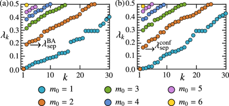
Figure 11: Eigenvalues $\lambda_{k}$ such that $0\leq\lambda_{k}\leq 0.5$ for (a) Barabási–Albert (BA) networks and (b) scale-free configuration networks. The colors of the points correspond to values of $m_{0}=1,2,3,4,5,6$ (number of initial nodes in the BA growth model). The value of $\lambda_{\textup{sep}}$ to effectively separate eigenvalues is identified for each network. The smallest $\lambda_{\textup{sep}}$ values for the BA networks and configuration networks are $\lambda^{\text{BA}}_{\textup{sep}}\approx 0.18$ and $\lambda^{\text{conf}}_{\textup{sep}}\approx 0.16$, respectively, as marked.

Figure 12: Classification of networks generated from Barabási–Albert models with their configuration networks using scale-variant topological features. The line depicts the average test accuracy over 100 random train-test splits at each value of $\tau_{\textup{max}}$. The shaded area indicates the confidence intervals of one standard deviation calculated using the same ensemble of runs. The inset highlights the transition in accuracy over $\tau_{\textup{max}}=20\text{--}50$.

IV Concluding remarks and discussion

Our study mainly aimed to represent the variation of topological scales, capture the nondyadic interactions, and provide robustness against noise in characterizing the structure of complex networks. Here, we proposed a general framework for constructing the scale-variant topological features from the diffusion process exhibited in networks. The scale-variant topological features do not directly correspond to the common statistical measures that are constructed from the dyadic interactions between nodes at a single fixed topological scale. Rather, our features encode the information of both dyadic and nondyadic interactions in networks at variant topological scales.

In the networks classification, our features acted as strong factors to identify the networks. Theoretically, we derived a strong mathematical guarantee for the robustness of these features with respect to the perturbations applied to the networks. Through several experiments, we provided an empirical evidence for the effectiveness of these features in applications, such as classification of real-world networks and detection of transition points, with respect to the topological structure in time-evolving networks. The results suggested that the observation of the topological features induced from the network dynamics over variant scales can characterize the structure and provide important insights for understanding the functionality of networks.

In our experiments, the scale-variant topological features were constructed from zero-dimensional and one-dimensional holes. In principle, we can compute the features from higher-dimensional holes that represent nondyadic interactions, involving a larger number of nodes in each interaction. However, to investigate the features from high-dimensional holes, the Vietoris–Rips filtration used in our study can consist of a large number of simplices. More precisely, to consider $l$-dimensional holes, the Vietoris–Rips filtration has size $O(N^{l+2})$ of the number of simplices. Herein, $N$ is the number of nodes in the network. This observation shows the difficulty of using the features from $l$-dimensional holes ($l\geq 2$) for networks with a large number of nodes. On the contrary and as demonstrated in this paper, we found it sufficient to use $l$-dimensional holes with $l=0,1$ in practical applications. Furthermore, one can replace the Vietoris–Rips filtration with the Witness filtration De Silva and Carlsson (2004) or the approximation of the Vietoris–Rips filtration Sheehy (2012) for more efficient computations. We employed recent algorithmic improvements to efficiently compute the persistent diagrams with the core implementation referenced from Ripser libary Bauer (2017).

Another point to discuss is the selection of the maximum diffusion timescale. In our experiments, our method was only tested for small and medium-sized networks with less than 5,000 nodes per network. For larger networks, a longer diffusion timescale must be explored. This consideration will increase the computational cost of computing persistence diagrams and the kernel. However, this limitation can be mitigated by increasing the sampling interval to take discrete values of the timescale while keeping the maximum timescale sufficiently large. It is also possible to study the process of taking values of timescales based on the spectral decomposition of the normalized Laplacian of the network.

Our study is motivated by Ref. De Domenico (2017), in which the diffusion geometry from the diffusion process is used to reveal functional clusters in a network. Based on random walk dynamics, the diffusion distance between a pair of nodes in a network is defined and averaged in a range of timescales to model the underlying geometry of the network. However, the variation in network structure over the diffusion timescale is not discussed. In Ref. Lambiotte et al. (2014), a random walk process corresponding to the natural dynamics of a system focuses on recovering dynamically meaningful communities in the network. Our approach involves a diffusion process similar to that mentioned in Refs. Lambiotte et al. (2014); De Domenico (2017); however, it mainly focuses on the systematic representation of networks via topological data analysis by tracking the variation of the topological structures along timescales of the diffusion process.

In general, our study presented a unified analysis of complex networks. This study paves several opportunities for designing effective algorithms in network science, such as an investigation of more complicated network structures. For instance, we can employ our framework to study different aspects of multiplex networks, or to study the structural reducibility of a multilayer network while preserving its dynamics and function.

V Acknowledgments

This work was supported by Ministry of Education, Culture, Sports, Science and Technology (MEXT) KAKENHI Grants No. JP16K00325 and No. JP19K12153.

Appendix A Construction of Vietoris–Rips filtration of a network

We define and describe in Fig. 13 the process of extracting topological features of a complex network at each specific timescale $\tau$. At each $\tau$, we calculate the diffusion distance matrix $\bm{\Delta}_{\tau}$ of size $N\times N$, whose element $\Delta_{ij}$ is the Euclidean distance between points $\bm{p}_{\mathcal{G}}(\tau|i)$ and $\bm{p}_{\mathcal{G}}(\tau|j)$ [Fig. 13(a)]. If $\varepsilon=0$, the nodes of the network can be considered discrete points. As we increase $\varepsilon$, new pairwise connections and simplices may appear when $\varepsilon$ meets each value of $\Delta_{ij}$. We obtain a filtration as a sequence of embedded simplicial complexes. Hole patterns such as connected components (zero-dimensional holes) or loops (one-dimensional holes) can appear or disappear over this filtration. For instance, in Fig. 13(b), at $\varepsilon=0$, we have six separated nodes considered as six separated connected components, but at $\varepsilon=0.407$, three nodes are connected with each other; thus, two connected components disappear at this scale. We can describe these patterns as two blue bars started at scale $0$ and ended at scale $0.407$. The same explanation with the red bar started at scale $0.428$ and ended at scale $0.430$, which represents the emergence of loop pattern ($v_{1}\rightarrow v_{2}\rightarrow v_{3}\rightarrow v_{5}\rightarrow v_{1}$) at $\varepsilon=0.428$ and the disappearance at $\varepsilon=0.430$. Figure 13(c) illustrates the corresponding persistence diagrams for zero-dimensional holes and one-dimensional holes, where the birth-scale and the death-scale are represented for the values of $\varepsilon$ at the emergence and the disappearance of the holes.

Figure 13: An exemplary of Vietoris–Rips filtration constructed from a complex network $\mathcal{G}$ at a specific timescale $\tau$ ($\tau=1$ in this example). We map nodes $v_{1},\ldots,v_{N}$ of the network $\mathcal{G}$ to a point cloud of $N$ points $\bm{p}_{\mathcal{G}}(\tau|1),\ldots,\bm{p}_{\mathcal{G}}(\tau|N)$ through a diffusion dynamics described by the random walk Laplacian $\bm{L}^{\text{rw}}_{\mathcal{G}}$. (a) Diffusion distance matrix $\bm{\Delta}_{\tau}$ of size $N\times N$, whose element $\Delta_{ij}$ is the Euclidean distance between points $\bm{p}_{\mathcal{G}}(\tau|i)$ and $\bm{p}_{\mathcal{G}}(\tau|j)$. (b) A complex is built over a set of points if the pairwise distances between them are less than or equal to a threshold parameter $\varepsilon$. If $\varepsilon=0$, we have the discrete points. As $\varepsilon$ takes the increasing sequence values of diffusion distance $\Delta_{ij}$, the hole patterns such as connected components (zero-dimensional hole) or loops (one-dimensional hole) can appear or disappear over this filtration. The lifetime of these hole patterns are described as blue bars (for zero-dimensional holes) and red bars (for one-dimensional holes). These bars begin at the values of $\varepsilon$ when the holes appear, then end at values when the holes disappear. (c) The corresponding persistence diagrams for zero-dimensional and one-dimensional holes. The birth-scale and the death-scale are represented for the values of $\varepsilon$ at the emergence and the disappearance of the holes.

Appendix B Proof of the stability of the scale-variant topological features

We prove the result in Eq. (4). First, we introduce the concept of the bottleneck distance between two two-dimensional diagrams. Let $X$ and $Y$ be finite sets of points embedded in the Euclidean space $\mathbb{R}^{n}$. Denote their $two$-dimensional persistence diagrams for $l$-dimensional holes as $\mathcal{S}_{(l)}^{(2)}(X)$ and $\mathcal{S}_{(l)}^{(2)}(Y)$, respectively. We consider all matchings, $\gamma$, such that a point on one diagram is matched to a point on the other diagram or to its projection on the line $b=d$ in two-dimensional space. The bottleneck distance $d^{(2)}_{\textup{B}}$ between $\mathcal{S}_{(l)}^{(2)}(X)$ and $\mathcal{S}_{(l)}^{(2)}(Y)$ is defined as the infimum of the longest matched infinity-norm distance over all matchings, $\gamma$:

$$d^{(2)}_{\textup{B}}(\mathcal{S}_{(l)}^{(2)}(X),\mathcal{S}_{(l)}^{(2)}(Y))=\inf_{\gamma}\max_{(\bm{q}^{(1)},\bm{q}^{(2)})\in\gamma}\|\bm{q}^{(1)}-\bm{q}^{(2)}\|_{\infty}.$$ (9)

Here, $\|\bm{q}^{(1)}-\bm{q}^{(2)}\|_{\infty}=\max\left(|b_{1}-b_{2}|,|d_{1}-d_{2}|\right)$ for which $\bm{q}^{(1)}=(b_{1},d_{1})$ and $\bm{q}^{(2)}=(b_{2},d_{2})$.

The bottleneck distance between the two-dimensional persistence diagrams satisfies the following inequality Chazal et al. (2014):

$$d^{(2)}_{\textup{B}}(\mathcal{S}_{(l)}^{(2)}(X),\mathcal{S}_{(l)}^{(2)}(Y))\leq 2d_{\textup{H}}(X,Y),$$ (10)

where $d_{\textup{H}}(X,Y)$ is the Hausdorff distance given as

$$d_{\textup{H}}(X,Y)=\max\left\{\max_{\bm{x}\in X}\min_{\bm{y}\in Y}d(\bm{x},\bm{y}),\max_{\bm{y}\in Y}\min_{\bm{x}\in X}d(\bm{x},\bm{y})\right\}.$$ (11)

Here, $d(\bm{x},\bm{y})$ is the Euclidean distance between two points $\bm{x},\bm{y}$ in $\mathbb{R}^{n}$.

Given two three-dimensional persistence diagrams as $E$ and $F$, consider all matchings $\psi$ such that a point on one diagram is matched to a point on the other diagram or to its projection on the plane $b=d$. For each pair $(\bm{q}^{(1)},\bm{q}^{(2)})\in\psi$ for which $\bm{q}^{(1)}=\left(b_{1},d_{1},\tau_{1}\right)$ and $\bm{q}^{(2)}=\left(b_{2},d_{2},\tau_{2}\right)$, we define the relative infinity-norm distance between $\bm{q}^{(1)}$ and $\bm{q}^{(2)}$ as $d^{(\infty)}_{\xi}(\bm{q}^{(1)},\bm{q}^{(2)})=\max\left(|b_{1}-b_{2}|,|d_{1}-d_{2}|,\xi|\tau_{1}-\tau_{2}|\right)$, where $\xi$ is a positive rescaling coefficient introduced to adjust the scale difference between the point-wise distance and time. The bottleneck distance, $d^{(3)}_{\textup{B},\xi}(E,F)$, is defined as the infimum of the longest matched relative infinity-norm distance over all matchings $\psi$:

$$d^{(3)}_{\textup{B},\xi}(E,F)=\inf_{\psi}\max_{(\bm{q}^{(1)},\bm{q}^{(2)})\in\psi}d^{(\infty)}_{\xi}(\bm{q}^{(1)},\bm{q}^{(2)}).$$ (12)

For each $\tau\in\mathcal{T}$ and two networks $\mathcal{G},\mathcal{H}$ with the same number $N$ of nodes, we first prove the following inequality:

$$d^{(2)}_{\textup{B}}(D_{(l),\tau}^{(2)}(\mathcal{G}),D_{(l),\tau}^{(2)}(\mathcal{H}))\leq 2\tau\|\bm{L}^{\text{rw}}_{\mathcal{G}}-\bm{L}^{\text{rw}}_{\mathcal{H}}\|_{2}.$$ (13)

Here, two two-dimensional persistence diagrams $D^{(2)}_{l,\tau}(\mathcal{G})$ and $D^{(2)}_{l,\tau}(\mathcal{H})$ are calculated for $l$-dimensional holes from two point clouds $P_{\mathcal{G}}(\tau)=\{\bm{p}_{\mathcal{G}}(\tau|1),\ldots,\bm{p}_{\mathcal{G}}(\tau|N)\}$ and $P_{\mathcal{H}}(\tau)=\{\bm{p}_{\mathcal{H}}(\tau|1),\ldots,\bm{p}_{\mathcal{H}}(\tau|N)\}$, respectively.

Since $D_{(l),\tau}^{(2)}(\mathcal{G})=\mathcal{S}_{(l)}(P_{\mathcal{G}}(\tau))$ and $D_{(l),\tau}^{(2)}(\mathcal{H})=\mathcal{S}_{(l)}(P_{\mathcal{H}}(\tau))$, we apply Eq. (10) to have

$$d^{(2)}_{\textup{B}}(D_{(l),\tau}^{(2)}(\mathcal{G}),D_{(l),\tau}^{(2)}(\mathcal{H})) =d^{(2)}_{\textup{B}}(\mathcal{S}_{(l)}(P_{\mathcal{G}}(\tau)),\mathcal{S}_{(l)}(P_{\mathcal{H}}(\tau)))$$

$$\leq 2d_{\textup{H}}(P_{\mathcal{G}}(\tau),P_{\mathcal{H}}(\tau)).$$ (14)

From the definition of the Hausdorff distance, we have

$$d_{\textup{H}}(P_{\mathcal{G}}(\tau),P_{\mathcal{H}}(\tau)) =\max\left\{\max_{i}\min_{j}d(\bm{p}_{\mathcal{G}}(\tau|i),\bm{p}_{\mathcal{H}}(\tau|j)),\max_{j}\min_{i}d(\bm{p}_{\mathcal{G}}(\tau|i),\bm{p}_{\mathcal{H}}(\tau|j)))\right\}$$ (15)

$$\leq\max\left\{\max_{i}d(\bm{p}_{\mathcal{G}}(\tau|i),\bm{p}_{\mathcal{H}}(\tau|i)),\max_{j}d(\bm{p}_{\mathcal{G}}(\tau|j),\bm{p}_{\mathcal{H}}(\tau|j))\right\}=\max_{i}d(\bm{p}_{\mathcal{G}}(\tau|i),\bm{p}_{\mathcal{H}}(\tau|i)).$$ (16)

Since $\bm{p}_{\mathcal{G}}(\tau|i)=\bm{u}_{i}\exp(-\tau\bm{L}^{\text{rw}}_{\mathcal{G}})$ and $\bm{p}_{\mathcal{H}}(\tau|i)=\bm{u}_{i}\exp(-\tau\bm{L}^{\text{rw}}_{\mathcal{H}})$, we have

$$d(\bm{p}_{\mathcal{G}}(\tau|i),\bm{p}_{\mathcal{H}}(\tau|i)) =\|\bm{u}_{i}(e^{-\tau\bm{L}^{\text{rw}}_{\mathcal{G}}}-e^{-\tau\bm{L}^{\text{rw}}_{\mathcal{H}}})\|_{2}$$ (17)

$$\leq\|\bm{u}_{i}\|_{2}\|e^{-\tau\bm{L}^{\text{rw}}_{\mathcal{G}}}-e^{-\tau\bm{L}^{\text{rw}}_{\mathcal{H}}}\|_{2}$$ (18)

$$=\|e^{-\tau\bm{L}^{\text{rw}}_{\mathcal{G}}}-e^{-\tau\bm{L}^{\text{rw}}_{\mathcal{H}}}\|_{2}.$$ (19)

We write the difference of the matrix exponential in terms of an integral Golub and Van Loan (2012),

$$\|e^{-\tau\bm{L}^{\text{rw}}_{\mathcal{G}}}-e^{-\tau\bm{L}^{\text{rw}}_{\mathcal{H}}}\|_{2} =\bigg{\|}\int_{0}^{\tau}e^{-\bm{L}^{\text{rw}}_{\mathcal{G}}(\tau-t)}\bm{E}e^{-\bm{L}^{\text{rw}}_{\mathcal{H}}t}dt\bigg{\|}_{2}$$ (20)

$$\leq\int_{0}^{\tau}\|e^{-\bm{L}^{\text{rw}}_{\mathcal{G}}(\tau-t)}\bm{E}e^{-\bm{L}^{\text{rw}}_{\mathcal{H}}t}\|_{2}dt$$ (21)

$$\leq\|\bm{E}\|_{2}\int_{0}^{\tau}\|e^{-\bm{L}^{\text{rw}}_{\mathcal{G}}(\tau-t)}\|_{2}\|e^{-\bm{L}^{\text{rw}}_{\mathcal{H}}t}\|_{2}dt,$$ (22)

where $\bm{E}=\bm{L}^{\text{rw}}_{\mathcal{G}}-\bm{L}^{\text{rw}}_{\mathcal{H}}$. We know that $-\bm{L}^{\text{rw}}_{\mathcal{G}}$ is a negative semi-definite matrix with the largest eigenvalue equal to 0. It implies that the largest eigenvalue of $e^{-\bm{L}^{\text{rw}}_{\mathcal{G}}(\tau-t)}$ is equal to 1, and hence $\|e^{-\bm{L}^{\text{rw}}_{\mathcal{G}}(\tau-t)}\|_{2}=1$. We obtain the same result with $-\bm{L}^{\text{rw}}_{\mathcal{H}}$, i.e., $\|e^{-\bm{L}^{\text{rw}}_{\mathcal{H}}t}\|_{2}=1$. Then, from Eq. (19) and Eq. (22), we have

$$d(\bm{p}_{\mathcal{G}}(\tau|i),\bm{p}_{\mathcal{H}}(\tau|i)) \leq\|\bm{E}\|_{2}\int_{0}^{\tau}1dt$$ (23)

$$=\tau\|\bm{E}\|_{2}=\tau\|\bm{L}^{\text{rw}}_{\mathcal{G}}-\bm{L}^{\text{rw}}_{\mathcal{H}}\|_{2}.$$ (24)

From Eq. (14), Eq. (16) and Eq. (24), we have the result in Eq. (13).

Let $\Gamma_{\tau}$ be the set of matchings defined in Eq. (9) between two two-dimensional persistence diagrams $D_{(l),\tau}^{(2)}(\mathcal{G})$ and $D_{(l),\tau}^{(2)}(\mathcal{H})$. For each collection $\Lambda=\{\gamma_{1},\gamma_{2},\ldots,\gamma_{K}\mid\gamma_{i}\in\Gamma_{\tau_{i}},i=1,2,\ldots,K\}$, we construct the matching $\psi$ between two three-dimensional persistence diagrams $D_{(l)}^{(3)}(\mathcal{G})$ and $D_{(l)}^{(3)}(\mathcal{H})$, such that, for each $(\bm{q}^{(1)},\bm{q}^{(2)})\in\psi$, then $\bm{q}^{(1)}=(b_{1},d_{1},\tau)$, $\bm{q}^{(2)}=(b_{2},d_{2},\tau)$, and $(\bm{q}^{(1)}_{\gamma},\bm{q}^{(2)}_{\gamma})\in\gamma$, where $\bm{q}^{(1)}_{\gamma}=(b_{1},d_{1})$, $\bm{q}^{(2)}_{\gamma}=(b_{2},d_{2})$ and $\gamma\in\Lambda\cap\Gamma_{\tau}$. Let $\Gamma$ be a set of all matchings $\psi$ constructed this way. From the definition of the bottleneck distance, we have the following inequality:

$$d^{(3)}_{\textup{B},\xi}(D_{(l)}^{(3)}(\mathcal{G}),D_{(l)}^{(3)}(\mathcal{H}))\leq\inf_{\psi\in\Gamma}\max_{(\bm{q}^{(1)},\bm{q}^{(2)})\in\psi}d^{(\infty)}_{\xi}(\bm{q}^{(1)},\bm{q}^{(2)}).$$ (25)

For $(\bm{q}^{(1)},\bm{q}^{(2)})\in\psi$, we have

$$d^{(\infty)}_{\xi}(\bm{q}^{(1)},\bm{q}^{(2)}) =\max\{|b_{1}-b_{2}|,|d_{1}-d_{2}|,\xi|\tau-\tau|\}$$ (26)

$$=\max\{|b_{1}-b_{2}|,|d_{1}-d_{2}|\}$$ (27)

$$=\|\bm{q}^{(1)}_{\gamma}-\bm{q}^{(2)}_{\gamma}\|_{\infty},$$ (28)

and Eq. (25) becomes

$$d^{(3)}_{\textup{B},\xi}(D_{(l)}^{(3)}(\mathcal{G}),D_{(l)}^{(3)}(\mathcal{H})) \leq\max_{\tau\in\mathcal{T}}\inf_{\gamma\in\Gamma_{\tau}}\max_{(\bm{q}^{(1)}_{\gamma},\bm{q}^{(2)}_{\gamma})\in\gamma}\|\bm{q}^{(1)}_{\gamma}-\bm{q}^{(2)}_{\gamma}\|_{\infty}$$ (29)

$$=\max_{\tau\in\mathcal{T}}d^{(2)}_{\textup{B}}(D_{(l),\tau}^{(2)}(\mathcal{G}),D_{(l),\tau}^{(2)}(\mathcal{H})).$$ (30)

From Eq. (13) and Eq. (30), we obtain Eq. (4) in the main text, which is the stability property of our scale-variant features.

Appendix C Selecting parameters for the kernel

In the kernel $\mathcal{K}_{\sigma,\xi}$ defined in Eq. (5), we set the rescale coefficient to $\xi=\sigma$ and present here a heuristic method to select the bandwidth $\sigma$. Given the kernel values calculated from the three-dimensional persistence diagrams $D_{(l),1}^{(3)},D_{(l),2}^{(3)},\ldots,D_{(l),M}^{(3)}$ of $l$-dimensional holes, we denote $\sigma^{2}_{s}=\text{median}\{(b_{i}-b_{j})^{2}+(d_{i}-d_{j})^{2}\mid(b_{i},d_{i},\tau_{i}),(b_{j},d_{j},\tau_{j})\in D_{(l),s}^{(3)}\}$ with $s=1,2,\ldots,M$. We set $\sigma$ as $\sigma^{2}=\dfrac{1}{2}\text{median}\{\sigma^{2}_{s}\mid s=1,\ldots,M\}$ such that $2\sigma^{2}$ takes values close to many $(b_{i}-b_{j})^{2}+(d_{i}-d_{j})^{2}$ values.

Appendix D Kernel Fisher discriminant ratio

Consider a collection of three-dimensional diagrams $\mathcal{D}_{(l)}=\{D_{(l),1}^{(3)},D_{(l),2}^{(3)},\ldots,D_{(l),M}^{(3)}\}$ of $l$-dimensional holes. Since $\mathcal{K}_{\sigma,\xi}$ is a positive-definite kernel on $\mathcal{D}_{(l)}$ Tran and Hasegawa (2019), there exists a Hilbert space $H_{b}$ and a mapping $\Phi:\mathcal{D}_{(l)}\longrightarrow H_{b}$ such that for $E\in\mathcal{D}_{(l)}$, $\Phi$ maps $E$ to a function $\Phi_{E}\in H_{b}$ that satisfies

$$\forall E,F\in\mathcal{D}_{(l)},\mathcal{K}_{\sigma,\xi}(E,F)=\langle\Phi_{E},\Phi_{F}\rangle_{H_{b}}.$$ (31)

Here, $H_{b}$ is a real inner product space of function $f:\mathcal{D}_{(l)}\longrightarrow\mathbb{R}$, and thus, is a complete metric space with respect to the distance induced by the inner product $\langle\cdot,\cdot\rangle_{H_{b}}$.

Given an index $s>1$, the kernel Fisher discriminant ratio $\kappa_{M,s}(\mathcal{D}_{(l)})$ is a statistical quantity to measure the dissimilarity between two classes assumptively defined by two sets of diagrams having index before and from $s$ Harchaoui et al. (2009). The corresponding empirical mean and covariance functions in $H_{b}$ associated with the data in $\mathcal{D}_{(l)}$ having index before and from $s$ are defined as

$$\hat{\mu}_{1} =\dfrac{1}{s-1}\sum_{i=1}^{s-1}\Phi_{D_{(l),i}^{(3)}},$$ (32)

$$\hat{\Sigma}_{1} =\dfrac{1}{s-1}\sum_{i=1}^{s-1}\left\{\Phi_{D_{(l),i}^{(3)}}-\hat{\mu}_{1}\right\}\otimes\left\{\Phi_{D_{(l),i}^{(3)}}-\hat{\mu}_{1}\right\},$$ (33)

$$\hat{\mu}_{2} =\dfrac{1}{M-s+1}\sum_{i=s}^{M}\Phi_{D_{(l),i}^{(3)}},$$ (34)

$$\hat{\Sigma}_{2} =\dfrac{1}{M-s+1}\sum_{i=s}^{M}\left\{\Phi_{D_{(l),i}^{(3)}}-\hat{\mu}_{2}\right\}\otimes\left\{\Phi_{D_{(l),i}^{(3)}}-\hat{\mu}_{2}\right\}.$$ (35)

Here, $f\otimes g$ for two functions $f,g\in H_{b}$ is defined for all functions $h\in H_{b}$ as $(f\otimes g)h=\left<g,h\right>_{H_{b}}f$.

The kernel Fisher discriminant ratio $\kappa_{M,s}(\mathcal{D}_{(l)})$ is defined as

$$\kappa_{M,s}(\mathcal{D}_{(l)})$$

$$=\dfrac{(s-1)(M-s+1)}{M}\left<\hat{\mu}_{2}-\hat{\mu}_{1},(\hat{\Sigma}+\eta\bm{I})^{-1}(\hat{\mu}_{2}-\hat{\mu}_{1})\right>_{H_{b}},$$ (36)

where $\eta$ is a regularization parameter and $\hat{\Sigma}=\dfrac{s-1}{M}\hat{\Sigma}_{1}+\dfrac{M-s+1}{M}\hat{\Sigma}_{2}$. Here, the index $s$ achieving the maximum of $\kappa_{M,s}(\mathcal{D}_{(l)})$ corresponds to the estimated transition point.

We set $\eta=10^{-1},10^{-1},10^{-5}$ in the experiments of the Girvan–Newman (GN) network, Lancichinetti–Fortunato–Radicchi (LFR) network and Drosophila melanogaster network, respectively.

Appendix E Common measures for a network

For each network, we calculate the following 18 common measures: the density (the ratio of the existing to the possible edges), the transitivity Costa et al. (2007) (the proportion of triangles), the diameter (the maximum eccentricity), the radius (the minimum eccentricity), the degree assortativity coefficient Newman (2002), the global efficiency Latora and Marchiori (2001), the number of connected parts, the average clustering coefficient, the average number of triangles that include a node as a vertex, the average local efficiency Latora and Marchiori (2001), the average edge betweenness centrality Brandes (2008), the average node betweenness centrality Freeman (1978), the average node closeness centrality Freeman (1978), the average eccentricity, the average shortest paths, the average degree centrality Freeman (1978), the maximum modularity which is obtained by Louvain heuristic Blondel et al. (2008); Newman and Girvan (2004), and the average of global mean first-passage times of random walks on the network Tejedor et al. (2009). We normalize the measures in the range of $[0,1]$ using the min-max normalization (i.e. $f_{*}=(f_{*}-f_{\text{min}})/(f_{\text{max}}-f_{\text{min}})$, where $f_{\text{min}},f_{\text{max}}$ are the minimum and the maximum values of a measure in the data).

Appendix F Graph kernel methods

We describe the graph kernel methods used in the main text. The implementations of these graph kernels can be found in Ref. Sugiyama et al. (2017).

F.1 Random walk kernels

The random walk graph kernels measure the similarity between a pair of graphs based on the number of equal-length walks in two graphs. Given two unlabeled graphs $\mathcal{G}$ and $\mathcal{G}^{\prime}$ with their vertex and edge sets as $(\mathcal{V},\mathcal{E})$ and $(\mathcal{V}^{\prime},\mathcal{E}^{\prime})$, respectively, the direct product graph $\mathcal{G}_{\times}=(\mathcal{V}_{\times},\mathcal{E}_{\times})$ of $\mathcal{G}$ and $\mathcal{G}^{\prime}$ is a graph with the node set $\mathcal{V}_{\times}=\{(v,v^{\prime})\mid v\in\mathcal{V},v^{\prime}\in\mathcal{V}^{\prime}\}$ and the edge set $\mathcal{E}_{\times}=\{((v_{a},v^{\prime}_{a}),(v_{b},v^{\prime}_{b}))\mid(v_{a},v_{b})\in\mathcal{E},(v^{\prime}_{a},v^{\prime}_{b})\in\mathcal{E}^{\prime}\}$.

The KStepRW kernel is the $k$-step random walk kernel $\mathcal{K}_{\times}^{k}$ defined as

$$\mathcal{K}_{\times}^{k}(\mathcal{G},\mathcal{G}^{\prime})=\sum_{i,j=1}^{|\mathcal{V}_{\times}|}\sum_{m=0}^{k}\left[\lambda_{m}\bm{W}_{\times}^{m}\right]_{ij},$$ (37)

where $\bm{W}_{\times}$ is a weight matrix of $\mathcal{G}_{\times}$ and $\lambda_{0},\ldots,\lambda_{k}$ is a sequence of positive, real-valued weights. In our experiments, we set $k=2$ and $\lambda_{0}=\lambda_{1}=\lambda_{2}=1.0$.

GeometricRW kernel is a specific case of the $k$-step random walk kernel, when $k$ goes to infinity and the weights are the geometric series, i.e., $\lambda_{m}=\lambda^{m}$ ($\lambda=0.05$ in our experiments). The GeometricRW kernel is defined as

$$\mathcal{K}_{\text{GR}}(\mathcal{G},\mathcal{G}^{\prime})=\sum_{i,j=1}^{|\mathcal{V}_{\times}|}\sum_{m=0}^{\infty}\left[\lambda^{m}\bm{W}_{\times}^{m}\right]_{ij}=\sum_{i,j=1}^{|V_{\times}|}\left[(\bm{I}-\lambda\bm{W}_{\times})^{-1}\right],$$ (38)

where $\bm{I}$ is an identity matrix of size $|\mathcal{V}_{\times}|\times|\mathcal{V}_{\times}|$.

ExponentialRW kernel is a specific case of the $k$-step random walk kernel, when $k$ goes to infinity and the weights are the exponential series, i.e., $\lambda_{m}=\frac{\beta^{m}}{m!}$ ($\beta=0.1$ in our experiments). The ExponentialRW kernel is defined as

$$\mathcal{K}_{\text{EX}}(\mathcal{G},\mathcal{G}^{\prime})=\sum_{i,j=1}^{|V_{\times}|}\sum_{m=0}^{\infty}\left[\dfrac{(\beta\bm{W}_{\times})^{m}}{m!}\right]_{ij}=\sum_{i,j=1}^{|V_{\times}|}\left[e^{\beta\bm{W}_{\times}}\right]_{ij}.$$ (39)

F.2 ShortestPath kernel

ShortestPath kernel compares all pairs of the shortest path lengths from $\mathcal{G}$ and $\mathcal{G}^{\prime}$ defined as

$$\mathcal{K}_{\text{SP}}(\mathcal{G},\mathcal{G}^{\prime})=\sum_{v_{i},v_{j}\in\mathcal{G}}\sum_{v^{\prime}_{k},v^{\prime}_{l}\in\mathcal{G}^{\prime}}\delta(d(v_{i},v_{j}),d(v^{\prime}_{k},v^{\prime}_{l})),$$ (40)

where $d(v_{i},v_{j})$ and $d(v^{\prime}_{k},v^{\prime}_{l})$ are the lengths of the shortest path between nodes $v_{i}$ and $v_{j}$ in $\mathcal{G}$, and the shortest path between nodes $v^{\prime}_{k}$ and $v^{\prime}_{l}$ in $\mathcal{G}^{\prime}$, respectively. Here, $\delta(x,y)=1$ if $x=y$, and $0$ if $x\neq y$.

F.3 Graphlet kernel

A size-$k$ graphlet is an induced and non-isomorphic sub-graph of size $k$. Let $\mathcal{S}_{k}=\{G_{1},\ldots,G_{N_{k}}\}$ be a set of size-$k$ graphlets, where $N_{k}$ denotes the number of unique graphlets of size $k$. For an unlabeled graph $\mathcal{G}$ (the graph does not contain attributes for nodes), we define a vector $\bm{f}_{\mathcal{G}}$ of length $N_{k}$ such that the $i^{th}$ component of $\bm{f}_{\mathcal{G}}$ denotes the frequency of graphlet $G_{i}$ appearing as a subgraph of $\mathcal{G}$. Given two unlabeled graphs $\mathcal{G}$ and $\mathcal{G}^{\prime}$, the graphlet kernel is defined as

$$\mathcal{K}_{\text{GK}}(\mathcal{G},\mathcal{G}^{\prime})=\langle\bm{f}_{\mathcal{G}},\bm{f}_{\mathcal{G}^{\prime}}\rangle,$$ (41)

where $\langle\cdot,\cdot\rangle$ represents the Euclidean dot product. We set $k=4$ for MUTAG, BZR, DHFR and FRANKENSTEIN datasets and $k=3$ for the other datasets.

F.4 Weisfeiler–Lehman kernel

Weisfeiler–Lehman kernel decomposes a graph into its subtree patterns and compares these patterns in two graphs. For an unlabeled graph $\mathcal{G}$, all vertexes $v$ of $\mathcal{G}$ are initialized with label $\varphi(v)=0$. We iterate over each vertex $v$ and its neighbour to create a multiset label as $\varphi^{(i)}(v)$ such that $\varphi^{(1)}(v)=\varphi(v)$, and $\varphi^{(i)}$ with $i>1$ is defined as $\varphi^{(i)}(v)=(\varphi^{(i)}(v),\text{Q}^{(i-1)}_{v})$, where $\text{Q}^{(i-1)}_{v}$ is the sorted labels of $v$’s neighbours. To measure the similarity between graphs, we count the co-occurrences of the labels in both graphs for $h$ iterations with the kernel defined as

$$\mathcal{K}_{\text{WL}}(\mathcal{G},\mathcal{G}^{\prime})=\langle\bm{1}_{\mathcal{G}},\bm{1}_{\mathcal{G}^{\prime}}\rangle.$$ (42)

Here, $\bm{1}_{\mathcal{G}}$ is the vector concatenation of $h$ vertex label histograms $\bm{1}^{(1)}_{\mathcal{G}},\ldots,\bm{1}^{(h)}_{\mathcal{G}}$ in $h$ iterations. We set $h=5$ in our experiments.

References

- Taylor et al. (2015) D. Taylor, F. Klimm, H. A. Harrington, M. Kramár, K. Mischaikow, M. A. Porter, and P. J. Mucha, Nat. Commun. 6, 7723 (2015).
- Zañudo et al. (2017) J. G. T. Zañudo, G. Yang, and R. Albert, Proc. Natl. Acad. Sci. USA 114, 7234 (2017).
- Santolini and Barabási (2018) M. Santolini and A.-L. Barabási, Proc. Natl. Acad. Sci. USA 115, E6375 (2018).
- Sun et al. (2014) K. Sun, J. P. Gonçalves, C. Larminie, and N. Pržulj, BMC Bioinformatics 15, 304 (2014).
- Calderone et al. (2016) A. Calderone, M. Formenti, F. Aprea, M. Papa, L. Alberghina, A. M. Colangelo, and P. Bertolazzi, BMC Syst. Biol. 10, 25 (2016).
- Schieber et al. (2017) T. A. Schieber, L. Carpi, A. Díaz-Guilera, P. M. Pardalos, C. Masoller, and M. G. Ravetti, Nat. Commun. 8, 13928 (2017).
- Carpi et al. (2012) L. Carpi, P. Saco, O. Rosso, and M. Ravetti, Eur. Phys. J. B 85, 389 (2012).
- Barnett and Onnela (2016) I. Barnett and J.-P. Onnela, Sci. Rep. 6, 18893 (2016).
- Bao and Michailidis (2018) W. Bao and G. Michailidis, Sci. Rep. 8, 12938 (2018).
- Ahn et al. (2010) Y.-Y. Ahn, J. P. Bagrow, and S. Lehmann, Nature 466, 761 (2010).
- Betzel and Bassett (2017) R. F. Betzel and D. S. Bassett, Neuroimage 160, 73 (2017).
- Boulos et al. (2017) R. E. Boulos, N. Tremblay, A. Arneodo, P. Borgnat, and B. Audit, BMC Bioinformatics 18, 209 (2017).
- Costa et al. (2007) L. d. F. Costa, F. A. Rodrigues, G. Travieso, and P. R. Villas Boas, Adv. Phys. 56, 167 (2007).
- Newman (2010) M. E. J. Newman, Networks: An Introduction (Oxford Univ. Press, New York, NY, USA, 2010).
- Arenas et al. (2006) A. Arenas, A. Díaz-Guilera, and C. J. Pérez-Vicente, Phys. Rev. Lett. 96, 114102 (2006).
- Sales-Pardo et al. (2007) M. Sales-Pardo, R. Guimera, A. A. Moreira, and L. A. N. Amaral, Proc. Natl. Acad. Sci. USA 104, 15224 (2007).
- Lancichinetti et al. (2009) A. Lancichinetti, S. Fortunato, and J. Kertész, New J. Phys. 11, 033015 (2009).
- Tremblay and Borgnat (2014) N. Tremblay and P. Borgnat, IEEE Trans. Signal Process. 62, 5227 (2014).
- Marvel et al. (2011) S. A. Marvel, J. Kleinberg, R. D. Kleinberg, and S. H. Strogatz, Proc. Natl. Acad. Sci. USA 108, 1771 (2011).
- van der Schaft et al. (2013) A. van der Schaft, S. Rao, and B. Jayawardhana, SIAM J. Appl. Math. 73, 953 (2013).
- Reimann et al. (2017) M. W. Reimann, M. Nolte, M. Scolamiero, K. Turner, R. Perin, G. Chindemi, P. Dłotko, R. Levi, K. Hess, and H. Markram, Front. Comput. Neurosci. 11, 48 (2017).
- de Menezes and Barabási (2004) M. A. de Menezes and A.-L. Barabási, Phys. Rev. Lett. 92, 028701 (2004).
- Barabási et al. (2016) A.-L. Barabási et al., Network science (Cambridge Univ. Press, Cambridge, 2016).
- Broido and Clauset (2019) A. D. Broido and A. Clauset, Nat. Commun. 10, 1017 (2019).
- Carlsson (2009) G. Carlsson, Bull. Amer. Math. Soc. 46, 255 (2009).
- De Domenico (2017) M. De Domenico, Phys. Rev. Lett. 118, 168301 (2017).
- Edelsbrunner et al. (2002) H. Edelsbrunner, D. Letscher, and A. Zomorodian, Discrete Comput. Geom. 28, 511 (2002).
- Zomorodian and Carlsson (2005) A. Zomorodian and G. Carlsson, Discrete Comput. Geom. 33, 249 (2005).
- Edelsbrunner and Harer (2010) H. Edelsbrunner and J. Harer, Computational Topology. An Introduction (American Mathematical Society, Providence, RI, 2010).
- Kaczynski et al. (2006) T. Kaczynski, K. Mischaikow, and M. Mrozek, Computational homology, Vol. 157 (Springer, 2006).
- Tran and Hasegawa (2019) Q. H. Tran and Y. Hasegawa, Phys. Rev. E 99, 032209 (2019).
- Golub and Van Loan (2012) G. H. Golub and C. F. Van Loan, Matrix computations, 4th ed. (JHU Press, Baltimore, MD, USA, 2012).
- Chazal et al. (2014) F. Chazal, V. de Silva, and S. Oudot, Geometriae Dedicata 173, 193 (2014).
- Reininghaus et al. (2015) J. Reininghaus, S. Huber, U. Bauer, and R. Kwitt, in Proceedings of the 28th IEEE Conference on Computer Vision and Pattern Recognition (IEEE, Boston, MA, USA, 2015) pp. 4741–4748.
- Aronszajn (1950) N. Aronszajn, Trans. Am. Math. Soc. 68, 337 (1950).
- Harchaoui et al. (2009) Z. Harchaoui, E. Moulines, and F. R. Bach, in Advances in Neural Information Processing Systems 21, edited by D. Koller, D. Schuurmans, Y. Bengio, and L. Bottou (Curran Associates, Inc., Red Hook, NY, 2009) pp. 609–616.
- Newman and Girvan (2004) M. E. J. Newman and M. Girvan, Phys. Rev. E 69, 026113 (2004).
- Lancichinetti et al. (2008) A. Lancichinetti, S. Fortunato, and F. Radicchi, Phys. Rev. E 78, 046110 (2008).
- Lancichinetti and Fortunato (2009) A. Lancichinetti and S. Fortunato, Phys. Rev. E 80, 016118 (2009).
- Watts and Strogatz (1998) D. J. Watts and S. H. Strogatz, Nature 393, 440 (1998).
- Erdős and Rényi (1959) P. Erdős and A. Rényi, Publ. Math. 6, 290 (1959).
- Newman et al. (2001) M. E. J. Newman, S. H. Strogatz, and D. J. Watts, Phys. Rev. E 64, 026118 (2001).
- Blondel et al. (2008) V. D. Blondel, J.-L. Guillaume, R. Lambiotte, and E. Lefebvre, J. Stat. Mech.: Theory Exp. 2008, P10008 (2008).
- Bishop (2006) C. M. Bishop, Pattern Recognition and Machine Learning (Springer-Verlag, Berlin, Heidelberg, 2006).
- Freeman (1978) L. C. Freeman, Soc. Networks 1, 215 (1978).
- Latora and Marchiori (2001) V. Latora and M. Marchiori, Phys. Rev. Lett. 87, 198701 (2001).
- Newman (2002) M. E. J. Newman, Phys. Rev. Lett. 89, 208701 (2002).
- Brandes (2008) U. Brandes, Soc. Networks 30, 136 (2008).
- Sugiyama et al. (2017) M. Sugiyama, M. E. Ghisu, F. Llinares-López, and K. Borgwardt, Bioinformatics 34, 530 (2017).
- Kashima et al. (2003) H. Kashima, K. Tsuda, and A. Inokuchi, in Proceedings of the 20th International Conference on Machine Learning, edited by T. Fawcett and N. Mishra (AAAI Press, Washington, DC, USA, 2003) pp. 321–328.
- Gärtner et al. (2003) T. Gärtner, P. Flach, and S. Wrobel, in Learning Theory and Kernel Machines, edited by B. Schölkopf and M. K. Warmuth (Springer Berlin Heidelberg, Berlin, Heidelberg, 2003) pp. 129–143.
- Borgwardt and Kriegel (2005) K. M. Borgwardt and H.-P. Kriegel, in Proceedings of the 5th IEEE International Conference on Data Mining (IEEE Computer Society, Washington, DC, USA, 2005) pp. 74–81.
- Borgwardt et al. (2007) K. M. Borgwardt, T. Petri, S. Vishwanathan, and H.-P. Kriegel, in Proceedings of the 3rd International Workshop on Mining and Learning with Graphs, edited by P. Frasconi, K. Kersting, and K. Tsuda (MLG, Firence, Italy, 2007).
- Shervashidze et al. (2011) N. Shervashidze, P. Schweitzer, E. J. v. Leeuwen, K. Mehlhorn, and K. M. Borgwardt, J. Mach. Learn. Res. 12, 2539 (2011).
- (55) Q. H. Tran, V. T. Vo, and Y. Hasegawa, “Scale-variant topological information,” https://github.com/OminiaVincit/scale-variant-topo, GitHub Repository.
- Debnath et al. (1991) A. K. Debnath, R. L. Lopez de Compadre, G. Debnath, A. J. Shusterman, and C. Hansch, J. Med. Chem. 34, 786 (1991).
- Sutherland et al. (2003) J. J. Sutherland, L. A. O’brien, and D. F. Weaver, J. Chem. Inf. Comput. Sci. 43, 1906 (2003).
- Kazius et al. (2005) J. Kazius, R. McGuire, and R. Bursi, J. Med. Chem. 48, 312 (2005).
- Borgwardt et al. (2005) K. M. Borgwardt, C. S. Ong, S. Schönauer, S. Vishwanathan, A. J. Smola, and H.-P. Kriegel, Bioinformatics 21, i47 (2005).
- Wale et al. (2008) N. Wale, I. A. Watson, and G. Karypis, Knowl. Inf. Syst. 14, 347 (2008).
- Orsini et al. (2015) F. Orsini, P. Frasconi, and L. De Raedt, in Proceedings of the 24th International Joint Conference on Artificial Intelligence, edited by Q. Yang and M. Wooldridge (AAAI Press, Buenos Aires, Argentina, 2015) pp. 3756–3762.
- Yanardag and Vishwanathan (2015) P. Yanardag and S. Vishwanathan, in Proceedings of the 21th ACM SIGKDD International Conference on Knowledge Discovery and Data Mining, edited by L. Cao, C. Zhang, T. Joachims, G. I. Webb, D. D. Margineantu, and G. Williams (ACM, New York, NY, USA, 2015) pp. 1365–1374.
- Kersting et al. (2016) K. Kersting, N. M. Kriege, C. Morris, P. Mutzel, and M. Neumann, “Benchmark data sets for graph kernels,” (2016), http://graphkernels.cs.tu-dortmund.de.
- Cortes et al. (2012) C. Cortes, M. Mohri, and A. Rostamizadeh, J. Mach. Learn. Res. 13, 795 (2012).
- Niepert et al. (2016) M. Niepert, M. Ahmed, and K. Kutzkov, in Proceedings of the 33rd International Conference on International Conference on Machine Learning, Vol. 48 (JMLR.org, 2016) pp. 2014–2023.
- Zhang et al. (2018) Z. Zhang, M. Wang, Y. Xiang, Y. Huang, and A. Nehorai, in Advances in Neural Information Processing Systems 31, edited by S. Bengio, H. Wallach, H. Larochelle, K. Grauman, N. Cesa-Bianchi, and R. Garnett (Curran Associates, Inc., Red Hook, NY, 2018) pp. 3964–3974.
- Arbeitman et al. (2002) M. N. Arbeitman, E. E. Furlong, F. Imam, E. Johnson, B. H. Null, B. S. Baker, M. A. Krasnow, M. P. Scott, R. W. Davis, and K. P. White, Science 297, 2270 (2002).
- Zhang and Cao (2017) J. Zhang and J. Cao, J. Am. Stat. Assoc. 112, 994 (2017).
- Song et al. (2009) L. Song, M. Kolar, and E. P. Xing, Bioinformatics 25, i128 (2009).
- Delvenne et al. (2010) J.-C. Delvenne, S. N. Yaliraki, and M. Barahona, Proc. Natl. Acad. Sci. USA 107, 12755 (2010).
- Lambiotte et al. (2014) R. Lambiotte, J. Delvenne, and M. Barahona, IEEE Trans. Netw. Sci. Eng. 1, 76 (2014).
- Barabási and Albert (1999) A.-L. Barabási and R. Albert, Science 286, 509 (1999).
- De Silva and Carlsson (2004) V. De Silva and G. Carlsson, in Proceedings of the 1st Eurographics Conference on Point-Based Graphics (Eurographics Association, Aire-la-Ville, Switzerland, Switzerland, 2004) pp. 157–166.
- Sheehy (2012) D. R. Sheehy, in Proceedings of the 28th Annual Symposium on Computational Geometry (ACM, New York, NY, USA, 2012) pp. 239–248.
- Bauer (2017) U. Bauer, “Ripser: a lean C++ code for the computation of Vietoris–Rips persistence barcodes,” (2017), https://github.com/Ripser/ripser.
- Tejedor et al. (2009) V. Tejedor, O. Bénichou, and R. Voituriez, Phys. Rev. E 80, 065104(R) (2009).