Fast On-the-fly Retraining-free Sparsification
of Convolutional Neural Networks

Abstract

Modern Convolutional Neural Networks (CNNs) are complex, encompassing millions of parameters. Their deployment exerts computational, storage and energy demands, particularly on embedded platforms. Existing approaches to prune or sparsify CNNs require retraining to maintain inference accuracy. Such retraining is not feasible in some contexts. In this paper, we explore the sparsification of CNNs by proposing three model-independent methods. Our methods are applied on-the-fly and require no retraining. We show that the state-of-the-art models’ weights can be reduced by up to 73% (compression factor of 3.7$\times$) without incurring more than 5% loss in Top-5 accuracy. Additional fine-tuning gains only 8% in sparsity, which indicates that our fast on-the-fly methods are effective.

1 Introduction

There has been a significant growth in the number of parameters (i.e., layer weights), and the corresponding number of multiply-accumulate operations (MACs), in state-of-the-art CNNs [16, 15, 24, 30, 10, 13, 31, 29]. For example, the number of parameters/MACs has increased from 2.6K/341K in LeNet-5 to 23.5M/3.9G in ResNet-50 [28]. Such growth makes it difficult to deploy CNNs, particularly on embedded devices, where memory capacity, computational power, and energy are constrained.

Thus, it is to no surprise that several techniques exist for “pruning” or “sparsifying” CNNs (i.e., forcing some model weights to 0) to both compress the model and to save computations during inference. Examples of these techniques include: iterative pruning and retraining ([3, 9, 4, 27, 20]), Huffman coding ([6]), exploiting granularity ([18, 5]), structural pruning of network connections ([32, 19, 1, 22]), and Knowledge Distillation (KD) ([11]).

A common theme to the aforementioned techniques is that they require a retraining of the model to fine-tune the remaining non-zero weights and maintain inference accuracy. Such retraining, while feasible in some contexts, is not feasible in others, particularly industrial ones. For example, for mobile platforms, a machine learning model is typically embedded within an app for the platform that the user directly downloads. The app utilizes the vendor’s platform runtime support (often in the form of a library) to load and use the model. Thus, the platform vendor must sparsify the model at runtime, i.e., on-the-fly, within the library with no opportunity to retrain the model. Further, the vendor rarely has access to the labelled data used to train the model. While techniques such as Knowledge Distillation ([11]) can address this lack of access, it is not possible to apply it on-the-fly.

In this paper, we seek to answer some fundamental questions that relate to the trade-off between sparsity and inference accuracy: (1) To what extent a CNN can be sparsified without retraining while maintaining a reasonable inference accuracy, (2) What are good model-independent methods for sparsifying CNNs, and (3) Can such sparsification benefit from autotuning [8, 2]. We focus on sparsification leaving the actual exploitation of the resulting sparsity to future work.

We develop fast retraining-free sparsification methods that can be deployed for on-the-fly sparsification of CNNs in the contexts described above. There is an inherent trade-off between sparsity and inference accuracy. Our goal is to develop model-independent methods that result in large sparsity with little loss to inference accuracy. We develop three model-independent sparsification methods: flat, triangular, and relative. We implement these methods in TensorFlow and use the framework to evaluate the sparsification of several pretrained models: Inception-v3, MobileNet-v1, ResNet, VGG, and AlexNet. Our evaluation shows that up to 73% of layer weights in some models may be forced to 0, incurring only a 5% loss in inference accuracy. While the relative method appears to be more effective for some models, the triangular method is more effective for others. Thus, predictive modeling is needed to identify, at run-time, the optimal choice of method and it hyper-parameters.

Thus, this paper makes the following contributions:

• We propose and evaluate three model-independent sparsification methods for CNNs.

• We develop a framework sparsifying CNNs built around TensorFlow, which does not require retraining after sparsification and it does so on-the-fly.

The remainder of the paper is organized as follows. We discuss related work in Section 2, In Section 3 we present our three sparsification methods and the overall framework. Section 4 presents our experimental evaluation. Finally, in Section 5 we offer some concluding remarks.

2 Related Work

Generally, this research can be classified into three broad categories: (1) pruning and weight sparsifying  [18, 20, 27, 3, 23, 6], (2) structural pruning  [32, 19, 1, 22], and (3) low rank approximation  [34, 21, 17, 26]. Nearly all of this work uses retraining to fine-tune the resulting sparsified, pruned or reduced model [25, 33].

Le Cun et al. [3] proposed Optimal Brain Damage to reduce neural connection of pairs using the saliency of model parameters. Others [9, 4] extend this work to use second order derivatives. More recently, Mao et al. [18, 19, 7] explore coarse-grain and fine-grain pruning and evaluate the trade-off between accuracy and sparsity using recent CNNs.

Huang et al. [12] proposed a try-and-learn algorithm for pruning redundant filters in CNNs. They use a reward function to aggressively prune with minimal loss of accuracy; however, their method requires retraining as well as user input. Earlier,

Sun et al. [27] proposed ConvNets as a framework that can be used to iteratively learn sparsified neural connections through correlations among neural activations. The connections are dropped iteratively one layer at a time and the model is retrained.

Mathew et al. [20] proposed a framework that compensates for the loss of accuracy after sparsification by retraining. They quantize their sparsified model for an embedded architecture and observe a nearly 4$\times$ improvement in the inference speed with 80% sparsity.

Wen et al. [32] propose SSL: a sparsifying framework to exploit and regularize structural sparsity of a sample DNN. Their evaluation using ResNet reduces a few layers while improving inference accuracy by around 1.5%.

Parashar et al. [23] propose the SCNN accelerator architecture that utilizes a compressed encoding of sparse weights and activations. They observe up to 2.7$\times$ energy improvement during both re-training and inference.

In contrast to the above work, our method limits itself to the sparsity introduced into model weights (as opposed to activations) and avoid retraining. Our approach results in sparse models without the overhead of retraining and without the need for training data. This is particularly important in some industrial settings, access to training data is not possible and the retraining represents a significant time investment, thus, the sparsification needs to be on-the-fly.

3 Sparsification Methods

Sparsity in a CNN stems from three main sources: (1) weights within convolution (Conv) and fully-connected (FC) layers (some of these weights may be zero or may be forced to zero); (2) activations of layers, where the often-applied ReLU operation results in many zeros ([28]); and (3) input data, which may be sparse. In this paper, we focus on the first source of sparsity, in both Conv and fully connected layers. This form of sparsity can be determined a priori, which alleviates the need for specialized hardware accelerators.

The input to our framework is a CNN that has $L$ layers, numbered $1\ldots L$. The weights of each layer $l$ are denoted by $\omega_{l}$. In the case of convolution layers, these weights form a 4D tuple (tensor) $\omega_{l}\epsilon R^{{F_{l}}\times{C_{l}}\times{H_{l}}\times{W_{l}}}$, where ${F_{l}},{C_{l}},{H_{l}}$, and ${W_{l}}$ are the dimensions of the $l$-th weight tensor across the different axes of filters, channels, height and width, respectively. We sparsify these weights using a sparsification function, $\mathbb{S}$, which takes as input $\omega_{l}$ and a threshold $\tau_{l}$ from a vector of thresholds $T$. Each weight $i$ of $\omega_{l}$ is modified by $\mathbb{S}$ as follows:

$$\mathbb{S}(\omega_{l}(i),\tau_{l})=\begin{cases}0&\text{if}\ |{\omega_{l}(i)}|\leq\tau_{l}\\ \omega_{l}(i)&\text{otherwise}\end{cases}$$ (1)

where $\tau_{l}=T(l)$ is the threshold used for layer $l$. Thus, applying a single threshold $\tau_{l}$ forces weights within $-\tau_{l}$ and $+\tau_{l}$ in value to become 0. We define the sparsity ratio for each layer, denoted by $s_{l}$ as the number of zero weights present after sparsification divided by the total number of weights in the layer. We similarly define the model sparsity ratio, denoted by $s_{m}$ as the total number of zero weights in all layers of the model divided by the total number of weights in the model. Our use of thresholds to sparsify layers is motivated by the fact that recent CNNs’ weights are distributed around the value $0$. Figure 1 shows the histograms of the weights of the last fully-connected and convolution layers of the Inception-v3 pretrained model. The figure shows that the weights are distributed in a quasi-symmetric way around $0$. Thus, applying a single threshold $\tau_{l}$ forces weights within $-\tau_{l}$ and $+\tau_{l}$ in value to become 0.

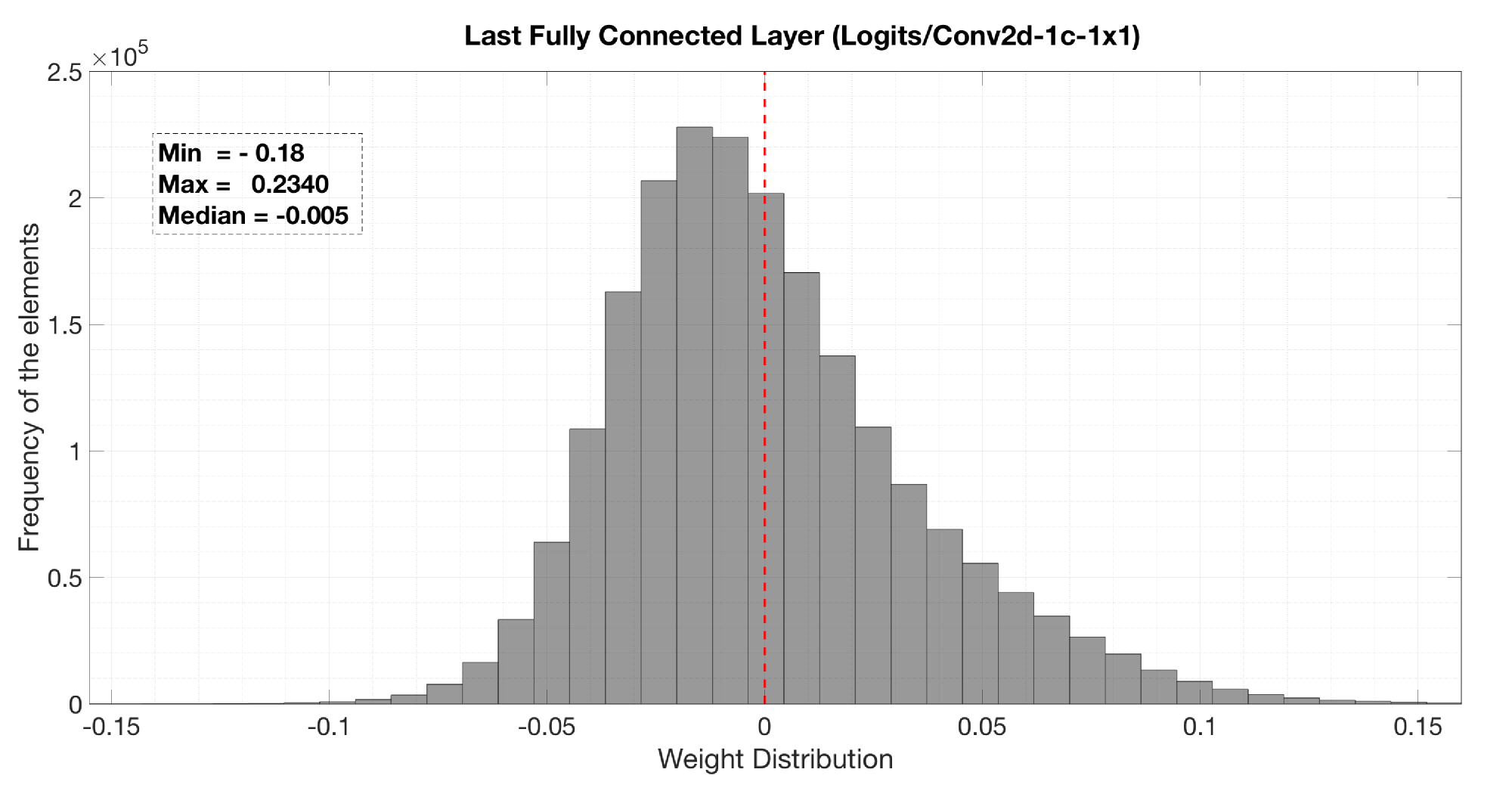
(a) Inception-v3 Softmax

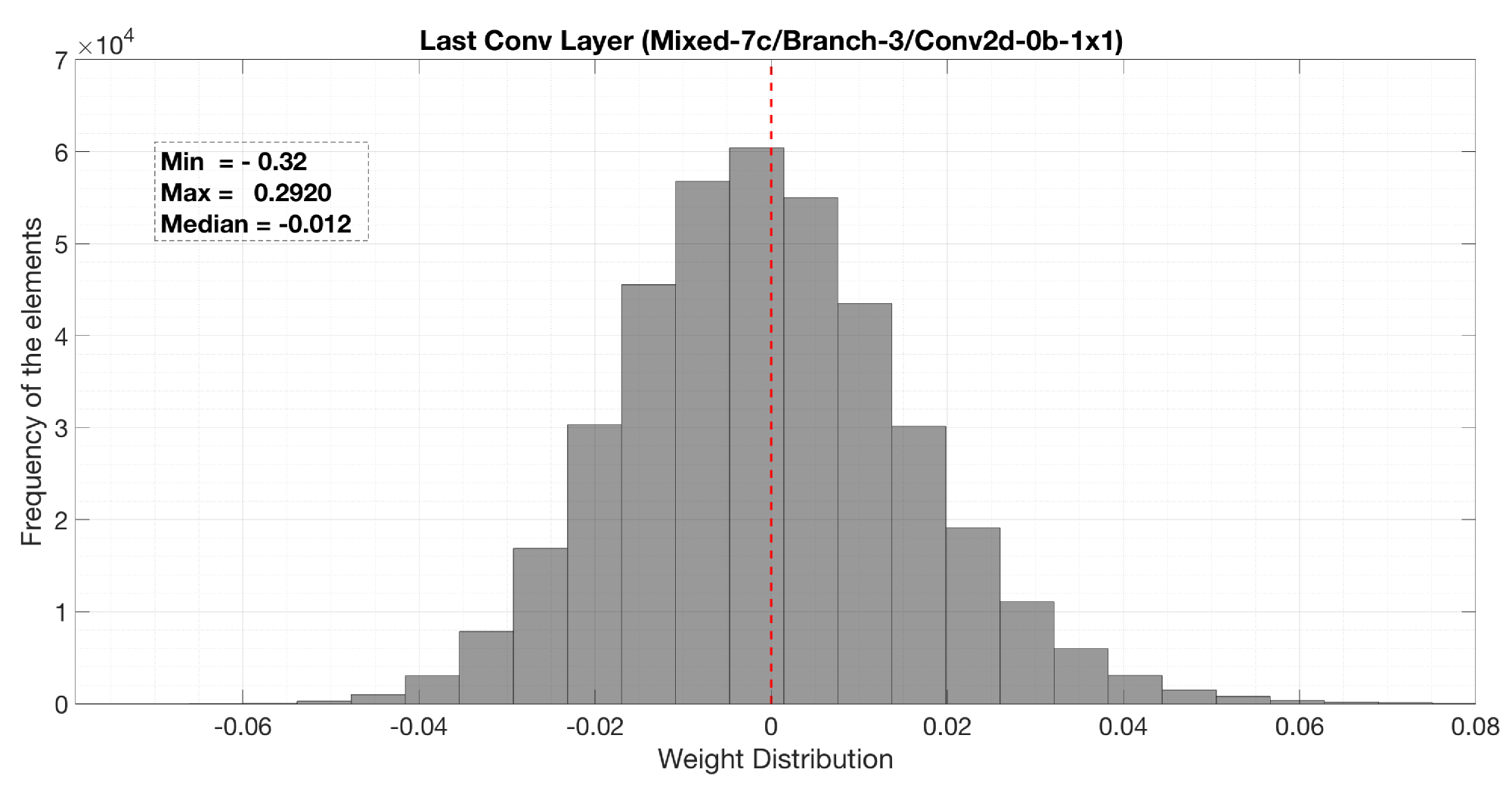
(b) Inception-v3 Last Conv

Figure 1: Distribution of the weights in Inception-v3

The choice of the values of the elements of the vector $T$ defines a sparsification method. These values impact the resulting sparsity and inference accuracy. We define and compare three sparsification methods. The flat method defines a constant threshold $\tau$ for all layers, irrespective of the distribution of their corresponding weights. The triangular method is inspired by the size variation of layers in some state-of-the-art CNNs, where the early layers have smaller number of parameters than latter layers. Finally, the relative method defines a unique threshold for each layer that sparsifies a certain percentage of the weights in the layer. The three methods are depicted graphically in Figure 2a. The high level work-flow of the sparsification framework is depicted in Figure 2b.

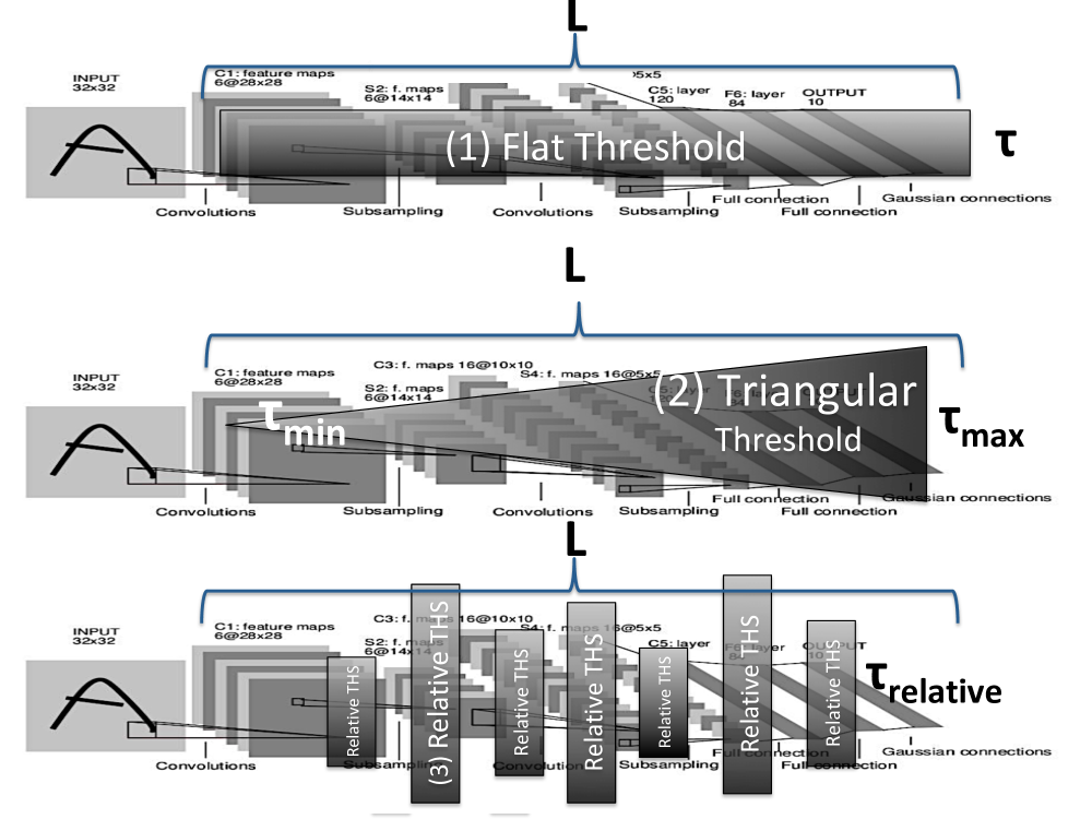
(a) Sparsification Methods

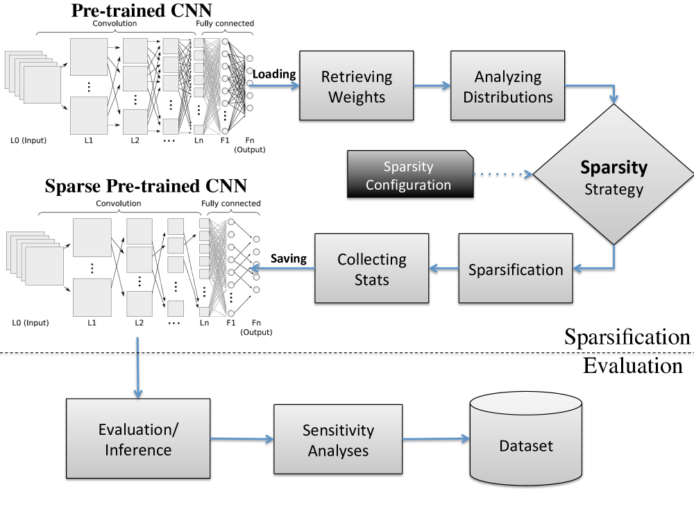
(b) Sparsification Workflow

Figure 2: Proposed Sparsification Framework

3.1 Flat Method

This method defines a constant threshold $\tau$ for all layers, irrespective of the distribution of their corresponding weights. It is graphically depicted in the top of Figure 2a. The weights of the layers are profiled to determine the span $\sigma_{min}=\underset{\forall linL}{min}(max(\omega_{l})-min(\omega_{l}))$. This span corresponds to the layer $k$ having the smallest range of weights within the pretrained model. This span is used as an upper-bound value for our flat threshold $\tau$. Since using $\sigma_{min}$ as a threshold eliminates all the weights in layer $k$ and is likely to adversely affect the accuracy of the sparsified model, we use a fraction $\delta$, $0\leq\delta\leq 1$, of the span:

$$\tau_{l}=\sigma_{min}\times{\delta}$$ (2)

where $\delta$ is a parameter of the method that can be varied to achieve different degrees of model sparsity.

3.2 Triangular Method

The triangular method is inspired by the size variation of layers in state-of-the-art CNNs: early Conv layers have a smaller number of parameters than in later layers, i.e., final Conv and FC layers.

Thus, the triangular sparsification method introduces the highest sparsity in the final layers and gradually diminishes the sparsification towards the early layers. This is done using an isosceles triangular shape for the values of the thresholds, as shown in Figure 2a. This not only caters to the size variation of layers, it also avoids aggressive sparsification in early layers, which can adversely impact subsequent layers because pruning too many neurons in earlier layers can effectively remove many paths in layers further down.

The triangular method is defined by two thresholds $\tau_{min}$ and $\tau_{max}$ for respectively the first convolution layer (i.e, layer 1) and the last fully connected layer (i.e., layer $L$). They represent the thresholds at the tip and the base of the triangle in middle part of Figure 2a. These thresholds are determined by the span of the weights in each of the two layers. Thus,

$$\tau_{min}=\sigma_{conv}*\delta_{conv}$$ (3)

$$\tau_{max}=\sigma_{fc}*\delta_{fc}$$

where $\sigma_{conv}$ is the span of the weights in the first convolution layer, defined in a similar way as for the flat method, and it represents an upper bound on $\tau_{min}$. Thus, $\delta_{conv}$ is a fraction that ranges between $0$ and $1$. Similarly, $\sigma_{fc}$ is the span of the weights in the last fully connected layer and it represents an upper bound on $\tau_{max}$. Thus, $\delta_{fc}$ is a fraction that ranges between $0$ and $1$.

The thresholds of the remaining layers are dictated by the position of these layers in the network. Thus, the $\tau$ value for each layer $l$, $1\leq l\leq L$, is given by:

$$\tau_{l}=\begin{cases}\tau_{min}&\text{if}~{}~{}~{}~{}~{}\ l=1\\ \tau_{max}&\text{if}~{}~{}~{}~{}~{}\ l=L\\ \dfrac{\tau_{max}-\tau_{min}}{L}\times(l-2)&\text{Otherwise}\end{cases}$$ (4)

3.3 Relative Method

Several state-of-the-art CNNs, such as Inception-v3 [31] or AlexNet [15] no longer exhibit a linear expansion in the design of their layers’ parameters. Rather, they exhibit a more complex structure in which bigger layers are replaced by multiple smaller layers that are grouped together. To this end, a flat or triangular sparsification method might not be intuitive and efficient because it can aggressively prune smaller and under-sparsify wider layers.

The relative method attempts to address this issue. It defines a unique threshold for each layer that is solely based on the distribution of the weights of that layer. The value of $\tau_{l}$ is picked such that it is the $\delta_{l}$th percentile of the weights in layer $l$. That is, $\tau_{l}$ is a value such that approximately $\delta_{l}$ of the weights (in absolute value) are less than or equal to $\tau_{l}$. Thus, our sparsification function (Equation 1) results in approximately $\delta_{l}$ zeros for layer $l$.

In particular, it uses the $\delta^{th}$ percentile of distribution’s weight in layer $l$ denoted by $\delta_{l}$. Thus each element of the vector $T(l)=\tau_{l}$ is defined as:

$$\tau_{l}=(max(\omega_{l})-min(\omega_{l}))\times{\delta_{l}}$$ (5)

where $0\leq\delta_{l}\leq 1$ defines the desired percentile of the $\delta_{l}$ of zero weights in each layers.

4 Experimental Evaluation and Comparison

Figure 2b depicts the highlevel flow of our proposed sparsification framework. A pretrained CNN is first loaded, as shown on the upper left side of the figure. The meta-graph and the weights of the model are then retrieved. Next, the histogram of the weights in each layer is generated, and the threshold value(s) of the sparsification method used are determined. Once the method is applied, the sparsified weights are saved as a new sparsified version of the CNN. The sparsified model is then evaluated to capture its new inference accuracy. Note that on an industrial use case such as an app on a Mobile device, the pretrained models are embedded into the app and only communicate with the API using a library. Thus, our method can also be applied on-the-fly and sparsifies the loaded weights as they are appended to the device memory and just before the execution.

We evaluate our sparsification methods using TensorFlow v1.4 with CUDA runtime and driver v8. The evaluation of Top-5 accuracy is done on an NVIDIA’s GeForce GTX 1060 with a host running Ubuntu 14.04, kernel v3.19 using ImageNet ([14]).

Metrics

We evaluate our sparsified models using two key metrics. The first is the model sparsity ratio, as defined in Section 3. We use it as a proxy for the amount of memory and computation (i.e, number of MACs) savings possible when sparsity is exploited. While the savings will not equal the sparsity ratio (because of compression overheads), the extent to which these savings introduce remains proportional to the ratio. does not explicitly reflect the quantitative value saved by a sparsified model, nevertheless, it hints the compression’s potential of a model to be exploited later by canceling the multiplications and addition of 0s. The second metric is the drop in inference accuracy. The acceptable drop in inference accuracy is highly application dependent. In our evaluation, we set the acceptability threshold for normalized inference accuracy to 95%. We explore sparsification methods that result in the largest model sparsity within this threshold.

Figures 3a, 3b, 3c, 3d, and 3e show the inference accuracy as a function of the introduced sparsity by each method. They reflect that significant sparsity can be obtained with a small reduction in inference accuracy. With less than 5% reduction in accuracy, we gain 51% sparsity (2.04$\times$ compression factor), 50% (2$\times$), 62% (2.63$\times$), 70% (3.33$\times$), and 73% (3.7$\times$) for the models. This validates our approach.

Further, the figures reflect that the relative method outperforms the other two methods for the Inception-v3, VGG and ResNet, but the triangular one outperforms the other two for MobileNet-v1 This is likely due to the structure of the models. MobileNet-v1 and Alexnet have a gradual linear increase in the size of the convolution layers, making the triangular method more effective. In contrast, the other models have no such increase, making the relative method more effective. As a case-in-point, ResNet has 152 conv layers with variable sizes, which makes the triangular method less effective, as seen by the drop in accuracy in Figure 3c.

An interesting observation is that for Alexnet, introducing the first 50% sparsity suffers little drop in accuracy. This value is 35%, 30%, 41%, and 42% for the other models and it shows there exists significant redundancy within CNNs. Han et al. [6] observe the same with their Caffe implementation of Alexnet. The work was mainly focused on iteratively pruning and retraining CNNs to compensate the loss of accuracy. The authors’ method with no retraining is not specified and it is unclear if it applies to other CNNs or not. However, the authors report a gain of around 80% sparsity by pruning (i.e., without retraining) Alexnet with L2 regularization. Our evaluation validates their result across other models using the proposed on-the-fly methods.

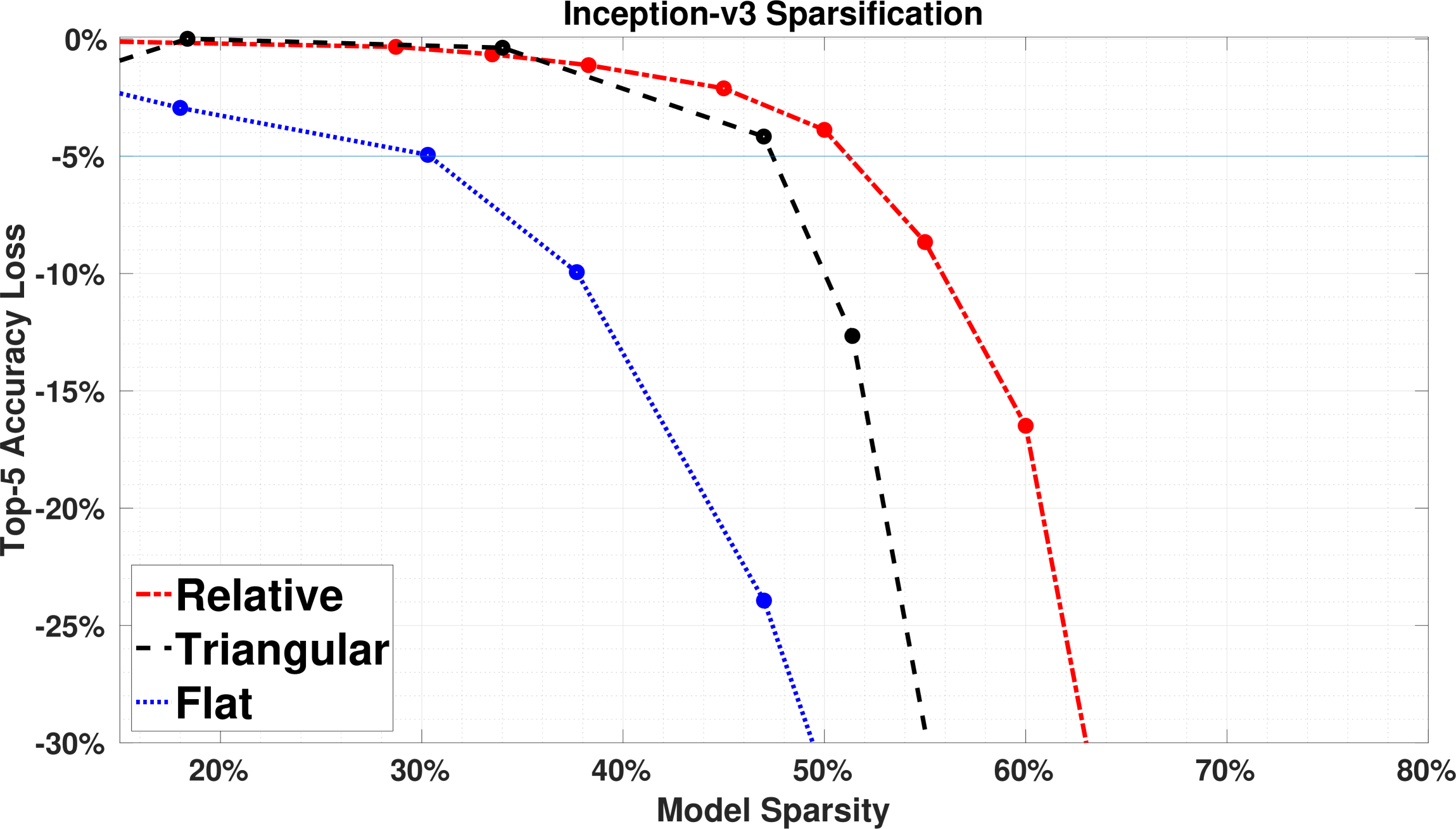
(a) Inception-v3

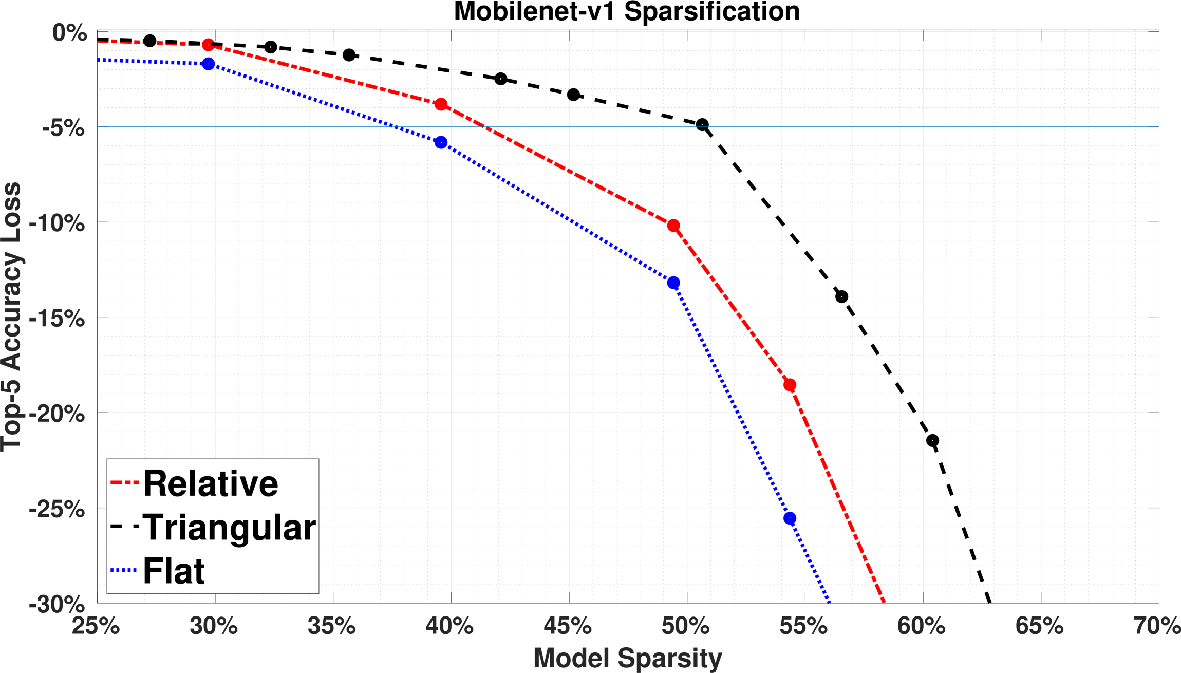
(b) MobileNets-v1

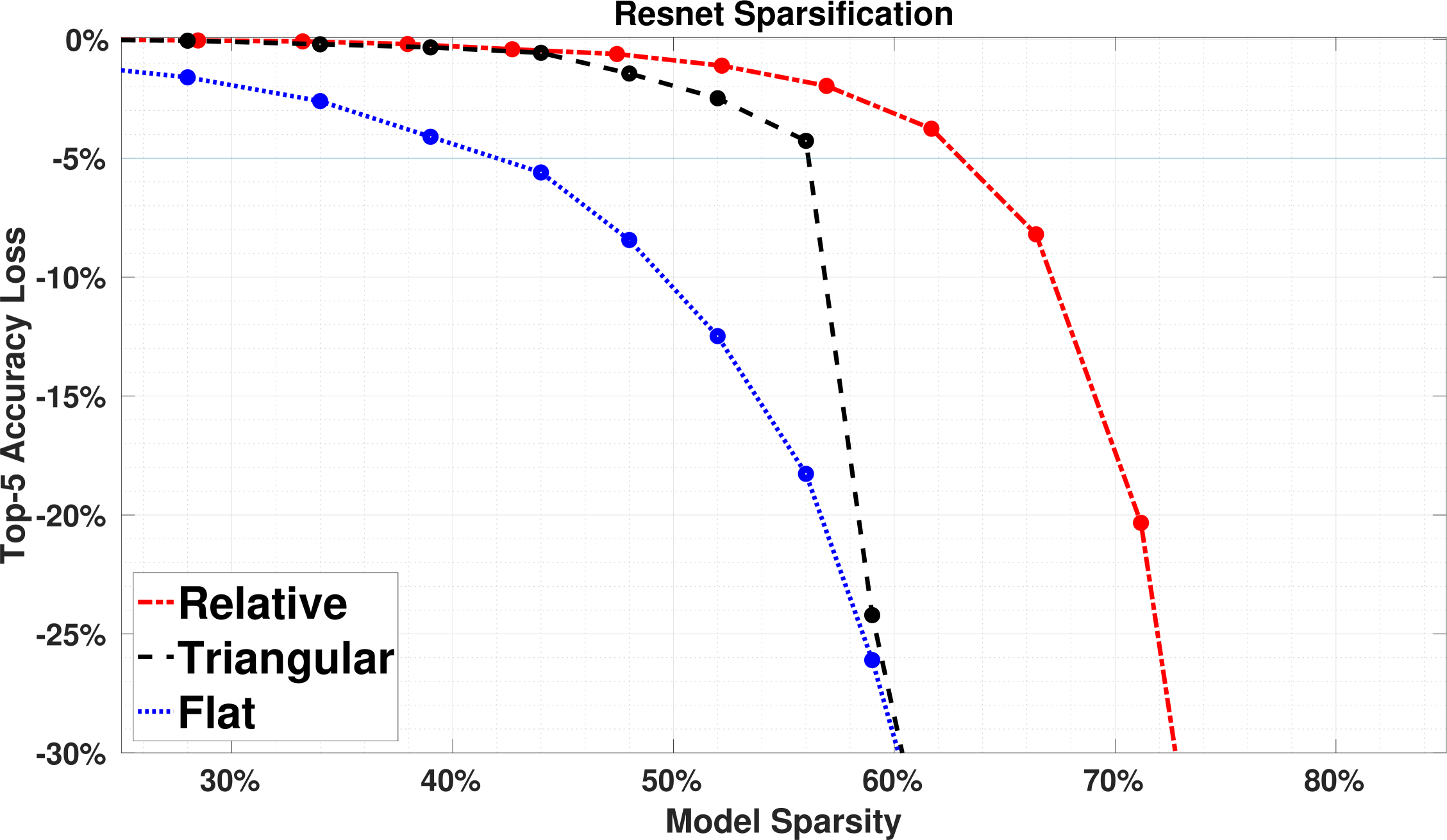
(c) ResNet-v2

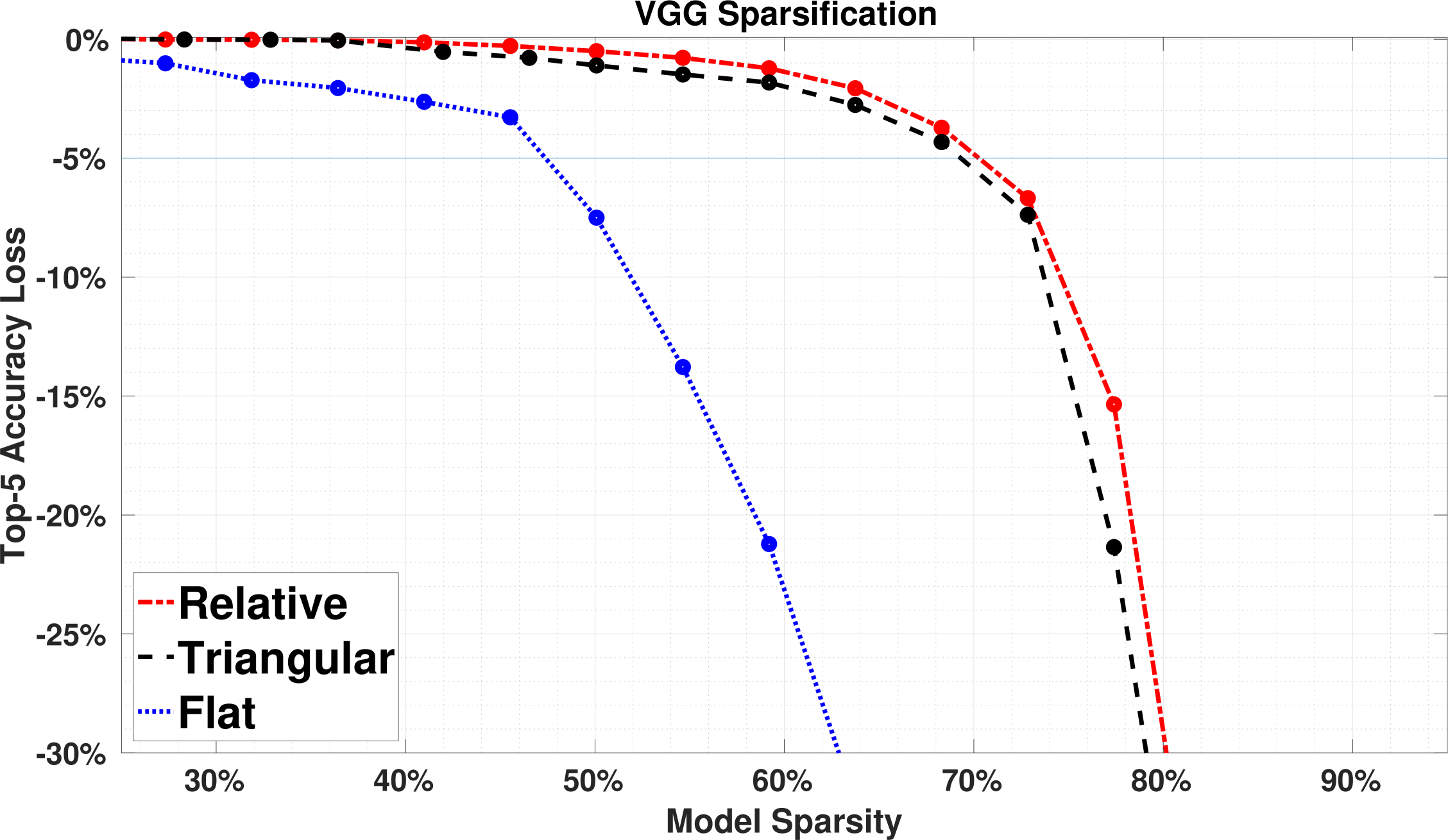
(d) VGG-16

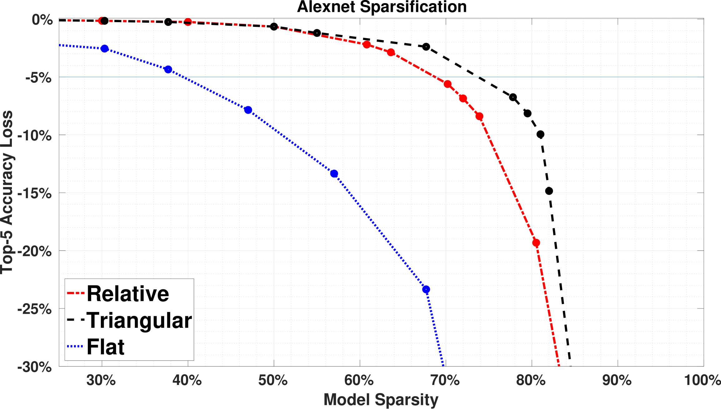
(e) Alexnet

Layers	#Params	%Sparsified
Conv1	23 K	10%
Conv2	307K	35%
Conv3	663K	35%
Conv4	1.3M	35%
Conv5	884K	35%
FC1	26M	85%
FC2	16M	85%
FC3	4M	73%
Total	50M	81.1%

(f) Alexnet Fine-tuning

Figure 3: Sparsity-Accuracy Trade-off for Our Three Proposed Sparsification Methods

Fine-tuning. We explore what can be achieved by some fine-tuning of our methods, still with no retraining, in order to gain more sparsity. We do so to determine the effectiveness of our on-the-fly methods, since the fine-tuning is not likely feasible in out context. We focus on the relative method and start with a baseline sparsity. We then vary the degree of sparsity of each layer in turn around the base sparsity, attempting to maintain a no more than 5% drop in inference accuracy. The results for AlexNet are shown in the table in Figure 3f. The baseline sparsity is selected as 70%. It is possible for some layers, particularly larger ones, to have higher sparsity, while smaller layers are more sensitive to sparsification and must have lower sparsity. Nonetheless, there is a gain of 8% in overall model sparsity. This value is 4%, 3%, 2% , and 5% for Inception-v3, Mobilenet-v1, ResNet, and VGG, respectively. Since this gain comes at the expense of an exploration of different sparsity ratios for the layers and thus more computations, it is not feasible in the contexts we explore. However, the gain is not significant to render our on-the-fly methods inefficient on their own without further tuning.

5 Concluding Remarks

We explored sparsification without retraining of CNNs and proposed three model-independent methods doing so. We experimentally evaluated these methods and showed that they can result in up to 73% sparsity with less than 5% drop in inference accuracy. However, there is no single method that works best for all models. Further, our evaluation showed that it is possible to fine-tune the methods to further gain sparsity with no significant drop in inference accuracy. However, such tuning of the methods is complex and suggests the need for autotuning. There are two key directions for future work. The first is to explore heuristics for selecting a sparsification method based on the CNN model and possibly fine tune the parameters of the methods. Identifying the best sparsity configuration is important and the choice of the right sparsification method, the layers to target, and the sparsity ratio for each targeted layer presents an optimization problem. The second is to realize the benefit of the sparsity in the model’s implementation on the NNlib library, which offloads neural networks operations from TensorFlow to Qualcomm’s Hexagon-DSP. The introduction of zeros in the model weights can only benefit performance/energy if their presence is exploited. In particular, we also wish to address the additional challenge that arises in the quantized model, which stems from the fact that the representation of a zero is neither the value zero nor is unique. Thus, we will explore different quantization approaches to address this shortcoming.

References

- [1] Sajid Anwar, Kyuyeon Hwang, and Wonyong Sung. Fixed point optimization of deep convolutional neural networks for object recognition. In 2015 IEEE Int. Conf. Acoust. Speech Signal Process., pages 1131–1135. IEEE, apr 2015.
- [2] Amir H. Ashouri, William Killian, John Cavazos, Gianluca Palermo, and Cristina Silvano. A survey on compiler autotuning using machine learning. ACM Comput. Surv., 51(5):96:1–96:42, September 2018.
- [3] Yann Le Cun, John S Denker, and Sara a Solla. Optimal Brain Damage. Adv. Neural Inf. Process. Syst., 2(1):598–605, 1990.
- [4] Xin Dong, Shangyu Chen, and Sinno Jialin Pan. Learning to Prune Deep Neural Networks via Layer-wise Optimal Brain Surgeon. NIPS, pages 4860–4874, may 2017.
- [5] Song Han, Xingyu Liu, Huizi Mao, Jing Pu, Ardavan Pedram, Mark A. Horowitz, and William J. Dally. EIE: Efficient Inference Engine on Compressed Deep Neural Network. In Proc. - 2016 43rd Int. Symp. Comput. Archit. ISCA 2016, pages 243–254. IEEE, jun 2016.
- [6] Song Han, Huizi Mao, and William J. Dally. Deep Compression: Compressing Deep Neural Networks with Pruning, Trained Quantization and Huffman Coding. arXiv Prepr. arXiv1510.00149, oct 2015.
- [7] Song Han, Jeff Pool, John Tran, and William J. Dally. Learning both Weights and Connections for Efficient Neural Networks. papers.nips.cc, 2015.
- [8] Tianyi David Han and Tarek S Abdelrahman. Automatic tuning of local memory use on gpgpus. arXiv preprint arXiv:1412.6986, 2014.
- [9] Babak Hassibi and David Stork. Second order derivaties for network prunning: Optimal brain surgeon. In Nips, pages 164–171, 1993.
- [10] Kaiming He, Xiangyu Zhang, Shaoqing Ren, and Jian Sun. Deep Residual Learning for Image Recognition. In 2016 IEEE Conf. Comput. Vis. Pattern Recognit., pages 770–778, 2016.
- [11] Geoffrey Hinton, Oriol Vinyals, and Jeff Dean. Distilling the knowledge in a neural network. arXiv preprint arXiv:1503.02531, 2015.
- [12] Qiangui Huang, Kevin Zhou, Suya You, and Ulrich Neumann. Learning to Prune Filters in Convolutional Neural Networks. jan 2018.
- [13] Forrest N Iandola, Song Han, Matthew W Moskewicz, Khalid Ashraf, William J Dally, and Kurt Keutzer. SqueezeNet: AlexNet-level accuracy with 50x fewer parameters and< 0.5 MB model size. In arXiv, feb 2017.
- [14] Jia Deng, Wei Dong, R Socher, Li-Jia Li, Kai Li, and Li Fei-Fei. ImageNet: A large-scale hierarchical image database. In 2009 IEEE Conf. Comput. Vis. Pattern Recognit., pages 248–255, 2009.
- [15] Alex Krizhevsky, Ilya Sutskever, and Geoffrey E. Hinton. ImageNet Classification with Deep Convolutional Neural Networks. Adv. Neural Inf. Process. Syst., pages 1–9, 2012.
- [16] Yann LeCun, Léon Bottou, Yoshua Bengio, and Patrick Haffner. Gradient-based learning applied to document recognition. Proceedings of the IEEE, 86(11):2278–2324, 1998.
- [17] Weiwei Liu, Xiaobo Shen, and Ivor Tsang. Sparse Embedded k-Means Clustering. Adv. Neural Inf. Process. Syst. 30, (Nips):3321–3329, 2017.
- [18] Huizi Mao, Song Han, Jeff Pool, Wenshuo Li, Xingyu Liu, Yu Wang, and William J. Dally. Exploring the Granularity of Sparsity in Convolutional Neural Networks. In IEEE Comput. Soc. Conf. Comput. Vis. Pattern Recognit. Work., volume 2017-July, pages 1927–1934, may 2017.
- [19] Huizi Mao, Song Han, Jeff Pool, Wenshuo Li, Xingyu Liu, Yu Wang, and William J. Dally. Exploring the Regularity of Sparse Structure in Convolutional Neural Networks. arXiv Prepr. arXiv1705.08922, may 2017.
- [20] Manu Mathew, Kumar Desappan, Pramod Kumar Swami, and Soyeb Nagori. Sparse, Quantized, Full Frame CNN for Low Power Embedded Devices. In IEEE Comput. Soc. Conf. Comput. Vis. Pattern Recognit. Work., volume 2017-July, pages 328–336, 2017.
- [21] Cameron Musco and David P Woodruff. Is Input Sparsity Time Possible for Kernel Low-Rank Approximation? In NIPS, number Nips, 2017.
- [22] Vlad Niculae and Mathieu Blondel. A Regularized Framework for Sparse and Structured Neural Attention. papers.nips.cc, 2017.
- [23] Angshuman Parashar, Minsoo Rhu, Anurag Mukkara, Antonio Puglielli, Rangharajan Venkatesan, Brucek Khailany, Joel Emer, Stephen W. Keckler, William J. Dally, Angshuman Parashar, Minsoo Rhu, Anurag Mukkara, Antonio Puglielli, Rangharajan Venkatesan, Brucek Khailany, Joel Emer, Stephen W. Keckler, and William J. Dally. SCNN: An Accelerator for Compressed-sparse Convolutional Neural Networks. In Proc. 44th Annu. Int. Symp. Comput. Archit. - ISCA ’17, volume 45, pages 27–40, New York, New York, USA, 2017. ACM Press.
- [24] Karen Simonyan and Andrew Zisserman. Very Deep Convolutional Networks for Large-Scale Image Recognition. Int. Conf. Learn. Represent., pages 1–14, sep 2015.
- [25] Suraj Srinivas, Akshayvarun Subramanya, and R. Venkatesh Babu. Training Sparse Neural Networks. In IEEE Comput. Soc. Conf. Comput. Vis. Pattern Recognit. Work., volume 2017-July, pages 455–462, 2017.
- [26] Nitish Srivastava, Geoffrey Hinton, Alex Krizhevsky, Ilya Sutskever, and Ruslan Salakhutdinov. Dropout: A Simple Way to Prevent Neural Networks from Overfitting. J. Mach. Learn. Res., 15:1929–1958, 2014.
- [27] Yi Sun, Xiaogang Wang, and Xiaoou Tang. Sparsifying Neural Network Connections for Face Recognition. In 2016 IEEE Conf. Comput. Vis. Pattern Recognit., pages 4856–4864. IEEE, jun 2016.
- [28] Vivienne Sze, Yu-Hsin Chen, Tien-Ju Yang, and Joel S. Emer. Efficient Processing of Deep Neural Networks: A Tutorial and Survey. Proc. IEEE, 105(12):2295–2329, dec 2017.
- [29] Christian Szegedy, Sergey Ioffe, Vincent Vanhoucke, and Alexander A Alemi. Inception-v4, inception-resnet and the impact of residual connections on learning. In AAAI, volume 4, page 12, 2017.
- [30] Christian Szegedy, Wei Liu, Yangqing Jia, Pierre Sermanet, Scott Reed, Dragomir Anguelov, Dumitru Erhan, Vincent Vanhoucke, and Andrew Rabinovich. Going deeper with convolutions. In Proc. IEEE Comput. Soc. Conf. Comput. Vis. Pattern Recognit., volume 07-12-June, pages 1–9. IEEE, jun 2015.
- [31] Christian Szegedy, Vincent Vanhoucke, Sergey Ioffe, Jonathon Shlens, and Zbigniew Wojna. Rethinking the Inception Architecture for Computer Vision. arXiv, dec 2015.
- [32] Wei Wen, Chunpeng Wu, Yandan Wang, Yiran Chen, and Hai Li. Learning Structured Sparsity in Deep Neural Networks. Nature, 521(12):61–4, 2016.
- [33] Xiyu Yu, Tongliang Liu, Xinchao Wang, and Dacheng Tao. On Compressing Deep Models by Low Rank and Sparse Decomposition. In 2017 IEEE Conf. Comput. Vis. Pattern Recognit., pages 67–76. IEEE, jul 2017.
- [34] Yongqiang Zhang. Low-Rank-Sparse Subspace Representation for Robust Regression. Cvpr, pages 7445–7454, 2017.