Spin-valley half-metal in systems with Fermi surface nesting

Abstract

Half-metals have fully spin polarized charge carriers at the Fermi surface. Such polarization usually occurs due to strong electron–electron correlations. Recently [Phys. Rev. Lett. 119, 107601 (2017)], we have demonstrated theoretically that adding (or removing) electrons to systems with Fermi surface nesting also stabilizes the half-metallic states even in the weak-coupling regime. In the absence of doping, the ground state of the system is a spin or charge density wave, formed by four nested bands. Each of these bands is characterized by charge (electron/hole) and spin (up/down) labels. Only two of these bands accumulate charge carriers introduced by doping, forming a half-metallic two-valley Fermi surface. Analysis demonstrates that two types of such half-metallicity can be stabilized. The first type corresponds to the full spin polarization of the electrons and holes at the Fermi surface. The second type, with antiparallel spins in electron-like and hole-like valleys, is referred to as a “spin-valley half-metal” and corresponds to the complete polarization with respect to the spin-valley operator. We analyze spin and spin-valley currents and possible superconductivity in these systems. We show that spin or spin-valley currents can flow in both half-metallic phases.

I Introduction

Electron states at the Fermi surface of usual metals are degenerate with respect to the spin projection. Consequently, the spin polarization of such electron systems is zero. However, strong electron-electron interactions can lift this degeneracy and thus, the electron liquid at the Fermi surface acquires spin polarization. In the most extreme case, electrons with only one spin projection (spin-up or spin-down) reach the Fermi surface, while the states with opposite spin projection are pushed away from the Fermi energy. These systems are referred to as half-metals de Groot et al. (1983); Katsnelson et al. (2008); Hu (2012). The most immediate consequence of the half-metallicity is the perfect spin polarization of the electric current. This makes half-metals promising materials for applications in spintronics Žutić et al. (2004); Hu (2012). Many rather different materials are now classified as half-metals; for example: NiMnSb, Hanssen et al. (1990) La_0.7Sr_0.3MnO₃, Park et al. (1998) CrO₂, Ji et al. (2001) Co₂MnSi, Jourdan et al. (2014) among others. Along with the listed above ferromagnets, the half-metallicity can exist in the systems with different magnetic ordering. In Ref. M. P. Ghimire, using the first-principles density functional approach, it was shown that in double-perovskite structure [Pr_2-xSr_xMgIrO₆]₂ synthesized recently, half-metal antiferromagnetism or ferrimagnetism can be observed depending on the Sr doping level.

It is commonly accepted Katsnelson et al. (2008) that the half-metallicity of the compounds listed above is related to an appreciable electron-electron interaction, associated with the transition-metal atoms. However, in recent years, transition-metal-free half-metallicity has been a subject of intense research activity. As a specific example, one can mention density-functional studies Du et al. (2012); Hashmi and Hong (2014), which predict the existence of half-metallicity in graphitic carbon nitride $g$-C₄N₃. Another well-known suggestion is to look for half-metallicity at the zigzag edges of graphene nanoribbons Son et al. (2006). Some other proposals have also been discussed Kan et al. (2012); Huang et al. (2010). Transition-metal-free half-metals could be of interest for bio-compatible applications and, in general, are consistent with current interest in carbon-based and organic-based mesoscopic systems Soriano and Fernández-Rossier (2010); Klauk (2010); Avouris et al. (2007); Rozhkov et al. (2011); Sa-Ke et al. (2014); Rozhkov et al. (2016). The spin-orbit coupling produces a significant effect on the spin polarization and, consequently, on the condition under which the half-metallicity is observed. In the materials without transition metals, this coupling is small. In our consideration, we neglect spin-orbit interaction since the main idea of our proposal is to demonstrate that the half-metallic state can exist in the systems consisting only of light atoms, when all effects related to heavy atoms are disregarded.

A strong electron-electron interaction is not characteristic of materials composed entirely of $s$- and $p$-elements. Therefore, it is reasonable to focus the search for transition-metal-free half-metals on systems, in which the electrons at the Fermi surface can be completely polarized under the condition of weak electron-electron coupling.

In our recent work, Ref. Rozhkov et al., 2017, we have proposed a mechanism for half-metallicity in the weak-coupling regime. We demonstrated that doping a spin-density wave (SDW) or charge-density wave (CDW) insulator may stabilize a certain type of half-metallic state provided that the undoped system has two nested spin-degenerate Fermi surface sheets, which we will also refer to as valleys. The nesting between the electron and hole Fermi surface sheets makes the system unstable with respect to density wave formation Rozhkov et al. (2017). The SDW or CDW instability opens a gap, giving rise to an insulating ground state. When doping is introduced, the system becomes metallic, with two new Fermi surface sheets Rozhkov et al. (2017). Both sheets are half-metallic. If the spin polarizations of the sheets are parallel to each other, a half-metallic state, denoted below as a CDW half-metal, emerges. For antiparallel polarizations, a different half-metallic state, the SDW or spin-valley half-metal, appears Rozhkov et al. (2017).

In this paper, we present a more detailed analysis of the previously proposed approach Rozhkov et al. (2017) to half-metallicity. The most immediate consequences of the half-metallicity are also discussed. Specifically, we calculate the phase diagram of the model as a function of doping. Then, the relation of the electric current to the spin and spin-valley currents is discussed. Namely, below we show that, depending on the specific parameters, the current carries, in addition to the electric charge, either spin or spin-valley quantum numbers. Finally, the structure of a possible superconducting order parameter is discussed. Since there is no spin degeneracy in a half-metal, but two valleys are available, the superconductivity in such a system is rather different from that of common $s$-wave superconductors.

This paper is organized as follows. In Sec. II we formulate the model, derive its mean field solution, and construct the model’s phase diagram. Both commensurate and incommensurate density wave order parameters are investigated. In Sec. III the conductivity of the system is analyzed. Superconductivity is considered in Sec. IV. Finally, the main results are discussed in Sec. V.

II Model

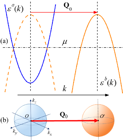
Figure 1: Electron bands of the model when the electron-electron coupling is neglected and doping is zero. (a): Electron band $\varepsilon^{a}({\bf k})$ and hole band $\varepsilon^{b}({\bf k})$ are shown by solid curves. The dashed parabola is the hole band translated by the nesting vector ${\bf Q}_{0}$. The vertical axis is energy and the horizontal axis is momentum, while the Fermi level $\mu$ is shown by the horizontal dash-dot line. (b): Spherical Fermi surfaces of the electron and hole bands. The spheres coincide if we translate one of them by the nesting vector.

We consider here an isotropic two-band electron model. Both bands or valleys have a quadratic dispersion law. Bands $a$ and $b$ are the electron and hole bands, respectively. The bands are schematically shown as blue and orange parabolas in Fig. 1(a). Thus, the single-particle dispersions of the bands can be written as ($\hbar=1$)

$$\varepsilon^{a}(\mathbf{k})=\frac{\mathbf{k}^{2}}{2m_{a}}+\varepsilon^{a}_{\textrm{min}}-\mu,\quad\varepsilon^{a}_{\textrm{min}}<\varepsilon^{a}<\varepsilon^{a}_{\textrm{max}},$$ (1)

$$\varepsilon^{b}(\mathbf{k}\!+\!\mathbf{Q}_{0})=-\frac{\mathbf{k}^{2}}{2m_{b}}+\varepsilon^{b}_{\textrm{max}}-\mu,\quad\varepsilon^{b}_{\textrm{min}}<\varepsilon^{b}<\varepsilon^{b}_{\textrm{max}}.$$ (2)

Here, band $a$ is centered at ${\bf k}=0$, and band $b$ is shifted by some momentum ${\bf Q}_{0}$. Below, for simplicity, we assume perfect electron-hole symmetry: $m_{a}=m_{b}=m$ and $\varepsilon^{b}_{\textrm{max}}=-\varepsilon^{a}_{\textrm{min}}=\varepsilon_{\rm F}$. Zero doping corresponds to $\mu=0$. In the absence of doping, the Fermi surface sheets for the $a$ and $b$ bands are spheres [see Fig. 1(b)] with the same Fermi momentum $k_{\rm F}=\sqrt{2m\varepsilon_{\rm F}}$ and the same density of states (per spin projection) $N_{\rm F}={mk_{\rm F}}/(2\pi^{2})$ at the Fermi energy. A model of this kind was introduced long ago by Rice in connection to the incommensurate SDW in chromium Rice (1970). Hereafter, $\varepsilon_{\rm F}$, $k_{\rm F}$, and $N_{\rm F}$ denote the corresponding values at zero doping.

The quasiparticle dispersion given by Eqs. (1) and (2) exhibits perfect nesting; that is, after translating the electron Fermi surface by the vector $\mathbf{Q}_{0}$, the electron sheet completely coincides with the hole sheet, see Fig. 1. The vector $\mathbf{Q}_{0}$ is usually referred to as the nesting vector.

In general, electrons interact with each other, so the total Hamiltonian of the system is

$$\hat{H}=\hat{H}_{e}+\hat{H}_{\textrm{int}}\,.$$ (3)

Here $\hat{H}_{e}$ is the one-electron term, which corresponds to the dispersion laws (1) and (2). The term $\hat{H}_{\textrm{int}}$ describes the interaction between quasiparticles.

We are interested in the weak-coupling regime, as it was mentioned above. We assume that the interband and intraband interactions are of the same order. Thus, to treat the SDW or CDW instability, it is sufficient to keep in $H_{\rm int}$ only the interaction between the electrons in band $a$ and holes in band $b$, respectively Rice (1970); Rozhkov et al. (2017). It is this term in the interaction Hamiltonian, which generates the gap and cannot be treated as a perturbation. A weak intraband coupling can be considered perturbatively, but this can be safely neglected because it only provides small corrections to our results. This common feature of BCS-like approaches can be proved by a direct calculation.

Below we assume that the interaction is a short-range one. In this case, $\hat{H}_{\textrm{int}}$ can be written as

$$\hat{H}_{\textrm{int}}=\hat{H}_{\textrm{dir}}+\hat{H}_{\textrm{ex}},$$ (4)

where

$$\hat{H}_{\textrm{dir}}\!=\!g\int\!{d^{3}{\bf r}\,\sum_{\sigma\sigma^{\prime}}\psi^{\dagger}_{a\sigma}(\mathbf{r})\,\psi^{\vphantom{\dagger}}_{a\sigma}(\mathbf{r})\,\psi^{\dagger}_{b\sigma^{\prime}}\!(\mathbf{r})\,\psi^{\vphantom{\dagger}}_{b\sigma^{\prime}}\!(\mathbf{r})}\,,$$ (5)

and

$$\hat{H}_{\textrm{ex}}\!=\!g_{\perp}\int\!d^{3}\mathbf{r}\,\sum_{\sigma\sigma^{\prime}}\psi^{\dagger}_{a\sigma}\!(\mathbf{r})\psi_{b\sigma}^{\vphantom{\dagger}}(\mathbf{r})\psi^{\dagger}_{b\sigma^{\prime}}\!(\mathbf{r})\psi_{a\sigma^{\prime}}^{\vphantom{\dagger}}(\mathbf{r})\,.$$ (6)

Here, $\psi_{\alpha\sigma}\!(\mathbf{r})$ denotes the usual fermionic field operator for band $\alpha$ ($=a,b$) and spin projection $\sigma$ onto the $z$ axis; and ${\bf r}$ refers to spatial coordinates. The term $\hat{H}_{\textrm{dir}}$ represents the direct part of the density-density interaction, while $\hat{H}_{\textrm{ex}}$ corresponds to the exchange part of this interaction. The constants $g$ and $g_{\perp}$ describe the electron-hole interaction. We assume that the interaction is repulsive ($g,\,g_{\perp}>0$) and weak ($gN_{\rm F},\,g_{\perp}N_{\rm F}\ll 1$).

II.1 SDW instability and spin-valley half-metal

Hamiltonian (3) can be used to describe the spontaneous formation of low-temperature density-wave order when the Fermi surface sheets of holes and electrons perfectly match each other (perfect nesting). We start with the SDW. Looking ahead, we can state that the SDW order has a lower free energy than the CDW one if we take into account only electron-electron coupling Eqs. (5) and (6), and disregard, say, electron-lattice interactions. Up to rotations of the spin-polarization axis, the SDW ground state is believed to be unique. In the weak-coupling regime, it is well described by a mean-field BCS-like theory.

To construct a mean-field theory of the SDW order, we group the electron operators into two sectors, labeled by the spin index $\sigma=\pm 1/2$ (or $\sigma=\uparrow,\,\sigma=\downarrow$): sector $\sigma$ consists of $\psi_{a\sigma}$ and $\psi_{b{\bar{\sigma}}}$ (here ${\bar{\sigma}}$ means $-\sigma$). In the zero-temperature mean-field approach, the sectors are decoupled, and the (sector-dependent) SDW order parameter is

$$\Delta_{\sigma}=\frac{g}{V}\sum_{\mathbf{k}}\left\langle\psi^{\dagger}_{\mathbf{k}a\sigma}\,\psi^{\phantom{{\dagger}}}_{\mathbf{k}b\bar{\sigma}}\right\rangle\,,$$ (7)

where $V$ is the system volume, and $\langle\ldots\rangle$ denotes the diagonal matrix element for the ground state. The symbol $\psi^{\vphantom{\dagger}}_{\mathbf{k}\alpha\sigma}$ is the Fourier transform of the operator $\psi_{\alpha\sigma}^{\vphantom{\dagger}}(\mathbf{r})$, in which the momentum ${\bf k}$ is measured from the center of the band $\alpha$. The latter convention simplifies the notation; however, one must remember that the centers of the band $a$ and band $b$ are separated by the nesting vector ${\bf Q}_{0}$. Consequently, the order parameter $\Delta_{\sigma}$ oscillates in space with a period related to the wave vector ${\bf Q}_{0}$.

Following a mean-field approach, it is straightforward to check that only the direct interaction (5) contributes to the SDW ordering. The exchange term, Eq. (6), cannot be expressed as a product of two bilinear combinations of the form $\psi^{\dagger}_{a\sigma}\,\psi^{\phantom{{\dagger}}}_{b\bar{\sigma}}$, which enter the definition of order parameter (7). Therefore, $\hat{H}_{\rm ex}$ can be neglected in the lowest approximation, similar to the intravalley terms. Thus, in the mean-field approximation, the model Hamiltonian can be rewritten as

$$\hat{H}_{\textrm{SDW}}\!=\!\sum_{\mathbf{k}\alpha\sigma}\!\left[\varepsilon^{\alpha}(\mathbf{k})\psi_{\mathbf{k}\alpha\sigma}^{{\dagger}}\psi_{\mathbf{k}\alpha\sigma}^{\vphantom{\dagger}}\!-\!\Delta_{\sigma}\psi^{\dagger}_{\mathbf{k}\bar{\alpha}\bar{\sigma}}\psi_{\mathbf{k}\alpha\sigma}^{\vphantom{\dagger}}\!+\!\frac{\Delta_{\sigma}^{2}}{g}\right],$$ (8)

where $\alpha=a,b$ and $\bar{\alpha}$ means ‘not $\alpha$’. The spectrum of Hamiltonian (8) is

$$E^{(1,2)}_{\mathbf{k}\sigma}=\mp\sqrt{\varepsilon^{2}_{\mathbf{k}}+\Delta_{\sigma}^{2}},$$ (9)

where $\varepsilon_{\mathbf{k}}=k^{2}/2m-\varepsilon_{F}$.

The equilibrium parameters of the system can be derived by minimizing the grand thermodynamic potential, defined for arbitrary temperature $T$ by the usual formula

$$\Omega=-T\ln{\!\left\{\textrm{Tr}\,\exp[{-(\hat{H}-\mu\hat{N})/T}]\right\}}.$$ (10)

In this expression, $\hat{N}$ is the operator of the total particle number and the Boltzmann constant $k_{\textrm{B}}=1$. In the mean-field approach, the grand potential of our system is a sum $\Omega=\sum_{\sigma}\Omega_{\sigma}$, where the partial grand potentials $\Omega_{\sigma}$ are equal to Rozhkov et al. (2017)

$$\!\!\Omega_{\sigma}\!=\!\frac{\Delta_{\sigma}^{2}V}{g}\!-\!\sum_{\bf k}\!\left[\mu-E_{{\bf k}\sigma}^{(1)}\!+\!\left(\mu\!-\!E_{{\bf k}\sigma}^{(2)}\right)\theta\!\left(\mu\!-\!E_{{\bf k}\sigma}^{(2)}\right)\!\right].$$ (11)

The symbol $\theta(z)$ denotes the Heaviside step function. To describe the system at finite doping $x$ it is convenient to introduce the partial dopings

$$x_{\sigma}=-\frac{\partial\Omega_{\sigma}}{\partial\mu},$$ (12)

which are the amounts of additional charge accumulated in sector $\sigma$. Obviously, they satisfy

$$x_{\uparrow}+x_{\downarrow}=x\,.$$ (13)

The order parameter $\Delta_{\sigma}$ minimizes the grand potential, $\Omega_{\sigma}(\Delta_{\sigma})$:

$$\frac{\partial\Omega_{\sigma}}{\partial\Delta_{\sigma}}=0.$$ (14)

Thus, to describe the system at finite doping, one has to solve the system of Eqs. (12)–(14) to obtain $\mu$ and $\Delta_{\sigma}$ as functions of $x$. Expressions (11)–(14) are valid provided that the state of the system remains homogeneous, and the SDW order remains commensurate even at finite doping (see Section II.3 and Ref. Rakhmanov et al., 2013). Note here that different electron pockets are usually located near the high-symmetry points of the Brillouin zone. Thus, the vector $\mathbf{Q}_{0}$ is related to the underlying lattice structure and the order may be called commensurate. At nonzero doping, we may try to optimize the energy further by treating the translation vector, $\mathbf{Q}_{1}=\mathbf{Q}_{0}+\mathbf{Q}$, as a variational parameter, which is not directly related to the lattice constant. Further on, such order is referred to as an incommensurate one.

Direct calculations show that, at zero doping, the sectors in the ground state are degenerate: $\Delta_{\uparrow}=\Delta_{\downarrow}=\Delta_{0}$. The nesting is perfect and the order parameter is equal to the BCS-like value

$$\Delta_{0}\approx\varepsilon_{\rm F}\exp\left(-1/gN_{\rm F}\right).$$ (15)

The obvious BCS structure of this expression is a consequence of the fact that in each sector, the mean-field procedure is mathematically equivalent to the BCS calculations.

Once $\Delta_{0}$ is known, the spectrum of the model at $x=0$ can be evaluated, see Fig. 2(a). Note also that at zero doping, the definition of the order parameter Eq. (7) implies that the total SDW polarization in real space is directed along the $x$ axis Rozhkov et al. (2017)

$$\langle S^{x}(\mathbf{r})\rangle = \frac{\Delta_{\uparrow}+\Delta_{\downarrow}}{2g}\exp(i{\bf Q}_{0}{\bf r})+{\rm c.c.}$$

$$= \frac{2\Delta_{0}}{g}\cos({\bf Q}_{0}{\bf r}),$$

$$\langle S^{y}(\mathbf{r})\rangle = \frac{\Delta_{\uparrow}-\Delta_{\downarrow}}{2ig}\exp(i{\bf Q}_{0}{\bf r})+{\rm c.c.}\equiv 0\,.$$ (17)

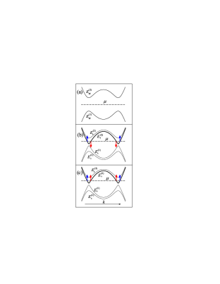
Figure 2: Electron band structure for the insulating and half-metallic states. The vertical axis is the energy, while the horizontal axis is the momentum. The Fermi level $\mu$ is shown by the horizontal dash-dot lines. (a): If doping is zero ($x=0$), the ground state is an insulating SDW or CDW depending on the model parameters, with degenerate sectors ($\Delta_{\uparrow}\equiv\Delta_{\downarrow}$). The energies of electron and hole bands $E_{\sigma}^{(1,2)}$ are given by Eq. (9). (b) and (c): If $x>0$, the sectors are no longer degenerate ($\Delta_{\uparrow}<\mu<\Delta_{\downarrow}\equiv\Delta_{0}$), with the charge accumulating in sector $\uparrow$, in which a Fermi surface appears. The spin polarizations (arrows) of the Fermi surface sheets in (b) correspond to the spin-valley half-metal, and in (c) – to the CDW half-metal.

The doping shifts the chemical potential from zero and suppresses the perfect nesting. The number of low-energy states competing to become the true ground state increases. Both incommensurate and inhomogeneous phases Rice (1970); Gorbatsevich et al. (1992); Eremin and Chubukov (2010); Rakhmanov et al. (2012); Sboychakov et al. (2013a, b, c); Akzyanov et al. (2014); Sboychakov et al. (2017) were considered as ground states of Hamiltonian (3) and its modifications. In our previous paper Ref. Rozhkov et al., 2017, we show that the half-metallic state is yet another viable contender in the case of imperfect nesting. Here, we consider this problem in more detail.

According to Eqs. (12) and (14), the two sectors $\sigma$ are decoupled within the mean-field approach. Then, applying a well-known procedure Gorbatsevich et al. (1992); Rakhmanov et al. (2013); Sboychakov et al. (2017), one can calculate the order parameters $\Delta_{\sigma}$ and the chemical potential $\mu$ as functions of $x_{\sigma}$. This gives the following expression

$$\Delta_{\sigma}=\Delta_{0}\sqrt{1-\frac{x_{\sigma}}{N_{\rm F}\Delta_{0}}}\,,\qquad\mu=\Delta_{0}-\frac{x_{\sigma}}{2N_{\rm F}}\,.$$ (18)

We see that the doping of sector $\sigma$ destroys the order parameter in this sector. In the homogeneous commensurate state, $\Delta_{\sigma}$ is zero when $x_{\sigma}\geq x_{0}$, where

$$x_{0}=N_{\rm F}\Delta_{0}$$ (19)

is a characteristic doping level.

It is usually assumed without extra examination (see, e.g., Refs. Rice, 1970; Rakhmanov et al., 2013; Sboychakov et al., 2017) that the charge carriers are spread evenly between both sectors, that is,

$$x_{\uparrow}=x_{\downarrow}=\frac{x}{2},\quad\text{and}\quad\Delta_{\uparrow}=\Delta_{\downarrow}.$$ (20)

Nevertheless, it is easy to show that the spontaneous lifting of the degeneracy (20) optimizes the energy. To prove this, the system free energy $F$ must be obtained. (Switching from $\Omega$ to $F$ is necessary to work at fixed doping.) The free energy equals to the sum $F=\sum_{\sigma}F_{\sigma}$, where the partial free energy,

$$F_{\sigma}(x_{\sigma})=\Omega_{\sigma}(\mu(x_{\sigma}))+\mu(x_{\sigma})x_{\sigma}$$ (21)

can be calculated as

$$F_{\sigma}(x_{\sigma})=F_{\sigma}(0)+\int\limits_{0}^{\,x_{\sigma}}\!\!dx^{\prime}\mu(x^{\prime})\,,$$ (22)

where

$$F_{\sigma}(0)=-\frac{1}{2}N_{\rm F}\Delta^{2}_{0}$$ (23)

is a well-known BCS-like expression for the free energy at perfect nesting. Then, using $\mu$ from Eq. (18), we derive

$$\frac{F_{\sigma}}{V} = -\frac{N_{\rm F}\Delta^{2}_{0}}{2}+\Delta_{0}x_{\sigma}-\frac{x_{\sigma}^{2}}{4N_{\rm F}}\,,\;\;x_{\sigma}<x_{0}\,,$$ (24)

$$\frac{F}{V} = \sum_{\sigma}\frac{F_{\sigma}}{V}=-N_{\rm F}\Delta_{0}^{2}+\Delta_{0}x-\frac{x_{\uparrow}^{2}+x_{\downarrow}^{2}}{4N_{\rm F}}\,.$$ (25)

Thus, only the third term in Eq. (25) depends on the distribution of the charge between the two sectors. Expression (25) has to be minimized under the constraint (13). It is easy to check that $F$ has the smallest value when $x_{\sigma}=x$ and $x_{\bar{\sigma}}=0$. In other words, for fixed $x$, within the studied class of spatially homogeneous mean-field states, the most stable one corresponds to the case when all the doped charge is accumulated in one sector. The other sector is completely free of extra charge carriers. Thus, the degeneracy between sectors $\sigma=\uparrow$ and $\sigma=\downarrow$ is lifted, and equations (20) are no longer valid. To be specific, let us assume that $\sigma=\uparrow$ represents the sector accumulating extra charge. Therefore, in the ground state, we have

$$\frac{F}{V} = -N_{\rm F}\Delta_{0}^{2}+\Delta_{0}x-\frac{x^{2}}{4N_{\rm F}}\,,$$ (26)

$$\mu = \Delta_{0}-\frac{x}{2N_{\rm F}}\,,$$ (27)

$$\Delta_{\uparrow}(x) = \Delta_{0}\sqrt{1-\frac{x}{N_{\rm F}\Delta_{0}}},\quad\Delta_{\downarrow}(x)=\Delta_{0}\,.$$ (28)

These relations are valid for low doping $x<x_{0}$.

An important feature of Eq. (26) is that the second derivative $\partial^{2}F/\partial x^{2}$ is negative. This means that the doped system may be unstable with respect to electronic phase separation Gorbatsevich et al. (1992); Moreo et al. (1999); Dagotto (2003); Dagotto et al. (2003); Sboychakov et al. (2013b, c); Rakhmanov et al. (2013); Igoshev et al. (2010). However, the long-range Coulomb interaction can suppress phase separation Lorenzana et al. (2001); Bianconi et al. (2015). Thus, it is reasonable to study here the properties of the homogeneous state.

It follows from Eqs. (27) and (28) that

$$\Delta_{\uparrow}(x)<\mu(x)<\Delta_{\downarrow}(x)=\Delta_{0},\,\,\text{when}\,\,0<x<x_{0}.$$ (29)

This means that in the sector $\downarrow$, the order parameter remains equal to $\Delta_{0}$. Since the chemical potential is lower than $\Delta_{\downarrow}$, no charge enters sector $\downarrow$, see Fig. 2(b). In the sector $\uparrow$, two Fermi surface sheets emerge. According to Eqs. (9), (19), (27), and (28), they are determined by

$$\!\!\!\!\!\!\!\varepsilon^{2}_{\bf k}=[\mu(x)]^{2}\!-\![\Delta_{\uparrow}(x)]^{2},\,\,\text{or}\,\,k=k_{\rm F}\sqrt{1\pm\frac{\Delta_{0}}{2\varepsilon_{\rm F}}\frac{x}{x_{0}}}.$$ (30)

The doped state acquires non-trivial macroscopic quantum numbers, since charge carriers introduced by the doping are distributed unevenly between the sectors. To characterize the macroscopic state, it is useful to specify the spin operator ${\hat{S}}$ and spin-valley operator ${\hat{S}}_{\rm v}$:

$${\hat{S}}=\sum_{\alpha\sigma}\sigma{\hat{N}}_{\alpha\sigma},\quad{\hat{S}}_{\rm v}=\sum_{\alpha\sigma}\sigma\nu_{\alpha}{\hat{N}}_{\alpha\sigma},$$ (31)

where

$${\hat{N}}_{\alpha\sigma}=\sum_{\bf k}\psi^{\dagger}_{{\bf k}\alpha\sigma}\,\psi^{\vphantom{\dagger}}_{{\bf k}\alpha\sigma}.$$ (32)

Here, the operator ${\hat{N}}_{\alpha\sigma}$ describes the number of electrons with spin $\sigma$ in valley $\alpha$. The index $\nu_{\alpha}$ is defined according to the rule $\nu_{a}=1$, $\nu_{b}=-1$.

Hamiltonian (3), as well as the mean-field Hamiltonian (8), commutes with both ${\hat{S}}$ and ${\hat{S}}_{\rm v}$. The field operators satisfy obvious commutation rules

$$[{\hat{S}},\psi_{\alpha\sigma}]=\sigma\psi_{\alpha\sigma},\qquad[{\hat{S}}_{\rm v},\psi_{\alpha\sigma}]=\sigma\nu_{\alpha}\psi_{\alpha\sigma}.$$ (33)

Namely, in addition to the usual spin-projection quantum number $\sigma$, the field $\psi_{\alpha\sigma}$ can be characterized by the spin-valley projection $\sigma\nu_{\alpha}$.

Using Eqs. (33), it is easy to check that in the sector $\sigma$, both $\psi_{a\sigma}$ and $\psi_{b{\bar{\sigma}}}$ carry the same spin-valley quantum number equal to $+\sigma$. In the sector ${\bar{\sigma}}$, the field operators correspond to a $-\sigma$ quantum of ${\hat{S}}_{\rm v}$. That is, the Fermi surface sheet of the doped system is characterized by only one projection of the spin-valley operator. The Fermi surface sheets with the opposite projection of ${\hat{S}}_{\rm v}$ are absent, since the sector $\sigma=\downarrow$ is gapped. Thus, the doped system can be referred to as a spin-valley half-metal Rozhkov et al. (2017): like a classical half-metal, our system exhibits complete polarization of the Fermi surface. However, in contrast to the usual half-metal, the polarization is not just the spin polarization, but rather, the spin-valley one. Therefore, the electric current flowing through the spin-valley half-metal is completely spin-valley polarized.

What does Fermi surface polarization of this type mean? Imagine that the spin-valley half-metal is in the state with spin-valley projection +1. Therefore, electron states at the Fermi energy have spin projection $\uparrow$, hole states have $\downarrow$ projection (of course, if an electric current is present, it is carried by electrons with spin $\uparrow$ and holes with spin $\downarrow$).

Experimental measurements of the spin-valley polarization are likely to be more complicated than the measurements of pure spin polarization. Indeed, to extract the spin-valley data, it is necessary to determine how spin polarization is distributed over the Brillouin zone, as the definition of $S_{\rm v}$, Eq. (31), implies. On the other hand, the spin-valley polarization may be useful for valley filtering: if we insert perfectly spin-polarized electrical current into a spin-valley half-metal, we can determine which valley is participating in the transport. For example, if the current spin polarization is $\uparrow$, it is carried by the electron valley (no holes with $\sigma=\uparrow$ are present at the Fermi level).

A spin-valley half-metal has some similarities with the antiferromagnetic half-metals widely discussed mostly in theoretical papers, see, e.g., Refs. Hu, 2012; M. P. Ghimire, . In an antiferromagnetic half-metal, itinerant charge carriers at the Fermi level are still spin polarized. However, in contrast to the usual ferromagnetic half-metal, the magnetic moment per unit cell is zero owing to the presence of electrons in different bands, which compensates the spin polarization of the itinerant electrons. In the spin-valley half-metal, we also have spin compensation of two groups of charge carriers, but here both electron-like and hole-like charge carriers are itinerant ones and contribute to the Fermi energy belonging to different Fermi surface sheets.

Since the sector $\downarrow$ is free of electrons introduced by the doping, the average values of $\hat{N}_{a\downarrow}$ and $\hat{N}_{b\uparrow}$ remain unaffected by the doping, while $\langle\hat{N}_{a\uparrow}\rangle$ and $\langle\hat{N}_{b\downarrow}\rangle$ change. Let us denote the average occupation numbers $\langle{\hat{N}}_{\alpha\sigma}\rangle$ as $N_{\alpha\sigma}=\langle{\hat{N}}_{\alpha\sigma}\rangle$. It is convenient to assume that in the undoped state $N_{\alpha\sigma}=0$. Therefore, we can write

$$N_{a\downarrow}=N_{b\uparrow}=0,\quad\text{and}\quad N_{a\uparrow}+N_{b\downarrow}=xV.$$ (34)

Consequently, $S_{\rm v}=\langle{\hat{S}}_{\rm v}\rangle$ is proportional to $x$

$$S_{\rm v}=\sigma xV.$$ (35)

In a system with perfect electron-hole symmetry, we have

$$N_{a\uparrow}=N_{b\downarrow}=\frac{xV}{2},$$ (36)

which corresponds to $S=\langle{\hat{S}}\rangle\equiv 0$, for any $x$. If the symmetry is absent, then

$$|S|\propto x.$$ (37)

However, the net spin polarization of the spin-valley half-metal meets the inequality

$$|S|<|S_{\rm v}|.$$ (38)

The doping also affects the SDW order inherited from the undoped state. Intuitively, since the charge is accumulated only in one of the two sectors, the order parameters in different sectors become unequal to each other for $x>0$ [Eqs. (28) express this fact mathematically]. As a result, the simple SDW is replaced by a more complicated order parameter. Analyzing Eqs. (II.1) and (17), one can prove that at finite doping, a circularly polarized spin component emerges

$$\delta{\bf S}({\bf r})=\left(\begin{matrix}\delta S^{x}(\mathbf{r})\\ \delta S^{y}(\mathbf{r})\end{matrix}\right)=\frac{\Delta_{\uparrow}\!-\!\Delta_{\downarrow}}{g}\left(\begin{matrix}-\!\cos({\bf Q}_{0}{\bf r})\\ \sin({\bf Q}_{0}{\bf r})\end{matrix}\right).$$ (39)

The amplitude of this component grows as $1-\sqrt{1-x/x_{0}}$, when the doping increases.

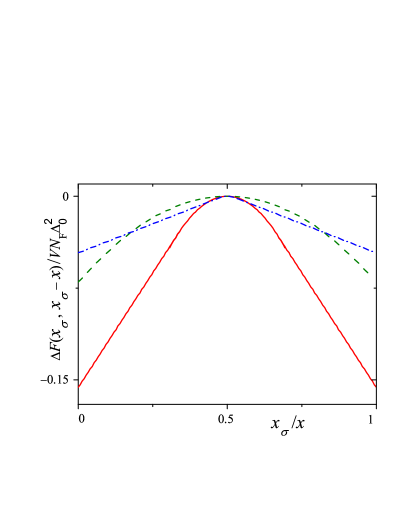
Figure 3: Dependence of $\Delta F=F_{\sigma}(x_{\sigma})+F_{\sigma}(x-x_{\sigma})-2F(x/2)$ on the partial doping $x_{\sigma}$ calculated at $T=0$ and fixed total doping: $x=0.75x_{0}$ [(green) dashed curve], $x=1.5x_{0}$ [(red) solid curve], and $x=1.9x_{0}$ [(blue) dash-dot curve]. The free energy curves for all three doping values have a global maximum at $x_{\sigma}=x/2$, implying that the usual metallic phase is unstable. The free energy is the lowest for either $x_{\sigma}=0$ or $x_{\sigma}=x$: the free energy minimum at $x_{\sigma}=0$ ($x_{\sigma}=x$) represents a half-metallic state with empty (filled) sector $\sigma$ and filled (empty) sector $\bar{\sigma}$.

The above considerations are valid if the doping $x$ is less than $x_{0}$. To investigate the behavior of the system in a wider doping range, we calculate the function

$$\Delta F(x,x_{\sigma})=F_{\sigma}(x_{\sigma})+F_{\sigma}(x-x_{\sigma})-2F_{\sigma}(x/2)\,.$$ (40)

If $x<x_{0}$, the doping in both sectors is less than $x_{0}$. In this case, the free energy $F_{\sigma}(x_{\sigma})$ is determined by Eq. (24) and

$$\frac{\Delta F(x,x_{\sigma})}{V}=\frac{1}{N_{\textrm{F}}}\left[-\frac{x^{2}}{8}+\frac{x_{\sigma}(x-x_{\sigma})}{2}\right].$$ (41)

The corresponding parabolic curve is shown in Fig. 3 for $x=0.75x_{0}$ by a dashed line as a function of the ratio $x_{\sigma}/x$. This function is negative and reaches its minimum when all charge carriers introduced by the doping are concentrated within one sector (that is, when either $x_{\sigma}=0$, or $x_{\sigma}=x$); whereas the maximum of the function $\Delta F(x,x_{\sigma})$ represents the usual SDW state with $x_{\uparrow}=x_{\downarrow}=x/2$. This means that the ground state corresponds to the spin-valley half-metal phase, while the usual SDW phase is unstable, in agreement with the results obtained above.

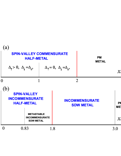
Figure 4: Phase diagram of the system; (a) commensurate and (b) incommensurate ordering. (a) Spin-valley half-metals exist within the doping range $0<x<2x_{0}$. At $x=x_{0}$ (vertical dashed line) order parameter $\Delta_{\uparrow}$ vanishes and a second-order phase transition occurs. However, a characteristic polarization of the charge carriers at the Fermi surface (half-metallicity) is not destroyed. When $x=2x_{0}$ [vertical (red) solid line] a first-order transition occurs from the spin-valley half-metal phase to the PM phase. (b) Spin-valley half-metal exists within the doping range $0<x\lesssim 1.8x_{0}$. At $x\approx 1.8x_{0}$ [(red) solid line] a second-order phase transition occurs from the spin-valley phase to the usual SDW incommensurate state. If $x\approx 3x_{0}$ [vertical thin (black) solid line] a first-order phase transition occurs to the PM phase. The dashed vertical line shows the point ($x\approx 0.83x_{0}$) when the incommensurate SDW order can exist as a metastable phase.

When $x>x_{0}$, the doping in one sector can be larger than $x_{0}$. If $x_{\sigma}>x_{0}$, the order parameter in sector $\sigma$ vanishes, and the partial free energy becomes

$$F_{\sigma}(x_{\sigma})=\frac{x_{\sigma}^{2}}{4N_{\textrm{F}}},$$ (42)

as in the disordered paramagnetic (PM) phase. Thus, for $x>x_{0}$, the function $\Delta F(x,x_{\sigma})$ is a piecewise function with the continuous first (but not second) derivative $\partial\Delta F/\partial x_{\sigma}$. In the vicinity of the point $x_{\sigma}=x/2$, the function $\Delta F$ has a parabolic shape. It coincides with linear functions of $x_{\sigma}$ away from that point, see the (red) solid ($x=1.5x_{0}$) and (blue) dot-dash ($x=1.9x_{0}$) curves in Fig. 3. However, the function $\Delta F(x,x_{\sigma})$ is negative and attains a minimum if either $x_{\sigma}=0$ or $x_{\sigma}=x$. Therefore, the ground state of the model is, again, a spin-valley half-metal. In doing so, we readily obtain that a second order transition occurs at $x=x_{0}$, where the gap in the doped sector is closed. Comparing the free energies of the spin-valley half-metal phase and of the usual PM state, we conclude that the PM state becomes favorable when $x=2x_{0}$. At this point, the gap in the undoped sector closes in a jump-like manner, and a first order transition to the usual PM phase occurs. The obtained results are summarized in Fig. 4(a).

II.2 CDW half-metal

The CDW order is characterized by a finite average value $\langle\hat{\rho}({\bf r})\rangle$ of the density operator

$$\hat{\rho}({\bf r})=\sum_{\sigma{\bf k}}\psi^{\dagger}_{\mathbf{k}a\sigma}\psi^{\phantom{{\dagger}}}_{\mathbf{k}b\sigma}\exp(i{\bf Q}_{0}{\bf r})+{\rm h.c.}$$ (43)

The CDW order is described by a formalism similar to the one developed above for the SDW. To switch between the two types of density waves, the mean-field sectors must be redefined. Specifically, we will assume below that the sector $\sigma$ consists of the operators $\psi_{a\sigma}$ and $\psi_{b\sigma}$. This rearrangement of the sectors may be formally expressed by the substitution

$$\psi_{b\uparrow}\rightarrow\psi_{b\downarrow},\quad\psi_{b{\downarrow}}\rightarrow\psi_{b\uparrow}.$$ (44)

Under this substitution, we have

$$\sum_{{\bf k}\sigma}\langle\psi^{\dagger}_{\mathbf{k}a\sigma}\psi^{\phantom{{\dagger}}}_{\mathbf{k}b\bar{\sigma}}\rangle\rightarrow\sum_{{\bf k}\sigma}\langle\psi^{\dagger}_{\mathbf{k}a\sigma}\psi^{\phantom{{\dagger}}}_{\mathbf{k}b\sigma}\rangle.$$ (45)

Therefore, the finite modulation of the spin density is replaced by a finite modulation of the charge density:

$$2\langle{\hat{S}}^{x}({\bf r})\rangle\rightarrow\langle\hat{\rho}({\bf r})\rangle.$$ (46)

Equation (44) allows us to adopt the results derived for the SDW to describe the CDW state with little modifications.

In the CDW phase, we use the finite expectation values of $\langle\psi^{\dagger}_{\mathbf{k}a\sigma}\psi^{\phantom{{\dagger}}}_{\mathbf{k}b\sigma}\rangle$ and $\langle\psi^{\dagger}_{\mathbf{k}b\sigma}\psi^{\phantom{{\dagger}}}_{\mathbf{k}a\sigma}\rangle$ to apply the mean-field decoupling in Hamiltonians (5) and (6). Unlike the SDW case, both the direct and exchange terms contribute to the mean-field Hamiltonian of the CDW phase:

$$\!\!\!\!\!\!\hat{H}_{\textrm{CDW}}\!\!\! = \!\!\!\!\sum_{\mathbf{k}\sigma\alpha}\!\left[\!\varepsilon^{\alpha}(\mathbf{k})\psi_{\mathbf{k}\alpha\sigma}^{{\dagger}}\psi^{\phantom{{\dagger}}}_{\mathbf{k}\alpha\sigma}\!-\!\tilde{\Delta}^{\vphantom{\dagger}}_{\sigma}\psi^{{\dagger}}_{\mathbf{k}\alpha\sigma}\psi^{\phantom{{\dagger}}}_{\mathbf{k}\bar{\alpha}\sigma}\!+\!\frac{\tilde{\Delta}^{2}_{\sigma}}{\tilde{g}}\!\right]\!\!,$$ (47)

$$\!\!\!\!\!\!\tilde{\Delta}_{\sigma} = \frac{\tilde{g}}{V}\sum_{\mathbf{k}}\left\langle\psi^{\dagger}_{\mathbf{k}a\sigma}\,\psi^{\phantom{{\dagger}}}_{\mathbf{k}b\sigma}\right\rangle\,,$$ (48)

where

$$\tilde{g}=g-2g_{\bot}$$ (49)

is the renormalized electron-electron coupling. Hamiltonian (47) is similar to the SDW Hamiltonian, Eq. (8). Thus, as expected, the CDW problem is mapped onto the SDW one solved in the previous Section. In particular, the CDW order parameter at zero doping is $\tilde{\Delta}_{0}\approx\varepsilon_{\rm F}\exp\left(-1/\tilde{g}N_{\rm F}\right)$. Since $g_{\bot}>0$ (repulsive interaction), the CDW is always either metastable ($\tilde{\Delta}_{0}<\Delta_{0}$), or absolutely unstable ($2g_{\bot}\geq g\Leftrightarrow\tilde{g}<0$). Of course, the stability of the CDW order may be improved by adding parameters, which are beyond our simple model; for example, also considering an applied magnetic field and the interaction with the lattice.

Calculations identical (up to relabeling) to the case of the SDW order demonstrate that for $x>0$ the charge carriers are accumulated in a single mean-field sector. However, the sectors structure is changed by the transformation (44): unlike the case of spin-valley half-metals, now both electronic fields within a single sector have the same spin projection. Therefore, if the introduced charge fills sector $\sigma$, both Fermi surface sheets have identical spin polarizations equal to $\sigma$, see Fig. 2(c). This perfect polarization of the Fermi surface is a hallmark feature of half-metals. Thus, the spin-valley half-metal is related to the CDW half-metal by substitution (44). This substitution, in particular, switches the operators $\hat{S}$ and $\hat{S}_{\rm v}$. Consequently, in the CDW half-metal, we have

$$S=\sigma xV,\quad\text{and}\quad|S_{\rm v}|<|S|,$$ (50)

and $S_{\rm v}=0$ in the case of the perfect electron-hole symmetry. When $x>0$, in addition to the CDW order parameter, the SDW order parameter $\langle\delta S^{z}\rangle$ is generated:

$$\langle\delta S^{z}({\bf r})\rangle=\frac{\tilde{\Delta}_{\uparrow}\!-\!\tilde{\Delta}_{\downarrow}}{g}\cos({\bf Q}_{0}{\bf r}).$$ (51)

It grows monotonically with $x$. This is a direct analog of Eq. (39).

In the case of CDWs, we obtain formulas for the free energy, chemical potential, and order parameter similar to Eqs. (26)–(28), replacing $\Delta_{0}$ by $\tilde{\Delta}_{0}$. Thus, the CDW order parameter is at least metastable in the doping range

$$0<x<2\tilde{x}_{0}=2N_{\textrm{F}}\tilde{\Delta}_{0}.$$ (52)

Since $\tilde{x}_{0}<x_{0}$, the CDW phase becomes absolutely unstable at lower doping value than that in the SDW. To illustrate this, let us now calculate the difference in the free energy between the CDW half-metal and the spin-valley half-metal

$$\frac{\Delta F}{V}=N_{\textrm{F}}\left(\Delta_{0}^{2}-\tilde{\Delta}_{0}^{2}\right)-\left(\Delta_{0}-\tilde{\Delta}_{0}\right)x.$$ (53)

It is easy to see that, as long as $x<\tilde{x}_{0}$ and $\Delta_{0}>\tilde{\Delta}_{0}$, the difference $\Delta F$ decreases when doping grows; however, it is always positive. Thus, we conclude that the spin-valley state is more stable than the CDW half-metal phase.

II.3 Incommensurate ordering

Here we analyze a possible incommensurate ordering in the model under discussion Rice (1970); Rakhmanov et al. (2013). We start with the SDW order. The order parameter $\Delta_{\sigma}$, calculated in the previous sections, couples electrons with unequal momenta. Consequently, in coordinate space, the local spin polarization rotates with wave vector $\mathbf{Q}_{0}$. Typically, the centers of different Fermi surface pockets are located near the high-symmetry points of the Brillouin zone. Therefore, the vector $\mathbf{Q}_{0}$ is related to the underlying lattice structure. Such an order may be called commensurate. Yet, as it has been already mentioned above, we may try to relax the requirement of the commensurability and optimize the energy further by treating the translation vector $\mathbf{Q}_{1}=\mathbf{Q}_{0}+\mathbf{Q}$ as a variational parameter. The new order parameter has the form

$$\Delta_{\sigma}(\mathbf{Q})=\frac{g}{V}\sum_{\mathbf{k}}\left\langle\psi^{\dagger}_{\mathbf{k}a\sigma}\,\psi^{\vphantom{\dagger}}_{\mathbf{k+Q}b\bar{\sigma}}\right\rangle\,,$$ (54)

where, as before, the momentum for electrons in band $\alpha$ is measured from the center of the band $\alpha$. The vector $\mathbf{Q}$ is small,

$$|\mathbf{Q}|\sim\Delta_{0}m/k_{\textrm{F}}\ll|\mathbf{Q}_{0}|.$$ (55)

The order parameter (54) describes the SDW order with a rotating spin polarization. This rotation is characterized by the spatial period $2\pi/|\mathbf{Q}_{0}+\mathbf{Q}|$. This value is unrelated to the underlying lattice and such order is called incommensurate.

To describe the incommensurate state, we calculate the grand potential $\Omega$. In the mean-field approach, $\Omega$ is a sum of grand potentials $\Omega_{\sigma}=\Omega_{\sigma}(x_{\sigma})$. Similar to Eq. (9), the eigenvalues of the mean-field Hamiltonian are

$$\!\!E^{(1,2)}_{\mathbf{k}\sigma}\!=\!\frac{\varepsilon_{\mathbf{k+Q}}\!-\!\varepsilon_{\mathbf{k}}}{2}\!\mp\!\sqrt{\Delta_{\sigma}^{2}(\mathbf{Q})\!+\!\left[\frac{\varepsilon_{\mathbf{k+Q}}\!+\!\varepsilon_{\mathbf{k}}}{2}\right]^{2}}\,.$$ (56)

With this new formula for $E^{(1,2)}_{\mathbf{k}\sigma}$, the expression for the partial grand potentials $\Omega_{\sigma}$, Eq. (11), remains unchanged. We add the minimization condition $\partial\Omega_{\sigma}/\partial Q=0$ to Eqs. (12)–(14) and solve the obtained system numerically as it was described in Ref. Rakhmanov et al., 2013 [see Eqs. (11)–(20) of that paper].

The partial free energy $F_{0}^{\rm ic}(x_{\sigma})$ of a sector with partial doping $x_{\sigma}$ in the incommensurate state is calculated according to Eq. (22). Within the considered mean-field approach, the free energy of the system in the presence of the incommensurate SDW equals

$$F^{\rm ic}(x)=\min_{x_{\uparrow}+x_{\downarrow}=x}\left[F_{0}^{\rm ic}(x_{\uparrow})+F_{0}^{\rm ic}(x_{\downarrow})\right]\,.$$ (57)

The free energy of the system in the ground state is found by its minimization under the condition $x_{\uparrow}+x_{\downarrow}=x$. Our numerical analysis shows that

$$\frac{\partial^{2}F_{0}^{\rm ic}(x_{\sigma})}{\partial x_{\sigma}^{2}}<0,$$ (58)

for $x_{\sigma}$ less than the threshold value $x^{*}\cong 0.83x_{0}$. Since the second derivative of $F_{0}^{\rm ic}$ is negative, the sum $F_{0}^{\rm ic}(x_{\uparrow})+F_{0}^{\rm ic}(x-x_{\uparrow})$ as a function of $x_{\uparrow}\in[0,x]$ is concave at not too large $x$. Consequently, the extremum of the latter sum at $x_{\uparrow}=x/2$ corresponds to a maximum, not a minimum [see Fig. 5]. Therefore, the total free energy is minimized as follows:

$$F^{\rm ic}(x)=F_{0}^{\rm ic}(x)+F_{0}^{\rm ic}(0),\,\,\textrm{at}\,\,x_{\sigma}=x\,\,\textrm{and}\,\,x_{\bar{\sigma}}=0.$$ (59)

Thus, the undoped sector ${\bar{\sigma}}$ remains insulating. All doped charge goes to sector $\sigma$, which becomes metallic, with a well-defined Fermi surface, and we recover the spin-valley half-metal with an incommensurate SDW.

Note that the compressibility of the material has the same sign as the second derivative of its free energy. Hence, the compressibility of the system under study is negative at low doping. This is a rather general feature of models with imperfect nesting, which, in particular, gives rise to the possibility of phase separation in them Gorbatsevich et al. (1992); Sboychakov et al. (2013b, c); Rakhmanov et al. (2013); Igoshev et al. (2010).

If $x_{\sigma}>x^{*}$, then

$$\frac{\partial^{2}F_{0}^{\rm ic}(x_{\sigma})}{\partial x_{\sigma}^{2}}>0,$$ (60)

and the total free energy $F_{0}^{\rm ic}(x_{\sigma})+F_{0}^{\rm ic}(x-x_{\sigma})$ acquires a local minimum at $x_{\uparrow}=x_{\downarrow}=x/2$ (see Fig. 5). When doping increases even further, this minimum becomes a global minimum for $x\cong 1.8N_{F}\Delta_{0}$. Consequently, the first order transition from incommensurate spin-valley half-metal to the usual incommensurate SDW phase occurs at this point.

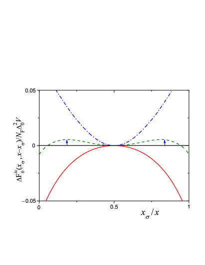
Figure 5: Dependence of $\Delta F_{0}^{\rm ic}(x_{\sigma},x-x_{\sigma})\equiv F_{0}^{\rm ic}(x_{\sigma})+F_{0}^{\rm ic}(x-x_{\sigma})-2F_{0}^{\rm ic}(x/2)$ on the partial doping $x_{\sigma}$, calculated at $T=0$ and fixed total doping $x=1.4x_{0}$ [(red) solid curve], $x=1.76x_{0}$ [(green) dashed curve], and $x=2.0x_{0}$ [(blue) dash-dot curve]. At high doping ($x=2.0x_{0}$), the state at $x_{\sigma}=x_{\bar{\sigma}}=x/2$ has the lowest free energy, therefore, the usual metal, with even distribution of the doped charges among the sectors, is a stable phase. When the doping is low ($x=1.4x_{0}$), the half-metal is stable. In this situation, the free energy minimum at $x_{\sigma}=0$ ($x_{\sigma}=x$) represents a half-metallic state with empty (filled) sector $\sigma$ and filled (empty) sector $\bar{\sigma}$. At some intermediate doping $1.4x_{0}<x^{*}<2.0x_{0}$, a first order transition from the usual metal to the half-metal occurs. Near the transition, one of the phases may become metastable. For example, a well-defined local (but not global) minimum of the free energy at $x_{\sigma}=x_{\bar{\sigma}}=x/2$ is clearly seen for the (green) dashed curve. This implies that for $x=1.76x_{0}$, the usual metal is metastable, while the half-metal is truly stable. The activation barriers for the transition into the more stable half-metallic phase are shown by the vertical arrows. The presence of the metastable phase is marked in Fig. 4(b).

The results obtained are summarized in Fig. 4(b). Comparing them with the case of commensurate order [Fig. 4(a)], we observe a definite difference. While the spin-valley half-metal exists in both cases approximately within the same doping ranges, the transition from the half-metal to the PM phase occurs in a different way: directly from the half-metal to the PM if ${\bf Q}=0$ and via the intermediate incommensurate SDW state if ${\bf Q}\neq 0$.

Comparing the computed free energies of the commensurate and incommensurate phases, we see that the incommensurate phase is more stable than the commensurate one. Accounting for the incommensurability allows us to extend the range of existence for the ordered state, as one can notice comparing Fig. 4(a) and 4(b). However, the difference between the ordering with ${\bf Q}=0$ and ${\bf Q}\neq 0$ is small. The contributions, which are ignored in our treatment (e.g., disorder), can be favorable for commensurate ordering.

The results for the CDW phase can be obtained from the above calculations by a simple replacement ${\Delta}_{0}\rightarrow\tilde{\Delta}_{0}$, and, consequently, the incommensurate CDW half-metal is the ground state of the system at low doping.

Among the four mean-field states discussed here (commensurate SDW/CDW half-metals, incommensurate SDW/CDW half-metals), the incommensurate SDW has the lowest energy at low doping, within the framework of our model. However, the difference in free energy between the SDW and CDW phases may be small. Indeed, the direct interaction parameter $g$ equals to $g(0)$, where $g({\bf k})$ is the Fourier transform of the inter-electron repulsion energy $g({\bf r})$, while the exchange interaction parameter $g_{\bot}$ represents the interaction at the momentum transfer $\mathbf{Q}_{1}\approx\mathbf{Q}_{0}$: $g_{\bot}=g({\bf Q}_{1})$. If $g({\bf Q}_{1})\ll g(0)$ (e.g., as in the case of bare Coulomb repulsion), then, $g_{\bot}\ll g$ and $\Delta\approx\tilde{\Delta}$. Also, other factors, which are not included in our study, could favor the CDW half-metal. For example, the proximity to a lattice instability can make the CDW half-metal a ground state. The applied magnetic field acts similarly, since the total spin of the CDW half-metal exceeds the spin of the spin-valley half-metal.

III Electric, spin, and spin-valley conductivities

In the system under study, the charge carriers at the Fermi surface are spin or spin-valley polarized. Consequently, the currents are also polarized. The problem of the polarized currents in our half-metal deserves a separate investigation and here we only discuss this very briefly. In particular, we assume the perfect electron-hole symmetry and consider only commensurate ordering, since in the case of incommensurate SDW or CDW the results are qualitatively similar.

The electrical conductivity of the isotropic system at zero temperature in the free-electron approximation can be written as Han (2013)

$$\sigma_{\rm E}=\frac{e^{2}}{3}N_{\textrm{F}}(\mu)\,\tau(\mu)\,v^{2}(\mu),$$ (61)

where $N_{\textrm{F}}(\mu)$ is the density of states, $\tau(\mu)$ is the mean free time, and $v(\mu)=|\partial\varepsilon_{\mathbf{k}}/\partial{\bf k}|$ is the electron velocity, and all values here are taken at the Fermi level $\mu$. For simplicity, we assume further that the mean free time is the same for electrons and holes and is independent of $\mu$. In Eq. (61), electrons with both spin projections are taken into account. For a quadratic electron dispersion, we have $\sigma_{\rm E}=e^{2}n\tau/m$, where $n$ is the electron density in the conduction band.

If we neglect the electron-hole coupling, the conductivity of the two-band system, Fig. 1, is the sum of the electron and hole conductivities, $\sigma_{\rm E}=\sigma_{a}+\sigma_{b}$. When doping is zero, we have

$$\sigma_{a}=\sigma_{b}=e^{2}n_{0}\tau/m=\sigma_{0},\quad\text{and thus,}\quad\sigma_{\rm E}=2\sigma_{0}.$$ (62)

Here $n_{0}=k^{3}_{\textrm{F}}/(6\pi^{2})$ is the density of electrons ($n_{a}$) or holes ($n_{b}$) in the conduction band at zero doping. If we dope the system electronically, then, $n_{a}=n_{0}+x$. Assuming that $x\ll n_{0}$, we obtain in the linear approximation: $n_{b}\approx n_{0}-x$. Therefore, the electrical conductivity remains approximately constant, $\sigma_{\textrm{E}}(x)\approx 2\sigma_{0}$. In this framework, the Fermi surface is spin degenerate; consequently, the corresponding spin conductivity is zero.

III.1 Spin-valley half-metal

First, we consider the case of SDW instability and spin-valley half-metal. The electron-hole coupling opens a gap in the spectrum and the conductivity in the system becomes equal to zero at zero doping.

At finite doping, the mobile charge carriers are accumulated in the conduction bands. When $x<x_{0}$, the band corresponding to the sector $\sigma=+1/2$ is filled, while the band corresponding to $\sigma=-1/2$ is empty. We have two Fermi-pockets in the filled band, one electron-like ($\partial E_{\mathbf{k}}/\partial k>0$) and one hole-like, ($\partial E_{\mathbf{k}}/\partial k<0$), see Fig. 2. The Fermi momenta of these pockets are given by Eq. (30), where $\mu=E_{\mathbf{k}\sigma}$. Using Eqs. (18) and having in mind that $\Delta/\varepsilon_{\textrm{F}}\ll 1$, we derive

$$\frac{k_{\rm F}^{(e,h)}}{k_{\rm F}}=1\pm\frac{\Delta_{0}}{4\varepsilon_{\rm F}}\frac{x}{x_{0}}\approx 1,\quad x<x_{0},$$ (63)

where the superscript $e$ (superscript $h$) and the plus (minus) sign corresponds to the electron (hole) pocket. Recall that $k_{\rm F}$ and $\varepsilon_{\rm F}$ denote the corresponding values at zero doping. In the same approximation, we have

$$v_{F}^{(e,h)}\!\!\approx\!\pm\frac{x}{2x_{0}\!-\!x}\frac{k_{F}}{m},\,\,N_{F}^{(e,h)}\!\!\approx\!\frac{2x_{0}\!-\!x}{x}N_{F},\,\,x<x_{0}.$$ (64)

Therefore, in the lowest-order approximation, when $\Delta_{0}/\varepsilon_{F}\ll 1$, the electron-hole symmetry is preserved.

The energy gap $\Delta_{\sigma}$ in the $\sigma=+1/2$ sector vanishes if $x>x_{0}$, while the filling of the $\sigma=-1/2$ sector remains zero (see Section II.1). Thus, for $\Delta_{0}/\varepsilon_{\textrm{F}}\ll 1$, the conductivity becomes $\sigma_{0}$, that is, one-half of the conductivity of the system in the PM state.

Now we can calculate the electric conductivity $\sigma_{\textrm{E}}$, which is the sum of the electron, $\sigma_{e}$, and the hole, $\sigma_{h}$, contributions. Using Eq. (61) and (64), we obtain

$$\sigma_{\textrm{E}}=\sigma_{0}G(x)\approx\sigma_{0}\!\left\{\!\begin{array}[]{ll}x/(2x_{0}-x),&\hbox{$0<x<x_{0}$,}\\ 1,&\hbox{$x_{0}<x<2x_{0}$.}\end{array}\right.$$ (67)

The derivative of the function $\sigma_{\textrm{E}}(x)$ has a singularity at $x=x_{0}$, when the second order transition occurs [see Fig. 4(a)]. When $x>2x_{0}$, the half-metal phase disappears, the spin degeneracy of the Fermi surface is restored, and the conductivity exhibits a stepwise change from $\sigma\approx\sigma_{0}$ to $\sigma\approx 2\sigma_{0}$.

The conductivity in the half-metallic state is of the order of $\sigma_{0}$ if the doping $x$ is not small, $x\sim x_{0}$. The results obtained are valid if the temperature $T$ and scattering frequency $1/\tau$ are both smaller than the characteristic energy $\mu-\Delta_{\sigma}$, which is necessary “to mix” the electrons-like and the hole-like excitations. When $x\sim x_{0}$, this means that both $T,1/\tau\ll\Delta_{0}$.

If the electric current $j$ is spin-polarized, the spin current $j^{s}$ associated with $j$ is nonzero. We can define the spin current as $j^{s}=j\langle s_{z}\rangle/e$, where $\langle s_{z}\rangle$ is the average spin projection per one electron or hole at the Fermi surface. Using Eq. (61), we define a spin conductivity as

$$\sigma^{s}=\frac{e\langle s_{z}\rangle}{3}\,N_{\textrm{F}}(\mu)\,\tau(\mu)\,v^{2}(\mu),$$ (68)

where we assume that there are no magnetic impurities in the sample. The spin conductivity of the system is the sum of spin conductivities in the electron $\sigma_{e}^{s}$, and the hole, $\sigma_{h}^{s}$ pockets. To calculate $\sigma^{s}$, we need to know the spin polarization of the Fermi surface valleys. At small doping $x\ll x_{0}$, the valley polarizations are weak $|\langle s_{z}\rangle|\ll 1/2$. They grow as the doping increases, and saturate when $x\thicksim x_{0}$. In this case, we have $\langle s_{z}\rangle\approx 1/2$ for the electrons and $\langle s_{z}\rangle\approx-1/2$ for holes. Therefore, $\sigma_{e}^{s}\approx-\sigma_{h}^{s}$, and

$$\sigma^{s}\approx 0$$ (69)

with an accuracy $\sim\sigma^{s}_{0}(\Delta_{0}/\varepsilon_{\rm F})$, where $\sigma^{s}_{0}=\sigma_{0}/2e$.

In our system, we can define the spin-valley conductivity as well. Indeed, similarly to the electron spin, we can attribute the spin-valley quantum number $\pm 1/2$ to the electron states at the Fermi energy, see Eq. (33). When the electrical current flows through the system, it can carry this quantum number, in addition to the charge.

To specify the spin-valley conductivity, we replace the spin polarization $\langle s_{z}\rangle$ in Eq. (68) by an average spin-valley projection $\langle s_{v}\rangle$. For the spin-valley half-metal, $\langle s_{v}\rangle=1/2$ for both Fermi pockets. As a result, we readily obtain

$$\sigma^{v}=\sigma_{0}^{v}G(x),$$ (70)

where $\sigma_{0}^{v}=\sigma_{0}^{s}=\sigma_{0}/2e$.

III.2 CDW half-metal

In the case of the CDW half-metal, electron-like and hole-like charge carriers have the same spin projections, while the spin-valley projections have opposite signs. It is easily proven that in the CDW case, the charge conductivity is the same as for the SDW phase, Eq. (67), while the spin and spin-valley conductivities must be interchanged, as compared to the spin-valley half-metal phase, that is,

$$\sigma_{\textrm{E}}\!=\!\sigma_{0}G(x),\quad\sigma^{s}\!=\!\sigma_{0}^{s}G(x),\quad\sigma^{v}\!\approx\!0.$$ (71)

We can see from Eqs. (71) and (70) that the electric current in our systems carries, besides charge, an additional quantum number: either spin, or spin-valley projection.

IV Superconductivity

In the half-metal phases under study, we have itinerant electrons in two Fermi pockets. Therefore, an attractive interaction between these quasiparticles can give rise to unconventional superconductivity. We briefly analyze such a possibility. For simplicity, we consider below only commensurate SDW or CDW ordering.

Let us assume that the effective Hamiltonian of the system can be written as

$$\hat{H}_{\textrm{eff}}=\hat{H}_{\textrm{HM}}+\hat{H}_{\textrm{{BCS}}},$$ (72)

where the first term in the right-hand side, $\hat{H}_{\textrm{HM}}$, corresponds either to the spin-valley SDW phase, Eq. (8), or to the CDW half-metal, Eq. (47). The second term is a usual BCS attraction. We consider first the CDW phase. In this case, all electrons in both Fermi-pockets have the same spin projection $\sigma=\uparrow$. Thus, the BCS term can be expressed as

$$\hat{H}_{\textrm{BCS}}=-\!\!\sum_{\mathbf{kk}^{\prime}\alpha\beta}\!{V^{\alpha\beta}_{\mathbf{kk^{\prime}}}C^{\dagger}_{\mathbf{k}\uparrow\alpha}C^{\dagger}_{\mathbf{-k}\uparrow\alpha}C_{\mathbf{-k^{\prime}}\uparrow\beta}C_{\mathbf{k^{\prime}}\uparrow\beta}}\,,$$ (73)

where $C^{\dagger}_{\mathbf{k}\uparrow\alpha}$ ($C_{\mathbf{k}\uparrow\alpha}$) are the creation (annihilation) operators of a quasiparticle with momentum $\mathbf{k}$ and spin projection $\uparrow$ at the Fermi surface pocket $\alpha=e,h$; while $V^{\alpha\beta}_{\mathbf{kk^{\prime}}}=V^{\beta\alpha}_{\mathbf{kk^{\prime}}}$ are the corresponding matrix elements of the electron-electron attraction.

The superconducting order parameter is commonly defined as

$$\Delta_{\rm sc}^{\alpha}(\mathbf{k})=\sum_{\mathbf{k}^{\prime}\beta}{V^{\alpha\beta}_{\mathbf{kk}^{\prime}}}\left\langle C^{\dagger}_{\mathbf{k^{\prime}}\uparrow\beta}C^{\dagger}_{\mathbf{-k^{\prime}}\uparrow\beta}\right\rangle.$$ (74)

In particular, this means that

$$\Delta_{\rm sc}^{\alpha}(\mathbf{k})=-\Delta_{\rm sc}^{\alpha}(-\mathbf{k})\,.$$ (75)

Following the standard Bogolyubov approach for the case of two-band superconductivity Suhl et al. (1959), we obtain a system of equations for calculating the two superconducting gaps

$$\Delta_{\rm sc}^{\alpha}(\mathbf{k})=-\sum_{\mathbf{k}^{\prime}\beta}{\frac{V^{\alpha\beta}_{\mathbf{kk}^{\prime}}\Delta_{\rm sc}^{\beta}(\mathbf{k^{\prime}})}{2E^{\beta}_{\mathbf{k^{\prime}}}}}\tanh{\!\!\left(\frac{E^{\beta}_{\mathbf{k^{\prime}}}}{2T}\right)},$$ (76)

where

$$E^{\alpha}_{\mathbf{k}}=\sqrt{\left(E^{(2)}_{\mathbf{k}\uparrow}-\mu\right)^{2}+\Delta_{\rm sc}^{\alpha}(\mathbf{k})^{2}}\,.$$ (77)

In this expression $E^{(2)}_{\mathbf{k}\uparrow}$ is determined by Eq. (9), in which the SDW order parameter $\Delta_{\sigma}$ should be replaced by the CDW order parameter $\tilde{\Delta}_{\sigma}$. Note that in the case of the CDW half-metal, both gaps $\Delta_{\rm sc}^{e,h}(\mathbf{k})$ correspond to superconductivity with a spin-polarized supercurrent.

In the case of a usual half-metal, an unconventional superconducting ordering exists if the matrix element of the electron-electron attraction obeys certain symmetry rules Pickett (1996); Rudd and Pickett (1998). In contrast to a usual half-metal, we have a two-component superconducting order parameter, one component per one valley. However, the symmetry analysis of $V^{\alpha\beta}_{\mathbf{kk}^{\prime}}$ is very similar to the case of a single-component unconventional superconductivity. We simply have to demand that the symmetry of the matrix element should be consistent with the symmetry of the order parameters, Eq. (75).

For simplicity, let us assume that $V^{ee}_{\mathbf{kk}^{\prime}}=V^{hh}_{\mathbf{kk}^{\prime}}=V^{eh}_{\mathbf{kk}^{\prime}}=V_{\mathbf{kk}^{\prime}}$. These assumptions are reasonable, since the difference in the Fermi momenta of different Fermi pockets is small. From the definition

$$V_{\mathbf{kk}^{\prime}}=\langle\mathbf{k}^{\prime}\uparrow,-\mathbf{k}^{\prime}\uparrow|V|\mathbf{k}\uparrow,-\mathbf{k}\uparrow\rangle.$$ (78)

Thus, the matrix element must obey the following symmetry rules Sigrist and Ueda (1991); Rudd and Pickett (1998)

$$V_{\mathbf{kk}^{\prime}}=-V_{\mathbf{-kk}^{\prime}}=-V_{\mathbf{k-k}^{\prime}}=V_{\mathbf{-k-k}^{\prime}}.$$ (79)

We conclude that the interaction matrix element should have a definite $\mathbf{k}$-space dependence, otherwise $V_{\mathbf{kk}^{\prime}}=0$ according to Eq. (79) and then superconductivity would be impossible. This non-trivial $\mathbf{k}$-space dependent interaction must ensure a correct sign of the sum in the right-hand side of Eq. (76). For example, if the matrix element has the form

$$V_{\mathbf{kk}^{\prime}}=-\frac{\mathbf{kk}^{\prime}}{k_{F}^{2}}V_{0},$$ (80)

then $V_{0}$ must be positive and

$$\Delta_{\rm sc}^{\alpha}(\mathbf{k})=f(\mathbf{k})\bar{\Delta}_{\rm sc}^{\alpha}.$$ (81)

Here $\bar{\Delta}_{\rm sc}^{\alpha}$ is $\mathbf{k}$-independent and derived as the usual BCS superconducting gap in the case of the two-band model Suhl et al. (1959). It depends on the Fermi momenta $k_{F}^{\alpha}$ defined by Eq. (63) and on the interaction parameter $V_{0}$.

The above discussion can be easily adopted to the case of the spin-valley half-metal phase. The only difference is that the spin polarizations of the two valleys are antiparallel to each other. Consequently, the supercurrent carries a spin-valley polarization. As for the spin polarization of the current, it is small, or even zero.

As in the case of the usual BCS treatment, our consideration of the superconductivity is valid if the superconducting gap is much smaller than the characteristic Fermi energy of the half-metal state. That is,

$$|\bar{\Delta}_{\rm sc}^{\alpha}|\ll\Delta_{0}(1-x/2x_{0}-\sqrt{1-x/x_{0}}),$$ (82)

which in the case of sufficiently high doping, $x\sim x_{0}$, reduces to the condition $|\bar{\Delta}_{\rm sc}^{\alpha}|\ll\Delta_{0}$.

V Discussion

Here we have discussed a weak-coupling mechanism of half-metallicity. Since it does not require a strong electron-electron coupling, it may be operational in systems composed of light atoms only. For example, the proposed half-metallicity could exist in systems without transition metals. Moreover, in addition to the usual half-metal with spin-polarized electrons at the Fermi surface, we predicted the possible existence of a new phase, which we referred to as a spin-valley half-metal. This phase is characterized by the valley quantum number, and the charge carriers at the Fermi surface are not only spin-polarized but also valley-polarized. This unique property may be of interest for applications in spintronics, and the newly emerging field of spin-valley-tronics.

The presented mechanism for the formation of half-metallicity is quite general, and may be relevant to any material with nesting-driven density waves. However, here we consider only a specific type of interaction, namely, short-range electron-electron repulsion, Eqs. (4)–(6), with $g$ and $g_{\bot}>0$. In this case, we observe two instabilities of the electronic state: SDW and CDW. From the former, the spin-valley half-metal state emerges, Fig. 2(b), while the latter one gives rise to the CDW half-metal state, Fig. 2(c). Note that in real materials, a short-range approximation for the electron-electron coupling is well justified when the system is in a metallic (or in our case half-metallic) state. In the SDW or CDW insulating state, the long-range interaction could be of significance. However, the use of a more sophisticated interaction potential does not affect our main results: the density-wave instability occurs in the system with nesting under the condition of weak coupling and the ground state of doped system (when the electron-electron interaction is a short-range one) is the half-metal.

We assume that both the electron and hole sheets of the Fermi surface are perfectly nested at zero doping. More realistically, the sheets have non-identical shapes, causing finite denesting even at zero doping. For example, one sheet may be spherical, while the other may be elliptical Sboychakov et al. (2013c).

If the zero-doping denesting is sufficiently weak, the range of doping where $\partial^{2}F^{\rm ic}_{0}(x)/\partial x^{2}<0$ shrinks Sboychakov et al. (2013c), but does not disappear. When the sheet shapes differ significantly, one has $\partial^{2}F^{\rm ic}_{0}(x)/\partial x^{2}>0$ for all $x$, and the half-metallic states become impossible.

On the other hand, if the sheets are non-spherical, but the zero-doping nesting is preserved (at $x=0$ the sheets are identical), our conclusions endure, and only minor mathematical modifications to the formalism are required (the density of states acquires a dependence on the spherical angles).

In addition, we assumed the electron-hole symmetry of the “bare” (when the electron-hole coupling is neglected) bands, Fig. 1. This approximation simplifies the intermediate formulas considerably; fortunately, it does not trivialize the main results. Straightforward modifications to the formalism allows one to study a more general model.

It is interesting to note that the model we investigate in this paper is well-known and was discussed in many research papers. Yet, despite these efforts, Hamiltonian (3) provides an unexpected many-body phase of electronic liquid. This is associated with the fact that a doped density-wave system has several states whose energies are almost identical (“stripes”, phase separation, incommensurate density waves). They compete against each other to become the “true” ground state. The multiplicity of the competing phases makes a theoretical description particularly challenging: it is impossible to prove that no new states will not be added to the list in the future. Thus, to realize the proposed mechanism in an actual material, a multidisciplinary study is necessary. In addition to analytical many-body tools, numerical ab initio calculations of Fermi surfaces and other electronic and lattice properties are highly desirable. Of course, a guidance from the experiment is indispensable in such a study.

The most striking feature of the half-metal states considered in this paper is the possibility to observe spin or spin-valley polarized currents. The corresponding conductivities are significant if the doping is not small and is of the order of the characteristic value

$$x_{0}=N_{\textrm{F}}\Delta_{0}\sim\Delta_{0}n_{0}/\varepsilon_{\textrm{F}}.$$ (83)

In this regime, the results obtained are valid at sufficiently low temperatures, $T\ll\Delta_{0}$, and in the absence of a strong electron scattering, $1/\tau\ll\Delta_{0}$. The absence of magnetic impurities that spoil the spin polarization is also necessary. We neglected here several perturbations (disorder, spin-orbit coupling, Umklapp processes). The stability margins of the half-metallic phases against these factors, as well as their effects on the polarized currents, should be checked in further studies.

Since the half-metals posses an ungapped Fermi surface, superconductivity may coexist with these phases. The allowed type of superconductivity is $p$-wave, with parallel or antiparallel orientations of spin polarizations on the electronic and hole sheets. When the polarizations are parallel (antiparallel), the supercurrent, in addition to the electric charge, carries also spin (spin-valley) quantum.

The electronic phase separation and formation of inhomogeneous states of electronic matter is an inherent property of systems with imperfect nesting Rakhmanov et al. (2013, 2017). A strong long-range Coulomb repulsion suppresses the formation of inhomogeneous states. We assumed that this Coulomb interaction guarantees the homogeneity of the electron liquid and neglected the possibility of phase separation. However, the problem of phase separation in the system considered here is of interest and deserves a separate analysis because it makes the phase diagram of the model richer.

The above calculations demonstrate that, among several mean-field states discussed above, the incommensurate spin-valley half-metal has the lowest energy, at least for not too strong doping. However, in realistic $sp$-electron materials the exchange interaction is small sp_exchange . Then, the renormalization of the interaction constant for the CDW ordering Eq. (49) is also small. Therefore, the difference in the free energies between the SDW and CDW phases cannot be large. The difference in the free energy between the incommensurate and commensurate states is also small if coupling is weak, as it follows directly from our calculations. It is reasonable to assume that, in general, factors neglected in our treatment (temperature, magnetic field, disorder, electron-lattice coupling, etc.) may change the ground state. However, in any of the studied half-metal phases, one can observe either spin or spin-valley currents.

To conclude, we discussed the recently proposed weak-coupling mechanism for half-metallicity, as well as its most immediate consequences. We calculated the phase diagram for the studied model and explored the connection between spin conductivity, spin-valley conductivity, and usual electric conductivity for different phases of the model. We also pointed out that in our model the half-metallicity may coexist with superconductivity. The supercurrent in such a superconducting phase would demonstrate nontrivial spin or spin-valley polarization. The mechanism discussed in this work may be of importance for the current search for non-toxic biologically-compatible materials with nontrivial electronic properties.

References

- de Groot et al. (1983) R. A. de Groot, F. M. Mueller, P. G. van Engen, and K. H. J. Buschow, “New Class of Materials: Half-Metallic Ferromagnets,” Phys. Rev. Lett. 50, 2024 (1983).
- Katsnelson et al. (2008) M. I. Katsnelson, V. Y. Irkhin, L. Chioncel, A. I. Lichtenstein, and R. A. de Groot, “Half-metallic ferromagnets: From band structure to many-body effects,” Rev. Mod. Phys. 80, 315 (2008).
- Hu (2012) X. Hu, “Half-Metallic Antiferromagnet as a Prospective Material for Spintronics,” Adv. Mater. 24, 294 (2012).
- Žutić et al. (2004) I. Žutić, J. Fabian, and S. Das Sarma, “Spintronics: Fundamentals and applications,” Rev. Mod. Phys. 76, 323 (2004).
- Hanssen et al. (1990) K. E. H. M. Hanssen, P. E. Mijnarends, L. P. L. M. Rabou, and K. H. J. Buschow, “Positron-annihilation study of the half-metallic ferromagnet NiMnSb: Experiment,” Phys. Rev. B 42, 1533 (1990).
- Park et al. (1998) J.-H. Park, E. Vescovo, H.-J. Kim, C. Kwon, R. Ramesh, and T. Venkatesan, “Direct evidence for a half-metallic ferromagnet,” Nature 392, 794 (1998).
- Ji et al. (2001) Y. Ji, G. J. Strijkers, F. Y. Yang, C. L. Chien, J. M. Byers, A. Anguelouch, G. Xiao, and A. Gupta, “Determination of the Spin Polarization of Half-Metallic by Point Contact Andreev Reflection,” Phys. Rev. Lett. 86, 5585 (2001).
- Jourdan et al. (2014) M. Jourdan, J. Miná r, J. Braun, A. Kronenberg, S. Chadov, B. Balke, A. Gloskovskii, M. Kolbe, H. Elmers, G. Schönhense, et al., “Direct observation of half-metallicity in the Heusler compound Co2MnSi,” Nat. Commun. 5, 3974 (2014).
- (9) M. P. Ghimire, L.-H. Wu, and Xiao Hu, ”Possible half-metallic antiferromagnetism in an iridium double-perovskite material”, Phys. Rev. B 93, 134421 (2016).
- Du et al. (2012) A. Du, S. Sanvito, and S. C. Smith, “First-Principles Prediction of Metal-Free Magnetism and Intrinsic Half-Metallicity in Graphitic Carbon Nitride,” Phys. Rev. Lett. 108, 197207 (2012).
- Hashmi and Hong (2014) A. Hashmi and J. Hong, “Metal free half metallicity in 2D system: structural and magnetic properties of g-C4N3 on BN,” Sci. Rep. 4, 4374 (2014).
- Son et al. (2006) Y.-W. Son, M. L. Cohen, and S. G. Louie, “Half-metallic graphene nanoribbons,” Nature 444, 347 (2006).
- Kan et al. (2012) E. Kan, W. Hu, C. Xiao, R. Lu, K. Deng, J. Yang, and H. Su, “Half-metallicity in organic single porous sheets,” Journal of the American Chemical Society 134, 5718 (2012).
- Huang et al. (2010) B. Huang, C. Si, H. Lee, L. Zhao, J. Wu, B.-L. Gu, and W. Duan, “Intrinsic half-metallic BN–C nanotubes,” Applied Physics Letters 97, 043115 (2010).
- Soriano and Fernández-Rossier (2010) D. Soriano and J. Fernández-Rossier, “Spontaneous persistent currents in a quantum spin Hall insulator,” Phys. Rev. B 82, 161302 (2010).
- Klauk (2010) H. Klauk, “Organic thin-film transistors,” Chem. Soc. Rev. 39, 2643 (2010).
- Avouris et al. (2007) P. Avouris, Z. Chen, and V. Perebeinos, “Carbon-based electronics,” Nat. Nanotechnol. 2, 605 (2007).
- Rozhkov et al. (2011) A. Rozhkov, G. Giavaras, Y. P. Bliokh, V. Freilikher, and F. Nori, “Electronic properties of mesoscopic graphene structures: Charge confinement and control of spin and charge transport,” Phys. Rep. 503, 77 (2011).
- Sa-Ke et al. (2014) W. Sa-Ke, T. Hong-Yu, Y. Yong-Hong, and W. Jun, “Spin and valley half metal induced by staggered potential and magnetization in silicene,” Chin. Phys. B 23, 017203 (2014).
- Rozhkov et al. (2016) A. Rozhkov, A. Sboychakov, A. Rakhmanov, and F. Nori, “Electronic properties of graphene-based bilayer systems,” Phys. Rep. 648, 1 (2016).
- Rozhkov et al. (2017) A. V. Rozhkov, A. L. Rakhmanov, A. O. Sboychakov, K. I. Kugel, and F. Nori, “Spin-Valley Half-Metal as a Prospective Material for Spin Valleytronics,” Phys. Rev. Lett. 119, 107601 (2017).
- Rice (1970) T. M. Rice, “Band-Structure Effects in Itinerant Antiferromagnetism,” Phys. Rev. B 2, 3619 (1970).
- Rakhmanov et al. (2013) A. L. Rakhmanov, A. V. Rozhkov, A. O. Sboychakov, and F. Nori, “Phase separation of antiferromagnetic ground states in systems with imperfect nesting,” Phys. Rev. B 87, 075128 (2013).
- Gorbatsevich et al. (1992) A. Gorbatsevich, Y. Kopaev, and I. Tokatly, “Band theory of phase stratification,” Zh. Eksp. Teor. Fiz. 101, 971 (1992), [Sov. Phys. JETP 74, 521 (1992)].
- Eremin and Chubukov (2010) I. Eremin and A. V. Chubukov, “Magnetic degeneracy and hidden metallicity of the spin-density-wave state in ferropnictides,” Phys. Rev. B 81, 024511 (2010).
- Rakhmanov et al. (2012) A. L. Rakhmanov, A. V. Rozhkov, A. O. Sboychakov, and F. Nori, “Instabilities of the -Stacked Graphene Bilayer,” Phys. Rev. Lett. 109, 206801 (2012).
- Sboychakov et al. (2013a) A. O. Sboychakov, A. V. Rozhkov, A. L. Rakhmanov, and F. Nori, “Antiferromagnetic states and phase separation in doped -stacked graphene bilayers,” Phys. Rev. B 88, 045409 (2013a).
- Sboychakov et al. (2013b) A. O. Sboychakov, A. L. Rakhmanov, A. V. Rozhkov, and F. Nori, “Metal-insulator transition and phase separation in doped -stacked graphene bilayer,” Phys. Rev. B 87, 121401 (2013b).
- Sboychakov et al. (2013c) A. O. Sboychakov, A. V. Rozhkov, K. I. Kugel, A. L. Rakhmanov, and F. Nori, “Electronic phase separation in iron pnictides,” Phys. Rev. B 88, 195142 (2013c).
- Akzyanov et al. (2014) R. S. Akzyanov, A. O. Sboychakov, A. V. Rozhkov, A. L. Rakhmanov, and F. Nori, “-stacked bilayer graphene in an applied electric field: Tunable antiferromagnetism and coexisting exciton order parameter,” Phys. Rev. B 90, 155415 (2014).
- Sboychakov et al. (2017) A. O. Sboychakov, A. L. Rakhmanov, K. I. Kugel, A. V. Rozhkov, and F. Nori, “Magnetic field effects in electron systems with imperfect nesting,” Phys. Rev. B 95, 014203 (2017).
- Moreo et al. (1999) A. Moreo, S. Yunoki, and E. Dagotto, “Phase Separation Scenario for Manganese Oxides and Related Materials,” Science 283, 2034 (1999).
- Dagotto (2003) E. Dagotto, Nanoscale Phase Separation and Colossal Magnetoresistance, Springer Series in Solid-State Sciences (Springer, Berlin, 2003).
- Dagotto et al. (2003) E. Dagotto, J. Burgy, and A. Moreo, “Nanoscale phase separation in colossal magnetoresistance materials: lessons for the cuprates?,” Solid State Commun. 126, 9 (2003), proceedings of the High-Tc Superconductivity Workshop.
- Igoshev et al. (2010) P. A. Igoshev, M. A. Timirgazin, A. A. Katanin, A. K. Arzhnikov, and V. Y. Irkhin, “Incommensurate magnetic order and phase separation in the two-dimensional Hubbard model with nearest- and next-nearest-neighbor hopping,” Phys. Rev. B 81, 094407 (2010).
- Lorenzana et al. (2001) J. Lorenzana, C. Castellani, and C. Di Castro, “Phase separation frustrated by the long-range Coulomb interaction. I. Theory,” Phys. Rev. B 64, 235127 (2001).
- Bianconi et al. (2015) A. Bianconi, N. Poccia, A. Sboychakov, A. Rakhmanov, and K. Kugel, “Intrinsic arrested nanoscale phase separation near a topological Lifshitz transition in strongly correlated two-band metals,” Supercond. Sci. Technol. 28, 024005 (2015).
- Han (2013) F. Han, A Modern Course in the Quantum Theory of Solids (World Scientific, 2013), ISBN 9789814417143.
- Suhl et al. (1959) H. Suhl, B. T. Matthias, and L. R. Walker, “Bardeen-Cooper-Schrieffer Theory of Superconductivity in the Case of Overlapping Bands,” Phys. Rev. Lett. 3, 552 (1959).
- Pickett (1996) W. E. Pickett, “Single Spin Superconductivity,” Phys. Rev. Lett. 77, 3185 (1996).
- Rudd and Pickett (1998) R. E. Rudd and W. E. Pickett, “Single-spin superconductivity: Formulation and Ginzburg-Landau theory,” Phys. Rev. B 57, 557 (1998).
- Sigrist and Ueda (1991) M. Sigrist and K. Ueda, “Phenomenological theory of unconventional superconductivity,” Rev. Mod. Phys. 63, 239 (1991).
- Rakhmanov et al. (2017) A. L. Rakhmanov, K. I. Kugel, M. Y. Kagan, A. V. Rozhkov, and A. O. Sboychakov, “Inhomogeneous electron states in the systems with imperfect nesting,” JETP Letters 105, 806 (2017).
- (44) E. Şaşoglu, I. Galanakis, C. Friedrich, S. Blügel, ”Ab initio calculation of the effective on-site Coulomb interaction parameters for half-metallic magnets,” Phys. Rev. B 88, 134402 (2013).