MOCCA-SURVEY database I. Accreting white dwarf binary systems in globular clusters – IV. cataclysmic variables – properties of bright and faint populations

Abstract

We investigate here populations of cataclysmic variables (CVs) in a set of 288 globular cluster (GC) models evolved with the mocca code. This is by far the largest sample of GC models ever analysed with respect to CVs. Contrary to what has been argued for a long time, we found that dynamical destruction of primordial CV progenitors is much stronger in GCs than dynamical formation of CVs, and that dynamically formed CVs and CVs formed under no/weak influence of dynamics have similar white dwarf mass distributions. In addition, we found that, on average, the detectable CV population is predominantly composed of CVs formed via typical common envelope phase (CEP) ($\gtrsim$ 70 per cent), that only $\approx$ 2–4 per cent of all CVs in a GC is likely to be detectable, and that core-collapsed models tend to have higher fractions of bright CVs than non-core-collapsed ones. We also consistently show, for the first time, that the properties of bright and faint CVs can be understood by means of the pre-CV and CV formation rates, their properties at their formation times and cluster half-mass relaxation times. Finally, we show that models following the initial binary population proposed by Kroupa and set with low CEP efficiency better reproduce the observed amount of CVs and CV candidates in NGC 6397, NGC 6752 and 47 Tuc. To progress with comparisons, the essential next step is to properly characterize the candidates as CVs (e.g. by obtaining orbital periods and mass ratios).

1 Introduction

Cataclysmic variables (CVs) are interacting binaries composed of a white dwarf (WD) undergoing dynamically and thermally stable mass transfer from a low-mass companion, usually a main sequence (MS) star (e.g. Warner, 1995; Knigge et al., 2011). They are expected to exist in non-negligible numbers in globular clusters (GCs), which are natural laboratories for testing theories of stellar dynamics and evolution (e.g. Knigge, 2012, for a review on CVs in GCs).

Due to the high stellar crowding in GCs and their intrinsic faintness, CVs are difficult to identify in such environments. Therefore, space telescopes with high spatial resolution and sensitivity such as the Hubble Space Telescope (HST) and the Chandra X-ray Observatory are required to detect them. Until now the best studied GCs with respect to CV populations are NGC 6397 (Cohn et al., 2010), NGC 6752 (Lugger et al., 2017), $\omega$ Cen (Cool et al., 2013) and 47 Tuc (Rivera Sandoval et al., 2018). The identification of CVs in these GCs has been carried out by identifying HST optical counterparts to Chandra X-ray sources. Usually these counterparts show an H$\alpha$ excess (suggesting the presence of an accretion disc), they are bluer than the MS stars and several also show photometric variability in different bands.

In the core-collapsed clusters NGC 6397 and NGC 6752, Cohn et al. (2010) and Lugger et al. (2017) found the CVs to be divided into two populations, a bright and a faint one. On their optical colour-magnitude diagrams (CMDs), bright CVs lie close to the MS and faint CVs close to the WD cooling sequence, being R $\approx$ 21.5 mag the cut-off between both populations. Interestingly, in the non-core-collapsed clusters 47 Tuc and $\omega$ Cen, only one CV population is observed, and is mainly composed of faint CVs.

Another interesting distinction between bright and faint CVs in core-collapsed GCs is related to the level of mass segregation, which is intrinsically connected with the GC relaxation time (proxy for the GC dynamical age) and the CV masses. For core-collapsed GCs, bright CVs are more centrally concentrated than faint CVs, and faint CVs have similar radial distribution to MS turn-off point (MSTO) stars. This result indicates that bright CVs are more massive than faint ones. Also, bright CVs have more massive donors since CVs close to the MS have their fluxes clearly dominated by the donor, which is usually the case for CVs close or above the period gap. Faint CV fluxes are otherwise dominated by the WD and/or accretion disc, which is associated with CVs close to the period minimum, i.e. WZ Sge-type progenitors. Indeed, Cohn et al. (2010) and Lugger et al. (2017) inferred the total mass range for the bright CVs and faint CVs to be $1.5\pm 0.2$ and $0.8\pm 0.2$ M_⊙, respectively. This is consistent with typical WD masses in CVs ($\sim 0.6-1.0$ M_⊙, Zorotovic et al., 2011) and donor masses of $\sim 0.6$ and $\lesssim 0.1$ M_⊙, for bright and faint CVs, respectively.

The case of 47 Tuc is extremely interesting. Even though the CVs in this cluster are predominantly faint, all of them are more centrally concentrated than MSTO stars. The optical fluxes are indicatives of the donor mass, as we already discussed, which implies then that most CVs in 47 Tuc have low-mass donors. This brings then that the CV masses are dominantly the WD masses. Rivera Sandoval et al. (2018) inferred CV masses of $1.4\pm 0.2$ M_⊙ for both bright and faint CVs in 47 Tuc, which is similar to what has been found for bright CVs in NGC 6397 and NGC 6752. However, this implies that, for the faint CVs, the inferred WD masses in 47 Tuc are $\sim 1.2$ M_⊙, which is much higher than the standard WD mass in CVs. These authors explain these high WD masses as the consequence of either a net mass growth (due to an interplay between accretion and nova outbursts) or to X-ray selection effects, since the larger the WD mass (and in turn the smaller the WD radius), the deeper the potential well, and thus the greater the X-ray emission (e.g. Aizu, 1973).

One fact to be considered here is that the relaxation times of core-collapsed GCs are much shorter than those of non-core-collapsed ones, since they evolved faster, by reaching the core collapse before the Hubble time (dynamically old) and non-core-collapsed GCs are still going towards core collapse (dynamically young). In the particular case of NGC 6397 and NGC 6752, the half-light relaxation times ($T_{\rm rel}$) are $\sim$ 0.4 and $\sim$ 0.74 Gyr, respectively (Harris, 1996, 2010 edition). In contrast, $T_{\rm rel}$ for 47 Tuc and $\omega$ Cen are $\sim$ 3.5 and $\sim$ 12.3 Gyr, respectively. In this way, mass segregation occurs faster in core-collapsed GCs than in non-core-collapsed ones.

In the three initial papers of this series (Belloni et al., 2016, 2017a, 2017b), we discussed 12 specific mocca models with a focus on the properties of their present-day CV populations, of the present-day CV progenitors, and how CV properties are affected by dynamics in dense environments. In this paper, we extend our analysis, by simulating 288 new GC models, with updated stellar/binary evolution in order to investigate the statistical properties of GC CVs. In other words, our aim here is to complement these works with the objective of checking whether previous results remain, on a statistical basis, and of explaining the above-mentioned observational properties. Even though we compare our results to observations of CVs in GCs, we do not aim to reproduce the observations of any of them in particular but instead in a statistical way.

2 Methodology

2.1 mocca code

In order to simulate the GC models, we utilised the MOnte-Carlo Cluster simulAtor (mocca) code developed by Giersz et al. (2013, and references therein), which includes the fewbody code (Fregeau et al., 2004) to perform numerical integrations of three- or four-body gravitational interactions and the Binary Stellar Evolution (bse) code (Hurley et al., 2000, 2002), with the upgrades described in Belloni et al. (2018b) and Giacobbo et al. (2018), to deal with star and binary evolution. mocca assumes a point-mass with total mass equal to the enclosed Galaxy mass at the specified Galactocentric radius to model the Galactic potential, and uses the description of escape processes in tidally limited clusters follows the procedure derived by Fukushige & Heggie (2000). mocca has been extensively tested against $N$-body codes (e.g. Giersz et al., 2008; Giersz et al., 2013; Wang et al., 2016; Madrid et al., 2017) and reproduces $N$-body results with good precision, not only for the rate of cluster evolution and the cluster mass distribution, but also for the detailed distributions of mass and binding energy of binaries.

2.2 bse code

The most important part of the mocca code with regards to CVs and related objects is the bse code (Hurley et al., 2000, 2002). To overcome the shortcomings of the original bse code with respect to CV evolution (Belloni et al., 2017b, see section 5.2), Belloni et al. (2018b) updated the code in order to include state-of-the-art prescriptions for CV evolution. This upgraded version allows accurate modeling of interacting binaries in which degenerate objects are accreting from low-mass main-sequence donor stars. A summary of main changes is provided in what follows, but more details can be found in Belloni et al. (2018b).

The main upgrade of the code is a revision of the mass transfer rate equation which is now based on the model of Ritter (1988) and has been properly calibrated for CVs. We also added the radius increase/decrease of low-mass main-sequence donors that is expected when mass transfer is turned on/off, which is fundamental to reproducing the observed orbital period gap in CV populations. New options for systemic and consequential angular momentum loss (CAML) have been also incorporated. It now includes the magnetic braking prescription of Rappaport et al. (1983), with $\gamma=3$, and CAML prescriptions described in Schreiber et al. (2016). Both angular momentum loss (AML) mechanisms are believed to be crucial during CV evolution, being the CAML caused by mass transfer and mass loss from the system due to nova eruptions. Finally, different stability criteria for dynamical and thermal mass transfer from MS donors were implemented. New criteria depend on the adiabatic mass-radius exponent, the mass-radius exponent of the MS star and on the assumed CAML (Schreiber et al., 2016).

We also updated the code with respect to the evolution of massive stars, as described in Giacobbo et al. (2018), since their fates are likely crucial in GC evolution. Stellar winds have been updated based on the equations described in Belczynski et al. (2010) and Chen et al. (2015), which depends on metallicity. This approach includes a treatment of stellar winds following Vink et al. (2001) and Vink & de Koter (2005), which is adequate for O-type and Wolf-Rayet stars. In addition to the description in Belczynski et al. (2010), mass loss treatment takes into account the dependence on the electron-scattering Eddington ratio (Gräfener & Hamann, 2008; Vink et al., 2011; Vink, 2017). These authors also included new fitting formulas for the core radii, as described in Hall & Tout (2014). Moreover, they included in bse new recipes for core-collapse supernovae. In particular, they implemented both the rapid and the delayed models for supernova explosion described in Fryer et al. (2012). Finally, it was added a formalism to account for pair-instability and pulsational pair-instability supernovae, following the prescription of Spera & Mapelli (2017).

An additional update, described in Kiel et al. (2008), is connected with the possibility of neutron star formation through electron-capture supernovae , which is a low-energy supernova occurring when an ONeMg core collapses due to electron captures onto the nuclei ²⁴Mg, ²⁴Na and ²⁰Ne (e.g. Miyaji et al., 1980). We allow electron capture supernova when the core of a giant has mass in the range of $1.6-2.25$ M_⊙. In this case, we assume no kick associated with the neutron star formation.

The new mocca version used here allows us to have more realistic cluster evolution and to infer more accurate CV properties from our analysis.

3 Models

In all models, we assume that all stars are on the zero-age MS when the simulation begins and that any residual gas from the star formation process has already been removed from the cluster. Additionally, all models have low metallicity (0.001), are initially at virial equilibrium, and have neither rotation nor mass segregation. Moreover, all models are evolved for 12 Gyr which is associated with the present-day in this investigation. With respect to the density profile, all models follow a King (1966) model, and we adopted two values for the King parameter W₀: 6 and 9. Regarding the tidal radius, we assumed two values, namely 60 and 120 pc. Finally, as a measure of the cluster concentration, we have three different half-mass radii: 1.2, 2.4 and 4.8 pc.

In this work, we adopted two initial binary populations (IBPs). The IBP is defined here as the set of initial binaries in a GC model following determined distributions for their parameters: semi-major axis, eccentricity, masses, mass ratio, and period. The first IBP, defined as the Kroupa IBP, corresponds to models constructed based on the IBP derived by Kroupa (1995, 2008) and Kroupa et al. (2013) with the improvements described in Belloni et al. (2017c). The other IBP, defined as Standard IBP, follows ‘standard’ distributions: (i) a uniform distribution for the mass ratio in the range $(0,1]$; (ii) a log-uniform distribution for the semi-major axis in the range $[10^{-0.5},10^{4.5}]$ R_⊙; (iii) a thermal distribution for the eccentricity in the range $[0,1]$.

For each IBP, we simulated models with three different numbers of objects (single stars + binaries), namely $400$k, $700$k, and $1200$k. Models following the Kroupa IBP have 95 per cent primordial binaries and masses of approximately $4.72\times 10^{5}$, $8.26\times 10^{5}$ and $1.42\times 10^{6}$ ${\rm M_{\odot}}$. Models following the Standard IBP have binary fraction of 10 per cent, and masses of about $2.57\times 10^{5}$, $4.50\times 10^{5}$ and $7.73\times 10^{5}$ ${\rm M_{\odot}}$.

In all simulations, we have used the Kroupa (2001) canonical initial mass function (IMF), with star masses in the range between $0.08~{}{\rm M_{\odot}}$ and $150~{}{\rm M_{\odot}}$ (Weidner et al., 2013). We emphasize that the IMF in all our simulations is preserved. This is achieved by applying a similar procedure as described in section 6.3 of Belloni et al. (2017c, see also ()), i.e. we first generate an array of all stars and after that we pair the stars in a way consistent with the assumed mass ratio distribution, which is different in both IBPs.

Table 1: Initial GC conditions and binary evolution parameters. For all models, we adopted the metallicity $Z=0.001$, the canonical Kroupa (2001) IMF (i.e. with two stellar segments), with masses between 0.08 M_⊙ and 150 M_⊙, and assumed that none of the recombination energy is used to assist the expulsion of the envelope during CEP. The first column presents either the initial cluster property or the binary evolution parameter, while the second column exhibits the values associated with them. Given the combination of all parameters, we have a total of 288 GC models. See Section 3 for more details.

Initial binary population Kroupa, Standard Number of objects [$\times 10^{5}$] 4, 7, 12 Mass [$\times 10^{5}$ M_⊙] 2.57, 4.50, 4.72, 7.73, 8.26, 14.2 Binary fraction 95 % , 10 % King model parameter 6, 9 Tidal radius [pc] 60, 120 Half-mass radius [pc] 1.2, 2.4, 4.8 Fallback yes, no CEP efficiency 0.25, 0.50, 1.00

For each initial cluster configuration, we simulated models with three values for the common envelope phase (CEP) efficiency, namely $\alpha=$ 0.25, 0.5 and 1.0. In addition, we assumed that none of the recombination energy helps in the CE ejection and that the binding energy parameter is determined based on the giant properties, as described in Claeys et al. (2014, see their appendix A). The CAML prescription adopted here is the one postulated by Schreiber et al. (2016), which is used to explain several features associated with CV evolution. Additionally, for massive stars, we assumed the delayed core-collapse supernova model, which is described in Fryer et al. (2012). Supernova natal kicks for neutron stars are distributed according to Hobbs et al. (2005). In the case of black holes, they are also described according to Hobbs et al. (2005) or reduced according to mass fallback description given by Fryer et al. (2012), again for the delayed core-collapsed supernova model. All other binary evolution parameters are set as in Hurley et al. (2002).

All the above-discussed variables in our modelling (i.e. binary evolution parameters, IBPs, and initial cluster conditions) are summarized in Table 1.

4 Cluster Evolution

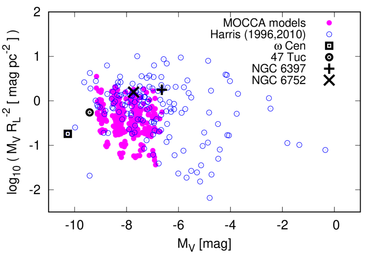
Figure 1: Comparison between observational properties of Galactic GCs (blue open points/histogram) and present-day models (magenta filled points/histogram), where four specific GCs are highlighted (black points). In top panel, we compare the distribution of core to half-light radii. In the middle panel, the x-axis is the cluster V-band absolute magnitude and y-axis is the average surface brightness inside the half-light radius. In the bottom panel, we show the central surface brightness as a function of the core radius. Observational data extracted from Harris (1996, updated 2010).

Among our 288 GC models, there are models which initially collapse due to mass segregation and this initial collapse is halted by binary energy generation or intermediate-mass black hole formation. Subsequently, during the long-term evolution of the GC models, the clusters can again evolve towards core collapse as they exhaust their initial population of binaries that were supporting the cluster evolution via binary burning during the balanced phase. Such GC models can undergo core collpase within a Hubble time and are characterized by smaller initial $T_{\rm rel}$. Such core collapse is deeper and central density becomes large before sufficient number of binaries can dynamically form to prevent further collapse.

With respect to the binary fraction, we notice that for models set with the Kroupa IBP (initially 95 per cent) it drops drastically during the early evolution. This is because most binaries in such models are soft and the denser the cluster, the quicker their disruption. In addition, while comparing predicted and observed binary fractions in GCs, Leigh et al. (2015) were able to conclude that only high initial binary fractions (set with the Kroupa IBP, i.e. binaries with a significant fraction of very wide binaries) combined with high initial densities can reproduce the observed anti-correlation between the binary fraction (both inside and outside the half-mass radius) and the total cluster mass (Milone et al., 2012). Moreover, Belloni et al. (2017c) further investigated the impact of the Kroupa IBP in GCs. These authors compared predicted and observed properties of GC CMDs and managed to further improve properties of initial binaries in order to be incorporated into numerical simulation investigations. They conclude that their modifications to the Kroupa IBP bring present-day GC models even closer to real GCs.

Finally, in order to check whether our models have present-day properties consistent with the Galactic GC population, we show in Fig. 1 a comparison between our models and real GCs. In the top panel, the distributions of core to half-light radii $(R_{c}/R_{L})$ of models and real GCs are shown. In the middle panel, we compare in the plane of absolute magnitude ($M_{V}$) versus average surface brightness ($M_{V}R_{L}^{-2}$). Finally, the central surface brightness ($\Sigma_{c}$) as a function of the core radius ($R_{c}$) is provided in the bottom panel.

Notice that our models lie in the region of massive and intermediate-mass real GCs, and we only miss the low-mass GCs. We also notice that there is a portion of our models in which values of the central surface brightness exceed those of real GCs $(\Sigma_{c}\gtrsim 10^{6}~{}{\rm L}_{\odot}~{}{\rm pc}^{-2})$. Such models have massive intermediate-mass black holes that can have a deeper potential well and this contributes to the increase in central surface brightness. They also contribute to the excess seen in the distribution of core to half-light radii for values in which $\log_{10}(R_{c}/R_{L})<-0.8$. Below this value, $\sim 90$ per cent of the models host an intermediate-mass black hole. More details about influence of black holes in shaping global GC properties can be found in Askar et al. (2018) and Arca Sedda et al. (2018).

Such a comparison clearly shows that we have amongst our models cluster in a reasonable range of concentrations, central surface brightness and relaxation times. To sum up, we showed that our models are consistent with a reasonable part of real GCs. We notice that such a conclusion is not surprising, given that our initial models are similar to part of those shown in Askar et al. (2017), Askar et al. (2018) and Arca Sedda et al. (2018), and these authors managed to show that their models are more or less representative of the Galactic GC population.

In order to properly compare our results with observations, we now separate our models into two groups, which will correspond to our core-collapsed and non-core-collapsed models. Since most core-collapsed real GCs have high central surface brightness ($\Sigma_{c}\gtrsim 10^{3}$ ${\rm L}_{\odot}$ pc^-2) and are very compact ($R_{c}\lesssim 0.2~{}{\rm pc}$), we utilize such values to define our core-collapsed and non-core-collapsed models. The motivation for such a distinction is based on the fact that the observational definition of core-collapsed and non-core-collapsed clusters can be ambiguous. That definition takes into account only the current observational status of the cluster, and not its whole evolution. For instance, Heggie & Giersz (2008) show that M4 (which profile is a classic King profile typical of a non-core-collapsed cluster) is actually a post-collapse cluster, having its core sustained by binary burning. This means that considering the whole cluster evolution, M4 would be a core-collapsed cluster. But when only its current surface-brightness profile is considered, it is classified as non-core-collapsed. In a similar way, Giersz & Heggie (2009) show that NGC 6397 is also a post-collapse GC. This suggests that clusters currently classified as non-core-collapsed could have naturally undergone core-collapse at earlier times and vice versa. Such behaviour is related to the cluster gravothermal oscillations on time-scales of a few hundred million years.

After applying such criteria, we found that the fraction of models considered core-collapsed is only $\sim 30$ and $\sim 20$ per cent, for those set with the Kroupa and the Standard IBPs, respectively. This indicates that our sample of models are mainly composed of models that have properties much closer to non-core-collapsed real GCs than core-collapsed ones.

5 Destruction Rate of Primordial CV Progenitors

We start our analysis quantifying the rate of destruction of primordial CV progenitors with respect to the initial stellar encounter rate, given by $\Gamma=\rho_{0}^{2}r_{c}^{3}\sigma_{0}^{-1}$ (Pooley & Hut, 2006), where $\rho_{0}$, $r_{c}$ and $\sigma_{0}$ are the central density, the core radius and the mass-weighted central velocity dispersion, respectively. We note that $\Gamma$ can be interpreted as an indicator of the strength of dynamics that one would expect during the cluster evolution.

Before proceeding further, it is important to clearly define some terms that will be used in what follows. We call CV progenitors all binaries that somehow become CV and survive up to the present day. Within the CV progenitors, those that are primordial binaries are called primordial CV progenitors. From these definitions, a primordial binary that becomes a CV via CEP, without having its components altered via dynamics, is a primordial CV progenitor. Alternatively, a primordial binary that has, for instance, one of its components replaced in a dynamical exchange interaction is just a CV progenitor. Finally, dynamically or thermally unstable CVs that do not survive up to the present day are not considered in this work.

Figure 2: Fraction of destroyed primordial CV progenitors ($f_{\rm dest}$) versus the initial stellar encounter rate ($\Gamma$). Note the clear correlation between $f_{\rm dest}$ and $\Gamma$.

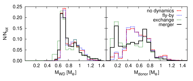
Figure 3: WD mass (left-hand panel) and donor mass (right-hand panel) distributions associated with CVs at their formation times (onset of mass transfer), separated according to each formation channel and normalized by the total number of counts in each formation channel.

We first quantify the fraction of primordial CV progenitors that are destroyed in dynamical interactions before becoming CVs ($f_{\rm dest}$). This is illustrated in Fig. 2, where we show $f_{\rm dest}$ vs. $\Gamma$ for all models, separated according to the IBP and the CEP efficiency. Note that the greater the $\Gamma$, the higher the fraction of destroyed primordial CV progenitors (i.e the stronger the influence of dynamical interactions on destroying these progenitors). In terms of the soft-hard boundary, the greater the $\Gamma$, the shorter the period that defines the boundary between soft and hard binaries.

One interesting fact is that this correlation is stronger for models with the Kroupa IBP. Indeed, we carried out Pearson’s rank correlation tests, and we found strong correlation with more than 99.9 per cent confidence, being $r=0.78$ and $0.70$, for the Kroupa and Standard IBPs, respectively.

It is not difficult to understand why this correlation is stronger for models with the Kroupa IBP, and the reason is intrinsically connected with the period distribution in both IBPs. The majority of the binaries in the Kroupa IBP have periods longer than $10^{3}$ days ($\approx$ 83 per cent), which is not the case for the Standard IBP ($\approx$ 46 per cent). In this way, primordial binaries in the Kroupa IBP are more sensitive with respect to the strength of dynamics, being much easier affected by interactions as a whole, since it is predominantly composed of soft binaries, which is the opposite in the case of the Standard IBP.

After this general overview about CV formation and destruction, we can turn to the analysis of CV population properties, separated according to different formation channels in our models. In all our models, we identify four main formation channels, namely: (i) CEP without any influence of dynamics (no dynamics); (ii) CEP with weak influence of dynamics (fly-by); (iii) exchange; and (iv) merger. More details about how we separate the CVs into these four formation channel groups are given in Belloni et al. (2016, 2017a, 2017b).

6 CV properties

6.1 Progenitor population

We start the presentation of CV properties by focusing our attention on the main distributions (i.e. masses, period, eccentricity and mass ratio) of CV progenitors.

We note that strong dynamical interactions are able to trigger CV formation in binaries that otherwise would never undergo a CV phase, in very good agreement with our previous findings (Belloni et al., 2017a, b). In addition, if we define roughly the range in the parameter space in which primordial CV progenitors belong as $M_{1}/{\rm M}_{\odot}\in[2,5]$, $q\in(0,0.5]$ and $\log_{10}(P/{\rm d})\in[2,5]$, we can compute the fraction of dynamically formed CVs coming from this region. We find that only $\sim$ 23 per cent of all dynamically formed CV progenitors belong to this narrow range, which allows us to conclude that, as previously, dynamics extend the parameter space applicable to CV progenitors (with respect to CVs formed without influence of dynamics), and allow binaries that would not become CVs to evolve into CVs.

6.2 CVs at the onset of mass transfer

If dynamically formed CVs have different properties from CVs formed from primordial binaries, then some of their properties (e.g. component masses and periods) at the onset of mass transfer should be different. Here we discuss two important distributions, the WD mass and the donor mass. The WD mass distribution is important because it can help us to understand the nature of GC CVs, and also because it has been claimed for a long time that GC CVs have, on average, more massive WDs when compared with Milky Way (MW) CVs. The donor mass distribution is important because it determines the entire CV evolution, including the mass transfer rate, and in turn the luminosity, and the duty cycle. In this way, CVs with higher donor masses are more likely to be detected in observational surveys, because they are bright enough or because they exhibit dwarf nova (DN) outbursts more frequently.

In Fig. 3, the WD and donor masses of the CVs at the onset of mass transfer are displayed, separated according to the formation channel. Note that there is no statistical evidence suggesting that the WD mass distribution of dynamically formed CVs is different from that of CVs formed from primordial binaries, since the histograms practically overlap each other. We stress that this result is in disagreement with our previous works (Belloni et al., 2016, 2017a, 2017b), where we do show that these two sets of CVs are different.

The reason for this discrepancy is associated with better prescriptions for CV evolution adopted here, in particular angular momentum loss prescriptions and criteria for dynamically and thermally stable mass transfer, which makes CVs formed from CEP in our simulations to have naturally more massive WDs.

Indeed, we have adopted in all simulations, the eCAML model proposed by Schreiber et al. (2016). According to these authors, if the strength of CAML is inversely proportional to the WD mass, then most (if not all) CVs with low-mass WDs are dynamically unstable. The eCAML model is currently the only model that can solve some long-standing problems, like the associated CV space density, the period distribution and the WD mass distribution (Schreiber et al., 2016; Belloni et al., 2018b). In addition, it can also explain the existence of single He-core WDs (Zorotovic & Schreiber, 2017). The main mechanism thought to be responsible for the postulated dependence of CAML on WD mass are nova eruptions (Schreiber et al., 2016; Nelemans et al., 2016). Such eruptions might cause strong AML by friction that makes most CVs with low-mass WDs dynamically unstable, which leads to merger instead of stable mass transfer. This is because frictional AML produced by novae depends strongly on the expansion velocity of the ejecta (Schenker et al., 1998), and for low-mass WDs, the expansion velocity is small (Yaron et al., 2005).

With respect to the donor mass distribution, we do notice differences between dynamical and non-dynamical CVs. There are relatively more dynamical CVs (formed because of mergers or exchanges) with donors lighter than $\sim 0.3$ M_⊙ (formed during interactions with low-mass binaries). This indicates that dynamics are likely to produce relatively more optically faint CVs than CEP, at the onset of mass transfer.

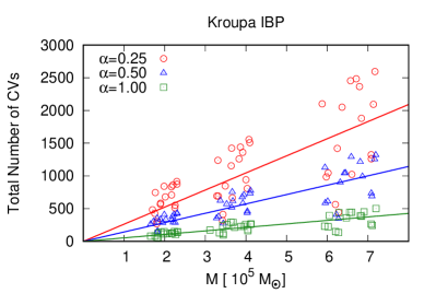
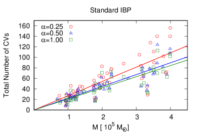
Figure 4: Total number of present-day CVs in all our models against the cluster mass, separated according to the IBP and CEP efficiency. The lines are linear regression models ($N_{\rm tot}=a\times M$, where $N_{\rm tot}$ and $M$ are the total number of present-day CVs and the present-day cluster mass in $10^{5}$ M_⊙, respectively). Note that the value of the CEP efficiency significantly changes the number of CVs in models following the Kroupa IBP. Values of $a$ are provided in Table 2.

6.3 Present-day CV population

One interesting correlation one would expect is related to the number of CVs and GC masses, i.e. the greater the GC mass, the greater the number of CVs. We found here that this correlation holds for all combinations of IBP and CEP efficiency, as illustrated in Fig. 4.

The total amount of present-day CVs in all 288 models is 96214, being $\approx 92.5$ per cent coming from models set with the Kroupa IBP and only $\approx 7.5$ per cent from those set with the Standard IBP. Regarding the CEP efficiency, as expected, the smaller the $\alpha$, the greater the number of CVs, i.e. models set with $\alpha=0.25$, $0.5$ and $1.0$ contribute with $\approx 56.5$, $\approx 30.5$ and $\approx 13.0$ per cent, respectively.

Table 2: Coefficient for the best-fitting lines in the plane total number of CVs versus present-day cluster mass, in the form of $N_{\rm tot}~{}=~{}a~{}\left(M/10^{5}{\rm M}_{\odot}\right)$, for all models in our simulations grouped according to the IBP (Kroupa or Standard) and the CEP efficiency ($\alpha=$0.25, 0.50 and 1.00). The lines are plotted in Fig. 4.

Kroupa IBP $\alpha$ 0.25 0.50 1.00 $a$ $266.1\pm 14.9$ $143.0\pm 6.3$ $53.4\pm 2.3$ Standard IBP $\alpha$ 0.25 0.50 1.00 $a$ $27.1\pm 1.3$ $22.4\pm 0.9$ $21.1\pm 0.9$

In order to provide readers a way to estimate the amount of CVs per GC mass, we performed linear regressions for the number of CVs against the host GC mass, in the form $N_{\rm tot}~{}=~{}a~{}\left(M/10^{5}{\rm M}_{\odot}\right)$, for all models in our simulations grouped according to the IBP and the CEP efficiency. The best-fitting coefficients are provided in Table 2 and the best-fitting lines are plotted in Fig. 4.

From Fig. 4, we clearly see that the number of CVs significantly changes with regards to $\alpha$, for models set with the Kroupa IBP. On the other hand, for models set with the Standard IBP, the number of CVs is almost insensitive with respect to $\alpha$. This result is a direct consequence of the respective period distributions. As the period distribution in the Kroupa IBP smoothly increases towards longer periods, the smaller the alpha, the higher the amount of CVs that survive the CEP, since lower values for $\alpha$ lead to shorter periods after CEP. In this way, since the number of binaries increases with period in the Kroupa IBP, more and more binaries manage to become CVs due to the fact that the pre-CV lifetimes are reduced, as the value of $\alpha$ becomes smaller. Now, for the Standard IBP, since the period distribution is log-uniform throughout the entire range of period, the effect of moving the range from which CV progenitors belong towards longer periods (by decreasing $\alpha$) has only a small effect on the amount of CVs formed.

In what follows, we concentrate only on observational properties related to GC CVs. In other words, hereafter we only investigate properties of present-day CVs that are likely to be observed via multiple technique methods, since these are the most important ones and can potentially lead to some constraints.

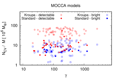
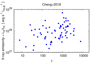
Figure 5: In the left-hand panel, we show results of our models for the number of both, detectable and bright CVs per unit mass vs. the mass-normalized stellar encounter rate ($\gamma$). We separated the models with respect to the IBP (i.e. Kroupa and Standard). In the right-hand panel, we show observational results by Cheng et al. (2018). The X-ray emissivity, defined as the ratio between the X-ray luminosity and the K-band luminosity $(L_{X}/L_{K})$, is considered a measure of the number of X-ray source abundance in a GC (in the study of these authors, mainly CVs and ABs). Note that, in both panels, there is no (if at all very weak) statistical evidence for a correlation between the CV abundance or faint ($L_{X}\lesssim 10^{34}$ erg s^-1) X-ray sources and $\gamma$.

7 Present-day CV Population: detectable CVs

7.1 Criteria to be considered detectable

So far we know that core-collapsed GCs show 2 populations of CVs (Cohn et al., 2010; Lugger et al., 2017), and that based on that we can separate the CV population for non-core-collapsed GCs (Cool et al., 2013; Rivera Sandoval et al., 2018). In order to investigate whether we can reproduce some observational features of these two populations, we first select the detectable CVs in our models. To do so, we assume a conservative definition in order to allow for statistical analysis and to be consistent with observations. We used as cut-offs the donor mass, X-ray luminosity and the absolute visual magnitude, being the last two computed as described in Belloni et al. (2016) and assuming that the average accretion rate onto the WD during quiescence is 1 per cent of the average mass transfer rate. Our limiting quantities are: donor mass is $0.1$ M_⊙, X-ray luminosity is $5\times 10^{29}$ erg s^-1 and the limiting absolute visual magnitude is 14 mag (i.e. 10 mag below the turn-off magnitude). These three values are consistent with observational limits (Cohn et al., 2010; Cool et al., 2013; Lugger et al., 2017; Rivera Sandoval et al., 2018; Henleywillis et al., 2018).

From the total of 96214 present-day CVs in all our simulations, after applying these criteria, we have 2129 detectable CVs. This provides that, on average, only between $2-4$ per cent (depending on the CEP efficiency) of the CVs in a GC can eventually be detected.

We now separate the detectable CVs between bright and faint. Bright CVs presumably have their optical fluxes dominated by the donor. Whereas faint CVs have theirs dominated by the WD and/or accretion disc. To be consistent with observations, we adopt here a cut-off based on the absolute visual magnitude, which is defined by $M_{V}$=9 mag. Detectable CVs which absolute visual magnitudes are smaller than that are bright CVs, and they are faint otherwise. We emphasize that this criterion is suitable for our purposes, since our goal is to infer statistical properties from our models rather than modelling particular GCs.

After filtering out the CVs with respect to limiting luminosities and separating them according to their brightness, an additional and final criterion has to be applied, regarding the position in the cluster. In observations, the observed region is usually within the half-light radius ($R_{L}$), and for this reason, in some comparisons with observations, we also separate them with respect to $R_{L}$.

7.2 Influence of the cluster type

With respect to the cluster type, for those models set with the Kroupa IBP, we notice that most core-collapsed models have fractions of bright CVs with respect to detectable CVs in the range of $5-45$ per cent, and most non-core-collapsed models have them in the range of $7-33$ per cent. However, a small portion of our core-collapsed models have more than $50$ per cent of bright CVs. These models are compact and characterized by high values of the central surface brightness, and short half-mass relaxation times. These models have then properties much closer to real core-collapsed GCs than the whole set of our core-collapsed clusters.

On the other hand, for models set with the Standard IBP, most of them have none bright CVs ($\sim 90$ per cent of them), and only a few have non-null fractions of bright CVs. We can conclude then that, in general, such an IBP cannot reproduce observed fractions of bright CVs among core-collapsed and non-core-collapsed clusters.

The fractions of bright CVs we found for models set with the Kroupa IBP are, in general, consistent with observations of non-core-collapsed GCs ($\sim 20-25$ per cent). They are also consistent with respect to core-collapsed GCs ($\sim 40-60$ per cent), provided we take into account only models whose properties are much closer to observed core-collapsed GCs.

Regarding the detectable CV spatial locations, we found that, on average, only $\sim 45$ per cent of detectable CVs (both bright and faint) are inside the half-light radius, which corresponds to $\sim 42$ and $\sim 47$ per cent of bright and faint CVs, respectively, inside it. However, such fractions should be considered upper limits as they depend on the cluster properties. In particular, as shown in Section 7.5, such fractions of detectable CVs inside/outside $R_{L}$ strongly depends on the cluster half-mass relaxation times.

7.3 Are most CVs dynamically formed?

With respect to the formation channels, the dominant one amongst detectable CVs is typical CEP ($\approx 88^{+12}_{-18}$ per cent, for both core-collapsed and non-core-collapsed clusters). We also found that the average fraction of dynamically formed CVs among only bright CVs is relatively low ($\approx 9_{-9}^{+24}$ per cent, for both core-collapsed and non-core-collapsed clusters). In other words, we found here no (if at all very weak) correlation between the number of either detectable CVs or bright CVs with respect to the cluster type (e.g. related to the stellar encounter rate).

Our results are in disagreement with previous conclusions that bright CVs were predominantly dynamically formed (via exchange), and faint CVs were a mix of CVs formed in different channels (Belloni et al., 2017b; Hong et al., 2017). This is likely connected with the high (non-realistic) CEP efficiency adopted previously, since the higher the CEP efficiency, the smaller the number of CVs formed from primordial binaries, especially for models following the Kroupa IBP. In this way, the contribution from primordial CVs have been underestimated in our previous works.

We note that our current findings are in agreement with recent studies of Chandra X-ray sources in GCs by Cheng et al. (2018). Using a sample of 69 GCs and focussing on CVs and chromospherically active binaries (ABs), these authors found that there is not a significant correlation between the number of X-ray sources and the mass-normalized stellar encounter rate in units of $10^{6}~{}{\rm M}_{\odot}$ ($\gamma=\Gamma/M_{6}$). These findings disagree with previous results, which considered smaller GC samples (e.g. Pooley & Hut, 2006). A correlation would be expected if dynamical interactions largely influence the creation of X-ray sources. However, Cheng et al. (2018) have shown that dynamical interactions are less dominant than previously believed, and that the primordial formation has a substantial contribution. In Fig. 5 we show the number of CVs as a function of $\gamma$. We show numbers for both, detectable and bright CVs normalized by the total cluster mass in units of $10^{6}~{}{\rm M}_{\odot}$. In that figure we also show results from Cheng et al. (2018) for the X-ray emissivity (defined by these authors as the X-ray luminosity divided by the K-band luminosity and considered a measure of the X-ray source abundance, mainly CVs and ABs) vs. $\gamma$. Note that both observational and theoretical results show no (if at all very weak) statistical evidence for a correlation between the normalized CV abundance and $\gamma$.

The physical reason for that is associated with the role of dynamics in creating and destroying pre-CVs. We notice that destruction of CV progenitors take part mainly for MS-MS binaries during the first few hundred Myr of cluster evolution. Later, when MS-WD binary is created, dynamical interactions are very strongly suppressed, because during the CEP there is a substantial reduction of binary periods.

Regarding dynamical pre-CV formation, one can have mainly three possible scenarios:

i) interaction between a low mass MS-MS binary and single C/O WD: this type of interaction would lead to exchange interaction in which a MS is replaced with a WD. Such an interaction has to form rather compact binary, since the binary evolution needs about $\lesssim 10$ Gyr to make it a CV. If the exchanged binary is wider (say two times), then it will need several dynamical interactions to bring it to the period which will result in CV formation. Since the Spitzer’s average change of binding binary energy is 20 per cent (Spitzer, 1987), it would be needed around four such interactions, which is rather not probable for large number of such binaries.

ii) interaction between a low mass MS-MS binary and single MS: this interaction would lead to an MS-MS binary which, before WD formation, is brought to the adequate range (Section 6.1) that will guarantee CEP and further binary evolution (during $\sim 10$ Gyr) leading to CV formation. We found that the average number of such interactions is only $\sim 0.05$ per CV, which clearly shows that this channel is not important.

iii) interaction between a WD-MS binary and single MS: there are two posibilities here, either this interaction is strong and generates a pre-CV via the replacement of the MS in the binary with a more massive MS intruder, or a few interactions occur which harden such a WD-MS binary to become a pre-CV. For this scenario, the probability is also low, provided the small average semi-major axis of WD-MS binaries ($\sim 10{\rm R}_{\odot}$) and typical properties of GCs inferred from the models. Indeed, the average numbers of weak and strong interactions associated with pre-CV binaries over the time-scale of $\sim 10$ Gyr (time between WD-MS binary and CV formations) are $\sim 0.126$ and $\sim 0.003$ per CV, respectively.

To sum up, we show that the main scenarios proposed in the literature (Ivanova et al., 2006; Shara & Hurley, 2006; Belloni et al., 2016, 2017a, 2017b; Hong et al., 2017) for dynamical formation of faint and bright CVs in GCs have very low probability to happen, which explains our findings with respect to the influence of dynamics in CV formation (very low fraction of dynamically formed faint and bright CVs) and with respect to the stellar encounter rate (no/extremely weak correlation with the amount of detectable and bright CVs). We notice that our explanation is supported by recent observations (Cheng et al., 2018), which show that there is no (or very weak) correlation between faint ($L_{X}\lesssim 10^{34}$ erg s^-1) X-ray sources, presumably mainly composed of CVs and ABs, and $\gamma$.

Figure 6: X-ray luminosity, absolute visual magnitude, donor mass and period distributions associated with detectable CVs (i.e. bright and faint CVs). Each histogram was normalized by the total amount of detectable CVs. Vertical lines in the period distribution are the observational location of the period minimum (Gänsicke et al., 2009) and gap edges (Knigge, 2006). Notice that bright CVs are mainly above the gap (with some inside it) and most faint CVs are below the gap (with a few right above it).

Figure 7: Some CV properties against period: X-ray luminosity (top left-hand panel), absolute visual magnitude (top right-hand panel), donor mass (bottom left-hand panel) and mass transfer rate (bottom right-hand panel). Vertical lines are the observational location of the period minimum (Gänsicke et al., 2009) and gap edges (Knigge, 2006).

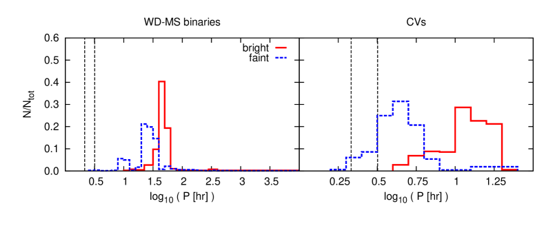
Figure 8: Normalized formation rates (top row) of WD-MS binaries that will later become the detectable CVs (left-hand panel) and of detectable CVs (right-hand panel), and their period distributions (bottom row). Vertical lines in the period distributions are the observational location of the gap edges (Knigge, 2006). Note that most WD-MS binaries (pre-CVs) are formed before $\sim~{}1$ Gyr and most CVs are formed after $\sim~{}10$ Gyr.

7.4 Orbital, photometric and X-ray properties

In order to check whether we are able to reproduce the bimodality of GC CVs, we show in Fig. 6 the distributions of the absolute visual magnitude, X-ray luminosity, donor mass and period for all detectable CVs. Note that we have indeed evidences towards a bimodal population, even though the population of faint CVs is clearly dominant in the four distributions. In particular, it is interesting that we find a bimodality in the X-ray luminosity distribution, where we have a population of faint X-ray CVs ($L_{X}\lesssim 10^{31}$ erg/s) and another population of bright X-ray CVs ($L_{X}\gtrsim 10^{31}$ erg/s), which actually is in good agreement with observations (Rivera Sandoval et al., 2018, see their fig. 14). However, we note that detectable CVs with X-ray luminosities below $10^{30}$ erg/s are missing in our distribution, whereas CV candidates have been observed below that limit. This observed population of very faint X-ray CVs likely have extremely low-mass donors ($<0.1$ M_⊙), and periods close to the period minimum (period bouncers or their progenitors). In fact, some Galactic field CVs, such as GW Lib and WZ Sge, which have X-ray luminosities $0.05^{+0.10}_{-0.02}\times 10^{30}$ and $0.7^{+0.3}_{-0.1}\times 10^{30}$ erg s^-1 [2-10 keV], respectively (Byckling et al., 2010), seem to support this explanation. Alternatively, we notice that such X-ray luminosities could also be reached in cases where the time-averaged accretion rate in short-period CVs would be smaller than the one assumed here (i.e. $<~{}10^{-2}~{}\langle\dot{M}_{\rm tr}\rangle$, where $\langle\dot{M}_{\rm tr}\rangle$ is the time-averaged mass transfer rate).

Regarding the period distribution of the detectable CVs, we see that bright systems dominate the distribution above the period gap. Whereas the faint systems have periods shorter than 4h, with a vast majority below the period gap. Note, however, that the gap is populated by both types of CVs. In Fig. 7. we show how the orbital period of the detectable and non-detectable CVs are related to the X-ray luminosity, absolute visual magnitude, donor mass and mass transfer rate. From this figure we see that bright CVs have longer periods, higher mass transfer rates, higher donor masses and higher luminosities. This is in general agreement with the properties found for the bright CVs in the 4 GCs that we are considering, which have periods longer than 2.4 h (see e.g. Bailyn et al., 1996; Kaluzny & Thompson, 2003; Rivera Sandoval et al., 2018, and references therein). Unfortunately CVs below the period gap have not been confirmed in any of these clusters. From Fig. 7 we can also clearly see the typical trend associated with CV evolution, which goes from long to short periods. Note that due to our chosen mass limit for detectable CVs (M${}_{\rm donor}>0.1$ M_⊙), we miss in these plots the portion of extremely faint CVs composed of period bouncers. Our results then suggest that those CV candidates in NGC 6397, NGC 6752, 47 Tuc and $\omega$ Cen with very low luminosities, are likely period bouncers or CVs very close to the period minimum (WZ Sge-type).

Figure 9: Cumulative radial distribution function (CDF) for detectable CVs (faint and bright), for clusters grouped according to different half-mass relaxation times ($T_{\rm rel}$): $T_{\rm rel}/$Gyr < 4 (top left-hand panel), 4< $T_{\rm rel}/$Gyr < 8 (top right-hand panel), 8< $T_{\rm rel}/$Gyr < 15 (bottom left-hand panel), $T_{\rm rel}/$Gyr > 15 (bottom right-hand panel). We also indicate in each panel the mean values of $T_{\rm rel}$, and bright and faint CV masses ($M_{\rm b}$ and $M_{\rm f}$, respectively). Note that, mean values of $M_{\rm b}$ and $M_{\rm f}$ are similar in all panels and that, for different $T_{\rm rel}$, bright and faint CVs show different levels of concentration relative to the MSTO stars.

Figure 10: Cumulative radial distribution function (CDF) for detectable CVs (faint and bright), for clusters which half-mass relaxation times ($T_{\rm rel}$) are shorter than 4 Gyr. We separated the faint CVs into three groups, according to their masses, namely (i) $M<0.8$ M_⊙ (blue curve), (ii) $0.8<M/$M${}_{\odot}<1.2$ (green curve), and (iii) $M>1.2$ M_⊙ (orange curve). In the keys we provide the average mass of each stellar group, i.e. MSTO stars, bright CVs, and faint CVs separated as described above. Note that, different faint CV masses show different levels of concentration relative to the MSTO stars.

7.5 Spatial Distribution: general features

From the discussion so far, it is clear that the dominant formation channel amongst bright and faint CVs is the typical CEP, as in MW CVs. In this way, a natural follow-up concern is how to explain their properties, including their spatial distributions. Interestingly, Cohn et al. (2010) and Lugger et al. (2017) suggest that their findings are consistent with an evolutionary scenario in which CVs are produced by dynamical interactions near the cluster centre and diffuse to larger orbits as they age. However, the results of our simulations suggest that this scenario is not very likely. Indeed, a CV that is dynamically formed in a cluster core is ejected outside the central parts due to the strength of the dynamical interaction. Thus, it is unlikely that it will remain in the core after formation. In addition, the probability for a CV to interact is extremely small, given their short periods (Leigh et al., 2016; Belloni et al., 2017a). In this way, scattering interactions acting to increase their orbits and thus, forcing their migration to larger radii in the cluster potential are not very likely. Finally, such a scenario seems to ignore completely the contribution of primordial CVs to the present-day CV population.

In order to provide readers a scenario which is compatible with our findings, we should consider the WD-MS binary and CV formation times, their properties at the formation times, and the cluster $T_{\rm rel}$.

In Fig. 8, we show the normalized formation rate of CVs and WD-MS binaries that are their progenitors, separating them into bright and faint populations. Note that most WD-MS binaries are formed before $\sim 1$ Gyr, which is the time for the formation of most C/O WDs, given the metallicity adopted here (Z=0.001). The remaining WD-MS binaries that are formed after this time are mainly dynamical ones. On the other hand, the detectable CVs are formed mainly after $\sim 10$ Gyr, which is more or less the limiting time for them to be bright enough to be detected at the present day (i.e. at 12 Gyr). In this way, the time required for a CV to evolve beyond the detection limit is around $\sim 2$ Gyr, which is consistent with the time-scale associated with long-period CVs to evolve towards close to the period minimum (donor mass of $\lesssim 0.1$ M_⊙).

Said that, we reach the following general picture related to the origin of faint and bright CVs. Since most of them are formed via CEP under no/weak influence of dynamics and since CVs have C/O WDs, the WD-MS binaries should have to be formed during the early cluster evolution, but they should have periods such that systemic angular momentum losses should take more than $9$ Gyr to shrink their orbits such that they become interacting binaries, i.e. CVs. This is precisely the case as seen in Fig. 8. Note that most WD-MS binaries that are progenitors of bright CVs are born with periods longer than $\sim 30$ hr. On the other hand, most of those that are faint CV progenitors are born with periods between $\sim 10$ and $\sim 30$ hr. With such long periods, it is not surprising that they take more than 9 Gyr to become CVs.

In this picture, the mass segregation comes naturally, since the WD-MS binaries are very hard to interact strongly during the cluster evolution and have their properties changed (e.g. Leigh et al., 2016; Belloni et al., 2017a), but they could have enough time to sink towards the core, if the $T_{\rm rel}$ is short enough to allow that. This occurs for both bright and faint CVs, as their masses (including both components, the WD and MS star) are, on average, $\sim 1.42\pm 0.19$ and $\sim 1.11\pm 0.21$ M_⊙, respectively, i.e. they are more massive than the cluster average mass within the half-mass radius. We emphasize that this would happen if the cluster half-mass relaxation is substantially shorter than the Hubble time, especially because the WD-MS progenitors are initially amongst the most massive objects in the cluster and segregation starts already at the very beginning.

In general, the shorter the $T_{\rm rel}$, the faster the mass segregation within such a cluster. In addition, as bright and faint CVs are more massive than MSTO stars, the shorter the $T_{\rm rel}$, the more the mass segregation of CVs with respect to these stars. If $T_{\rm rel}$ is short enough, say $\lesssim$ 3 Gyr, then differences between bright and faint CVs also become clear, since bright CVs are, in general, more massive than faint CVs. Indeed, at the present day, faint CVs are less massive either because they already evolved as CVs or because their donor masses are initially small and the onset of mass transfer is close to the present day. Thus, in the case when the cluster half-mass relaxation time is much shorter than the Hubble time, we should expect stronger differences between bright and faint CV spatial distributions, being bright CVs much more segregated than the faint ones.

Figure 11: Illustrative CV radial position evolution, together with the host cluster core and half-mass radii evolution. The cluster evolves towards core collapse until $\approx 0.5$ Gyr when the core bounce occurs, the pre-CV is formed due to dynamical exchange at $\approx 6.7$ Gyr and the CV is formed close to the present day. Note that due to the strong interaction, the newly formed pre-CV is expelled from the central parts, but returns to it due to mass segregation.

In order to better understand how CV spatial distribution depends on the cluster half-mass relaxation time, we first separate all models having initially 1200k objects (due to their higher number of CVs) into four groups according to their relaxation times, namely (i) $T_{\rm rel}/$Gyr < 4, (ii) 4< $T_{\rm rel}/$Gyr < 8, (iii) 8< $T_{\rm rel}/$Gyr < 15, (iv) $T_{\rm rel}/$Gyr > 15. In Fig. 9 we depict the cumulative radial distribution function for detectable CVs (faint and bright), for clusters grouped according to the above-mentioned ranges of $T_{\rm rel}$. Note first that the average mass of bright and faint CVs, in all panels, are quite similar, being $\sim 1.4\pm 0.2$ and $\sim 1.0\pm 0.2$ M_⊙ so that differences in mass segregation should come mainly because of differences in $T_{\rm rel}$. In the bottom right-hand panel, $T_{\rm rel}$ is much longer than the Hubble time, which implies that there is no visible difference between CVs and MSTO stars, since they do not have enough time to separate inside the cluster. In the bottom left-panel, $T_{\rm rel}$ is slightly shorter than the Hubble time and there is a small difference between CVs and MSTO stars. As $T_{\rm rel}$ decreases further, the difference between CVs and MSTO stars becomes more and more clear, as illustrated in top right-hand panel, where $T_{\rm rel}\sim 5-6$ Gyr. By decreasing even further, differences between bright and faint CVs become more and more clear, as seen in top left-hand panel for clusters whose half-mass relaxation times are $\sim 3-4$ Gyr. Thus, to sum up, the shorter the $T_{\rm rel}$, the faster and efficient the mass segregation of bright CVs with respect to faint CVs, and faint CVs with respect to MSTO stars.

Now, in order to better understand how the mass segregation changes with respect to the faint CV masses, we show in Fig. 10 the cumulative radial distribution function of bright and faint CVs for clusters whose $T_{\rm rel}~{}<~{}4$ Gyr, separating the faint CVs into three groups, according to their masses, namely (i) $M_{f}<0.8$ M_⊙ (blue curve), (ii) $0.8<M_{f}/$M${}_{\odot}<1.2$ (green curve), and (iii) $M_{f}>1.2$ M_⊙ (orange curve). Note that the smaller the faint CV masses, the weaker the mass segregation with respect to MSTO stars. If $T_{\rm rel}$ is conveniently short, as faint CVs evolve and become less massive, their level of segregation will quickly adjust to that of MSTO stars. In this way, the ‘speed’ of segregation of faint CVs decreases as they evolve and reduce their masses. In any event, they keep segregating, but not as ‘fast’ as before, because they are less massive now. In the case they have masses similar to MSTO stars, they should segregate in a similar fashion. In the case they are more massive, then they would segregate more than MSTO stars. Thus, not only the cluster $T_{\rm rel}$ is important for mass segregation, but also the CV masses and the rates of mass decrease.

Figure 12: Number of detectable CVs in our models against the cluster mass, separated according the IBP and CEP efficiency. Observational numbers obtained from Bassa et al. (2004, M 4), Cohn et al. (2010, NGC 6397), Lugger et al. (2017, NGC 6752) and Rivera Sandoval et al. (2018, 47 Tuc). For consistency with the other clusters, in the case of 47 Tuc the plotted number corresponds to the CVs detected in the optical filters and not to the whole NUV CV sample reported by these authors. Observational masses were extracted from Kimmig et al. (2015) and Heyl et al. (2012). Vertical error bars correspond to Poisson errors.

Provided these features about CV segregation, the spatial distributions for NGC 6397, NGC 6752, 47 Tuc and $\omega$ Cen can be easily explained. Both core-collapsed clusters (NGC 6397 and NGC 6752) have very short $T_{\rm rel}$ ($\lesssim 0.7$ Gyr), which makes the movement of their bright and faint CV population relatively fast. In addition, as their faint CVs have masses similar to MSTO stars, they are as segregated as MSTO stars. On the other hand, the $T_{\rm rel}$ of 47 Tuc is longer ($\sim 3$ Gyr), but according to Fig. 10, still short enough to allow differences between bright and faint CVs, if their masses are different. However, if the masses of CVs in 47 Tuc are similar in both bright and faint CVs, as suggested by Rivera Sandoval et al. (2018), even if its $T_{\rm rel}$ is short, the faint CV population would still be as segregated as bright CVs and more centrally concentrated than MSTO stars, as shown in Fig. 10. On the other hand, Henleywillis et al. (2018) found that most of the CVs in $\omega$ Cen reside outside the central region, with only the two most luminous CVs lying deep inside the core. These results suggest that indeed the CVs in that cluster have not segregated towards the core given its large $T_{\rm rel}$.

In general, we expect that in GCs, both bright and faint CVs at the onset of mass transfer are more centrally concentrated than MSTO stars, due to their history during the course of the cluster evolution, not because they are mostly dynamically formed in the core.

7.6 Spatial Distribution: dynamically formed CVs

We notice that we can also explain the spatial distribution of the bright CVs that are dynamically formed close to the present-day, in core-collapsed GCs. If a pre-CV is dynamically formed in the core, it cannot stay in the core after the formation, as the process of forming a pre-CV dynamically is very energetic and such a pre-CV will be expelled far from the core. However, if the cluster half-mass relaxation time $T_{\rm rel}$ is short enough (as in core-collapsed GCs) to allow the pre-CV to segregate before it becomes a CV, such a population can come back to the central parts. Thus, forming a bright CV in the central parts. If $T_{\rm rel}$ is relatively long, those bright CVs that are dynamically formed will be found far from the central parts.

This process is illustrated in Fig. 11, where we show the radial position evolution for one dynamically formed CV (together with the host cluster radii evolution). Such a model is evolving towards collapse until about $0.5$ Gyr, when the 10 per cent black hole Lagrangian radius reaches its minimum. This is when the core bounce (Breen & Heggie, 2013) occurs and the black holes generate sufficient energy to support the whole cluster evolution. As such a cluster is supported by a subsystem of black holes, the energy generation is relatively large, which causes the cluster to expand (Breen & Heggie, 2013), and the whole black hole subsystem stops to mass segregate at about 1.2 Gyr. Such a feature leads to an increase in $T_{\rm rel}$ during the cluster evolution, and close to the present day, $T_{\rm rel}\approx 3.5$ Gyr.

Regarding the CV, we notice that its progenitor (MS-MS binary) also initially segregates, as it is one of the most massive objects in the cluster. At the moment the core bounce occurs, the CV progenitor is violently ejected from the core in a four-body interaction with another MS-MS binary. After that it takes around $5$ Gyr to segregate back to the core. However, during this time, the binary starts unstable mass transfer and merges (due to the high initial mass ratio) at $\approx 1$ Gyr, leading to the formation of a single WD. After the single WD returns to the core, it interacts with MS-MS binary and one of such MS stars is replaced with the single WD, leading to a WD-MS binary at $\approx 5.5$ Gyr. Such a binary is dissolved in a three-body interaction with a single MS star at $\approx 6.5$ Gyr. After that, the single WD interacts again with a MS-MS binary at $\approx 6.7$ Gyr, which leads to the pre-CV formation when again a MS star is replaced with the WD intruder. Notice that right after the pre-CV formation in the core, the pre-CV is kicked out from there, and takes a few Gyr ($\approx 3$ Gyr) to segregate back to the inner parts. That time is consistent with $T_{\rm rel}$. In this way, dynamically formed CVs in cluster with shorter $T_{\rm rel}$ are expected to migrate back inwards faster. In other words, the shorter $T_{\rm rel}$, the faster the dynamically formed CV segregates back to the inner parts, after being ejected from the core due to the strong interaction. This particular CV formation (i.e. onset of mass transfer) takes place close to the present day.

7.7 Predicted number of detectable CVs and observed number of CVs and CV candidates

After all this discussion about CV properties, we can now attempt to provide some useful constraints for GC modelling. To do so, we show in Fig. 12 the number of detectable CVs within $R_{L}$ against the cluster mass, including the observational results. We separate the models according to the IBP (Standard and Kroupa) and the CEP efficiency ($\alpha=$ 0.25, 0.50 and 1.00).

From Fig. 12, it is clear that the number of detectable CVs strongly depends on model assumptions, and clusters with similar present-day masses can have very different numbers of detectable CVs. In any event, the maximum number of detectable CVs (for models clustering around a particular mass) is still higher for greater GC masses, which is consistent with results for the entire CV population (see Fig. 4). The fact that the number of detectable CVs depends on model assumptions is quite convenient for us, since we can confront them against observations and infer what are the assumptions that are likely to lead to consistent results.

With respect to the IBP, we can see that our 144 models set with the Standard IBP are unlikely to reproduce observations, with the exception of M4. They have always $\lesssim 5$ detectable CVs per cluster, irrespective of initial conditions and stellar/binary evolution parameters, and they have present-day masses roughly consistent with NGC 6397, NGC 6752 and M4. On the other hand, models set with the Kroupa IBP are more likely to reproduce observational results for the four clusters considered here. Indeed, when taking into account error bars and models with largest numbers of detectable CVs, and/or shortest $T_{\rm rel}$, the observed amount of CVs in 47 Tuc, NGC 6397, NGC 6752 and M4 are in a rough agreement with our results. So, as we are not modelling particular GCs, we can conclude that our results are roughly in agreement with observations, specially provided the small number statistics related to GCs with deep observations regarding CVs.

Regarding the CEP efficiency, we notice that models evolved with $\alpha=0.25$ and $0.5$ better reproduce the observed amounts of CVs. This is not the case when $\alpha=1$ is considered, which leads to smaller numbers of detectable CVs. This result is consistent with the fact that the smaller the $\alpha$, the greater the amount of CVs.

It is interesting though that, our results suggest that the long-standing problem related to the deficit of CVs in GCs can potentially be solved, while carefully including in the modelling appropriate IBP, CV formation/evolution prescriptions and observational selection effects. We also note that a conclusive answer for that is out of the scope of this work, as we would need many more models such that the GC initial parameter space would be better filled (see Table 1).

Notice that $\omega$ Cen was not included in this analysis. This is because its mass is much larger than the other GC masses and we do not have amongst our models any that massive. However, we can extrapolate results presented in Section 6.3 in order to account for $\omega$ Cen. Assuming that best results are for the Kroupa IBP, low CEP efficiency and considering that $\approx 2-4$ per cent of all CVs should be detectable (and only $\approx 50$ per cent of them are inside $R_{L}$), we predict that there should be $\approx 50-250$ detectable CVs inside the half-light radius of $\omega$ Cen. This number is at least $\approx 2$ times higher than the observed amount of CVs in that cluster. In addition, a better optical characterization and membership determination of the unclassified X-ray sources in that cluster may increase the number of detected CVs. For example, Henleywillis et al. (2018) extrapolated their results and estimated that there must be $\sim 40\pm 10$ CVs with $L_{X}\geq 10^{30}$ erg s^-1, but several less luminous CVs must be present.

8 Discussion

We have analysed a relatively large sample of 288 GC models, evolved with an up-to-date version of the mocca code, with respect to IBPs and stellar/binary evolution prescriptions. These models have a variety of different initial conditions spanning different values of the mass, size, King parameter, IBP, binary fraction, and Galactocentric distances. In addition, we also explored two parameters of stellar/binary evolution, namely inclusion or not of fallback and three different CEP efficiencies.

With respect to dynamical production and destruction of CV progenitors, our results suggest that we should expect less CVs in dense GCs relative to the MW field, due to the fact that destruction of CV progenitors is more important in GCs than dynamical formation of CVs. Indeed, all our models have mass densities smaller than $\sim 8.5\times 10^{-5}$ CVs M$\odot^{-1}$, which is smaller than the one in the Galactic field ($\sim 10^{-4}$ CVs per M_⊙). This is in agreement with results found by Cool et al. (2013) for the massive cluster $\omega$ Cen. These authors determined a mass density of $\sim 1.4\times 10^{-5}$ CVs per M_⊙, which is consistent with our derived average density ($\sim 2\times 10^{-5}$ CVs M$\odot^{-1}$), and about 1 order of magnitude smaller than the one in the Galactic field. We notice that this is also consistent with 47 Tuc, which has a CV mass density of $\sim 7\times 10^{-5}$ CVs M${}_{\odot}^{-1}$, i.e. smaller than in the MW. Finally, our results are also in agreement with recent analysis of archival Chandra data by Cheng et al. (2018). These authors analysed 69 GCs and conclude that, different from what has been previously thought, the weak X-ray populations, primarily CVs and ABs, are under-abundant in GCs with respect to the Solar neighborhood and Local Group dwarf elliptical galaxies.

In addition, our results are also in agreement with the concentration of CVs found in $\omega$ Cen. Cool et al. (2013) and Henleywillis et al. (2018) found that there is no much difference in the radial distribution between bright and faint CVs, which is in line with our Fig. 9, since $\omega$ Cen has a very long $T_{\rm rel}$. We stress that the radial distribution of CVs in GCs is not indicative of their formation channel, as suggested previously (e.g. Davies, 1997), but rather a consequence of the GC properties, mainly $T_{\rm rel}$, and the CV masses.

We found that, on average, more than half of the entire population of detectable CVs are outside the half-light radius, and future observations could aim to search for X-ray sources in regions not close to the cluster centres. However, we notice that this should be considered an upper limit, as the real fraction of CVs outside the half-light radius varies from cluster to cluster and depends mainly on its $T_{\rm rel}$. Indeed, in Fig. 9 and 10 we show that (i) the greater the CV mass, the stronger the effect of mass segregation and, (ii) the shorter the cluster’s $T_{\rm rel}$, the stronger the effect of mass segregation. Said that, we expect that clusters with relatively long $T_{\rm rel}$ (longer than a few Gyr) will have a considerable amount of CVs outside their half-light radius and the opposite for cluster with short $T_{\rm rel}$ (shorter than a few hundreds of Myr). Our results then suggest that in clusters where $T_{\rm rel}$ are relatively long, we would be able to roughly double the number of GC CV candidates while looking for them outside $R_{L}$. This would also allow us to obtain accurate spectra since the crowding should not be a big problem in the regions far away from the GC centres.

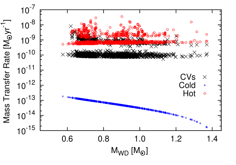
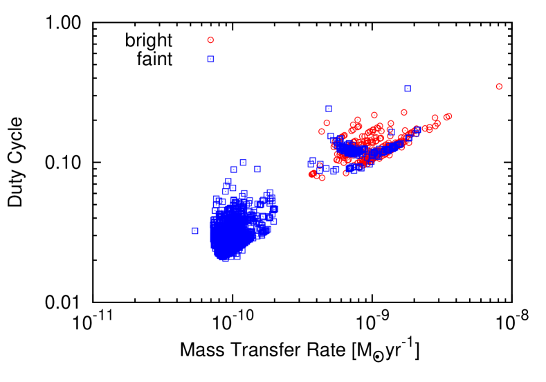
Figure 13: Top panel: comparison of the values of the mass transfer rate required for a full CV disc to be globally hot and stable or globally cold and stable (computed as described in Belloni et al., 2016) with respect to the mass transfer rate of detectable CVs. Bottom panel: Duty cycle (computed with the empirical relation provided in Britt et al., 2015) versus the mass transfer rate for the detectable CVs in the simulation.

One important long-standing question related to GC CVs is whether they are predominately magnetic or not. In order to test the hypothesis that most CVs in GCs are actually dwarf novae (DNe) with very short duty cycles, we first separate all detectable CVs according to the stability in the accretion disc and compute their duty cycles. In the top panel of Fig. 13 we show the values of the mass transfer rate required for a full CV disc to be globally hot and stable or globally cold and stable (computed as described in Belloni et al., 2016) with respect to the mass transfer rate of detectable CVs. It clearly shows that more than 99 per cent of all detectable CVs in our 288 models are DNe (black points between blue and red points). Additionally, the figure illustrates that for a great deal of them, the instability takes place far away from the WD surface, since the detectable CV mass transfer rates (black points) are close to the mass transfer rates required for having the disc globally hot (red points). This indicates that the strength of the WD magnetic field has to be relatively strong in order to prevent the disc instability and, in turn, the outbursts in such systems. Indeed, based on equation 8 in Ivanova et al. (2006), we computed the minimum magnetic field required to prevent DN outbursts for all detectable CVs in our simulations, and found that most of them would require a magnetic field stronger than $\sim~{}3\times 10^{6}$ G, which is consistent with magnetic fields in MW magnetic CVs.

In the bottom panel of Fig. 13 we depict their duty cycles against their mass transfer rates, where the duty cycles were computed based on the empirical relation provided in Britt et al. (2015). Note that most faint CVs have extremely short duty cycles ($\lesssim$ 6 per cent) and most bright CVs have duty cycles greater than 10 per cent. This then suggests that detecting outbursts amongst faint CVs is rather improbable. On the other hand, part of the bright DNe would be recovered in multi-epoch searches, such as those performed by Shara et al. (1996) and Pietrukowicz et al. (2008). Indeed, the completeness of their searches were computed based on DNe with duty cycles consistent with the values we estimate for our bright CVs. Now, provided that only $\approx 2-4$ per cent of all CVs would be detectable and given that, on average, only $\approx 17$ per cent of detectable CVs are bright, the number of DN outbursts found by these authors seem quite consistent with our results. For example, in 47 Tuc, the number of bright CVs is $\sim 10$ (based on the NUV CMD), which implies that only around 3–4 DNe would be detected by Shara et al. (1996) (given their assumed duty cycles), in good agreement with the amount of DN outbursts recovered in 47 Tuc to date (Shara et al., 1996; Wilde & Shara, 2015). Therefore, our results do not offer evidences for an overabundance of magnetic CVs in GCs, in comparison with the fraction found in the MW.

An interesting very recent observational fact is that there is no significant correlation between the number of bright X-ray CVs and the cluster stellar encounter rate (Cheng et al., 2018), which is different from what has been thought previously (e.g. Pooley et al., 2003; Pooley & Hut, 2006). This indicates that bright CVs are a mix of dynamically formed and primordial CVs, and formation via typical CEP might play a significant role. We found here that, in general, most bright CVs come from primordial CV progenitors, which is in agreement with the recent observational result by Cheng et al. (2018). In any event, we stress that the X-ray source population above $\sim 10^{31}$ erg s^-1 includes different types of close binaries, such as chromospherically active stars (which for example dominates the X-ray population in 47 Tuc (Bhattacharya et al., 2017)), millisecond pulsars, low-mass X-ray binaries, foreground and background objects, etc. Finally, as pointed out by Cheng et al. (2018), taking the number of X-ray sources versus the stellar encounter rate relation as solid evidence for a dynamical origin of the X-ray populations may be potentially an over-simplification of the issue.

One important observational result is that the number of bright CVs per cluster mass in core-collapsed clusters is so far much higher than in non-core-collapsed clusters (Cohn et al., 2010; Cool et al., 2013; Lugger et al., 2017; Rivera Sandoval et al., 2018; Henleywillis et al., 2018). We found here that, on average, for non-core-collapsed models set with the Kroupa IBP, $\sim 5-30$ per cent of the detectable CVs are bright, which is consistent with 47 Tuc and $\omega$ Cen. Regarding core-collapsed Kroupa models, we found that fraction to be $\sim 5-45$ per cent. However, our core-collapsed clusters with shortest $T_{\rm rel}$ usually have fractions higher than $\sim 50$ per cent. We conclude then that our results are also consistent with respect to NGC 6397 and NGC 6752, which are core-collapsed GCs with very short $T_{\rm rel}$ and have observed fractions of bright CVs in the range of $\sim 40-60$ per cent. Our results suggests then that the formation of CVs is indeed slightly favored through strong dynamical interactions in core-collapsed GCs, due to the high stellar densities in their cores. However, selection effects might play an important role. Given the stellar crowding, the detection of CVs in GCs is X-ray biased compared to the field population. Additionally, many faint X-ray CV candidates have been detected only through ultraviolet observations instead of optical, as in the case of 47 Tuc (Rivera Sandoval et al., 2018), where 22 systems were detected for the first time using that technique.

Our results suggest that models set with the Kroupa IBP and low CEP efficiency better reproduce the amount of observed CVs in NGC 6397, NGC 6752 and 47 Tuc. Low CEP efficiency is consistent with recent investigations that have concluded that WD-MS binaries experience a strong orbital shrinkage during the CEP (e.g. Zorotovic et al., 2010; Toonen & Nelemans, 2013; Camacho et al., 2014; Cojocaru et al., 2017). The Kroupa IBP has successfully explained the observational features of young clusters, stellar associations, and even binaries in old GCs (e.g. Kroupa, 2011; Marks & Kroupa, 2012; Leigh et al., 2015; Belloni et al., 2017c, 2018a, and references therein), and our results provide an additional support to this IBP.

Although some of our models produce reasonable amounts of detectable CVs, we stress that better comparisons depend on better characterization of the GC CV candidates. Indeed, only a few GC CVs are spectroscopically confirmed so far. Thus it is an urgent demand to obtain more properties of the CV candidates, for example, the orbital periods and mass ratios.

With respect to results for the Standard IBP, we stress that it always leads to $\lesssim 5$ detectable CVs per GC. Then, albeit hard to imagine, if most CV candidates in the clusters discussed here does not turn out to be real CVs, then the Standard IBP would lead to reasonable amounts. In addition, the amount of predicted CVs might depend on the assumed binary fraction while adopting the Standard IBP. This is because by increasing the amount of binaries, we also increase the amount of potential CV progenitors. Said that, future simulations could test the influence of the binary fraction on our results, since, if confirmed that the Standard IBP cannot reproduce observed GC CV properties, this brings an even stronger evidence supporting the Kroupa IBP.

Another fact to be considered here is that in spite of the fact that we can easily apply any detection criteria for our simulated data, the same is not true with respect to observations. Indeed, for instance, the limiting $L_{X}$ luminosity and the region inside the cluster are not the same in all observed GCs considered here (Cohn et al., 2010; Lugger et al., 2017; Cool et al., 2013; Rivera Sandoval et al., 2018; Henleywillis et al., 2018). However, with our selected criteria, many of the obtained CV properties from the simulated clusters are in general agreement with the current observations.

Finally, we stress that our comparisons involved as main parameter the cluster mass. In this way, we cannot freely claim that our models are fully suitable for the observed GCs discussed here. In order to find best-fitting models for particular GCs, a more elaborated approach is needed and more predicted GC properties need to be confronted with observations, such as surface brightness profile, velocity dispersion profile, local luminosity function, mass function, pulsar accelerations, etc. (e.g. Giersz & Heggie, 2009, 2011). For this reason, our results should be interpreted as general statistical conclusions, rather than as an attempt to model particular GCs.

9 Conclusions

Our main results can be summarised as follows.

(i) We found a strong correlation at a significant level between the fraction of destroyed primordial CV progenitors and the initial stellar encounter rate, i.e. we found that the greater the initial stellar encounter rate, the stronger the role of dynamical interactions in destroying primordial CV progenitors.

(ii) We show that dynamical destruction of primordial CV progenitors is much stronger in GCs than dynamical formation of CVs.

(iii) We confirm that strong dynamical interactions are able to trigger CV formation in binaries that otherwise would never become CVs, by expanding the primordial CV progenitor parameter space.

(iv) Different from what we found previously, here we find that dynamically formed CVs and CVs formed under no/weak influence of dynamics have similar WD mass distributions.

(v) We find that the detectable CV population is predominantly composed of CVs formed via typical CEP ($\gtrsim 70$ per cent). In addition, on average, only $\approx 2-4$ per cent of all CVs in a GC is likely to be detectable.

(vi) Even though amongst detectable CVs the fractions of bright/faint CVs and CVs inside/outside the half-light radius change from model to model, we show that the longer the cluster half-mass relaxation time, the higher the fraction of CVs that are outside the half-light radius (with upper limit of $\sim 50$ per cent) and, on average, non-core-collapsed models tend to have small fractions of bright CVs, while core-collapsed models have higher fractions.

(vii) We show that the properties of bright and faint CVs can be understood by means of the WD-MS and CV formation rates, their properties at their formation times and cluster relaxation times. In this way, most detectable CVs have their WD-MS binaries formed before $\sim 1$ Gyr and they take $\gtrsim 9$ Gyr to become CVs. This allows them to have enough time to sink to the central parts (being hard detached WD-MS binaries and having associated probability of being destroyed extremely small). The fact that bright CVs are younger and more massive than faint CVs makes them, in general, more centrally concentrated, as observed in NGC 6397 and NGC 6752, unless bright and faint CVs have similar total masses so that they will have similar levels of mass segregation, as seen in 47 Tuc.

(viii) Even though we found the total number of CVs correlates with the host GC masses, we also found that the number of detectable CVs is very sensitive to model assumptions and that GC models with similar mass might have very different numbers of detectable CVs.

(ix) Even though we had no intention of modelling particular GCs, by comparing our results with observations, we show that, amongst our models, those following the Kroupa IBP and set with low CEP efficiency ($\lesssim 0.5$) better reproduce the observed amount of CVs and CV candidates in NGC 6397, NGC 6752, M4 and 47 Tuc.

(x) Finally, we suggest that, in order to progress further with comparisons, it is crucial to derive properties such as orbital period, mass transfer rate and mass ratio for the CV candidates.

References

- Aizu (1973) Aizu K., 1973, Progress of Theoretical Physics, 49, 1184
- Arca Sedda et al. (2018) Arca Sedda M., Askar A., Giersz M., 2018, MNRAS, 479, 4652
- Askar et al. (2017) Askar A., Szkudlarek M., Gondek-Rosińska D., Giersz M., Bulik T., 2017, MNRAS, 464, L36
- Askar et al. (2018) Askar A., Arca Sedda M., Giersz M., 2018, MNRAS, 478, 1844
- Bailyn et al. (1996) Bailyn C. D., Rubenstein E. P., Slavin S. D., Cohn H., Lugger P., Cool A. M., Grindlay J. E., 1996, ApJ, 473, L31
- Bassa et al. (2004) Bassa C., et al., 2004, ApJ, 609, 755
- Belczynski et al. (2010) Belczynski K., Bulik T., Fryer C. L., Ruiter A., Valsecchi F., Vink J. S., Hurley J. R., 2010, ApJ, 714, 1217
- Belloni et al. (2016) Belloni D., Giersz M., Askar A., Leigh N., Hypki A., 2016, MNRAS, 462, 2950
- Belloni et al. (2017a) Belloni D., Giersz M., Rocha-Pinto H. J., Leigh N. W. C., Askar A., 2017a, MNRAS, 464, 4077
- Belloni et al. (2017b) Belloni D., Zorotovic M., Schreiber M. R., Leigh N. W. C., Giersz M., Askar A., 2017b, MNRAS, 468, 2429
- Belloni et al. (2017c) Belloni D., Askar A., Giersz M., Kroupa P., Rocha-Pinto H. J., 2017c, MNRAS, 471, 2812
- Belloni et al. (2018a) Belloni D., Kroupa P., Rocha-Pinto H. J., Giersz M., 2018a, MNRAS, 474, 3740
- Belloni et al. (2018b) Belloni D., Schreiber M. R., Zorotovic M., Iłkiewicz K., Hurley J. R., Giersz M., Lagos F., 2018b, MNRAS, 478, 5639
- Bhattacharya et al. (2017) Bhattacharya S., Heinke C. O., Chugunov A. I., Freire P. C. C., Ridolfi A., Bogdanov S., 2017, MNRAS, 472, 3706
- Bovy (2017) Bovy J., 2017, MNRAS, 470, 1360
- Breen & Heggie (2013) Breen P. G., Heggie D. C., 2013, MNRAS, 436, 584
- Britt et al. (2015) Britt C. T., et al., 2015, MNRAS, 448, 3455
- Byckling et al. (2010) Byckling K., Mukai K., Thorstensen J. R., Osborne J. P., 2010, MNRAS, 408, 2298
- Camacho et al. (2014) Camacho J., Torres S., García-Berro E., Zorotovic M., Schreiber M. R., Rebassa-Mansergas A., Nebot Gómez-Morán A., Gänsicke B. T., 2014, A&A, 566, A86
- Chen et al. (2015) Chen Y., Bressan A., Girardi L., Marigo P., Kong X., Lanza A., 2015, MNRAS, 452, 1068
- Cheng et al. (2018) Cheng Z., Li Z., Xu X., Li X., 2018, ApJ, 858, 33
- Claeys et al. (2014) Claeys J. S. W., Pols O. R., Izzard R. G., Vink J., Verbunt F. W. M., 2014, A&A, 563, A83
- Cohn et al. (2010) Cohn H. N., et al., 2010, ApJ, 722, 20
- Cojocaru et al. (2017) Cojocaru R., Rebassa-Mansergas A., Torres S., García-Berro E., 2017, MNRAS, 470, 1442
- Cool et al. (2013) Cool A. M., Haggard D., Arias T., Brochmann M., Dorfman J., Gafford A., White V., Anderson J., 2013, ApJ, 763, 126
- Davies (1997) Davies M. B., 1997, MNRAS, 288, 117
- Fregeau et al. (2004) Fregeau J. M., Cheung P., Portegies Zwart S. F., Rasio F. A., 2004, MNRAS, 352, 1
- Fryer et al. (2012) Fryer C. L., Belczynski K., Wiktorowicz G., Dominik M., Kalogera V., Holz D. E., 2012, ApJ, 749, 91
- Fukushige & Heggie (2000) Fukushige T., Heggie D. C., 2000, MNRAS, 318, 753
- Gänsicke et al. (2009) Gänsicke B. T., et al., 2009, MNRAS, 397, 2170
- Giacobbo et al. (2018) Giacobbo N., Mapelli M., Spera M., 2018, MNRAS, 474, 2959
- Giersz & Heggie (2009) Giersz M., Heggie D. C., 2009, MNRAS, 395, 1173
- Giersz & Heggie (2011) Giersz M., Heggie D. C., 2011, MNRAS, 410, 2698
- Giersz et al. (2008) Giersz M., Heggie D. C., Hurley J. R., 2008, MNRAS, 388, 429
- Giersz et al. (2013) Giersz M., Heggie D. C., Hurley J. R., Hypki A., 2013, MNRAS, 431, 2184
- Gräfener & Hamann (2008) Gräfener G., Hamann W.-R., 2008, A&A, 482, 945
- Hall & Tout (2014) Hall P. D., Tout C. A., 2014, MNRAS, 444, 3209
- Harris (1996) Harris W. E., 1996, AJ, 112, 1487
- Heggie & Giersz (2008) Heggie D. C., Giersz M., 2008, MNRAS, 389, 1858
- Henleywillis et al. (2018) Henleywillis S., Cool A. M., Haggard D., Heinke C., Callanan P., Zhao Y., 2018, MNRAS,
- Heyl et al. (2012) Heyl J. S., et al., 2012, ApJ, 761, 51
- Hobbs et al. (2005) Hobbs G., Lorimer D. R., Lyne A. G., Kramer M., 2005, MNRAS, 360, 974
- Hong et al. (2017) Hong J., Vesperini E., Belloni D., Giersz M., 2017, MNRAS, 464, 2511
- Hurley et al. (2000) Hurley J. R., Pols O. R., Tout C. A., 2000, MNRAS, 315, 543
- Hurley et al. (2002) Hurley J. R., Tout C. A., Pols O. R., 2002, MNRAS, 329, 897
- Ivanova et al. (2006) Ivanova N., Heinke C. O., Rasio F. A., Taam R. E., Belczynski K., Fregeau J., 2006, MNRAS, 372, 1043
- Kaluzny & Thompson (2003) Kaluzny J., Thompson I. B., 2003, AJ, 125, 2534
- Kiel et al. (2008) Kiel P. D., Hurley J. R., Bailes M., Murray J. R., 2008, MNRAS, 388, 393
- Kimmig et al. (2015) Kimmig B., Seth A., Ivans I. I., Strader J., Caldwell N., Anderton T., Gregersen D., 2015, AJ, 149, 53
- King (1966) King I. R., 1966, AJ, 71, 64
- Knigge (2006) Knigge C., 2006, MNRAS, 373, 484
- Knigge (2012) Knigge C., 2012, Mem. Soc. Astron. Italiana, 83, 549
- Knigge et al. (2011) Knigge C., Baraffe I., Patterson J., 2011, ApJS, 194, 28
- Kroupa (1995) Kroupa P., 1995, MNRAS, 277, 1507
- Kroupa (2001) Kroupa P., 2001, Monthly Notices of the Royal Astronomical Society, 322, 231
- Kroupa (2008) Kroupa P., 2008, in Aarseth S. J., Tout C. A., Mardling R. A., eds, Lecture Notes in Physics, Berlin Springer Verlag Vol. 760, The Cambridge N-Body Lectures. p. 181 (arXiv:0803.1833), doi:10.1007/978-1-4020-8431-7_8
- Kroupa (2011) Kroupa P., 2011, in Alves J., Elmegreen B. G., Girart J. M., Trimble V., eds, IAU Symposium Vol. 270, Computational Star Formation. pp 141–149 (arXiv:1012.1596), doi:10.1017/S1743921311000305
- Kroupa et al. (2013) Kroupa P., Weidner C., Pflamm-Altenburg J., Thies I., Dabringhausen J., Marks M., Maschberger T., 2013, The Stellar and Sub-Stellar Initial Mass Function of Simple and Composite Populations. p. 115, doi:10.1007/978-94-007-5612-0_4
- Lasota (2001) Lasota J.-P., 2001, New Astron. Rev., 45, 449
- Leigh et al. (2015) Leigh N. W. C., Giersz M., Marks M., Webb J. J., Hypki A., Heinke C. O., Kroupa P., Sills A., 2015, MNRAS, 446, 226
- Leigh et al. (2016) Leigh N. W. C., Geller A. M., Toonen S., 2016, ApJ, 818, 21
- Lugger et al. (2017) Lugger P. M., Cohn H. N., Cool A. M., Heinke C. O., Anderson J., 2017, ApJ, 841, 53
- Madrid et al. (2017) Madrid J. P., Leigh N. W. C., Hurley J. R., Giersz M., 2017, MNRAS, 470, 1729
- Marks & Kroupa (2012) Marks M., Kroupa P., 2012, A&A, 543, A8
- Milone et al. (2012) Milone A. P., et al., 2012, A&A, 540, A16
- Miyaji et al. (1980) Miyaji S., Nomoto K., Yokoi K., Sugimoto D., 1980, PASJ, 32, 303
- Nelemans et al. (2016) Nelemans G., Siess L., Repetto S., Toonen S., Phinney E. S., 2016, ApJ, 817, 69
- Oh & Kroupa (2016) Oh S., Kroupa P., 2016, A&A, 590, A107
- Oh et al. (2015) Oh S., Kroupa P., Pflamm-Altenburg J., 2015, ApJ, 805, 92
- Pietrukowicz et al. (2008) Pietrukowicz P., Kaluzny J., Schwarzenberg-Czerny A., Thompson I. B., Pych W., Krzeminski W., Mazur B., 2008, MNRAS, 388, 1111
- Pooley & Hut (2006) Pooley D., Hut P., 2006, ApJ, 646, L143
- Pooley et al. (2003) Pooley D., et al., 2003, The Astrophysical Journal Letters, 591, L131
- Pretorius & Knigge (2012) Pretorius M. L., Knigge C., 2012, MNRAS, 419, 1442
- Rappaport et al. (1983) Rappaport S., Verbunt F., Joss P. C., 1983, ApJ, 275, 713
- Ritter (1988) Ritter H., 1988, A&A, 202, 93
- Rivera Sandoval et al. (2018) Rivera Sandoval L. E., et al., 2018, MNRAS, 475, 4841
- Schenker et al. (1998) Schenker K., Kolb U., Ritter H., 1998, MNRAS, 297, 633
- Schreiber et al. (2016) Schreiber M. R., Zorotovic M., Wijnen T. P. G., 2016, MNRAS, 455, L16
- Shara & Hurley (2006) Shara M. M., Hurley J. R., 2006, ApJ, 646, 464
- Shara et al. (1996) Shara M. M., Bergeron L. E., Gilliland R. L., Saha A., Petro L., 1996, ApJ, 471, 804
- Spera & Mapelli (2017) Spera M., Mapelli M., 2017, MNRAS, 470, 4739
- Spitzer (1987) Spitzer L., 1987, Dynamical evolution of globular clusters
- Toonen & Nelemans (2013) Toonen S., Nelemans G., 2013, A&A, 557, A87
- Vink (2017) Vink J. S., 2017, Philosophical Transactions of the Royal Society of London Series A, 375, 20160269
- Vink & de Koter (2005) Vink J. S., de Koter A., 2005, A&A, 442, 587
- Vink et al. (2001) Vink J. S., de Koter A., Lamers H. J. G. L. M., 2001, A&A, 369, 574
- Vink et al. (2011) Vink J. S., Muijres L. E., Anthonisse B., de Koter A., Gräfener G., Langer N., 2011, A&A, 531, A132
- Wang et al. (2016) Wang L., et al., 2016, MNRAS, 458, 1450
- Warner (1995) Warner B., 1995, Cambridge Astrophysics Series, 28
- Weidner et al. (2013) Weidner C., Kroupa P., Pflamm-Altenburg J., Vazdekis A., 2013, Monthly Notices of the Royal Astronomical Society, 436, 3309
- Wilde & Shara (2015) Wilde M., Shara M., 2015, in American Astronomical Society Meeting Abstracts. p. 449.18
- Yaron et al. (2005) Yaron O., Prialnik D., Shara M. M., Kovetz A., 2005, ApJ, 623, 398
- Zorotovic & Schreiber (2017) Zorotovic M., Schreiber M. R., 2017, MNRAS, 466, L63
- Zorotovic et al. (2010) Zorotovic M., Schreiber M. R., Gänsicke B. T., Nebot Gómez-Morán A., 2010, A&A, 520, A86
- Zorotovic et al. (2011) Zorotovic M., Schreiber M. R., Gänsicke B. T., 2011, A&A, 536, A42