Abstract

The interpretation of high-precision lepton-nucleon scattering experiments requires the knowledge of higher-order radiative corrections. We present a calculation of the cross section for unpolarized lepton-proton scattering including leptonic radiative corrections up to second order, including one- and two-loop corrections, radiation of one and two photons and one-loop corrections for one-photon radiation. Numerical results are given for the planned P2 experiment at the MESA facility in Mainz, and some results are also discussed for Qweak and the suggested MUSE experiment.

1 Introduction

Lepton scattering has been, and continues to be, an extremely important experimental technique to study properties of matter. Elastic and inelastic electron nucleon scattering has allowed us to obtain information about form factors and structure functions or, at higher energies, parton distribution functions. Particularly interesting modern research topics include the investigation of the spin structure of the proton or the recently observed discrepancy in the determination of the proton charge radius between different experimental techniques. Precision measurements with polarized electrons are also used to study weak interactions. At low energies, with elastic electron proton scattering, one can determine the weak charge of the proton, which is related to the weak mixing angle in the Standard Model. Results of the Qweak experiment at the Jefferson Laboratory have been published [1] and the Mainz P2 experiment at the MESA accelerator being under construction is expected to start commissioning in 2021 [2]. Both experiments have, or will, also provide new limits for physics beyond the Standard Model, complementary to searches at high-energy colliders. In addition, a $\mu$p scattering experiment, MUSE [3], has been proposed at the PSI with the aim to study the proton radius puzzle.

The improvement of experimental techniques over the years has brought high-precision measurements in reach, often at the percent level, or even better. It is therefore compulsory to improve the calculation of theoretical predictions to the same level. Higher-order corrections, in particular QED radiative effects, can often not be taken from the classical work of Mo and Tsai [4] (see also [5, 6]) without carefully revisiting the underlying assumptions and improving approximations which had been acceptable in previous experiments. Quite a number of articles by different groups of authors have appeared since the publication of [4]. Their focus often was put on the derivation of more precise explicit and simple to use formulas avoiding the soft-photon and peaking approximations, see for example [7, 8, 11, 9, 10]. Also higher-order effects, like those due to multi-photon radiation in the soft-photon approximation, or re-summed leading logarithms in the structure function approach can be found in the literature [14].

Radiative corrections depend very strongly on experimental details and the way how kinematic variables like energies or scattering angles are measured. Therefore calculations often require a special treatment for a given experimental situation. For example, there are specially crafted calculations for ep scattering in coincidence, i.e. where both the scattered electron and the scattered proton are observed [19], where only the scattered proton is measured [23], or with reversed kinematics, i.e. with protons scattering off electrons at rest [20]. Also the calculation of radiative corrections for lepton scattering at very high energies requires different techniques [21, 22].

Radiative corrections for electron scattering can be separated into contributions due to (real and virtual) photon radiation from the lepton, from the nucleon, and its interference. Higher-order effects at the nucleon require special attention. Real nucleonic radiation is suppressed due to the higher nucleon mass. Apart from its role as part of radiative corrections, photon emission from the proton is interesting by itself. For large momentum transfer it is known as (deeply) virtual Compton scattering (DVCS). It is used to study properties of the nucleon, e.g. as encoded in generalized parton distributions (GPDs). Radiative corrections for DVCS involve Feynman diagrams which are also part of the second-order radiative corrections studied in the present paper, see for example Refs. [30, 31, 12, 13].

The interference of radiation from the lepton and from the nucleon is intimately linked to two-photon exchange graphs (box graphs). Both contributions taken separately are infrared divergent, but the infrared divergent terms cancel when interference effects and box graphs are combined. Two-photon exchange corrections have been scrutinized in the recent years, see for example the review in Ref. [18], since they are expected to be important when data are analysed with the aim to separate the electric and magnetic form factors of the proton. The observed discrepancy between different techniques, the Rosenbluth separation on the one hand and a technique based on polarization measurements on the other hand, is sensitive to the treatment of two-photon exchange corrections.

Calculations of these radiative effects connected to the nucleon are model-dependent and often depend on additional assumptions and approximations (see for example [15, 16, 17]). Soft radiation and virtual effects are, however, not observable and appear as a part of the observed, effective form factors. The separation of such corrections requires a well-defined theoretical definition of bare form factors in the first place. Higher-order QED effects at the nucleon should be taken into account only if these corresponding corrections had been subtracted during data analysis to extract the form factors. In practice, the proper inclusion of this type of corrections can be a formidable task if the treatment of radiative corrections was not well documented in publications where form factor parametrizations were obtained. The problem is similar to the determination of parton distribution functions in high-energy experiments. There, a well understood framework based on the factorization theorem of perturbative Quantum Chromodynamics and the renormalization of parton distribution functions exists; however, a systematic approach has not been worked out yet for form factor measurements at lower momentum transfer. Therefore we do not include a discussion of radiative effects from the nucleon in the present paper.

In a realistic experiment one has to impose a set of conditions which fix the observable part of the final-state phase space. For example, the scattering angle will be restricted by the acceptance of the detector, or the energy of final-state particles is limited. If the goal is to measure elastic form factors, one will try to reduce the impact of non-elastic processes, for example by imposing a cut-off on the missing energy. This would remove e.g. pion production, but also restrict the emission of hard photons. In experiments with very high luminosity like P2, it is impossible to realize cuts on individual scattering events and the feasibility to impose kinematic conditions may be restricted. Finally, the efficiency for the detection of a scattering event may depend on energies and scattering angles and vary considerably over the observed phase space. It is therefore obvious that a Monte Carlo simulation program of the process, ideally interfaced to the simulation code of the detector response, is indispensable. This approach has become the standard for deep-inelastic lepton scattering like at HERA [21, 24], but has also been discussed for elastic ep scattering [25]. In addition, with nowadays computer resources, computer algebra systems and high-performance computing on multi-core systems, there is anyway no need anymore to search for simplified, i.e. approximate expressions which are fast to evaluate.

In this paper we re-derive the first-order radiative corrections for elastic lepton-nucleon scattering. The emphasis is, however, on the description of second-order corrections, i.e. two-loop and two-photon bremsstrahlung for unpolarized lepton proton elastic scattering. As explained above, we restrict ourselves to purely leptonic corrections, i.e. not including 2- or 3-photon exchange (box graphs) and not including radiation from the proton. The corrections are implemented in a new Monte Carlo simulation program for numerical calculations which we plan to make publicly available in the near future [26]. Also an extension to include QED corrections for the scattering of polarized leptons is in preparation.

The first-order corrections are treated in Sec. 3. In Sec. 4 we describe our new calculation of second-order corrections, including non-radiative parts and corrections due to the radiation of one or two photons. Then we describe some tests of the implementation in a program package for numerical evaluations in Sec. 5. Finally, in Sec. 6 we present some numerical results, first of all for applications at the forthcoming P2 experiment in Mainz, and we conclude with final remarks in Sec. 7.

2 Definitions and general remarks

We denote the 4-momenta of the incoming and scattered lepton (nucleon) by $l^{\mu}$ and $l^{\prime\,\mu}$ ($p^{\mu}$ and $p^{\prime\,\mu}$). According to the applications considered in this work we choose a coordinate frame where the target nucleon is at rest and the $z$ axis is directed along the momentum of the incident lepton. Symbols for energies and angles of the particles involved in the scattering process can be found in Fig. 1.

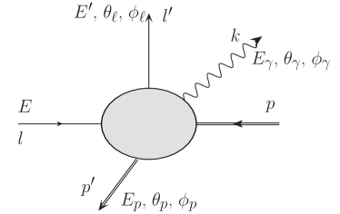
Figure 1: Definition of kinematic variables for lepton nucleon scattering.

At lowest order, lepton nucleon scattering is described by the exchange of a virtual photon. The spin-averaged matrix element of the electromagnetic current for a spin-1/2 nucleon, $e\bar{u}(p^{\prime})\Gamma^{\mu}_{p}u(p)$, can be decomposed into Dirac and Pauli form factors, $F_{1}^{p}$ and $F_{2}^{p}$, which are functions of the momentum transfer $Q^{2}=-(p-p^{\prime})^{2}$. They are normalized by $F_{1}^{p}(0)=1$ and $F_{1}^{p}(0)=\kappa_{p}-1$ with $\kappa_{p}=2.7928$ the proton’s magnetic moment in units of the nuclear magneton. The proton vertex is determined by

$$\Gamma^{\mu}_{p}=\gamma^{\mu}(F_{1}^{p}(Q^{2})+F_{2}^{p}(Q^{2}))-\frac{(p+p^{\prime})^{\mu}}{2M}F_{2}^{p}(Q^{2})$$ (1)

where $M$ is the nucleon mass. From this vertex rule one obtains the tree-level cross section for the scattering of unpolarized leptons with mass $m_{\ell}$ off unpolarized nucleons:

$$\frac{\mathrm{d}\sigma^{(0)}}{\mathrm{d}Q^{2}} = \frac{\pi\alpha^{2}}{Q^{4}\left((s-m_{\ell}^{2}-M^{2})^{2}-m_{\ell}^{2}M^{2}\right)}$$

$$\Bigl{[}2\left(F_{1}^{p}\right)^{2}\left((s-m_{\ell}^{2}-M^{2})^{2}+(s-Q^{2})^{2}-2s(m_{\ell}^{2}+M^{2})+(M^{2}+m_{\ell}^{2})^{2}\right)$$

$$+4F_{1}^{p}F_{2}^{p}Q^{2}\left(Q^{2}-2m_{\ell}^{2}\right)$$

$$+\left(F_{2}^{p}\right)^{2}\frac{Q^{2}}{M^{2}}\left((s-m_{\ell}^{2}-M^{2})(s-Q^{2})-(s-Q^{2})M^{2}-sm_{\ell}^{2}+(M^{2}-m_{\ell}^{2})^{2}\right)\Bigr{]}\,.$$

(see [27]). Here, $s$ is the square of the energy in the center-of-mass reference frame, $s=(l+p)^{2}$ and $\alpha$ the fine structure constant. An alternative compact expression for the Born cross section including all mass terms is given in App. A.

For electron scattering it is often a very good approximation to neglect the lepton mass. For the applications we have in mind, the energies of the incoming and scattered electrons, $E$ and $E^{\prime}$, are large, $E,E^{\prime}\gg m_{\ell}$. For not too small lepton scattering angles $\theta_{\ell}$ one can also assume that $m_{\ell}^{2}\ll Q^{2}$. It is also often convenient to use the Sachs electric and magnetic form factors $G_{E}=F_{1}^{p}-\tau F_{2}^{p}$ and $G_{M}=F_{1}^{p}+F_{2}^{p}$ with $\tau=Q^{2}/(4M^{2})$ and the cross section can be written in the more compact form, neglecting terms with the lepton mass,

$$\frac{\mathrm{d}\sigma^{(0)}}{\mathrm{d}\Omega_{\ell}}=\frac{\mathrm{d}\sigma_{\text{Mott}}}{\mathrm{d}\Omega_{\ell}}\frac{1}{\epsilon(1+\tau)}\left[\epsilon G_{E}^{2}(Q^{2})+\tau G_{M}^{2}(Q^{2})\right]$$ (3)

with

$$\frac{\mathrm{d}\sigma_{\text{Mott}}}{\mathrm{d}\Omega_{\ell}}=\frac{\alpha^{2}}{4E^{2}}\frac{\cos^{2}(\theta_{\ell}/2)}{\sin^{4}(\theta_{\ell}/2)}\frac{E^{\prime}}{E}$$ (4)

and

$$\epsilon=\left[1+2(1+\tau)\tan^{2}(\theta_{\ell}/2)\right]^{-1}\,.$$ (5)

We note that our program for the numerical evaluation of cross sections includes all lepton mass terms and is applicable also for the case of muon scattering.

The proton form factors are considered as external input and have to be extracted from measurements. We have implemented 5 different types of parametrizations existing in the literature. This can be easily modified, if needed. All our results shown below are obtained with a simple dipole form factor parametrization, $G_{E}=\left(1+Q^{2}/\Lambda^{2}\right)^{-2}$ and $G_{M}=\kappa_{p}G_{E}$ with $\Lambda=0.71$ GeV².

At the tree-level and without the emission of a hard photon, the momentum transfer to the nucleon can be determined from the energy and scattering angle of the outgoing lepton. However, bremsstrahlung can lead to a shift of $Q^{2}$ and we have to distinguish the value determined from the scattered lepton from its true value transferred to the nucleon. To emphasize this fact, we use the additional symbol $Q_{\ell}^{2}$, defined by

$$Q_{\ell}^{2}=-(l-l^{\prime})^{2}\,.$$ (6)

Higher-order corrections are due to additional photon emission and absorption, either virtual, described by loop diagrams, or real, described by bremsstrahlung diagrams. Both parts contain infrared (IR) divergences which cancel when combined. In our approach we use the phase-space slicing method to separate soft-photon radiation from hard-photon contributions. The separation is implemented by using a cut-off $\Delta$ for the energy of a radiated photon. $\Delta$ is chosen small, below the detection threshold for the observation of a photon in the detector, and the soft-photon part combined with loop diagrams is called non-radiative. First-order corrections, at order $\mathcal{O}(\alpha)$ relative to the Born cross section, are written as

$$\sigma^{(1)}=\sigma^{(1)}_{\text{non-rad}}+\sigma^{(1)}_{1h\gamma}\,,$$ (7)

and

$$\sigma^{(1)}_{\text{non-rad}}=\sigma^{(1)}_{1-\text{loop}}+\sigma^{(1)}_{1s\gamma}\,.$$ (8)

At second relative order, one has to include contributions with both one or two radiated photons and one has to distinguish the cases where only one or both photons are either soft or hard. The second-order contribution to the cross section, $\sigma^{(2)}$ is therefore split into three parts:

$$\sigma^{(2)}=\sigma^{(2)}_{\text{non-rad}}+\sigma^{(2)}_{1h\gamma}+\sigma^{(2)}_{2h\gamma},$$ (9)

where

$$\sigma^{(2)}_{\text{non-rad}}=\sigma^{(2)}_{2-\text{loop}}+\sigma^{(2)}_{1-\text{loop}+1s\gamma}+\sigma^{(2)}_{2s\gamma}\,,\quad\quad\sigma^{(2)}_{1h\gamma}=\sigma^{(2)}_{1-\text{loop}+1h\gamma}+\sigma^{(2)}_{1s\gamma+1h\gamma}\,.$$ (10)

The non-radiative parts are rendered IR-finite by including loop diagrams: $\sigma^{(2)}_{\text{non-rad}}$ contains two-loop contributions and mixed soft-photon + one-loop parts, while $\sigma^{(2)}_{1h\gamma}$ contains one-loop corrections to the radiative process with one hard photon.

In addition we will use correction factors defined relative to the differential Born-level cross section $\mathrm{d}\sigma^{(0)}$,

$$\sigma^{(1)}_{\text{non-rad}}=\int\mathrm{d}\sigma^{(0)}\Big{[}\delta^{(1)}_{1-\text{loop}}+\delta^{(1)}_{1s\gamma}(\Delta)\Big{]},$$ (11)

$$\sigma^{(2)}_{\text{non-rad}}=\int\mathrm{d}\sigma^{(0)}\Big{[}\delta^{(2)}_{2-\text{loop}}+\delta^{(2)}_{1-\text{loop}+1s\gamma}(\Delta)+\delta^{(2)}_{2s\gamma}(\Delta)\Big{]},$$ (12)

where each $\delta$ is labeled with indices as described above for the total cross sections. We also show explicitly the dependence of the soft-photon parts on the IR cut-off $\Delta$. The soft-photon part can be calculated analytically, integrating up to the cut-off $\Delta$, by using a soft-photon approximation as described in Sec. 4.1

Contributions with a hard photon, i.e. with energy above the cut-off $\Delta$, are infrared finite and the phase space integration can be performed numerically. For one hard photon at tree level, we can write

$$\sigma^{(1)}_{1h\gamma}=\int_{E_{\gamma}>\Delta}\mathrm{d}^{4}\sigma^{(1)}_{1\gamma}\,,$$ (13)

while at second order we define relative correction factors for the one-loop and soft photon contributions by writing

$$\sigma^{(2)}_{1h\gamma}=\int_{E_{\gamma}>\Delta}\mathrm{d}^{4}\sigma^{(1)}_{1\gamma}\left[\delta^{(1)}_{1-\text{loop}+1h\gamma}+\delta^{(1)}_{1s\gamma+1h\gamma}(\Delta)\right]\,,$$ (14)

where $\mathrm{d}^{4}\sigma^{(1)}_{1\gamma}$ is the differential cross section for one radiated hard photon at the tree-level. The calculation of $\sigma^{(2)}_{1h\gamma}$ is treated in Sec. 4.2. Finally, the cross section for two hard photons is given by

$$\sigma^{(2)}_{2h\gamma}=\int_{E_{\gamma},\;E^{\prime}_{\gamma}>\Delta}\mathrm{d}^{7}\sigma^{(2)}_{2\gamma}\,.$$ (15)

It is free of any infra-red singularities and can be calculated numerically as described in section 4.4. We emphasize that the cut-off parameter $\Delta$ is introduced only for a technical reason: it allows us to separate the IR singularities. Only separate parts contributing to the cross section carry a $\Delta$-dependence as shown in the formulas given above. The sum of non-radiative and hard-photon contributions has to be independent of $\Delta$. However, when we use the soft-photon approximation to calculate the non-radiative contributions, and due to numerical uncertainties we don’t expect the result to be exactly $\Delta$-independent. We will study this at more detail below.

Explicit simple expressions for Feynman diagrams with loops can be found in the literature. Where necessary, we use the Mathematica package Feyncalc [28] to perform the calculations, including a reduction to the conventional scalar one-loop Passarino-Veltman integrals $B_{0}$, $C_{0}$ and $D_{0}$. The final result is obtained in terms of scalar integrals and kinematic invariants. Where possible we use explicit simple expressions for the scalar integrals. For the numerical evaluation of more complex scalar integrals we use the package LoopTools [29].

3 First-order corrections

3.1 Non-radiative cross section

3.1.1 One-loop corrections

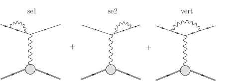
Figure 2: Feynman diagrams for the one-loop corrections at the lepton line.

The one-loop corrections at the lepton line include self energy diagrams at the external lines and the vertex graph. The first-order correction to the matrix element squared is given by

$$\left|\mathcal{M}_{\text{Born}}\right|^{2}+2\real(\mathcal{M}_{\text{Born}}^{\dagger}\mathcal{M}_{\text{se1+se2}})+2\real(\mathcal{M}_{\text{Born}}^{\dagger}\mathcal{M}_{\text{vert}})$$ (16)

where the meaning of the labels for the separate contributions corresponds to the diagrams shown in Fig. 2. The free lepton propagator for a lepton with four-momentum $l$, $S^{(0)}(l)$ is modified by the self-energy $\Sigma(l)$,

$$S(l)=S^{(0)}(l)+S^{(0)}(l)\Sigma(l)S(l).$$ (17)

The renormalized self-energy is given by

$$\Sigma^{R}(l)=\Sigma(l)-(\not{l}-m_{\ell})\delta Z_{2}-\delta m_{\ell},$$ (18)

where the counter-terms $\delta Z_{2}$ and $\delta m_{\ell}$ contain the ultra-violet (UV) divergences and are given, in dimensional regularisation, by

$$\delta Z_{2} =-\frac{\alpha}{4\pi}\left(\Delta_{\epsilon}-\log\frac{m_{\ell}^{2}}{\mu^{2}}+2\log\frac{\lambda^{2}}{m_{\ell}^{2}}+4\right),$$ (19)

$$\delta m_{\ell} =\frac{\alpha}{4\pi}m_{\ell}\left(3\Delta_{\epsilon}-3\log\frac{m_{\ell}^{2}}{\mu^{2}}+4\right).$$ (20)

$\Delta_{\epsilon}=\frac{2}{\epsilon}-\gamma_{E}+\log 4\pi$ contains the $1/\epsilon$-poles of the UV divergences, $\mu$ is the mass scale parameter of dimensional regularization and $\lambda$ is a finite photon-mass used to regularize the IR divergence. For on-shell leptons, the self-energy diagrams vanish after renormalization and we only need to include the vertex diagram. The relative one-loop correction is given by

$$\delta^{(1)}_{1-\text{loop}}=\frac{2\real(\mathcal{M}_{\text{Born}}^{\dagger}\mathcal{M}_{\text{vert}})}{\left|\mathcal{M}_{\text{Born}}\right|^{2}}.$$ (21)

For on-shell leptons, the vertex correction can be separated into two form factors, similar to the case of the photon-nucleon form factors. Therefore the correction can be taken into account by replacing the tree-level on-shell vertex by

$$\gamma^{\mu}\rightarrow\Gamma^{\mu}_{\text{vert}}\equiv F^{\ell}_{1}(Q_{\ell}^{2})\gamma^{\mu}+\frac{i}{2m_{\ell}}\sigma_{\mu\nu}q^{\nu}F^{\ell}_{2}(Q_{\ell}^{2})\,.$$ (22)

$F^{\ell}_{2}$ is UV and IR finite. It is proportional to $m_{\ell}$ and therefore very small, but we include it for completeness in our calculations. $F^{\ell}_{1}$ is both UV and IR divergent. The UV divergence is regularized using dimensional regularization and removed by renormalization. At first order the renormalized form factor is given by

$${F^{\ell}_{1}}^{(1,R)}(Q_{\ell}^{2})={F^{\ell}_{1}}^{(1)}(Q_{\ell}^{2})-{F^{\ell}_{1}}^{(1)}(0)={F^{\ell}_{1}}^{(1)}(Q_{\ell}^{2})+\delta Z_{1}\,,$$ (23)

where we introduced additional upper indices to display the loop-order and distinguish renormalized (with index $R$) from unrenormalized quantities. The counter-term $\delta Z_{1}$ is given in the $\overline{\text{MS}}$ prescription by

$$\delta Z_{1}=-\frac{\alpha}{4\pi}\left(\Delta_{\epsilon}-\log\frac{m_{\ell}^{2}}{\mu^{2}}+2\log\frac{\lambda^{2}}{m_{\ell}^{2}}+4\right)\,.$$ (24)

$\delta Z_{1}$ is identical with $\delta Z_{2}$, Eq. (19), as a consequence of the Ward identity. The relative vertex correction is therefore given by, up to terms suppressed by the lepton mass,

$$\delta^{(1)}_{1-\text{loop}}=2{F^{\ell}_{1}}^{(1,R)}\,.$$ (25)

The result of the loop integration is well-known and can be obtained including the exact lepton mass dependence:

$$\begin{split}\delta^{(1)}_{1-\text{loop}}&=\frac{\alpha}{\pi}\Bigg{[}\frac{v^{2}+1}{4v}\ln\left(\frac{v+1}{v-1}\right)\ln\left(\frac{v^{2}-1}{4v^{2}}\right)+\frac{2v^{2}+1}{2v}\ln\left(\frac{v+1}{v-1}\right)-2\\ &+\frac{v^{2}+1}{2v}\left(\textrm{Li}_{2}\left(\frac{v+1}{2v}\right)-\textrm{Li}_{2}\left(\frac{v-1}{2v}\right)\right)\Bigg{]}+\delta_{\text{IR}},\end{split}$$ (26)

where $v=\sqrt{1+4m_{\ell}^{2}/Q_{\ell}^{2}}$ and $\delta_{\text{IR}}$ is the term that contains the IR divergence, given by

$$\delta_{\text{IR}}=\frac{\alpha}{\pi}\ln(\frac{\lambda^{2}}{m_{\ell}^{2}})\left[\frac{v^{2}+1}{2v}\ln(\frac{v+1}{v-1})-1\right]\,.$$ (27)

This term will cancel at the level of the cross section when one-photon radiation is included, as will be seen below.

Although in most cases it is safe to ignore the $F^{\ell}_{2}$ form factor, we include it in our calculation, since it might become important in some regions of the phase space or for the case of $\mu$ scattering. The expression for this form factor can be found in [30] and is given, at first order, by

$${F^{\ell}_{2}}^{(1)}=\frac{\alpha}{4\pi}\frac{v^{2}-1}{v}\ln(\frac{v+1}{v-1})\,.$$ (28)

3.1.2 One radiated photon in the soft-photon approximation

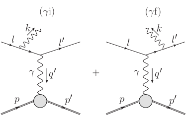
Figure 3: Feynman diagrams for first-order bremsstrahlung corrections.

The diagrams that contribute to the radiative process $\ell p\rightarrow\ell p\gamma$ are shown in Fig. 3. We indicate by labels i and f when the photon is emitted from the initial or the final lepton. The 4-momentum of the additional photon is denoted by $k^{\mu}$ and its energy by $E_{\gamma}$. The matrix element for radiative scattering is

$$\mathcal{M}_{1\gamma}=\mathcal{M}_{1\gamma\text{i}}+\mathcal{M}_{1\gamma\text{f}}\,.$$ (29)

Note that the momentum transfer is shifted by the emission of a photon, $q^{\mu}\rightarrow q^{\prime\mu}=l^{\mu}-l^{\prime\mu}-k^{\mu}$, and the matrix element is proportional to $1/Q^{2}$, not $1/Q^{2}_{\ell}$. In the soft-photon approximation, the matrix element reduces to

$$\mathcal{M}_{1\gamma}\rightarrow\mathcal{M}_{1s\gamma}=-e\mathcal{M}_{0\gamma}\left(\frac{l\epsilon^{*}}{lk}-\frac{l^{\prime}\epsilon^{*}}{l^{\prime}k}\right)$$ (30)

where $\epsilon^{\mu}$ is the photon polarization vector. Integration over the photon 4-momentum up to a cut-off $\Delta$ in the soft-photon approximation leads to

$$\int_{E_{\gamma}<\Delta}\mathrm{d}^{4}\sigma_{1s\gamma}^{(1)}=\mathrm{d}\sigma^{(0)}\left(-\frac{\alpha}{2\pi^{2}}\right)\int_{E_{\gamma}<\Delta}\frac{\mathrm{d}^{3}k}{2E_{\gamma}}\left(\frac{l}{lk}-\frac{l^{\prime}}{l^{\prime}k}\right)^{2}.$$ (31)

Then the relative one soft-photon correction is given by

$$\delta^{(1)}_{1s\gamma}(\Delta)=\left(-\frac{\alpha}{2\pi^{2}}\right)\int_{E_{\gamma}<\Delta}\frac{\mathrm{d}^{3}k}{2E_{\gamma}}\left(\frac{l}{lk}-\frac{l^{\prime}}{l^{\prime}k}\right)^{2}=-\frac{\alpha}{\pi}\left(B_{ll}-B_{ll^{\prime}}+B_{l^{\prime}l^{\prime}}\right)-\delta_{\text{IR}}\,,$$ (32)

where the result has been written as a contribution from initial state radiation, $B_{ll}$, final state radiation, $B_{l^{\prime}l^{\prime}}$ and the interference between the two, $B_{ll^{\prime}}$. The IR divergence is contained in $\delta_{\text{IR}}$ and cancels exactly against the IR divergent part of Eq. (26). The calculation of $B_{ll}$ and $B_{l^{\prime}l^{\prime}}$ is straightforward and leads to

$$B_{ll} =\ln\left(\frac{2\Delta}{m_{\ell}}\right)+\frac{E}{|\vec{l}|}\ln\left(\frac{m_{\ell}}{E+|\vec{l}|}\right)\,,$$ (33)

$$B_{l^{\prime}l^{\prime}} =\ln\left(\frac{2\Delta}{m_{\ell}}\right)+\frac{E^{\prime}}{|\vec{l}^{\prime}|}\ln\left(\frac{m_{\ell}}{E^{\prime}+|\vec{l}^{\prime}|}\right)\,.$$ (34)

The calculation of the interference term $B_{ll^{\prime}}$ is more involved and can be done following Refs. [32] and [8]. The final result is given by

$$B_{ll^{\prime}} =\ln(\frac{4\Delta^{2}}{m_{\ell}^{2}})\frac{v^{2}+1}{v}\ln(\frac{v+1}{v-1})+\frac{\beta ll^{\prime}}{\xi(\beta E-E^{\prime})}\Bigg{[}\ln^{2}\left(\frac{E-|\vec{l}|}{E+|\vec{l}|}\right)-\ln^{2}\left(\frac{E^{\prime}-|\vec{l}^{\prime}|}{E^{\prime}+|\vec{l^{\prime}}|}\right)$$

$$+\textrm{Li}_{2}\left(1-\frac{\beta(E-|\vec{l}|)}{\xi}\right)-\textrm{Li}_{2}\left(1-\frac{\beta(E^{\prime}-|\vec{l}^{\prime}|)}{\xi}\right)$$ (35)

$$+\textrm{Li}_{2}\left(1-\frac{\beta(E+|\vec{l}|)}{\xi}\right)-\textrm{Li}_{2}\left(1-\frac{\beta(E^{\prime}+|\vec{l}^{\prime}|)}{\xi}\right)\Bigg{]}\,,$$

where $ll^{\prime}=m_{\ell}^{2}+Q^{2}_{\ell}/2$ is the product of the 4-momenta of the incident and scattered lepton. The following abbreviations have been used:

$$\beta=\frac{ll^{\prime}+\sqrt{(ll^{\prime})^{2}-m_{\ell}^{4}}}{m_{\ell}^{2}}\,,$$

$$\xi=\frac{\beta ll^{\prime}-m_{\ell}^{2}}{\beta E-E^{\prime}}\,.$$

The non-radiative relative correction at first order for the cross section with no observed photon is IR finite and is given by

$$\delta^{(1)}_{\text{non-rad}}(\Delta)=\delta^{(1)}_{1-\text{loop}}+\delta^{(1)}_{1s\gamma}(\Delta)\,.$$ (36)

3.2 One hard photon cross section

The cross-section for the radiative process with one hard photon is given by

$$\mathrm{d}^{4}\sigma^{(1)}_{1h\gamma}=\frac{\mathrm{d}^{4}\Gamma_{1\gamma}}{4M|\vec{l}\,|}\overline{|\mathcal{M}_{1\gamma}|^{2}}$$ (37)

where the flux factor is given for the fixed-target frame and the bar indicates that one has to average and sum over the polarization degrees of freedom in the initial and final state, respectively. The differential phase-space is given by

$$\mathrm{d}^{4}\Gamma_{1\gamma}= \int\frac{1}{(2\pi)^{5}}\,\mathrm{d}^{4}l^{\prime}\,\mathrm{d}^{4}k\,\mathrm{d}^{4}p^{\prime}\,\delta(l^{\prime\,2}-m_{\ell}^{2})\delta(k^{2})\delta(p^{\prime\,2}-M^{2})\delta^{4}\left(l+p-l^{\prime}-p^{\prime}-k\right)\,.$$

We can choose a phase space parametrization in terms of energies and polar angles of the lepton and photon in the final state as described in detail in App. B. Using the notation defined there, the cross-section for one hard radiated photon becomes

$$\sigma^{(1)}_{1h\gamma} =\frac{1}{32(2\pi)^{4}M|\vec{l}\,|}\int\limits_{E^{\prime}_{\text{min}}}^{E^{\prime}_{\text{max}}}\mathrm{d}E^{\prime}\int\limits_{\theta_{\ell}^{\text{min}}}^{\theta_{\ell}^{\text{max}}}\mathrm{d}\cos\theta_{\ell}\int\limits_{\Delta}^{E_{\gamma}^{\text{max}}}\mathrm{d}E_{\gamma}\int\limits_{\theta_{\gamma}^{\text{min}}}^{\theta_{\gamma}^{\text{max}}}\mathrm{d}\cos\theta_{\gamma}$$

$$\times\frac{\overline{|\mathcal{M}_{1\gamma}|^{2}}}{\sin\theta_{\ell}\sin\theta_{\gamma}\sin\phi_{\gamma}}\Theta\left(1-\frac{A^{2}}{B^{2}}\right)\,,$$ (38)

where $\sin\phi_{\gamma}=\sqrt{1-A^{2}/B^{2}}$. Explicit expressions for $A=A(E^{\prime},\theta_{\ell},E_{\gamma},\theta_{\gamma})$, $B=B(E^{\prime},\theta_{\ell},E_{\gamma},\theta_{\gamma})$ and the integration limits are given in App. B, see Eqs. (72) and (75). The matrix element squared is calculated with the help of the Feyncalc package and the final result is expressed in terms of invariant products of 4-momenta. A compact expression is given in App. A. We perform the numerical integration with the Cuba package [34].

3.3 Vacuum polarization

The vacuum polarization, re-summed to all orders, leads to the replacement of the photon propagator, in Feynman gauge, by

$$G_{\mu\nu}=\frac{-ig_{\mu\nu}}{q^{2}\left[1-\Pi(q^{2})\right]}\,.$$ (39)

The correction can be absorbed in the fine-structure constant

$$\alpha_{\text{eff}}(q^{2})=\frac{\alpha}{1-\Pi(q^{2})}.$$ (40)

The contribution from lepton loops is given at first order by

$$\delta_{\text{vac-pol}}^{\text{leptons}}=2\Pi_{e+\mu+\tau}(q^{2})=\delta_{\text{vac-pol}}^{e}+\delta_{\text{vac-pol}}^{\mu}+\delta_{\text{vac-pol}}^{\tau}$$ (41)

and can be written, for space-like momentum transfer $-q^{2}=Q^{2}>0$, in the compact form

$$\delta_{\text{vac-pol}}^{\ell}=\frac{2\alpha}{3\pi}\left[\left(v^{2}-\frac{8}{3}\right)+v\frac{(3-v^{2})}{2}\ln\left(\frac{v+1}{v-1}\right)\right],$$ (42)

where $v=\sqrt{1+4m_{\ell}^{2}/Q^{2}}$ with $m_{\ell}$ the mass of the lepton in the loop. At large $Q^{2}$ and including the two-loop contribution, one may use [35]:

$$\delta_{\text{vac-pol}}^{\ell}=2\frac{\alpha}{\pi}\left(\frac{1}{3}\ln\frac{Q^{2}}{m_{\ell}^{2}}-\frac{5}{9}\right)+2\left(\frac{\alpha}{\pi}\right)^{2}\left(\frac{1}{4}\ln\frac{Q^{2}}{m_{\ell}^{2}}+\zeta(3)-\frac{5}{24}\right)+O(\alpha^{3})\,.$$ (43)

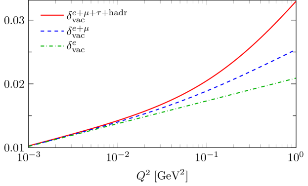
Figure 4: Leptonic and hadronic contributions to the vacuum polarization in the $Q^{2}$ range relevant for the P2 experiment.

The hadronic part of $\Pi(q^{2})$ can be extracted from experimental data for the cross section of $e^{+}e^{-}$ annihilation into hadrons. We use a table provided by F. Ignatov [36] (see also [37]) but it is straightforward to replace this by other parametrisations, as for example the one of Ref. [38] or [39]. In Fig. 4 we show numerical results for $\delta_{\text{vac-pol}}$. We conclude that one has to include the vacuum polarisation effect in a high-precision calculation of the cross section and contributions from other than electron loops should not be neglected for $Q^{2}$ values above a few times $10^{-2}$ GeV².

4 Second-order corrections

4.1 Non-radiative corrections

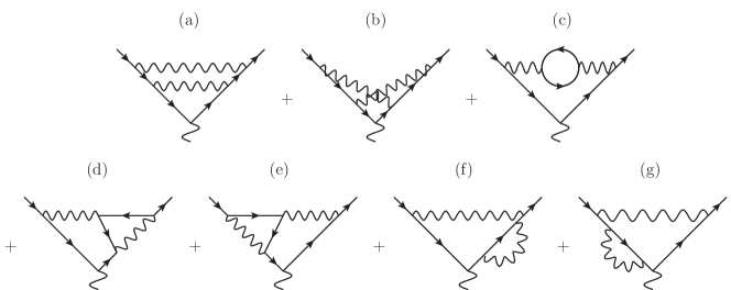
Figure 5: Feynman diagrams for two-loop vertex corrections.

The Feynman diagrams for two-loop corrections at the lepton line are shown in Fig. 5. Their contribution to the matrix element is denoted by $\mathcal{M}_{\text{2-loop}}$. The relative two-loop correction factor includes the square of the one-loop corrections and is given by

$$\delta^{(2)}_{2-\text{loop}}=\frac{\left|\mathcal{M}_{\text{vert}}\right|^{2}+2\real(\mathcal{M}_{\text{Born}}^{\dagger}\mathcal{M}_{\text{2-loop}})}{\left|\mathcal{M}_{\text{Born}}\right|^{2}}\,.$$ (44)

For electron scattering, the Pauli form factor $F_{2}^{\ell}$ can be neglected at this order. Then the two-loop correction reduces to

$$\delta^{(2)}_{2-\text{loop}}=\left(F_{1}^{\ell(1)}\right)^{2}+2F_{1}^{\ell(2)}.$$ (45)

A compact expression for $\delta^{(2)}_{2-\text{loop}}$, valid for $Q_{\ell}^{2}\gg m_{\ell}^{2}$, can be extracted from Ref. [40] and is given by

$$\delta^{(2)}_{2-\text{loop}}= \frac{1}{2}\left(\delta_{\text{1-\text{loop}}}^{(1)}\right)^{2}+\left(\frac{\alpha}{4\pi}\right)^{2}\Bigg{[}-\frac{8}{9}L^{3}+\frac{76}{9}L^{2}+\left(-\frac{979}{27}-\frac{44\pi^{2}}{9}+48\zeta(3)\right)L+\frac{4252}{27}$$

$$+\frac{47\pi^{2}}{3}-16\pi^{2}\ln(2)-72\zeta(3)-\frac{64\pi^{4}}{45}+\mathcal{O}\left(\frac{m_{\ell}^{2}}{Q_{\ell}^{2}}\right)\Bigg{]}\,,$$ (46)

where $L=\ln(Q_{\ell}^{2}/m_{\ell}^{2})$. Eq. (46) agrees with the earlier calculation of Ref. [43]. After removing the UV divergent parts the expression still contains IR divergences which cancel when soft-photon corrections are included at the level of the cross section. The soft-photon corrections at second order are corrections from two-soft-photon radiation and one-loop corrections for one-soft-photon radiation.

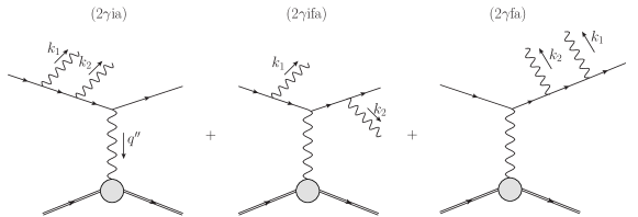
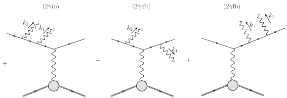
Figure 6: Feynman diagrams for two-photon bremsstrahlung.

The diagrams for two-photon radiation are shown in Fig. 6. In the soft-photon approximation, the corresponding correction factor is given by

$$\delta^{(2)}_{2s\gamma}=\frac{1}{2!}\left(-\frac{\alpha}{4\pi^{2}}\right)^{2}\int_{E_{\gamma},\;E^{\prime}_{\gamma}<\Delta}\frac{\mathrm{d}^{3}k_{1}}{E_{\gamma}}\frac{\mathrm{d}^{3}k_{2}}{E^{\prime}_{\gamma}}\left(\frac{l_{1}}{l_{1}k_{1}}-\frac{l_{2}}{l_{2}k_{1}}\right)^{2}\left(\frac{l_{1}}{l_{1}k_{2}}-\frac{l_{2}}{l_{2}k_{2}}\right)^{2}\,.$$ (47)

If both photon energies separately are taken smaller than the cut-off value $\Delta$, as we assume here, the phase space integration factorizes and leads to

$$\delta^{(2)}_{2s\gamma}=\frac{1}{2!}\left(\delta^{(1)}_{1s\gamma}\right)^{2}\,.$$ (48)

In contrast, if the integration is done by restricting the total unobserved energy, i.e., using $E_{\gamma}+E^{\prime}_{\gamma}<\Delta$, as was done for example in [40], the soft-photon correction factor $\delta^{(2)}_{2s\gamma}$ contains an additional term $-\frac{\alpha^{2}}{3}(L-1)^{2}$, which comes from the phase-space overlap of the two photons [14]. In our approach we take account of this overlap region in the contribution from two hard photons. Of course, the final result has to be independent of the way the phase-space slicing is implemented.

The Feynman diagrams for one radiated photon at one-loop order are shown in Fig. 7. When treating the photon as soft, one can approximate their contribution by a factorized form in terms of the one-photon and one-loop correction factors:

$$\delta^{(2)}_{1-\text{loop}+1s\gamma}(\Delta)=\delta_{1-\text{loop}}^{(1)}\delta_{1s\gamma}^{(1)}(\Delta)\,.$$ (49)

Combining all non-radiative second order corrections at the level of the cross section we obtain an IR finite, but cut-off dependent result,

$$\delta^{(2)}_{\text{non-rad}}(\Delta)=\delta^{(2)}_{2-\text{loop}}+\delta^{(1)}_{1-\text{loop}}\delta^{(1)}_{1s\gamma}(\Delta)+\delta^{(2)}_{2s\gamma}(\Delta)\,.$$ (50)

4.2 One-loop corrections to radiative scattering

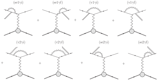
Figure 7: Feynman diagrams for one-loop corrections to one-photon bremsstrahlung.

A complete second-order calculation of the cross section includes one-loop corrections for the process with one radiated photon. The corresponding Feynman diagrams are shown in Fig. 7. Lepton self energy corrections at external legs are not needed since their contribution vanishes after renormalization as mentioned above.

First, there are two self-energy diagrams with a photon radiated from the off-shell line. Their contribution to the matrix element is denoted by

$$\mathcal{M}_{\text{se1}\gamma}=\mathcal{M}_{\text{se1}\gamma\text{i}}+\mathcal{M}_{\text{se1}\gamma\text{f}}\,.$$ (51)

The one-loop integral entering $\mathcal{M}_{\text{se1}\gamma}$ is IR finite. Its UV divergence is removed by adding the vertex counter-term proportional to $\delta Z_{1}$ (see Eq. (24)).

Next, two diagrams are vertex corrections with a photon emitted from the off-shell line and their matrix element is denoted by

$$\mathcal{M}_{\text{v1}\gamma}=\mathcal{M}_{\text{v1}\gamma\text{i}}+\mathcal{M}_{\text{v1}\gamma\text{f}}\,.$$ (52)

The 4-point one-loop integrals needed here are UV finite, but contain IR-divergent contributions.

The second row of diagrams in Fig. 7 have a photon attached to an external, on-shell lepton line; two of them are self energy insertions in the off-shell lepton line,

$$\mathcal{M}_{\text{se2}\gamma}=\mathcal{M}_{\text{se2}\gamma\text{i}}+\mathcal{M}_{\text{se2}\gamma\text{f}}\,,$$ (53)

and two of them describe a one-loop vertex correction,

$$\mathcal{M}_{\text{v2}\gamma}=\mathcal{M}_{\text{v2}\gamma\text{i}}+\mathcal{M}_{\text{v2}\gamma\text{f}}\,.$$ (54)

These diagrams are UV divergent and require renormalization by including counter-terms, either at the vertex ($\delta Z_{1}$) or at the lepton self energy ($\delta Z_{2}$ and $\delta m_{\ell}$).

The second-order corrections due to these diagrams are obtained from the interference with the first-order diagrams. They can be split into parts,

$$\delta^{(2)}_{1-\text{loop}+1h\gamma}=\delta_{\text{se1}\gamma}+\delta_{\text{v1}\gamma}+\delta_{\text{se2}\gamma}+\delta_{\text{v2}\gamma}\,,$$ (55)

with an obvious meaning of the indices as explained above.

4.3 One hard and one soft photon

IR divergences contained in one-loop corrections to the radiative process described in the previous sub-section are cancelled by corresponding IR divergences from soft-photon contributions of 2-photon bremsstrahlung. The diagrams for $\ell p\rightarrow\ell p\gamma\gamma$ have been presented above in Fig. 6. We separate IR divergent contributions by assuming one photon is soft and the other is hard. In the soft-photon approximation, the IR divergence can be factorized as described above. If the soft photon has momentum $k_{1}$, the IR part of $\mathcal{M}_{2\gamma}$ is contained in

$$\mathcal{M}_{2\gamma}^{\text{IR-div}}=-e\mathcal{M}_{1\gamma}(k_{2})\left(\frac{l\epsilon^{*}}{lk_{1}}-\frac{l^{\prime}\epsilon^{*}}{l^{\prime}k_{1}}\right)\,,$$ (56)

where $\mathcal{M}_{1\gamma}(k_{2})$ is the matrix element for bremsstrahlung of a photon with momentum $k_{2}$. Of course, one has to include a similar term with interchanged photon momenta $k_{1}\leftrightarrow k_{2}$.

The cross section for two photons in the final state is given by

$$\mathrm{d}^{7}\sigma_{2\gamma}=\frac{\mathrm{d}^{7}\Gamma_{2\gamma}}{2\cdot 4M|\vec{l}|}\overline{|\mathcal{M}_{2\gamma}|^{2}}\,,$$ (57)

where a symmetrization factor of one-half is applied to take into account the fact that there are two identical particles in the final state. Making the integration over the photon energies explicit and taking into account that the cross section is symmetric with respect to interchanging $k_{1}\leftrightarrow k_{2}$, the separation between soft- and hard-photon phase space regions is done as

$$\int_{0}^{E_{\gamma}^{\text{max}}}\mathrm{d}E_{\gamma}\int_{0}^{E_{\gamma}^{\text{max}}}\mathrm{d}E_{\gamma}^{\prime}=\int_{0}^{\Delta}\mathrm{d}E_{\gamma}\int_{0}^{\Delta}\mathrm{d}E_{\gamma}^{\prime}+2\int_{\Delta}^{E_{\gamma}^{\text{max}}}\mathrm{d}E_{\gamma}\int_{0}^{\Delta}\mathrm{d}E_{\gamma}^{\prime}+\int_{\Delta}^{E_{\gamma}^{\text{max}}}\mathrm{d}E_{\gamma}\int_{\Delta}^{E_{\gamma}^{\text{max}}}\mathrm{d}E_{\gamma}^{\prime}\,.$$ (58)

Only the second term on the right-hand side of Eq. (58) contributes to the part of the total cross section considered here, where we require one hard and one soft photon. The first part is purely soft-photon and contributes to the non-radiative cross section, combined with the 2-loop contribution. The last term for two hard photons is described in the next sub-section.

The infrared divergence can be factorized, resulting in

$$\sigma^{(2)}_{1s\gamma+1h\gamma}(\Delta)=2\int_{\Delta}^{E_{\gamma}^{\text{m}ax}}\int_{0}^{\Delta}\left(\mathrm{d}^{7}\sigma_{2\gamma}\right)_{1\gamma\rightarrow 0}=\delta^{(1)}_{1s\gamma}(\Delta)\int_{\Delta}^{E_{\gamma}^{\text{m}ax}}\mathrm{d}^{4}\sigma_{1\gamma}+2\int_{\Delta}^{E_{\gamma}^{\text{m}ax}}\int_{0}^{\Delta}\left(\mathrm{d}^{7}\sigma_{2\gamma}\right)_{1\gamma\rightarrow 0}^{\text{IR-finite}},$$ (59)

where $\delta^{(1)}_{1s\gamma}(\Delta)$ was defined in Eq. (32) and the factor of 2 was cancelled by the symmetry factor of the 2-photon cross section. Its IR-divergent part cancels against corresponding parts of the one-loop corrections to radiative scattering. One can show that the factorized part (the first term of the right-hand side of Eq. (59)) emerges from those four Feynman diagrams of Fig. 6 where the soft photon is emitted from an on-shell line. The two remaining diagrams with a soft photon coming from an off-shell line lead to an IR-finite contribution (the last term in Eq. (59)). This part can be safely calculated by numerical methods.

4.4 Two hard-photons

The cross section for $\ell p\rightarrow\ell p\gamma\gamma$ is given by Eq. (57). The differential phase-space is given by

$$\mathrm{d}^{7}\Gamma= \int\frac{1}{(2\pi)^{8}}\,\mathrm{d}^{4}l^{\prime}\,\mathrm{d}^{4}p^{\prime}\,\mathrm{d}^{4}k_{1}\,\mathrm{d}^{4}k_{2}\,\delta(l^{\prime\,2}-m_{\ell}^{2})\delta(p^{\prime\,2}-M^{2})\delta(k_{1}^{2})\delta(k_{2}^{2})$$

$$\times\delta^{4}\left(l+p-l^{\prime}-p^{\prime}-k_{1}-k_{2}\right)\,.$$ (60)

The treatment of the delta-functions and the derivation of integration limits is described in App. C. The spin-averaged square of the matrix element is calculated with the Feyncalc package and expressed in terms of invariants. The result is lengthy and not given here. Using the notation defined in App. C, the cross section for two-hard-photon radiation is expressed as

$$\sigma^{(2)}_{2h\gamma} =\frac{E_{\gamma}E^{\prime}_{\gamma}|\vec{l}^{\,\prime}|}{128(2\pi)^{7}M|\vec{l}|}\int\limits_{E^{\prime}_{\text{min}}}^{E^{\prime}_{\text{max}}}\mathrm{d}E^{\prime}\int\limits_{\cos\theta_{\ell,\text{min}}}^{\cos\theta_{\ell,\text{max}}}\mathrm{d}\cos\theta_{\ell}\int\limits_{\Delta}^{E_{\gamma,\text{max}}}\mathrm{d}E_{\gamma}\int\limits_{\Delta}^{E^{\prime}_{\gamma,\text{max}}}\mathrm{d}E^{\prime}_{\gamma}$$ (61)

$$\times\int\limits_{\cos\theta^{\prime}_{\gamma,\text{min}}}^{\cos\theta^{\prime}_{\gamma,\text{max}}}\mathrm{d}\cos\theta^{\prime}_{\gamma}\int\limits_{\phi^{\prime}_{\gamma,\text{min}}}^{\phi^{\prime}_{\gamma,\text{max}}}\mathrm{d}\phi^{\prime}_{\gamma}\int\limits_{\cos\theta_{\gamma,\text{min}}}^{\cos\theta_{\gamma,\text{max}}}\mathrm{d}\cos\theta_{\gamma}\frac{\overline{|\mathcal{M}_{2\gamma}|^{2}}}{\left|\alpha_{1}\cos\phi_{\gamma}-\alpha_{2}\sin\phi_{\gamma}\right|}\Theta\left(1-\frac{\alpha_{3}^{2}}{\alpha_{1}^{2}+\alpha_{2}^{2}}\right)\,.$$

The integration limits and the definition of the quantities $\alpha_{i}$ are given in App. C. Since the IR poles are cut off by lower integration limits on the photon energies, one can, in principle use standard integration packages for numerical calculations. It turns out, however, that collinear poles in the differential cross section render a naive approach numerically unstable. In order to deal with this problem we have used a partial fractioning to separate the collinear poles

$$\mathrm{d}^{7}\sigma^{(2)}_{2\gamma}\propto\frac{1}{(lk_{1})\cdot(lk_{2})\cdot(l^{\prime}k_{1})\cdot(l^{\prime}k_{2})}\rightarrow\frac{A}{lk_{1}}+\frac{B}{lk_{2}}+\frac{C}{l^{\prime}k_{1}}+\frac{D}{l^{\prime}k_{2}}\,.$$ (62)

For each term in the sum after partial fractioning we find a specific change of integration variables which allows us to obtain an efficient and numerically stable integration.

5 Numerical tests

The presence of divergences in intermediate results forces us to introduce various regularization parameters which must cancel in the final result:

• UV divergences are treated in dimensional regularization where pole terms in $\Delta_{\epsilon}$ appear. They are accompanied by logarithms of a mass scale parameter $\mu$ introduced to keep the mass dimension of loop integrals homogeneous. Both the $\Delta_{\epsilon}$- and $\mu$-dependence cancel by including corresponding counter-terms.

• IR divergences are regularized by a finite photon mass $\lambda$. Logarithms of the photon mass have to cancel exactly between loop contributions and corrections from soft-photon radiation.

• The phase space slicing parameter $\Delta$ was introduced to separate soft-photon from hard-photon contributions. The part with $E_{\gamma},E^{\prime}_{\gamma}<\Delta$ is calculated in the soft-photon approximation. Therefore the $\Delta$-dependence disappears only in the limit $\Delta\rightarrow 0$. A residual $\Delta$-dependence may be visible if $\Delta$ is chosen too large.

$\lambda^{2}$ [GeV2]	$m_{e}^{2}$	$10^{-4}$	$10^{-8}$	$10^{-12}$
$\sigma^{(2)}_{1h\gamma}$	$4034.10\pm 0.92$	$4033.33\pm 0.92$	$4033.89\pm 0.87$	$4033.79\pm 0.88$
$\Delta_{\epsilon}$	$0$	$10^{2}$	$10^{4}$	$10^{6}$
$\sigma^{(2)}_{1h\gamma}$	$4034.10\pm 0.92$	$4033.84\pm 0.91$	$4033.41\pm 0.90$	$4031.11\pm 0.92$
$\mu^{2}$	$1$	$10^{4}$	$10^{8}$	$10^{12}$
$\sigma^{(2)}_{1h\gamma}$	$4034.10\pm 0.92$	$4033.03\pm 0.90$	$4034.04\pm 0.94$	$4033.41\pm 0.92$

Table 1: Test of the independence of $\sigma^{(2)}_{1h\gamma}$ (see Eq. (14)) on the unphysical regularization parameters $\lambda^{2}$, $\Delta_{\epsilon}$ and $\mu^{2}$. The uncertainty estimates are due to the finite statistics of the Monte Carlo integration.

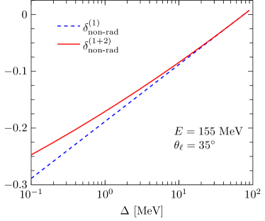
Figure 8: The dependence of the non-radiative parts of the correction factors at first and second order on the phase space slicing cut-off $\Delta$.

The implementation of loop integrals in the LoopTools package [29] allows us to keep the parameters $\Delta_{\epsilon}$, $\mu$ and $\lambda$ in separate parts of the calculation. Their cancellation can therefore be tested numerically. As an example, we show numerical results for the $O(\alpha)$ corrected one-photon bremsstrahlung cross section, given in Eq. (14) for P2 kinematics, i.e. for $E=155$ MeV, $\theta_{\ell}=35^{\circ}\pm 10^{\circ}$ and $E^{\prime}_{\text{min}}=45$ MeV and with a cut-off for the photon energy of $\Delta=10$ MeV. We take default values for the three regularization parameters as $\lambda^{2}=m_{e}^{2}$, $\Delta_{\epsilon}=0$ and $\mu^{2}=1$. From Tab. 1 we conclude that these unphysical parameters can be varied over a very large range of values without leading to a significant numerical variation of the correction factor. The observed behaviour constitutes a test of an important part of the calculation.

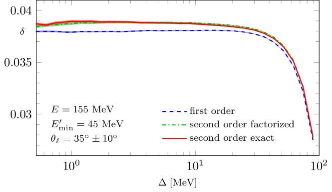
Figure 9: Test of the $\Delta$-independence of the complete correction factors when non-radiative contributions and hard-photon radiative effects are added, at first order $\delta=\sigma^{(1)}/\sigma^{(0)}-1$ and at second order $\delta=\sigma^{(2)}/\sigma^{(0)}-1$. Beam energy and the range of the scattering angle is chosen for the P2 experiment. The meaning of the labels “factorized” and “exact” is explained in the text.

The non-radiative parts of the cross section depend logarithmically on the phase space slicing parameter $\Delta$, at first order $\delta^{(1)}_{\text{non-rad}}\propto\ln\Delta$, at second order $\delta^{(2)}_{\text{non-rad}}\propto\ln^{2}\Delta$. A typical example of numerical results of the $\Delta$-dependence for the case of the P2 experiment is shown in Fig. 8. This $\Delta$-dependence is cancelled by the hard-photon contribution. In Fig. 9 we show an example, again for the kinematics of the P2 experiment. At large values of the soft-photon cut-off, when $\Delta$ reaches some 10 percent of the beam energy, the break-down of the soft-photon approximation is visible. Below $\Delta\simeq 10$ MeV, there is a nice plateau where the total result is independent of the cut-off. At first order, the cancellation looks perfect while for the second-order calculation one can observe that the numerical cancellation becomes less and less stable for decreasing $\Delta$. However, the choice $1~{}\text{MeV}\>\raisebox{-2.15277pt}{$\stackrel{{\scriptstyle\textstyle<}}{{\sim}}$}\>\Delta\>\raisebox{-2.15277pt}{$\stackrel{{\scriptstyle\textstyle<}}{{\sim}}$}\>10$ MeV is appropriate for the P2 experiment and guarantees that the soft-photon approximation used for the calculation of the non-radiative part of the total correction does not lead to a significant distortion of the total result.

It is also interesting to study an approximation for the calculation of $\delta^{(2)}_{1-\text{loop}+1h\gamma}$, Eq. (55). The approximation consists in assuming that the one hard-photon correction and the loop correction factorize also for finite values of the photon energy. This amounts to the replacement

$$\delta^{(2)}_{1-\text{loop}+1h\gamma}\rightarrow\delta^{(1)}_{1-\text{loop}}.$$ (63)

Figure 9 shows an example of numerical results based on this approximation (green, dash-dotted line). We find good agreement between the exact calculation and the approximation, at the level of $10^{-4}$ and better for the energy and angle range shown in this figure. In a more detailed study we found that the differences are largest in the vicinity of the final-state radiation peak.

6 Numerical results

We start this section with the discussion of a few numerical results for leptonic radiative corrections which are relevant for the P2 experiment at the MESA facility in Mainz [2]. The P2 experiment plans to measure the parity-violating asymmetry in elastic electron proton scattering with a polarized electron beam of energy $E=155$ MeV. The P2 spectrometer covers an angular acceptance range of $35\pm 10^{\circ}$ and for simplicity we assume that only scattered electrons with a fixed energy of at least $E^{\prime}_{\rm min}=45$ MeV are detected. The average momentum transfer squared is $\langle Q^{2}\rangle=6\cdot 10^{-3}$ GeV². An ancillary measurement for the determination of the axial and strange magnetic form factors at backward angles is also possible. Such a measurement could cover the angular range $135^{\circ}\leq\theta_{\ell}\leq 155^{\circ}$. We repeat that we have used a simple dipole parametrization for the proton form factors, $G_{E}=\left(1+Q^{2}/\Lambda^{2}\right)^{-2}$ and $G_{M}=\kappa_{p}G_{E}$ with $\Lambda=0.71$ GeV² and we have checked that, while the cross sections can change by a few per mill when using a different form factor parametrization, the correction factors are insensitive to this choice at the level well below one per mill.

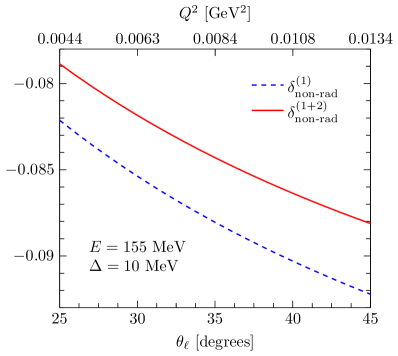
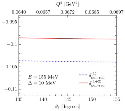
Figure 10: The non-radiative part of the correction factors at first (dashed, blue curve) and second order (full, red curve) in the range of scattering angles relevant for P2: forward scattering with $25^{\circ}<\theta_{\ell}<45^{\circ}$ (left) and backward scattering with $135^{\circ}<\theta_{\ell}<155^{\circ}$ (right). Soft-photon corrections are included with the cut-off fixed at $\Delta=10$ MeV.

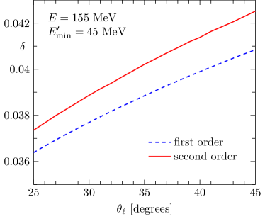
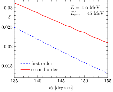
Figure 11: The complete radiative correction factors at first (dashed, blue curve) and second order (full, red curve) in the range of scattering angles relevant for P2: forward scattering with $25^{\circ}<\theta_{\ell}<45^{\circ}$ (left) and backward scattering with $135^{\circ}<\theta_{\ell}<155^{\circ}$ (right). Hard-photon radiation is included with the restriction that the final state electron has an energy above $E^{\prime}_{\rm min}=45$ MeV.

The non-radiative part of the corrections is shown in Fig. 10. In this case, soft-photon radiation is included with the cut-off $\Delta=10$ MeV. The corrections reach the level of some $-8.5\,\%$ and exhibit a moderate $Q^{2}$ dependence. Second-order corrections are small, but are relevant at the level of $0.3$ to $0.5\,\%$. The layout of the P2 spectrometer with a solenoidal magnetic field is constructed in such a way that no bremsstrahlung photon emitted in the target volume can reach the detector. Therefore, radiative scattering will contribute to the measured cross section as long as the scattered electrons fulfil the condition $E^{\prime}>E^{\prime}_{\rm min}$. The complete radiative correction factor including hard-photon radiation is shown in Fig. 11. We find that the cross section is increased significantly by the inclusion of radiative processes. The corrections are now positive, at the level of a few percent. The difference between the first- and second-order calculations turns out to be slightly smaller in the forward region, but can still reach somewhat more than half a percent in the backward region.

While it is not possible at the P2 experiment to impose a veto on hard radiated photons directly, the requirement of a minimum energy $E^{\prime}_{\rm min}$ for the scattered electrons restricts the phase space for photon emission indirectly. This introduces a strong dependence on $E^{\prime}_{\rm min}$. Numerical results are shown in Fig. 12 (left), again both at first and at second order. In the P2 experiment energy loss can also occur when the incoming electron passes through the liquid hydrogen target. It is therefore also important to know how the cross section depends on the energy $E$ of the incoming electrons. Results for the first- and second-order radiative correction factors are shown in the right part of Fig. 12. For reduced $E$ while keeping $E^{\prime}_{\rm min}=45$ MeV fixed, hard-photon radiation will be suppressed and the corrections become negative. The observed strong dependence on $E$ and $E^{\prime}_{\rm min}$ highlights the necessity to include radiative effects in a full Monte-Carlo simulation of the experiment where the acceptance for electron detection may be a complicated function of the scattering angle.

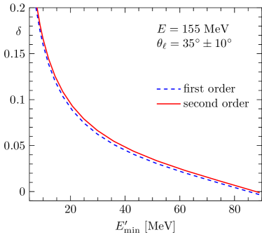
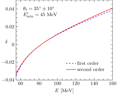
Figure 12: The complete radiative correction factors at first (dashed, blue curve) and second order (full, red curve) for P2 as a function of the cut-off on the energy of the scattered electron $E^{\prime}_{\rm min}$ (left) and as a function of the beam energy with fixed $E^{\prime}_{\rm min}$ (right). The scattering angle was integrated over the range $25^{\circ}\leq\theta_{\ell}\leq 45^{\circ}$.

For a better understanding and for completeness we also show results for the cross section of radiative ep scattering in Fig. 13. This process is, in fact, not measurable at P2. The plot of this figure shows that bremsstrahlung is dominated by far by the emission of photons collinear with the incoming electrons, but there is also a peak in the angular distribution where photons are emitted in the direction of the scattered electron. The one-loop and soft-photon corrections for radiative scattering are negative on the collinear peaks ($-7\,\%$ for $\theta_{\gamma}=\theta_{\ell}=35^{\circ}$) and positive for photon emission angles far away from the peaks ($+11.4\,\%$ for $\theta_{\gamma}\simeq 15^{\circ}$). A particularly interesting feature is a dip on top of the final-state radiation peak, shown in more detail in the upper right corner of Fig. 13. The final-state peak is determined by terms proportional to $1/(l^{\prime}k)$ in the soft-photon eikonal factor, see Eq. (31),

$$\frac{1}{l^{\prime}k}=\frac{1}{E_{\gamma}\left(E^{\prime}-|\vec{l}^{\,\prime}|\cos\psi\right)}\,,$$ (64)

where $\psi$ is the angle between the scattered lepton and the emitted photon. It is obvious that for a photon emitted collinearly with the final-state electron, i.e. for $\psi\rightarrow 0$, and for $m_{\ell}\rightarrow 0$ this term diverges. One can show that for a finite value of the electron mass the dominating terms in the eikonal factor vanish for zero emission angle,

$$\frac{2l^{\prime}l}{(l^{\prime}k)(lk)}-\frac{m_{\ell}^{2}}{(l^{\prime}k)^{2}}\longrightarrow\frac{1}{E_{\gamma}^{2}}\frac{4E^{\prime\,4}}{m_{\ell}^{4}}\psi^{2}$$ (65)

for $\psi\ll m_{\ell}/E^{\prime}\ll 1$, which explains the local minimum in the angular distribution of Fig. 13. The details of this feature depend on the value of the lepton mass and will be particularly important for muon scattering. Effects due to lepton-mass dependent terms in the cross section have been discussed in detail also in Refs. [45, 46]. Our results agree with these references.

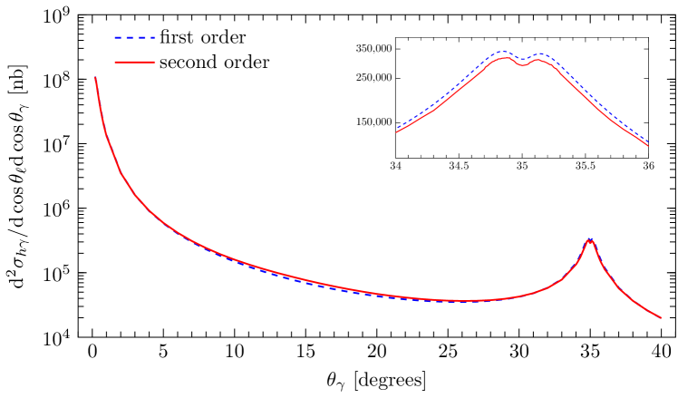
Figure 13: Cross section for radiative scattering with an observed photon of energy $E_{\gamma}\geq\Delta=10$ MeV at tree level (first order, blue dashed line) and including the effect due one-loop corrections and a second unobserved soft photon with energy below the cut-off $\Delta=10$ MeV (second order, full red line). The beam energy is $E=155$ MeV and the scattering angle of the electron fixed at $\theta_{\ell}=35^{\circ}$. The energy of the scattered electron is integrated over the range $E^{\prime}>45$ MeV.

In Figure 14 we show an example of results for the radiative correction factor relevant for the Qweak experiment. Here the beam energy is $E=1.16$ GeV and the experiment covers scattering angles between $5.8^{\circ}$ and $11.6^{\circ}$. The corrections are similar to the case of P2 and reach the level of roughly 5 %. The corrections at second order are smaller than at first order by an order of magnitude.

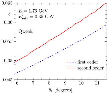
Figure 14: The complete radiative correction factors at first (dashed, blue curve) and second order (full, red curve) in the range of scattering angles relevant for Qweak at $E=1.76$ GeV. Hard-photon radiation is included with the restriction $E^{\prime}_{\rm min}=0.35$ GeV.

Finally we conclude the discussion with a few results for the planned MUSE experiment where also the scattering of muons off protons will be measured. The beam momentum is fixed at $|\vec{l}|=210$ MeV and we do not impose a restriction on the energy of the final-state muon. Results are shown in Fig. 15. The corrections are rather small and vary between $-0.1\,\%$ and $-0.9\,\%$. For the calculation of the second-order corrections in this figure we have used the expression Eq. (46) taken from Ref. [40]. This formula is known to be valid for large momentum transfer and maybe not applicable in the range of scattering angles in the MUSE experiment.

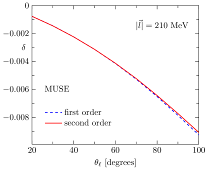
Figure 15: The complete radiative correction factors at first (dashed, blue curve) and second order (full, red curve) in the range of scattering angles relevant for muon scattering at the planned MUSE experiment. Hard-photon radiation is included without an additional restriction, i.e. $E^{\prime}_{\rm min}=m_{\mu}$. The soft-photon cut-off is fixed at $\Delta=0.01$ MeV and we have used Eq. (46) for the 2-loop corrections [40].

As a test we show in Fig. 16 the non-radiative correction factor over a larger range of $Q^{2}$ values and using two alternative expressions taken from Ref. [43]. The one denoted “Mastrolia $Q^{2}\rightarrow\infty$” contains additional lepton mass dependent terms up to and including 4th powers of $\mu=\left(m_{\ell}^{2}/Q^{2}\right)$ and the option denoted “Mastrolia $Q^{2}\rightarrow 0$” includes terms up to $\mu^{-4}$. Our expression derived from Hill’s result, Eq. (46), agrees with Ref. [43] at large $Q^{2}$, as expected, and seems to provide a nice interpolation between the large-$Q^{2}$ and small-$Q^{2}$ limits of Ref. [43], but this may be accidental. For a conclusive interpretation of a high-precision measurement of muon scattering, a calculation of 2-loop and 2-photon corrections taking into account the full mass dependence will be needed. We mention that radiative corrections for the MUSE experiment based on an alternative approach have also been studied recently in Ref. [47].

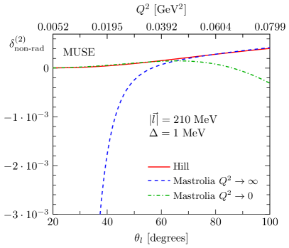
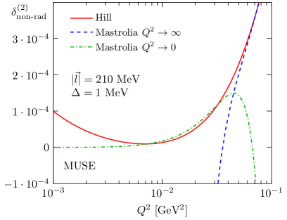
Figure 16: The second-order non-radiative part of the corrections for muon scattering at the MUSE experiment using different approximations from Refs. [43, 40] as described in the text.

7 Concluding remarks

We have calculated leptonic QED corrections for elastic lepton nucleon scattering at first and second order, i.e. including one- and two-loop virtual corrections and one- and two-photon real radiation. Our study of numerical results, in particular for the P2 experiment in Mainz, shows that radiative corrections have to be analysed with care taking into account experimental details which restrict the phase space for photon radiation. Second-order corrections are generally small and will become relevant for measurements at the per mill level. We plan to make the Monte Carlo simulation program, which implements these corrections, publicly available in the near future.

At the time being, our calculation is restricted to the leptonic part of corrections. The inclusion of radiation at the nucleon and two-photon exchange processes will require additional work. In particular, a well-defined separation of corrections contained in the effective nucleon form factors from corrections which can be subtracted during data analysis has still to be worked out. The extension of the calculation for the polarization dependent part, i.e. including Feynman diagrams with $Z$-boson exchange, is in preparation. This calculation will be needed for the planned high-precision measurement of the weak charge of the proton at the P2 experiment.

Appendix A Cross-sections for $ep\rightarrow ep$ and $ep\rightarrow ep\gamma$

The matrix element squared for non-radiative ep scattering, averaged and summed over the spin degrees of freedom in the initial and final states, can be given in a compact form using the following form factor combinations:

$$G\equiv-2Q^{2}\left(F_{1}^{p}+F_{2}^{p}\right)^{2}\,,\quad\quad H\equiv 4\left(F_{1}^{p}\right)^{2}+\frac{Q^{2}}{M^{2}}\left(F_{2}^{p}\right)^{2}\,.$$ (66)

We find

$$\frac{\mathrm{d}\sigma^{(0)}}{\mathrm{d}Q^{2}}=\frac{\overline{|\mathcal{M}_{\text{Born}}|^{2}}}{16\pi\left[(s-m_{\ell}^{2}-M^{2})^{2}-m_{\ell}^{2}M^{2}\right]}$$ (67)

with

$$\overline{\left|\mathcal{M}_{\text{Born}}\right|^{2}}=\frac{(4\pi\alpha)^{2}}{Q^{4}}\left\{G(2m_{e}^{2}-Q^{2})-H\left[M^{2}Q^{2}+\left(s-m_{e}^{2}-M^{2}\right)\left(Q^{2}-s+m_{e}^{2}+M^{2}\right)\right]\right\}\,,$$ (68)

and $s=(l+p)^{2}$. For the matrix element squared of the radiative process with one additional photon, it is convenient to introduce also the variables $S=2l_{1}\cdot p_{1}$ and $U=-2l_{2}\cdot p_{1}$. We find for the matrix element squared for $ep\rightarrow ep\gamma$, averaged and summed over initial and final state spin degrees of freedom:

$$\overline{\left|\mathcal{M}_{1\gamma}\right|^{2}} = \frac{(4\pi\alpha)^{3}}{Q^{4}}\frac{1}{(l_{1}k)^{2}(2l_{1}k+Q^{2}_{\ell}-Q^{2})^{2}}\bigg{\{}$$

$$\quad G\Big{[}-16(l_{1}k)^{4}-16(l_{1}k)^{3}(Q^{2}_{\ell}-Q^{2})+(l_{1}k)^{2}(8m_{\ell}^{2}Q^{2}_{\ell}-6Q^{4}_{\ell}+8Q^{2}_{\ell}Q^{2}-6Q^{4})$$

$$\quad\quad-l_{1}k(Q^{2}_{\ell}-Q^{2})(-4m_{\ell}^{2}Q^{2}_{\ell}+Q^{4}_{\ell}+Q^{4})-m_{\ell}^{2}(2m_{\ell}^{2}-Q^{2})(Q^{2}_{\ell}-Q^{2})^{2}\Big{]}$$

$$\quad-H\Big{[}16(l_{1}k)^{4}M^{2}+8(l_{1}k)^{3}\big{(}2M^{2}(Q^{2}_{\ell}-Q^{2})+\frac{1}{2}Q^{2}(S-U)\big{)}$$

$$\quad\quad+2(l_{1}k)^{2}\left(2m_{\ell}^{2}(Q^{2}-S-U)^{2}+Q^{2}Q^{2}_{\ell}(2S-U)+Q^{4}(S-2U)\right.$$

$$\quad\quad\left.+Q^{2}(S^{2}+U^{2})+M^{2}(3Q^{4}_{\ell}-4Q^{2}_{\ell}Q^{2}+3Q^{4})\right)$$

$$\quad\quad+l_{1}k(Q^{2}_{\ell}-Q^{2})\left(2m_{\ell}^{2}(Q^{2}-2U)(Q^{2}-S-U)\right.$$

$$\quad\quad\left.-Q^{2}(-Q^{2}_{\ell}S-Q^{2}U+S^{2}+U^{2})+M^{2}(Q^{4}_{\ell}+Q^{4})\right)$$

$$\quad\quad-m_{\ell}^{2}(Q^{2}_{\ell}-Q^{2})^{2}\left(M^{2}Q^{2}+U(Q^{2}-U)\right)\Big{]}\bigg{\}}\,.$$

Appendix B Phase-space for one-photon bremsstrahlung, $ep\rightarrow ep\gamma$

After integrating out the final-state nucleon momentum to remove the $\delta$-function for energy-momentum conservation, the phase space for $\ell p\rightarrow\ell p\gamma$ is given by

$$\mathrm{d}^{4}\Gamma=\int\frac{1}{(2\pi)^{5}}\frac{\mathrm{d}^{3}l^{\prime}}{2E^{\prime}}\frac{\mathrm{d}^{3}k}{2E_{\gamma}}\delta\left[(l+p-l^{\prime}-k)^{2}-M^{2}\right]\,.$$ (70)

Using energies and angles as shown in Fig. 1 we write

$$\mathrm{d}^{3}l^{\prime}=E^{\prime}\,|\vec{l}^{\,\prime}|\,\mathrm{d}\cos\theta_{\ell}\,\mathrm{d}\phi_{\ell}\,\mathrm{d}E^{\prime}\,,$$

$$\mathrm{d}^{3}k=E_{\gamma}^{2}\,\mathrm{d}\cos\theta_{\gamma}\,\mathrm{d}\phi_{\gamma}\,\mathrm{d}E_{\gamma}\,,$$

$$(l+p-l^{\prime}-k)^{2}-M^{2}=2(A-B\cos\phi_{\gamma})$$ (71)

with

$$A= M(E-E^{\prime}-E_{\gamma})-EE^{\prime}+E^{\prime}E_{\gamma}-EE_{\gamma}+|\vec{l}||\vec{l}^{\,\prime}|\cos\theta_{\ell}$$

$$+|\vec{l}|E_{\gamma}\cos\theta_{\gamma}-E_{\gamma}|\vec{l}^{\,\prime}|\cos\theta_{\ell}\cos\theta_{\gamma}+m_{\ell}^{2}\,,$$

$$B= E_{\gamma}|\vec{l}^{\,\prime}|\sin\theta_{\ell}\sin\theta_{\gamma}\,.$$ (72)

For unpolarized scattering, one can perform the integration over the azimuthal angle of the scattered lepton $\phi_{\ell}$ and we find

$$\mathrm{d}\Gamma =\int\frac{1}{4(2\pi)^{4}}E_{\gamma}|\vec{l}^{\,\prime}|\,\mathrm{d}E^{\prime}\,\mathrm{d}\cos\theta_{\ell}\,\mathrm{d}E_{\gamma}\,\mathrm{d}\cos\theta_{\gamma}\,\mathrm{d}\phi_{\gamma}\,\delta\left[2(A-B\cos\phi_{\gamma})\right]$$

$$=\frac{1}{8(2\pi)^{4}}\,\frac{\mathrm{d}E^{\prime}\,\mathrm{d}\cos\theta_{\ell}\,\mathrm{d}E_{\gamma}\,\mathrm{d}\cos\theta_{\gamma}}{\sin\theta_{\ell}\sin\theta_{\gamma}\sin\phi_{\gamma}}\,\Theta\left(1-\frac{A^{2}}{B^{2}}\right)\,,$$ (73)

where $\sin\phi_{\gamma}=\sqrt{1-A^{2}/B^{2}}$. Integration limits follow from the condition

$$\frac{A^{2}}{B^{2}}\leq 1\,.$$ (74)

We find

$$m_{\ell}<E^{\prime}<E\,,$$ (75)

$$\max\left(\frac{EE^{\prime}-M(E-E^{\prime})-m_{\ell}^{2}}{|\vec{l}||\vec{l}^{\,\prime}|}\,,-1\right)<\cos\theta_{\ell}<1\,,$$

$$\frac{y}{a-x}<E_{\gamma}<-\frac{y}{a+x}\,,$$

$$\frac{-F\sqrt{F^{2}+D^{2}-C^{2}}-DC}{D^{2}+F^{2}}<\cos\theta_{\gamma}<\frac{F\sqrt{F^{2}+D^{2}-C^{2}}-DC}{D^{2}+F^{2}}\,,$$

where we have used

$$C= M(E-E^{\prime}-E_{\gamma})-EE^{\prime}+E^{\prime}E_{\gamma}-EE_{\gamma}+|\vec{l}||\vec{l}^{\,\prime}|\cos\theta_{\ell}+m_{\ell}^{2}\,,$$

$$D= E_{\gamma}(|\vec{l}|-|\vec{l}^{\,\prime}|\cos\theta_{\ell})\,,$$

$$F= E_{\gamma}|\vec{l}^{\,\prime}|\sin\theta_{\ell}\,,$$

$$a= \sqrt{|\vec{l}|^{2}+|\vec{l}^{\,\prime}|^{2}-2|\vec{l}||\vec{l}^{\,\prime}|\cos\theta_{\ell}}\,,$$

$$x= E^{\prime}-E-M\,,$$

$$y= M(E-E^{\prime})-EE^{\prime}+|\vec{l}||\vec{l}^{\,\prime}|\cos\theta_{\ell}+m_{\ell}^{2}\,.$$

Appendix C Phase-space for two-photon bremsstrahlung, $ep\rightarrow ep\gamma\gamma$

We use the same notation as shown in Fig. 1, but consider two photons in the final state, whose 4-momenta are denoted by $k$ and $k^{\prime}$ with energies $E_{\gamma}$, $E_{\gamma}^{\prime}$ and angles $\theta_{\gamma}$, $\theta_{\gamma}^{\prime}$, $\phi_{\gamma}$, and $\phi_{\gamma}^{\prime}$, respectively. Using the $\delta$ function from energy-momentum conservation, the integration over the 4-particle phase space can be written as

$$\mathrm{d}^{7}\Gamma_{2\gamma}=\frac{E_{\gamma}E^{\prime}_{\gamma}|\vec{l}^{\,\prime}|}{16(2\pi)^{7}}\frac{\mathrm{d}E^{\prime}\,\mathrm{d}\cos\theta_{\ell}\,\mathrm{d}E_{\gamma}\,\mathrm{d}E^{\prime}_{\gamma}\,\mathrm{d}\cos\theta^{\prime}_{\gamma}\,\mathrm{d}\phi^{\prime}_{\gamma}\,\mathrm{d}\cos\theta_{\gamma}}{\left|\alpha_{1}\cos\phi_{\gamma}-\alpha_{2}\sin\phi_{\gamma}\right|}$$ (76)

where

$$\phi_{\gamma}=\arcsin\frac{\alpha_{3}}{\sqrt{\alpha^{2}_{1}+\alpha^{2}_{2}}}-\arcsin\frac{\alpha_{2}}{\sqrt{\alpha^{2}_{1}+\alpha^{2}_{2}}}$$ (77)

with

$$\alpha_{1}= E_{\gamma}E^{\prime}_{\gamma}\sin\theta_{\gamma}\sin\theta^{\prime}_{\gamma}\sin\phi^{\prime}_{\gamma}\,,$$

$$\alpha_{2}= |\vec{l}^{\,\prime}|E_{\gamma}\sin\theta_{\ell}\sin\theta_{\gamma}+E_{\gamma}E^{\prime}_{\gamma}\sin\theta_{\gamma}\sin\theta^{\prime}_{\gamma}\cos\phi^{\prime}_{\gamma}\,,$$

$$\alpha_{3}= m_{\ell}^{2}+M(E-E^{\prime}-E_{\gamma}-E^{\prime}_{\gamma})-E(E^{\prime}+E_{\gamma}+E^{\prime}_{\gamma})+E^{\prime}(E_{\gamma}+E^{\prime}_{\gamma})+|\vec{l}||\vec{l}^{\,\prime}|\cos\theta_{\ell}$$

$$+|\vec{l}|E_{\gamma}\cos\theta_{\gamma}+|\vec{l}|E^{\prime}_{\gamma}\cos\theta^{\prime}_{\gamma}-|\vec{l}^{\,\prime}|E^{\prime}_{\gamma}(\sin\theta_{\ell}\sin\theta^{\prime}_{\gamma}\cos\phi^{\prime}_{\gamma}+\cos\theta_{\ell}\cos\theta^{\prime}_{\gamma})$$

$$-|\vec{l}^{\,\prime}|E_{\gamma}\cos\theta_{\ell}\cos\theta_{\gamma}-E_{\gamma}E^{\prime}_{\gamma}\cos\theta_{\gamma}\cos\theta^{\prime}_{\gamma}+E_{\gamma}E^{\prime}_{\gamma}\,.$$

Integration limits for angles and energies follow from the condition that the arguments of the $\arcsin$-functions in the expression for $\phi_{\gamma}$ in Eq. (77) have to be in the allowed range between $-1$ and $+1$. The required calculations are straightforward, but tedious, and we write down only a few partial results in the following. For $\theta_{\gamma}$ we find:

$$\frac{-\beta_{2}\beta_{3}-\beta_{1}\sqrt{\beta}}{\beta_{1}^{2}+\beta_{2}^{2}}<\cos\theta_{\gamma}<\frac{-\beta_{2}\beta_{3}+\beta_{1}\sqrt{\beta}}{\beta_{1}^{2}+\beta_{2}^{2}}$$ (78)

with

$$\beta_{1}= \sqrt{2E_{\gamma}^{2}|\vec{l}^{\,\prime}|E^{\prime}_{\gamma}\sin\theta_{\ell}\sin\theta^{\prime}_{\gamma}\cos\phi^{\prime}_{\gamma}+E_{\gamma}^{2}E_{\gamma}^{\prime\,2}\sin^{2}\theta^{\prime}_{\gamma}+|\vec{l}^{\,\prime}|^{2}E_{\gamma}^{2}\sin^{2}\theta_{\ell}}\,,$$

$$\beta_{2}= |\vec{l}|E_{\gamma}-|\vec{l}^{\,\prime}|E_{\gamma}\cos\theta_{\ell}-E_{\gamma}E^{\prime}_{\gamma}\cos\theta^{\prime}_{\gamma}\,,$$

$$\beta_{3}= m_{\ell}^{2}+M(E-E^{\prime}-E_{\gamma}-E^{\prime}_{\gamma})-E(E^{\prime}+E_{\gamma}+E^{\prime}_{\gamma})+E^{\prime}(E_{\gamma}+E^{\prime}_{\gamma})+|\vec{l}||\vec{l}^{\,\prime}|\cos\theta_{\ell}$$

$$+|\vec{l}|E^{\prime}_{\gamma}\cos\theta^{\prime}_{\gamma}-|\vec{l}^{\,\prime}|E^{\prime}_{\gamma}(\sin\theta_{\ell}\sin\theta^{\prime}_{\gamma}\cos\phi^{\prime}_{\gamma}+\cos\theta_{\ell}\cos\theta^{\prime}_{\gamma})+E_{\gamma}E^{\prime}_{\gamma}\,.$$

The integration limits for $\phi^{\prime}_{\gamma}$ are:

$$\frac{E_{\gamma}^{2}+\gamma_{2}-E_{\gamma}\sqrt{\gamma}}{\gamma_{1}}<\cos\phi^{\prime}_{\gamma}<\frac{E_{\gamma}^{2}+\gamma_{2}+E_{\gamma}\sqrt{\gamma}}{\gamma_{1}}$$ (79)

with

$$\gamma=2\gamma_{2}+\gamma_{3}>0$$ (80)

and

$$\gamma_{1}= |\vec{l}^{\,\prime}|E^{\prime}_{\gamma}\sin\theta_{\ell}\sin\theta^{\prime}_{\gamma}\,,$$ (81)

$$\gamma_{2}= m_{\ell}^{2}+M(E-E^{\prime}-E_{\gamma}-E^{\prime}_{\gamma})-E(E^{\prime}+E_{\gamma}+E^{\prime}_{\gamma})+E^{\prime}(E_{\gamma}+E^{\prime}_{\gamma})$$ (82)

$$+E_{\gamma}E^{\prime}_{\gamma}+|\vec{l}||\vec{l}^{\,\prime}|\cos\theta_{\ell}+E^{\prime}_{\gamma}\cos\theta^{\prime}_{\gamma}\left(|\vec{l}|-|\vec{l}^{\,\prime}|\cos\theta_{\ell}\right)\,,$$

$$\gamma_{3}= |\vec{l}|^{2}+|\vec{l}^{\,\prime}|^{2}+E_{\gamma}^{2}+E_{\gamma}^{\prime\,2}-2E^{\prime}_{\gamma}\cos\theta^{\prime}_{\gamma}\left(|\vec{l}|-|\vec{l}^{\,\prime}|\cos\theta_{\ell}\right)-2|\vec{l}||\vec{l}^{\,\prime}|\cos\theta_{\ell}\,.$$ (83)

The condition $\gamma\geq 0$ is always fulfilled provided that

$$E^{\prime}_{\gamma}\leq E-E^{\prime}-E_{\gamma}\,.$$ (84)

In our implementation of the numerical integration over the phase space we make sure that no kinematic limit is missed by reconstructing always complete events and checking the 4-momentum conservation. This allows us to use the phase space integrator as an event generator which can be used for the simulation of an experiment. It turns out that an explicit implementation of the kinematic limits given above in the numerical integration routine is sufficient to render the efficiency of the Monte Carlo integration at a high level above $70\,\%$.

References

- [1] D. Androić et al. [Qweak Collaboration], Nature 557 (2018) 207.
- [2] D. Becker et al., arXiv:1802.04759 [nucl-ex].
- [3] R. Gilman et al. [MUSE Collaboration], arXiv:1303.2160 [nucl-ex].
- [4] L. W. Mo and Y. S. Tsai, Rev. Mod. Phys. 41 (1969) 205.
- [5] Y. S. Tsai, Phys. Rev. 122 (1961) 1898.
- [6] Y. S. Tsai, SLAC-PUB-0848.
- [7] C. de Calan, H. Navelet and J. Picard, Nucl. Phys. B 348 (1991) 47.
- [8] L. C. Maximon and J. A. Tjon, Phys. Rev. C 62 (2000) 054320 [nucl-th/0002058].
- [9] F. Weissbach, K. Hencken, D. Rohe, I. Sick and D. Trautmann, Eur. Phys. J. A 30 (2006) 477 [nucl-th/0411033].
- [10] F. Weissbach, K. Hencken, D. Rohe and D. Trautmann, Phys. Rev. C 80 (2009) 024602 [arXiv:0805.1535 [nucl-th]].
- [11] I. Akushevich, H. Gao, A. Ilyichev and M. Meziane, Eur. Phys. J. A 51 (2015) 1.
- [12] I. Akushevich and A. Ilyichev, Phys. Rev. D 85 (2012) 053008 [arXiv:1201.4065 [hep-ph]].
- [13] I. Akushevich and A. Ilyichev, arXiv:1712.00091 [hep-ph].
- [14] A. B. Arbuzov and T. V. Kopylova, Eur. Phys. J. C 75 (2015) 603 [arXiv:1510.06497 [hep-ph]].
- [15] E. A. Kuraev, A. I. Ahmadov, Y. M. Bystritskiy and E. Tomasi-Gustafsson, Phys. Rev. C 89 (2014) 065207 [arXiv:1311.0370 [hep-ph]].
- [16] D. Borisyuk and A. Kobushkin, Phys. Rev. C 90 (2014) 025209 [arXiv:1405.2467 [hep-ph]].
- [17] R. E. Gerasimov and V. S. Fadin, J. Phys. G 43 (2016) 125003 [arXiv:1604.07960 [nucl-th]].
- [18] J. Arrington, P. G. Blunden and W. Melnitchouk, Prog. Part. Nucl. Phys. 66 (2011) 782 [arXiv:1105.0951 [nucl-th]].
- [19] R. Ent, B. W. Filippone, N. C. R. Makins, R. G. Milner, T. G. O’Neill and D. A. Wasson, Phys. Rev. C 64 (2001) 054610.
- [20] G. I. Gakh, M. I. Konchatnij, N. P. Merenkov and E. Tomasi-Gustafsson, Phys. Rev. C 95 (2017) 055207 [arXiv:1612.02139 [hep-ph]].
- [21] A. Kwiatkowski, H. Spiesberger and H. J. Möhring, Comput. Phys. Commun. 69 (1992) 155.
- [22] A. Arbuzov, D. Y. Bardin, J. Blümlein, L. Kalinovskaya and T. Riemann, Comput. Phys. Commun. 94 (1996) 128 [hep-ph/9511434].
- [23] A. V. Afanasev, I. Akushevich, A. Ilyichev and N. P. Merenkov, Phys. Lett. B 514 (2001) 269 [hep-ph/0105328].
- [24] K. Charchula, G. A. Schuler and H. Spiesberger, Comput. Phys. Commun. 81 (1994) 381.
- [25] I. Akushevich, O. F. Filoti, A. N. Ilyichev and N. Shumeiko, Comput. Phys. Commun. 183 (2012) 1448 [arXiv:1104.0039 [hep-ph]].
- [26] R. D. Bucoveanu and H. Spiesberger, in preparation.
- [27] S. D. Drell and J. D. Walecka, Annals Phys. 28 (1964) 18.
- [28] V. Shtabovenko, R. Mertig and F. Orellana, Comput. Phys. Commun. 207 (2016) 432 [arXiv:1601.01167 [hep-ph]].
- [29] T. Hahn and M. Perez-Victoria, Comput. Phys. Commun. 118 (1999) 153 [hep-ph/9807565].
- [30] M. Vanderhaeghen, J. M. Friedrich, D. Lhuillier, D. Marchand, L. Van Hoorebeke and J. Van de Wiele, Phys. Rev. C 62 (2000) 025501 [hep-ph/0001100].
- [31] V. V. Bytev, E. A. Kuraev and E. Tomasi-Gustafsson, Phys. Rev. C 77 (2008) 055205 [hep-ph/0310226].
- [32] G. ’t Hooft and M. J. G. Veltman, Nucl. Phys. B 153 (1979) 365.
- [33] A. V. Gramolin, V. S. Fadin, A. L. Feldman, R. E. Gerasimov, D. M. Nikolenko, I. A. Rachek and D. K. Toporkov, J. Phys. G 41 (2014) 115001 [arXiv:1401.2959 [nucl-ex]].
- [34] T. Hahn, Comput. Phys. Commun. 168 (2005) 78 [hep-ph/0404043].
- [35] A. O. G. Kallen and A. Sabry, Kong. Dan. Vid. Sel. Mat. Fys. Med. 29 (1955) 17, 1.
- [36] F. Ignatov, http://cmd.inp.nsk.su/~ignatov/vpl/
- [37] S. Actis et al. [Working Group on Radiative Corrections and Monte Carlo Generators for Low Energies], Eur. Phys. J. C 66 (2010) 585 [arXiv:0912.0749 [hep-ph]].
- [38] F. Jegerlehner, Nuovo Cim. C 034S1 (2011) 31 [arXiv:1107.4683 [hep-ph]].
- [39] A. Keshavarzi, D. Nomura and T. Teubner, Phys. Rev. D 97 (2018) no.11, 114025 [arXiv:1802.02995 [hep-ph]].
- [40] R. J. Hill, Phys. Rev. D 95 (2017) 013001 [arXiv:1605.02613 [hep-ph]].
- [41] T. van Ritbergen and R. G. Stuart, Phys. Lett. B 437 (1998) 201 [hep-ph/9802341].
- [42] A. I. Davydychev, K. Schilcher and H. Spiesberger, Eur. Phys. J. C 19 (2001) 99 [hep-ph/0011221].
- [43] P. Mastrolia and E. Remiddi, Nucl. Phys. B 664 (2003) 341 [hep-ph/0302162].
- [44] R. Bonciani, P. Mastrolia and E. Remiddi, Nucl. Phys. B 676 (2004) 399 [hep-ph/0307295].
- [45] M. B. Barbaro, C. Maieron and E. Voutier, Phys. Lett. B 726 (2013) 505, Erratum: [Phys. Lett. B 727 (2013) 573] [arXiv:1305.3873 [hep-ph]].
- [46] P. Talukdar, F. Myhrer and U. Raha, arXiv:1712.09963 [nucl-th].
- [47] P. Talukdar, F. Myhrer, G. Meher and U. Raha, arXiv:1810.04027 [nucl-th].