The Cross-correlation of KSZ Effect and 21 cm Intensity Mapping with Tidal Reconstruction

Abstract

We discuss the possibility of studying diffuse baryon distributions with kinematic Sunyaev-Zel’dovich (kSZ) effect by correlating cosmic microwave background (CMB) temperature fluctuations with density fluctuations from 21 cm intensity mapping (IM). The biggest challenge for the cross-correlation is the loss of large-scale information in IM, due to foregrounds and the zero spacing problem of interferometers. We apply the tidal reconstruction algorithm to restore the lost large-scale modes, which increases the correlation by more than a factor of three. With the predicted foreground level, we expect a $\sim 20\,\sigma$ detection of kSZ signal for $0.8\lesssim z\lesssim 2.5$ with CHIME and Planck, and a $\sim 40\,\sigma$ detection with HIRAX and Planck. The significance can be greatly increased with next-generation facilities of higher spatial resolutions.

I Introduction

For $z\lesssim 2$, a large fraction of the predicted baryon content is missing in observations. The majority of these baryons are believed to reside in the warm-hot intergalactic medium (WHIM), with typical temperatures of $10^{5}$ K to $10^{7}$ K Davé et al. (2001); Pen (1999); Sołtan (2006). The low density imposes difficulties for direct detection. The uncertainty in the spatial distribution of its ionization state, metallicity, and pressure leads to confusion in interpreting signals from absorption lines and soft X-rays.

The kinematic Sunyaev-Zel’dovich (kSZ) effect Sunyaev and Zeldovich (1972, 1980); Vishniac (1987) is a promising probe for diffuse baryon content. KSZ signal is a secondary anisotropy in cosmic microwave background (CMB) temperature, which comes from the Doppler shift of photons induced by the radial velocity of free electrons. It has the following advantages: First of all, it receives a contribution from all the free electrons, which traces $\gtrsim 90\%$ Fukugita and Peebles (2004) the baryons at low redshifts. Second, the signal is mainly influenced by the electron density and the radial velocity, regardless of the temperature, pressure, and metallicity. Therefore, no extra assumptions are required to estimate the baryon abundance. Lastly, the radial velocity is a large-scale field, so the signal is less biased by the local environment, and more indicative of the diffuse distribution. Hence, the kSZ is an unbiased probe for density fluctuations and its strength at different angular scales can be model-independently translated into baryon contents and diffuseness.

Studying the kSZ effect is challenging as its relatively weak compared to the various contaminations, such as the primary CMB, thermal SZ effects, CMB lensing, and instrumentation noises. Another consideration is kSZ is a projected signal with contributions from different redshift mixed together. One way to mitigate the problem is, to cross-correlate CMB map with the density fluctuations from another tracer at a specific redshift. Several types of surveys have been proposed to play the role Hand et al. (2012); Shao et al. (2011); Li et al. (2014); Hill et al. (2016); Ferraro et al. (2016). Galaxy spectroscopic surveys, with accurate redshift information and high angular resolution, are powerful probes of density fluctuations at low redshift for high angular scales, i.e. $\ell>4000$ Schaan et al. (2016). However, the survey speed and cost limit their sky coverage and depth. Especially for $z\sim 1.4-2.5$, lack of spectral lines will lead to large shot noise in the measured density field. Projected field surveys, such as galaxy photometric surveys and gravitational lensing maps, on the other hand, can provide a densely sampled sky up to the high redshift. However, a significant fraction of kSZ signals come from the density fluctuations along the line of sight (LOS) due to the coupling of two fields (see section IV). Cross-correlating it with a survey without LOS structure will inevitably lead to suboptimal correlation and loss of information.

In this paper, we discuss the possibility of cross-correlating neutral hydrogen (HI) density field from 21 cm intensity mapping (IM) experiments with the kSZ signal. 21 cm spectral lines provide accurate redshift information, and IM experiments perform fast scans of large sky area by integrating all photons detected. In the following few years, there will be several large sky IM surveys producing data up to redshift 2.5 Bandura et al. (2014); Xu et al. (2015); Newburgh et al. (2016). The foreground contaminations, zero-spacing of interferometers and small scale noises of IM are main factors that will downgrade the correlation. The loss of large-scale information makes it almost impossible to cross correlate the IM surveys with other projected field surveys. After estimating the influence of these aspects for the correlation with kSZ effect, we demonstrate how the tidal reconstruction algorithmPen et al. (2012); Zhu et al. (2016a, b); Foreman et al. (2018) can increase the correlation.

The paper is organized as follows: Section II describes how to cross-correlate density fields with CMB temperature fluctuations (following Ref. Shao et al. (2011)); Section III addresses the limits of 21cm IM surveys and its influence on the correlations; Section IV demonstrates the scales of density and velocity fluctuations that contributes most in kSZ distortions; Section V summarizes the tidal reconstruction algorithm which reconstructs the missing large-scale modes; Section VI presents numerical results and expected S/N; We conclude in Sec. VII.

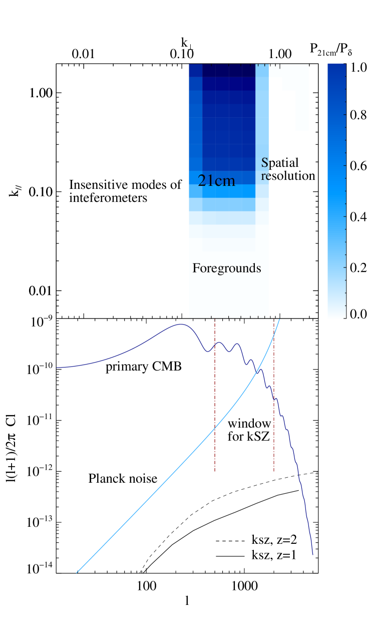
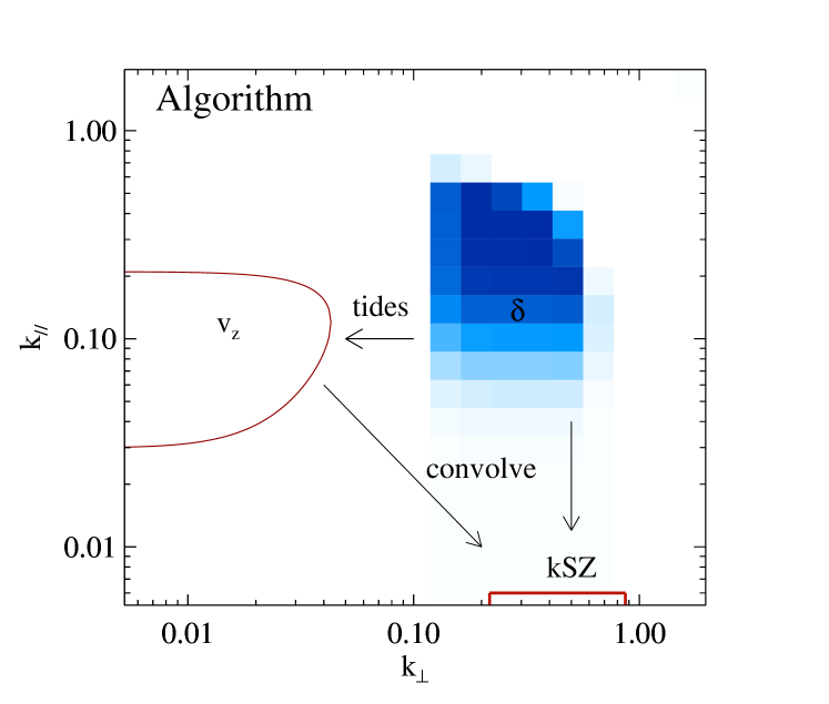
Figure 1: (Top) The detectable scales of density fluctuations in 21 cm intensity mapping experiments with CHIME at redshift 1. (Middle) The angular power spectrum of kSZ signals from two boxes of conformal distance 1 Gpc/$h$ centered at redshift 1 and 2 respectively, as opposed to those of primary CMB and of instrument noises from Planck at 217 GHz. (Bottom) The generation of kSZ signals convolves density and velocity field of different spatial scales. We use tidal reconstruction algorithm to restore the contaminated large scale modes in intensity mapping. The kSZ template is generated by convolving $v_{z}$ calculated from tidal reconstructed field and $\delta$ from 21 cm intensity mapping.

II Cross-correlation of density fields with kSZ

The CMB temperature fluctuation caused by the kSZ effect is approximately a line-of-sight integral of the free electron momentum field:

$$\Theta_{\mathrm{kSZ}}(\bm{\theta})\equiv\frac{\Delta T_{\mathrm{kSZ}}}{T_{\mathrm{CMB}}}=-\frac{1}{c}\int d\chi g(\chi)p_{\parallel}(\chi,\bm{\theta})\ ,$$ (1)

where $\chi(z)$ is the comoving distance, $g(\chi)=e^{-\tau}d\tau/d\eta$ is the visibility function, $\tau$ is the optical depth of Thomson scattering, $p_{\parallel}=(1+\delta_{e})v_{\parallel}$ is the free electron momentum field parallel to the line of sight, and $\delta_{e}=(\rho-\bar{\rho})/\bar{\rho}$ is the free electron overdensity, with $\bar{\rho}$ denoting the average density. It is assumed that electron overdensity $\delta_{e}$ is closely related to the baryon overdensity at $z<2$, therefore, we simply use $\delta$ to denote both hereafters.

The direct correlation between kSZ and density fields vanishes due to the cancellation of positive and negative velocities, therefore, we follow the kSZ template method Shao et al. (2011) to select for kSZ signals.

The peculiar velocity in a radial direction could be calculated from the linearized continuity equation:

$$v_{z}(\bm{k})=iaHf\delta(\bm{k})\frac{k_{z}}{k^{2}}\,$$ (2)

where $a$ is the scale factor, $f=d\ln D/d\ln a$, $D(a)$ is the linear growth function, $H$ is the Hubble parameter, the indice ‘$z$’ indicates the direction along LOS.

We generate the kSZ template of a selected redshift bin with the measured density field $\delta$ and the calculated radial velocity field $v_{z}$, following Eq (1). Correlating the kSZ template with the CMB distortion selects out the kSZ signal.

To quantify the tightness of correlation between the kSZ template and actual kSZ, we introduce a correlation coefficient $r_{\ell}$:

$$r_{\ell}\equiv\frac{C_{\ell\,\mathrm{tmpl,real}}}{\sqrt{C_{\ell\,\mathrm{tmpl}}C_{\ell\,\mathrm{real}}}}\,$$ (3)

where $C_{\ell\,\mathrm{tmpl,real}}$ is the cross angular power spectrum.

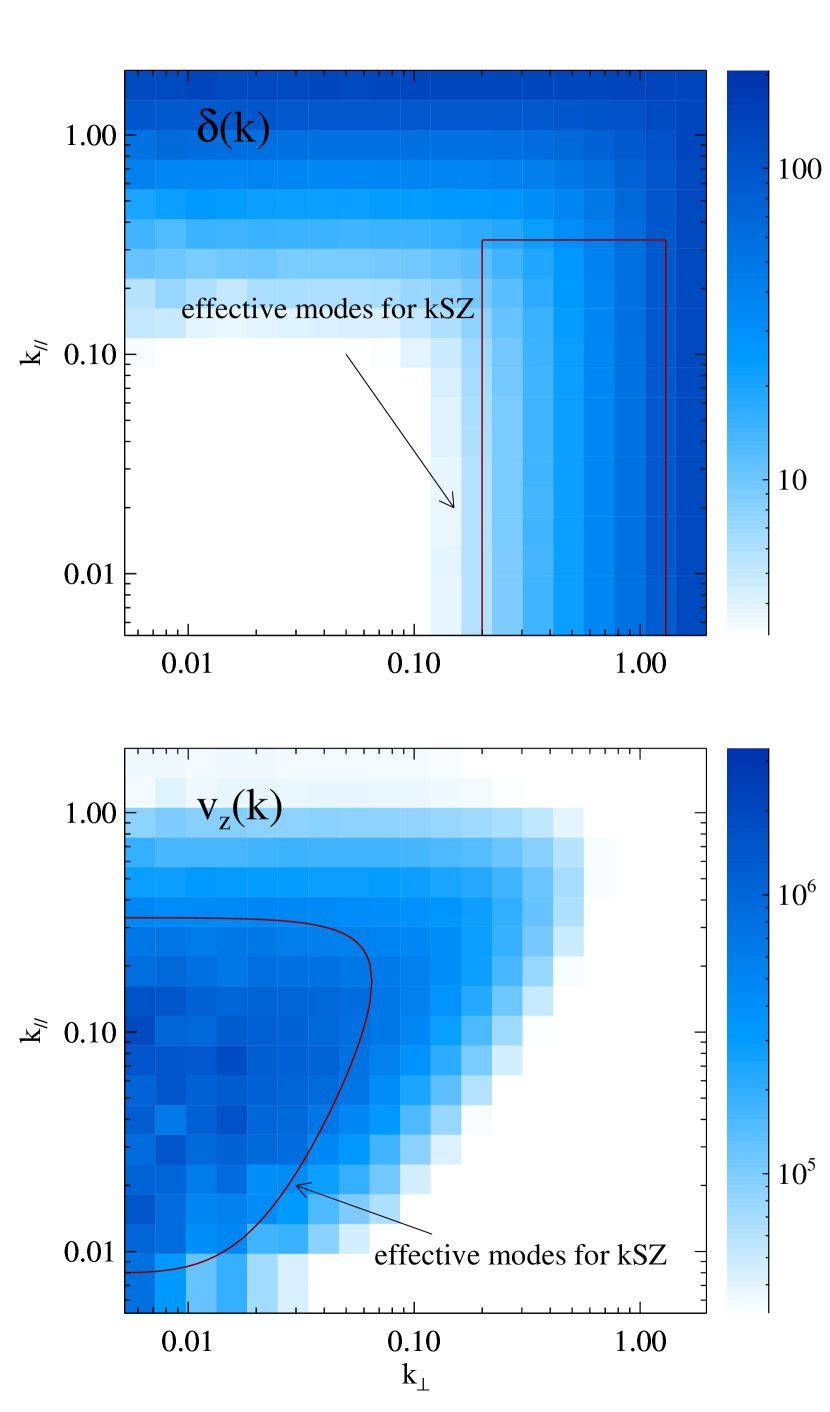
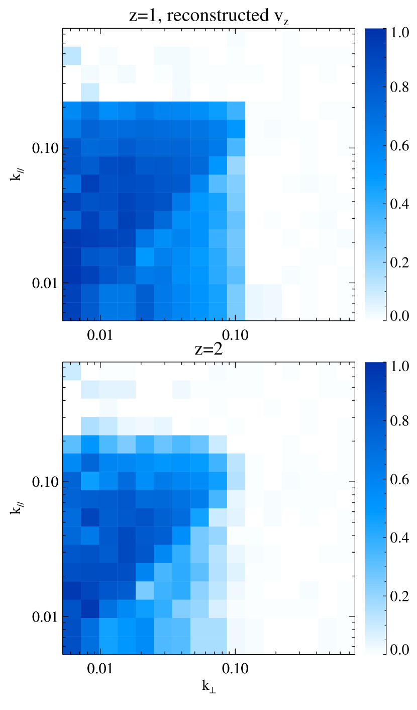
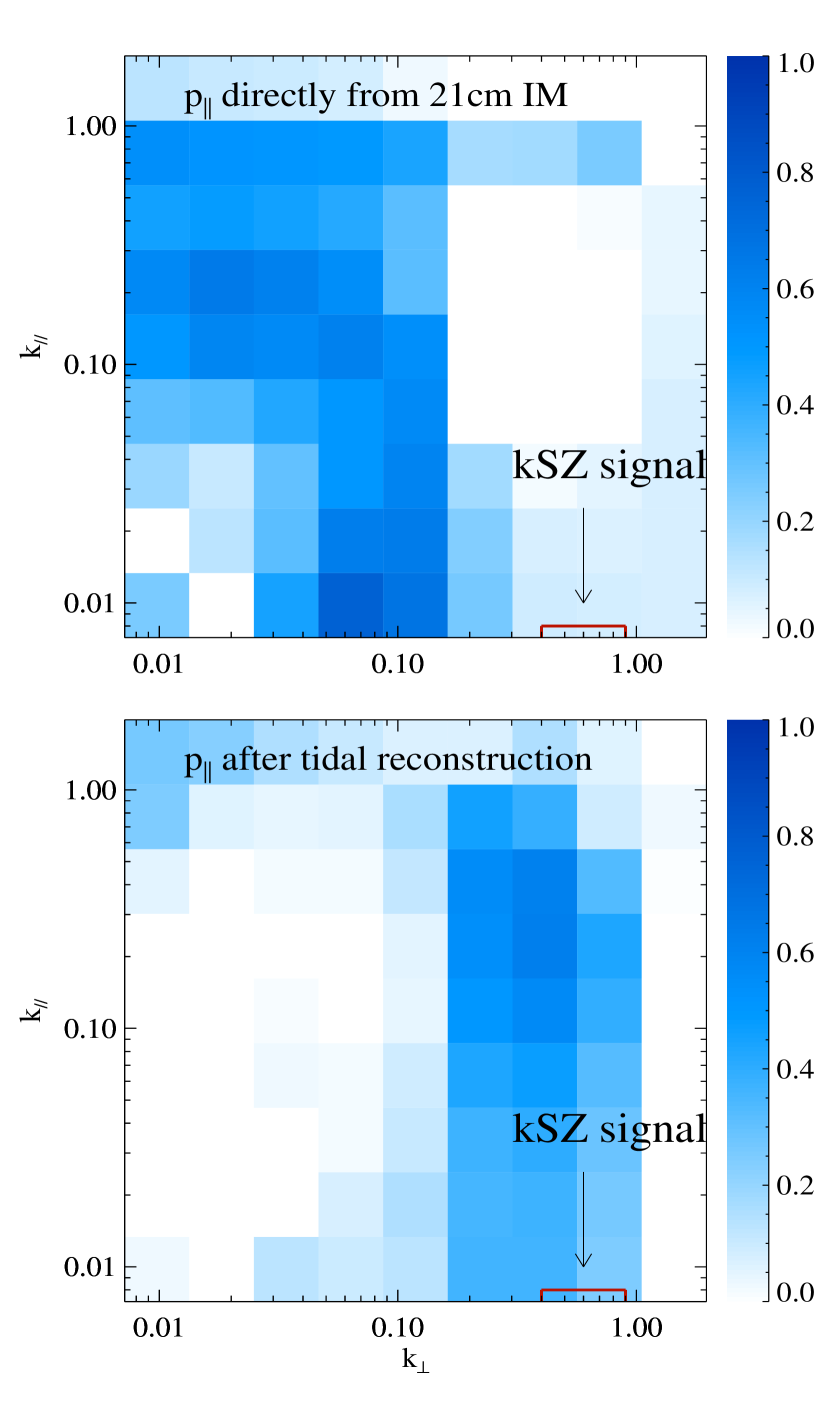
Figure 2: (Left) The color represents the variances $2\pi^{2}\Delta^{2}\equiv k^{3}P(k)$ of the complete density and velocity field at $z=1$. It indicates the weights of different Fourier modes contributing to fields in real space. The modes that are essential for kSZ distortions at $\ell\sim 500-2000$ are marked out. (Middle) The correlation coefficient between the tidal reconstructed $v_{z}$ and actual $v_{z}$ at $z=1~{}\&~{}2$, assuming the original field is collected by CHIME with high foregrounds. (Right) Upper panel shows the correlation coefficient between momentum fields $p_{\parallel}=(1+\delta)v_{z}$ calculated from IM fields and the actual one. Lower panel shows the increased correlation after tidal reconstruction. KSZ signal corresponds to $k_{z}\sim 0$ modes, for which $\ell\sim 500-2000$ is marked out.

III Challenges for 21 cm intensity mapping

Given complete detection of density fluctuations, following the procedures described in the previous section, we should be able to retrieve $>90\%$ of the kSZ signal from CMB at selected redshift bins Shao et al. (2011). However, 21 cm IM experiments are only sensitive to density fluctuations on certain scales, because of the several sources of noises:

1. Foreground noises: IM intends to use all photons to map the density field. While gaining unprecedented survey speed, it leads to severe foreground contamination. The foregrounds, typically three orders of magnitude stronger than the signals, have complicated origins, ranging from galactic emission, extragalactic radio sources, radio recombination lines to the noises from the telescopes Di Matteo et al. (2004); Masui et al. (2013). It will contaminate the signals of large-scale structures in the radial direction.

2. Zero spacing problem of interferometers: Current 21cm IM experiments are all carried on interferometers — on the one hand, they are stable; on the other hand, the cross correlations from different dishes have orders of lower noises than auto-correlations from a single dish. For CHIME-like facilities, with multiple beams installed on one dish, the calibration for cross correlation between two beams of the same dish are complicated. Therefore, we only consider signals from cross correlating different dishes for the rest of the paper. The minimum spacing between dishes, i.e. the shortest baseline of the interferometer, decides the largest angular scale it could probe. It results in an inner hole of small $k_{\perp}$ of sampled density field in the Fourier space.

3. Small scale noises: The smallest scale density fluctuations detectable in 21cm IM experiments are jointly decided by the angular resolution of the facility, i.e. the longest baseline, receiver noise and shot noise. For redshift one, the receiver noise dominates. It gives an upper limit of the Fourier modes we could detect.

Fig. 1 upper panel is an illustration of these effects in density field obtained with 21cm IM. Directly using it to correlate with CMB map from Planck will only retrieve $\sim 10\%$ of the underlying kSZ signal.

IV Important scales for kSZ

In this section, we discuss how different Fourier modes of density and velocity field contribute to the kSZ distortions.

As demonstrated in Fig. 1, the kSZ effect is too faint to be distinguished until the primary CMB starts to fade away, at roughly $\ell>500$. It is possible to select a frequency band where the thermal SZ signal is negligible, then the dominant factor at high $\ell$ will be the CMB instrumental noise. With existing Planck Planck Collaboration et al. (2016) data at 217 GHz, $\ell\sim 500-2000$ will be the visible window for kSZ signal. The window could be extended to higher multipole with Simons Observatory The Simons Observatory Collaboration et al. (2018) and CMB-S4 Abazajian et al. (2016), but for this paper, we focus on $\ell\sim 500-2000$.

Write the kSZ distortion $\Theta(\bm{\theta})$ from a specific redshift in Fourier space as

$$\Theta(\bm{\ell}) \propto p_{\parallel}(\bm{\ell},0)$$ (4)

$$\propto\int d^{3}k\,\delta(\bm{\ell}/\chi(z)-\bm{k}_{\perp},-k_{\parallel})v_{z}(\bm{k_{\perp}},k_{\parallel}).$$

where $\chi(z)$ denotes the comoving distance a redshift $z$, we use it to transform angular scale $\bm{\ell}$ and $\bm{k}_{\perp}$. Notice that $g(\chi)$ is a slow varying function, so it is treated as a constant in this analysis for convenience.

The convolution shows that kSZ combines density and velocity field with different angular scales and identical parallel scales, i.e. not $v_{z}(\bm{k})$ and $\delta(\bm{k})$ with identical $\bm{k}$, but those with $k_{z}$ of same magnitude but a seperation of $\delta\bm{k_{\perp}}=\ell/\chi$ being coupled together. Therefore, the effective modes for $v_{z}$ and $\delta$ come as a pair with $\bm{\ell}/\chi$ separation in Fourier space. A demonstration of this convolution for kSZ $\ell\sim 500-2000$ is indicated in Fig. 1.

Although the summation is over all pairs of $\delta$ and $v_{z}$ with a specific separation in Fourier space, the weight of each pair can be off by orders of magnitude depending on the power spectrum of $\delta$ and $v_{z}$. In Fig. 2 left panels show the variances $2\pi^{2}\Delta^{2}\equiv k^{3}P(k)$ of density and velocity fields at redshift 1. Variance is an effective way to show contribution of different scales — the power spectrum $P(k)$ indicates the strength of $|\delta|$ or $|v_{z}|$ at scale $k$, and $k^{3}$ accounts for the integral in Eq. 4, which is a simple estimator for the space between $k$ and $k+\Delta k$ in log-log plots. Combining the two plots in left panels of Fig. 2, we show that:

1. Within the range of $0.005\lesssim k\lesssim 2$ $h$/Mpc, velocity variance $2\pi^{2}\Delta_{v_{z}}^{2}$ is a small $k_{\perp}$ dominated field while for density variance $2\pi^{2}\Delta_{\delta}^{2}$, large $k_{\perp}$ modes play an important role. Therefore, all the large $\ell$ modes of kSZ comes from coupling of $\delta(\,\mathrm{large}\,k_{\perp})$ with $v_{z}(\,\mathrm{small}\,k_{\perp})$. In other words, almost same large scale modes of $v_{z}$ contribute to all $\ell$s of kSZ, different $\ell$ of kSZ tracks $\delta$ of different spatial scales;

2. In the parallel direction, $k^{3}$ greatly down-weights the large scale $P_{v_{z}}$, leading to middle scale $k_{\parallel}$ modes contributing to $2\pi^{2}\Delta_{v_{z}}^{2}$. Therefore, kSZ signal is not solely from large scale structures along line of sight— a significant fraction of middle scale fluctuations up to few Mpc/h enters the signal from the convolution.

We mark the most relevant modes for generating kSZ signal of $\ell\sim 500-2000$ with red lines in Fig.2. (Notice that although these modes contribute to $\sim 90\%$ of the kSZ signals, but modes with smaller contribution can still be detectable given enough S/N, i.e. at larger $\ell$s when primary CMB fades away, it is possible to probe into even smaller scales. However, this is beyond our discussion here.)

The essential modes for density and velocity field require completely different spacial resolutions. Since the velocity field is linearly constructed from density field, an optimal survey should include essential modes of both fields. Comparing these essential modes with the modes resolvable in 21cm IM (shown in Fig. 2 left panels and Fig.1 upper panel respectively), we notice that while the effective modes for $\delta$ are partly resolved, the large scale dominated $v_{z}$ is almost completely lost in the 21 cm IM. We attempt to recover these modes with cosmic tidal reconstruction Zhu et al. (2016a); Pen et al. (2012).

V Cosmic tidal reconstruction

The density fluctuations on different scales interact under the gravitational interactions during nonlinear structure formation. The evolution of small-scale density fluctuations is modulated by the long wavelength density perturbations Zhu et al. (2016a); Schmidt et al. (2014). By studying the anisotropic tidal distortions of the local small-scale power spectrum, it is possible to solve the tidal field and hence the underlying large-scale structures Pen et al. (2012); Zhu et al. (2016a, b); Foreman et al. (2018).

The leading order effect of the long wavelength perturbation is described by the large-scale tidal field,

$$t_{ij}=\partial_{i}\partial_{j}\Phi_{L}-\nabla^{2}\Phi_{L}\delta_{ij}/3,$$ (5)

where $\delta_{ij}$ is the Kronecker delta function, $\Phi_{L}$ is the long wavelength gravitational potential. Here we focus on the traceless tidal field since the anisotropic distortions are more robust than the change of local power spectrum amplitude which may arise due to other processes. From Lagrangian perturbation theory, the local anisotropic matter power spectrum due to the tidal effect from large-scale density perturbation is

$$P(\bm{k},\tau)|_{t_{ij}}=P(k,\tau)+\hat{k}^{i}\hat{k}^{j}t^{(0)}_{ij}P(k,\tau)f(k,\tau),$$ (6)

where $\hat{k}^{i}$ is the unit vector, $P(k,\tau)$ is the isotropic linear power spectrum, the superscript $(0)$ denotes the initial time defined in perturbation calculation, and $f(k,\tau)$ is the tidal coupling function Zhu et al. (2016a).

The tidal force tensor $t_{ij}$ is symmetric and traceless and hence can be decomposed into five independent observables:

$$t_{ij}=\left(\begin{array}[]{ccc}\gamma_{1}-\gamma_{z}&\gamma_{2}&\gamma_{x}\\ \gamma_{2}&-\gamma_{1}-\gamma_{z}&\gamma_{y}\\ \gamma_{x}&\gamma_{y}&2\gamma_{z}\end{array}\right).$$ (10)

Therefore, from the angular dependence of the tidal shear distortions, we can solve for different components of $t_{ij}$. The reconstruction of gravitational tidal shear fields is described by the same formulation as the weak lensing reconstruction from CMB temperature fluctuations. The tidal shear fields are given by the quadratic fields of the small-scale density fluctuations. As the tidal shear fields are related to second derivative of large scale gravitational potential $\Phi_{L}$, different components of $t_{ij}$ can be combined to get the reconstructed large-scale density field

$$\delta^{\mathrm{tide}}\propto\nabla^{2}\Phi=\frac{3}{2}\nabla^{-2}\partial_{i}\partial_{j}t_{ij},$$ (11)

where the large-scale density information are from the convolution of small-scale density field.

More detailed steps are described in Ref. Zhu et al. (2016a). We make slight adjustments as to use all 5 observables in $t_{ij}$ Hu and et al in prep. (2018) rather than only $\gamma_{1}$ and $\gamma_{2}$ in transverse plane. As for the influence of redshift distortion concerned in Zhu et al. (2016a), linearly, it is just a change of absolute value of $\delta(\bm{k})$ related to $k_{z}$, which is easy to correct. To avoid contaminations coming from nonliear redshift distortions, we discard $\delta(\bm{k})$ with $k_{z}$ greater than a cut off scale $k_{z\,\mathrm{max}}=k_{\perp\,\mathrm{max}}$ when applying tidal reconstruction algorithm. There are no noticeable downgrading of reconstruction results on $v_{z}$ after considering redshift distortions.

VI Simulations

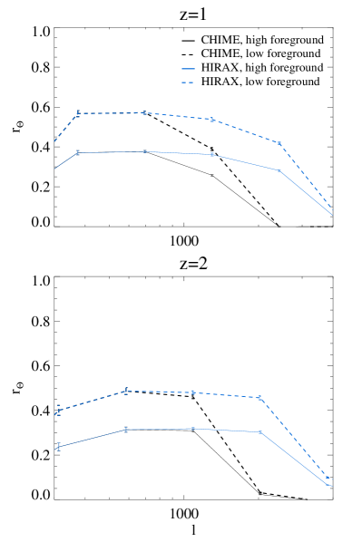
Figure 3: The correlation coefficient $r$ between kSZ distortions and kSZ templates generated from 21cm IM field. Forecasts for two instruments and different levels of foregrounds are calculated for $z=1$ (above) and $z=2$ (below).

We run six $N$-body simulations, using the $\mathrm{CUBEP}^{3}\mathrm{M}$ code Harnois-Déraps et al. (2013), each evolving $1024^{3}$ particles in a $(1.2\,\mathrm{Gpc}/h)^{3}$ box. Simulation parameters are set as: Hubble parameter $h=0.678$, baryon density $\Omega_{b}=0.049$, dark matter density $\Omega_{c}=0.259$, amplitude of primordial curvature power spectrum $A_{s}=2.139\times 10^{-9}$ at $k_{0}=0.05\;\mathrm{Mpc}^{-1}$ and scalar spectral index $n_{s}=0.968$.

	$z=1$		$z=2$
	high foreground	low foreground	high foreground	low foreground
$R_{\parallel}$ Mpc/h	15	60	10	40
	CHIME	HIRAX	CHIME	HIRAX
$k_{\perp\,\mathrm{max}}$ $h$/Mpc	0.5	1.2	0.3	0.8
$\ell_{\mathrm{min}}$	300		200

Table 1: Parameters chosen to match the conditions of 21 cm IM. $R_{\parallel}$ indicates the largest structure resolvable along LOS after foreground removal; $k_{\perp\ \mathrm{max}}$ represents the spatial resolution; $\ell_{\mathrm{min}}$, decided by the shortest baseline, indicates the largest angular scale detectable with an interferometer.

We output the simulated density fields $\delta$ at $z=1\,\&\,2$ and apply filters to match the conditions of real 21cm IM surveys:

$$\delta^{\mathrm{IM}}(\bm{k})=\delta(\bm{k})H(k_{\perp\,\mathrm{max}}-k_{\perp})W(k_{\parallel})H(\ell-\ell_{\mathrm{min}})$$ (12)

where the Heaviside Function $H(k_{\perp\,\mathrm{max}}-k_{\perp})$ describes the angular resolution of the survey:

$$H(k_{\perp\,\mathrm{max}}-k)=\left\{\begin{array}[]{ll}1,&k\leq k_{\perp\,\mathrm{max}}\\ 0,&k>k_{\perp\,\mathrm{max}}\end{array}\right.,$$

the high pass filter $W(k_{\parallel})$ indicates the loss of information due to the foregrounds:

$$W(k_{\parallel})=1-e^{k_{\parallel}^{2}R_{\parallel}^{2}/2}\,,$$

For each redshift, we consider a high foreground case based on early observations (Switzer et al., 2013) and a low foreground case from theoretical predictions (Shaw et al., 2015). The other Heaviside function $H(\ell-\ell_{\mathrm{min}})$ indicates the largest angular scale detectable with an interferometer.

$$H(\ell-\ell_{\mathrm{min}})=\left\{\begin{array}[]{ll}0,&\ell\leq\ell_{\mathrm{min}}\\ 1,&\ell>\ell_{\mathrm{min}}\end{array}\right.,$$

$\ell_{\mathrm{min}}$ is determined by the length of the shortest baseline $B_{\mathrm{min}}$, $\ell_{\mathrm{min}}\sim 2\pi B_{\mathrm{min}}/(z+1)\lambda$. We conservatively choose a shortest baseline of $\sim 20$ m.

The parameters selected for two redshifts are listed in table 1.

We calculate the kSZ template following the procedure demonstrated in Fig.1 lower panel. First, we solve for the missing large scale modes of $\delta_{\mathrm{IM}}$ with tidal reconstruction algorithm. With the reconstructed large scale density field $\delta^{\mathrm{tide}}$, we then calculate $v_{z}^{\mathrm{tide}}$ and cross correlate it with $\delta^{\mathrm{IM}}$ to get the kSZ template.

Comparing the reconstructed $v_{z}^{\mathrm{tide}}$ field with the one directly output from simulations (Fig. 2 middle panels), we can see that the large scale modes are well-reconstructed. For the modes that contributes heavily to kSZ distortions (see Fig. 2 left bottom panel), more than 70% of the information is retrieved. Fig.  2 right panels show the increased information in the momentum field template after the tidal reconstruction. KSZ signal corresponds to $k_{z}\sim 0$ modes of momentum field, for which the correlation coefficient has an obvious increase at $\ell\sim 500-2000$.

The correlation coefficients between the recovered kSZ template and actual kSZ distortions from a certain redshift bin are presented in Fig. 3. At $z=1$, the correlation coefficient can reach 0.6 before the small scale noises start to dominate, while at $z=2$, a correlation coefficient of 0.5 can be reached. Foreground level is still the dominate factor for the correlation coefficient. The correlation coefficient is reduced by 0.2 in the strong foreground case.

VI.1 Signal to noise

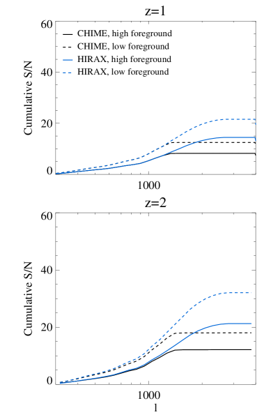
Figure 4: Cumulative S/N for the detection of kSZ signals by cross-correlating CMB from Planck with density fields from CHIME or HIRAX with $40\%$ sky coverage. The S/N is estimated for two redshift bins of 1 Gpc/$h$ centered at $z=1$ and 2 respectively.

The signal-to-noise for detecting kSZ effects can be estimated as Shao et al. (2011):

$$\frac{S}{N} = \frac{C_{\ell}}{\Delta C_{\ell}}$$

$$\simeq r\sqrt{(2\ell+1)\Delta lf_{\mathrm{sky}}}\sqrt{\frac{C_{\ell}^{\mathrm{kSZ},\Delta z}}{C_{\ell}^{\mathrm{CMB}}+C_{\ell}^{\mathrm{kSZ}}+C_{\ell}^{\mathrm{CMB},N}}},$$

where $C_{\ell}^{\mathrm{CMB}}$ is the angular power spectrum of primary CMB, $C_{\ell}^{\mathrm{CMB,N}}$ is the power spectrum of instrument noises, $C_{\ell}^{\mathrm{kSZ},\Delta z}$ is the kSZ signal from within a certain redshift bin, $r$ is the correlation coefficient defined in Eq.(3), and $f_{\mathrm{sky}}$ is the percentage of sky area covered by both CMB and 21 cm IM surveys.

We calculate $C_{\ell}^{\mathrm{CMB}}$ using CAMB Lewis et al. (2000), and estimate $C_{\ell}^{\mathrm{CMB,N}}$ with Planck data Planck Collaboration et al. (2016) at 217GHz. $C_{\ell}^{\mathrm{CMB,N}}=(\sigma_{p,T}\theta_{\mathrm{FWHM}})^{2}\,W_{\ell}^{-2}$, where $W_{\ell}=\exp[-\ell(\ell+1)/2\ell^{2}_{\mathrm{beam}}]$ is the smoothing window function, with $\ell_{beam}=\sqrt{8\ln 2}/\theta_{\mathrm{FWHM}}$. Sensitivity per beam solid angle $\sigma_{p,T}=8.7\mu\mathrm{K}_{\mathrm{CMB}}$ and effective beam FWHM $\theta_{\mathrm{FWHM}}\sim 5^{\prime}$. We assume sky coverage $f_{\mathrm{sky}}=0.4$. $C_{\ell}^{\mathrm{kSZ},\Delta z}$ is calculated within two bins of size 1200 Mpc/h, centered at redshift 1 $\&$ 2, respectively.

The cumulative S/N for CHIME+Planck and HIRAX+Planck is shown in Fig.4. The S/N at $z=2$ is higher than $z=1$ due to higher electron density. For CHIME + Planck, the resolution of CHIME determines the largest $\ell$ detectable, while for HIRAX + Planck, the resolution of Planck sets the limit. The kSZ signal is more prominent at larger $\ell$s due to the decreased strength of primary CMB, therefore increasing the resolution of facilities will largely increase the cumulative S/N.

VII Ramification

KSZ distortions come from the coupling of density and radial velocity field of different spatial scales. Although the final distortions on CMB are 2D, they contain information of radial structure due to the coupling of two fields. Different angular scale $\ell$ of kSZ tracks density field of different spatial scales, because the velocity field is large-scale dominant and contributes similarly to every $\ell$. The strength of kSZ signals at various angular scales gives measurements of the baryon content and diffuseness.

In this paper, we discuss the possibility of cross-correlating CMB with 21 cm IM field as a probe for kSZ distortions. 21 cm IM, with fast survey speed and accurate redshift information, is promising at detecting density fluctuations for large sky area and up to high redshift. The biggest challenge for the cross-correlation is the loss of large-scale information in IM due to both foregrounds and interferometer zero spacing problem. To alleviate the problem, we reconstruct the missing large-scale modes in IM from their tidal influence on the small-scale density fluctuations. With $>70\%$ of the relevant large-scale information retrieved, we are able to obtain correlation coefficients for kSZ and 21 cm fields of $0.6$ for $z=1$ and $0.5$ for $z=2$ in simulations. They are of obvious increase from the $\sim 0.1$ correlations obtained by directly using the foreground contaminated fields. For $\ell\sim 500-2000$, using CHIME+Planck, a detection of S/N$\sim 20$ can be reached for $z\sim 0.8-2.5$, while for HIRAX+Planck, a $\sim 40\sigma$ detection can be expected. This S/N can be greatly increased with instruments of higher spatial resolution or targeting at higher redshift where kSZ signals are more prominent, e.g., SPT-3G Benson et al. (2014), Advanced ACTpol Henderson et al. (2016), Simons Observatory The Simons Observatory Collaboration et al. (2018), CMB-S4 Abazajian et al. (2016), Stage II Hydrogen IM experiment Cosmic Visions 21 cm Collaboration et al. (2018), etc.

We make several approximations in the paper. We use dark matter field to assemble HI field in the analysis, which enables us to work with simple $N$ body simulations. Careful treatment should include hydrodynamic simulations which takes into account the baryonic effects (eg. Villaescusa-Navarro et al. (2018)). We ignore the foreground wedge, because it is not an intrinsic loss of information, and is believed to be removable with better understanding of instruments Liu et al. (2016). We use two boxes of 1.2 Gpc/h width output at $z=1\,\&\,2$ to represent the density field of $z=0.8-2.5$. This ignores the redshift evolution within each box. More careful work should include thinner boxes output at different redshifts. We use a uniform weight when summing over different redshifts and angular scales. The S/N could be improved if proper weights are assigned Smith et al. (2018). However, the current setups are good enough to demonstrate the feasibility of cross correlating CMB and 21 cm IM after tidal reconstruction to probe kSZ signals.

Cross-correlating the kSZ signal with 21 cm IM is promising due to its feasibility with near-term data. CHIME has started collecting data, and construction for HIRAX is underway. It is reasonable to expect our method to be testable within the next five years. This may foster understanding of stellar feedback at the scale of galaxy clusters and filaments and therefore the evolution of large-scale structures.

References

- Davé et al. (2001) R. Davé, R. Cen, J. P. Ostriker, G. L. Bryan, L. Hernquist, N. Katz, D. H. Weinberg, M. L. Norman, and B. O’Shea, ApJ 552, 473 (2001), eprint astro-ph/0007217.
- Pen (1999) U.-L. Pen, ApJ 510, L1 (1999), eprint astro-ph/9811045.
- Sołtan (2006) A. M. Sołtan, A&A 460, 59 (2006), eprint astro-ph/0604465.
- Sunyaev and Zeldovich (1972) R. A. Sunyaev and Y. B. Zeldovich, Comments on Astrophysics and Space Physics 4, 173 (1972).
- Sunyaev and Zeldovich (1980) R. A. Sunyaev and I. B. Zeldovich, MNRAS 190, 413 (1980).
- Vishniac (1987) E. T. Vishniac, ApJ 322, 597 (1987).
- Fukugita and Peebles (2004) M. Fukugita and P. J. E. Peebles, ApJ 616, 643 (2004), eprint astro-ph/0406095.
- Hand et al. (2012) N. Hand, G. E. Addison, E. Aubourg, N. Battaglia, E. S. Battistelli, D. Bizyaev, J. R. Bond, H. Brewington, J. Brinkmann, B. R. Brown, et al., Physical Review Letters 109, 041101 (2012), eprint 1203.4219.
- Shao et al. (2011) J. Shao, P. Zhang, W. Lin, Y. Jing, and J. Pan, MNRAS 413, 628 (2011), eprint 1004.1301.
- Li et al. (2014) M. Li, R. E. Angulo, S. D. M. White, and J. Jasche, MNRAS 443, 2311 (2014), eprint 1404.0007.
- Hill et al. (2016) J. C. Hill, S. Ferraro, N. Battaglia, J. Liu, and D. N. Spergel, Physical Review Letters 117, 051301 (2016), eprint 1603.01608.
- Ferraro et al. (2016) S. Ferraro, J. C. Hill, N. Battaglia, J. Liu, and D. N. Spergel, Phys. Rev. D 94, 123526 (2016), eprint 1605.02722.
- Schaan et al. (2016) E. Schaan, S. Ferraro, M. Vargas-Magaña, K. M. Smith, S. Ho, S. Aiola, N. Battaglia, J. R. Bond, F. De Bernardis, E. Calabrese, et al., Phys. Rev. D 93, 082002 (2016), eprint 1510.06442.
- Bandura et al. (2014) K. Bandura, G. E. Addison, M. Amiri, J. R. Bond, D. Campbell-Wilson, L. Connor, J.-F. Cliche, G. Davis, M. Deng, N. Denman, et al., in Society of Photo-Optical Instrumentation Engineers (SPIE) Conference Series (2014), vol. 9145 of Society of Photo-Optical Instrumentation Engineers (SPIE) Conference Series, p. 22, eprint 1406.2288.
- Xu et al. (2015) Y. Xu, X. Wang, and X. Chen, ApJ 798, 40 (2015), eprint 1410.7794.
- Newburgh et al. (2016) L. B. Newburgh, K. Bandura, M. A. Bucher, T.-C. Chang, H. C. Chiang, J. F. Cliche, R. Davé, M. Dobbs, C. Clarkson, K. M. Ganga, et al., in Ground-based and Airborne Telescopes VI (2016), vol. 9906 of Proc. SPIE, p. 99065X, eprint 1607.02059.
- Pen et al. (2012) U.-L. Pen, R. Sheth, J. Harnois-Deraps, X. Chen, and Z. Li, ArXiv e-prints (2012), eprint 1202.5804.
- Zhu et al. (2016a) H.-M. Zhu, U.-L. Pen, Y. Yu, X. Er, and X. Chen, Phys. Rev. D 93, 103504 (2016a), eprint 1511.04680.
- Zhu et al. (2016b) H.-M. Zhu, U.-L. Pen, Y. Yu, and X. Chen, ArXiv e-prints (2016b), eprint 1610.07062.
- Foreman et al. (2018) S. Foreman, P. D. Meerburg, A. van Engelen, and J. Meyers, J. Cosmology Astropart. Phys 7, 046 (2018), eprint 1803.04975.
- Di Matteo et al. (2004) T. Di Matteo, B. Ciardi, and F. Miniati, MNRAS 355, 1053 (2004), eprint astro-ph/0402322.
- Masui et al. (2013) K. W. Masui, E. R. Switzer, N. Banavar, K. Bandura, C. Blake, L.-M. Calin, T.-C. Chang, X. Chen, Y.-C. Li, Y.-W. Liao, et al., ApJ 763, L20 (2013), eprint 1208.0331.
- Planck Collaboration et al. (2016) Planck Collaboration, R. Adam, P. A. R. Ade, N. Aghanim, M. Arnaud, M. Ashdown, J. Aumont, C. Baccigalupi, A. J. Banday, R. B. Barreiro, et al., A&A 594, A8 (2016), eprint 1502.01587.
- The Simons Observatory Collaboration et al. (2018) The Simons Observatory Collaboration, P. Ade, J. Aguirre, Z. Ahmed, S. Aiola, A. Ali, D. Alonso, M. A. Alvarez, K. Arnold, P. Ashton, et al., ArXiv e-prints (2018), eprint 1808.07445.
- Abazajian et al. (2016) K. N. Abazajian, P. Adshead, Z. Ahmed, S. W. Allen, D. Alonso, K. S. Arnold, C. Baccigalupi, J. G. Bartlett, N. Battaglia, B. A. Benson, et al., ArXiv e-prints (2016), eprint 1610.02743.
- Schmidt et al. (2014) F. Schmidt, E. Pajer, and M. Zaldarriaga, Phys. Rev. D 89, 083507 (2014), eprint 1312.5616.
- Hu and et al in prep. (2018) W.-K. Hu and et al in prep. (2018).
- Harnois-Déraps et al. (2013) J. Harnois-Déraps, U.-L. Pen, I. T. Iliev, H. Merz, J. D. Emberson, and V. Desjacques, MNRAS 436, 540 (2013), eprint 1208.5098.
- Switzer et al. (2013) E. R. Switzer, K. W. Masui, K. Bandura, L.-M. Calin, T.-C. Chang, X.-L. Chen, Y.-C. Li, Y.-W. Liao, A. Natarajan, U.-L. Pen, et al., MNRAS 434, L46 (2013), eprint 1304.3712.
- Shaw et al. (2015) J. R. Shaw, K. Sigurdson, M. Sitwell, A. Stebbins, and U.-L. Pen, Phys. Rev. D 91, 083514 (2015), eprint 1401.2095.
- Lewis et al. (2000) A. Lewis, A. Challinor, and A. Lasenby, Astrophys. J. 538, 473 (2000), eprint astro-ph/9911177.
- Benson et al. (2014) B. A. Benson, P. A. R. Ade, Z. Ahmed, S. W. Allen, K. Arnold, J. E. Austermann, A. N. Bender, L. E. Bleem, J. E. Carlstrom, C. L. Chang, et al., in Millimeter, Submillimeter, and Far-Infrared Detectors and Instrumentation for Astronomy VII (2014), vol. 9153 of Proc. SPIE, p. 91531P, eprint 1407.2973.
- Henderson et al. (2016) S. W. Henderson, R. Allison, J. Austermann, T. Baildon, N. Battaglia, J. A. Beall, D. Becker, F. De Bernardis, J. R. Bond, E. Calabrese, et al., Journal of Low Temperature Physics 184, 772 (2016), eprint 1510.02809.
- Cosmic Visions 21 cm Collaboration et al. (2018) Cosmic Visions 21 cm Collaboration, R. Ansari, E. J. Arena, K. Bandura, P. Bull, E. Castorina, T.-C. Chang, S. Foreman, J. Frisch, D. Green, et al., ArXiv e-prints (2018), eprint 1810.09572.
- Villaescusa-Navarro et al. (2018) F. Villaescusa-Navarro, S. Genel, E. Castorina, A. Obuljen, D. N. Spergel, L. Hernquist, D. Nelson, I. P. Carucci, A. Pillepich, F. Marinacci, et al., ApJ 866, 135 (2018), eprint 1804.09180.
- Liu et al. (2016) A. Liu, Y. Zhang, and A. R. Parsons, ApJ 833, 242 (2016).
- Smith et al. (2018) K. M. Smith, M. S. Madhavacheril, M. Münchmeyer, S. Ferraro, U. Giri, and M. C. Johnson, ArXiv e-prints (2018), eprint 1810.13423.