A Team-Formation Algorithm
for Faultline Minimization

Abstract

In recent years, the proliferation of online resumes and the need to evaluate large populations of candidates for on-site and virtual teams have led to a growing interest in automated team-formation. Given a large pool of candidates, the general problem requires the selection of a team of experts to complete a given task. Surprisingly, while ongoing research has studied numerous variations with different constraints, it has overlooked a factor with a well-documented impact on team cohesion and performance: team faultlines. Addressing this gap is challenging, as the available measures for faultlines in existing teams cannot be efficiently applied to faultline optimization. In this work, we meet this challenge with a new measure that can be efficiently used for both faultline measurement and minimization. We then use the measure to solve the problem of automatically partitioning a large population into low-faultline teams. By introducing faultlines to the team-formation literature, our work creates exciting opportunities for algorithmic work on faultline optimization, as well as on work that combines and studies the connection of faultlines with other influential team characteristics.

1 Introduction

The problem of organizing the individuals in a given population into teams emerges in multiple domains. In a business setting, the workforce of a firm is organized in groups, with each group dedicated to a different project (Mohrman et al., 1995). In an educational context, it is common for the instructor to partition the students in her class into small teams, with team members collaborating to complete different types of assignments (Agrawal et al., 2014a, Webb, 1982, Bahargam et al., 2017, Agrawal et al., 2014b). In a government setting, elected officials are organized in committees that design and implement policies for a wide spectrum of critical issues (Fenno, 1973).

In recent years, the proliferation of online resumes and the need to evaluate large populations of candidates for on-site and virtual teams have led to a growing interest in automated team-formation (Lappas et al., 2009, Anagnostopoulos et al., 2012a, Golshan et al., 2014, Anagnostopoulos et al., 2012b, Kargar and An, 2011, An et al., 2013, Dorn and Dustdar, 2010, Gajewar and Sarma, 2012, Li and Shan, 2010, Sozio and Gionis, 2010, Agrawal et al., 2014a, Bahargam et al., 2015). Given a large pool of candidates, the general problem requires the selection of a team of experts to complete a given task. The ongoing literature has studied numerous problem variations with different constraints and optimization criteria. Examples include the coverage of all the skills required to achieve a set of goals (Lappas et al., 2009, Li and Shan, 2010, Gajewar and Sarma, 2012), smooth communication among the members of the team (Rangapuram et al., 2013, Anagnostopoulos et al., 2012a, Lappas et al., 2009, Kargar et al., 2012), the minimization of the cost of recruiting promising candidates (Golshan et al., 2014, Kargar et al., 2012), scheduling constraints (Durfee et al., 2014), the balancing of the workload assigned to each member (Anagnostopoulos et al., 2012b), and the need for effective leadership (Kargar and An, 2011).

Surprisingly, while ongoing research on team formation has studied numerous variations with different constraints, it has overlooked a factor with a well-documented impact on a team cohesion and performance: team faultlines. The faultline concept was introduced in the seminal work by Lau and Murnighan (Lau and Murnighan, 1998). Faultlines manifest as hypothetical dividing lines that split a group into relatively homogeneous subgroups based on multiple attributes (Lau and Murnighan, 1998, Meyer and Glenz, 2013). The consideration of multiple attributes is critical, as it distinguishes relevant work from the study on single-attribute faultlines, referred to as a “separation” (Harrison and Klein, 2007). The team-formation framework that we describe in this work focused on the general multi-attribute paradigm. Faultline-caused subgroups are in risk of colliding, leading to costly conflicts, poor communication, and disintegration (Bezrukova et al., 2009, Choi and Sy, 2010, Gratton et al., 2011, Jehn and Bezrukova, 2010, Li and Hambrick, 2005, Molleman, 2005, Polzer et al., 2006, Shaw, 2004, Thatcher et al., 2003).

Bridging the faultline literature with automated team-formation is challenging, as the available measures for faultlines in existing teams cannot be efficiently used for faultline optimization. For instance, many faultline measures utilize clustering algorithms to identify the large homogenous groups that create faultlines within a team (Meyer et al., 2014, Jehn and Bezrukova, 2010, Meyer and Glenz, 2013, Barkema and Shvyrkov, 2007, Lawrence and Zyphur, 2011). While such measures have emerged as the state-of-the-art, their clustering step requires a pre-existing team. Therefore, in a team-formation setting, a clustering-based measure would need to naively consider all (or an exponential number) of possible teams in order to find a faultline-minimizing solution. This brute-force approach is not applicable to even moderately-sized populations. Similarly, we cannot use any of the existing measures based on expensive (and often exponential) computations to identify the subgroups within a team (Thatcher et al., 2003, Zanutto et al., 2011, Bezrukova et al., 2009, Trezzini, 2008, Shaw, 2004, Van Knippenberg et al., 2011).

In this work, we describe the fundamental efficiency principles that a faultline measure needs to follow in order to be applicable to the automated formation of faultline-minimizing teams. We then introduce Conflict Triangles (CT): a new measure that follows these principles. The CT measure is consistent with the principles of faultline theory (Lau and Murnighan, 1998) and is founded on the extensive work on the balance of social structures (Cartwright and Harary, 1956, Easley and Kleinberg, 2010, Heider, 1958, Morrissette and Jahnke, 1967). We then use this measure as the objective function for the problem of partitioning a given population into teams, such that the average faultline score per team is minimized. We refer to this as the Faultline-Partitioning problem and formally define it in Section 4. Our work thus makes the following contributions:

1. We initiate research on the unexplored overlap between the decades of work on team faultlines and the rapidly emerging field of automated team formation.

2. We describe the fundamental efficiency principles that a faultline measure has to satisfy to be applicable to faultline-aware team-formation.

3. We present a new measure that follows these principles can thus be used for both faultline measurement and minimization. Our evaluation demonstrates the measure’s effectiveness in both tasks.

4. We formally define the Faultline-Partitioning problem, analyze its complexity, and present an efficient algorithmic framework for its solution.

By introducing faultlines to automated team-formation, our work creates exciting opportunities for algorithmic work on faultline optimization, as well as on work that combines and studies the connection of faultlines with other influential team characteristics. In Section 8, we discuss the implications of our work for practitioners in both organizational and educational settings and discuss potential directions for future work.

2 Background and Motivation

To the best of our knowledge, our work is the first to incorporate faultlines in an algorithmic framework for automated team-formation. However, our work is related to three types of research: $(i)$ algorithmic frameworks for optimizing various factors that affect the performance of a team. $(ii)$ management, psychology and sociology studies on faultlines and their effects on team outcomes, and $(iii)$ efforts measure faultlines in existing teams. Next, we discuss each of these categories in more detail.

2.1 Algorithmic work on team formation

Our previous work (Lappas et al., 2009) studied the problem of automated team-formation in the context of social networks. Given a pool of experts and a set of skills that needed to be covered, the goal there is to select a team of experts that can collectively cover all the required skills, while ensuring efficient intra-team communication. Over the last years, this work has been extended to identify a single team or a collection of teams that optimize different factors that influence a team’s performance. For example, a significant body of work has focused on incorporating different definitions of the communication cost among experts (Anagnostopoulos et al., 2012a, An et al., 2013, Dorn and Dustdar, 2010, Gajewar and Sarma, 2012, Kargar and An, 2011, Li and Shan, 2010, Sozio and Gionis, 2010, Galbrun et al., 2017). Other work has also focused on optimizing the cost of recruiting promising candidates (Golshan et al., 2014, An et al., 2013), minimizing the workload assigned to each individual team member (Anagnostopoulos et al., 2012b, 2010), satisfying scheduling constraints (Durfee et al., 2014), identifying effective leaders (Kargar and An, 2011), and optimizing the individual’s benefit from team participation (Agrawal et al., 2014a, Bahargam et al., 2015). Although all these efforts focus on optimizing various teams aspects, the work that we describe in this paper is the first to address faultline optimization. As we describe in our work, minimizing faultline potential raises new algorithmic challenges that cannot be addressed by extant algorithmic solutions.

2.2 Studies on the effects of team faultlines

For decades, researchers from various disciplines have studied the creation, operation, and performance of teams in different settings. Faultline theory was introduced by Lau and Murnighan (Lau and Murnighan, 1998). It has since been the focus of numerous follow-up works. A number of papers have studied how the existence of faultlines within a team can lead to conflict (Li and Hambrick, 2005, Choi and Sy, 2010, Thatcher et al., 2003) and affect functionality (Molleman, 2005, Polzer et al., 2006) and performance (Bezrukova et al., 2009, Thatcher et al., 2003). Motivated by the observation that the existence of faultlines does not guarantee the formation of colliding subgroups, researchers have also studied the factors that can lead to faultline activation (Pearsall et al., 2008, Jehn and Bezrukova, 2010). Further, Gratton et al. (Gratton et al., 2011) explored strategies that a leader or manager can follow to effectively handle or avoid the emergence of faultlines within a team.

2.3 Operationalizing Faultline Strength

Previous work has suggested various methods for evaluating faultlines in teams. Even though the original faultline paper by  (Lau and Murnighan, 1998) serves as the foundation of the long line of relevant literature and introduces principles that we also adopt in our work, it does not define a faultline measure. Instead, the authors lay out fundamental principles that a measure needs to follow in order to accurately evaluate the faultline strength in a given team. While these principles are appropriate for faultline measurement, they are not sufficient to ensure that a qualifying measure will also have the computational efficiency required to serve as the objective function of a scalable algorithm that has to process large populations of candidates to create teams with minimal faultlines. Computational efficiency is critical in this setting, as each of the hundreds or thousands of individuals in the given population can be represented by a point in a multidimensional space of attributes (e.g. demographics, resume information). Any team-formation algorithm would then have to efficiently navigate this space and quickly evaluate the faultline strength of many different combinations in order to identify faultline-minimizing teams. Therefore, in order to be efficiently applicable to faultline minimization, a faultline measure should follow the following two efficiency principles:

• Linear Computation: The measure should be easy to compute for a given team in polynomial time.

• Constant Updates: The measure should be easy to update in constant time if one person joins or leaves the team.

In Section 3, we introduce Conflict Triangles (CT): a new measure that provides these two characteristics. The CT measure is consistent with the principles of faultline theory (Lau and Murnighan, 1998) and is founded on the extensive work on the balance of social structures (Cartwright and Harary, 1956, Easley and Kleinberg, 2010, Heider, 1958, Morrissette and Jahnke, 1967). Next, we review the extensive literature on faultline measurement and discuss the shortcomings of extant measures in the context of the two efficiency principles that are necessary for automated team-formation.

2.3.1 State of the Art in Faultline measurement

A long line of literature has focused on identifying and measuring the strength of faultlines in existing teams. In recent years, clustering-based algorithms have emerged as the state of the art for this purpose (Meyer et al., 2014, Jehn and Bezrukova, 2010, Meyer and Glenz, 2013, Barkema and Shvyrkov, 2007, Lawrence and Zyphur, 2011). This line of work is exemplified by the 3-step Average Silhouette Width (ASW) approach proposed by (Meyer and Glenz, 2013). Given a team of individuals, the first step includes applying an agglomerative-clustering algorithm for pre-clustering the team’s members. Agglomerative clustering begins by assigning each member to its own cluster. The two most similar clusters are then iteratively joined until all points belong to the same cluster. The authors of the original paper experiment with the two most popular merging criteria: Ward’s algorithm and Average Linkage (AL). Thus, for a team with $n$ members, the joint set of results from the two alternatives yields a total of $2\times n$ possible configurations ($2$ for each possible number of clusters).

The second step focuses on computing the ASW of each possible configuration (Rousseeuw, 1987). The silhouette $s(i)$ of an individual $i$ quantifies how well a team member $i$ fits into its cluster in comparison to all other clusters and is formally defined as:

$$s(i)=\frac{b_{i}-\alpha_{i}}{max(\alpha_{i},b_{i})},$$

where $a_{i}$ is the average distance of $i$ to all other point in its cluster and $b_{i}$ is the lowest average distance of $i$ to all points in any other cluster of which $i$ is not a member. The silhouette ranges from $-1$ to $+1$, where a high value indicates that the object is well matched to its own cluster and poorly matched to others. The ASW is the average silhouette of all the team’s members.

The third step employs a post-processing method to maximize the ASW of each configuration, by temporarily moving individuals across subgroups and recomputing the ASW after each move. The move that leads to the highest increase is made permanent. The process continues until no further improvement is possible. Finally, the maximum ASW score over all configurations is reported as the strength of the team’s faultline structure.

Using ASW in automated team-formation: Previous work has repeatedly verified the advantage of the ASW measure over alternative approaches (Meyer et al., 2014, Meyer and Glenz, 2013). However, the measure cannot be efficiently used as the objective function for team-formation algorithms, as it is designed to evaluate faultline strength in existing teams and assumes that the composition of a team is part of the input. As stated earlier in this section, an appropriate measure for faultline minimization should be easy to compute in linear time and easy to update in constant time. However, Given a team of $n$ individuals, the complexity of the agglomerative-clustering step alone is $O(n^{2}logn)$ (Rokach and Maimon, 2005). There is then no guarantee on the number of reassignments that it will take for the ASW score to converge. In addition, the score cannot be updated in constant time. Instead, the deletion or addition of a member would require the new team to be re-evaluated from scratch, in order to compute the optimal ASW score.

In theory, a practitioner could consider all possible teams, evaluate their respective faultline strengths, and choose the optimum. In practice, however, this brute-force approach is not scalable and can only be applied to populations of trivial size. It can certainly not be applied to populations of hundreds or thousands of individuals, which are common in the team-formation literature (Lappas et al., 2009, Anagnostopoulos et al., 2012a, 2010). The team-partitioning task that we address in this work is considerably more computationally challenging than single-team formation. In order to use the ASW measure for this task, a practitioner would have to consider all possible partitionings of a population into fixed-size, non-overlapping teams. This is a computationally intractable process that would have to consider $O(N!)$ alternatives. Similar to the ASW measure, other clustering-based approaches are also excluded from automated team-formation due to computational efficiency (Barkema and Shvyrkov, 2007, Lawrence and Zyphur, 2011).

2.3.2 Other Faultline Measures

Similar to clustering-based approaches, most existing faultline measures are not applicable to team-formation tasks due to computational efficiency. For instance, the cost to compute the Index of Polarized Multi-Dimensional Diversity proposed by (Trezzini, 2008) grows exponentially with the number of attributes. The SGA measure by (Carton and Cummings, 2013) depends on the exhaustive evaluation of every possible partition of a given group with two or more subgroups. Similarly, the FLS measure by (Shaw, 2004) depends on the computation and averaging of all possible internal alignments and cross-product alignments of every feature with respect to the subgroups of every other feature. Given that each of these constructs has to be updated every time a person is added to or removed from a team, the FLS formula cannot be updated in constant time. The measure proposed by (Van Knippenberg et al., 2011) uses regression analysis to measure the variance of each attribute that is explained by all other attributes. Despite its advantages in a measurement setting, running multiple regressions for every candidate team is not a realistic option in a team-formation setting.

(Thatcher et al., 2003) propose a formula for computing the portion of the total variance explained by a given segmentation of a team into subgroups. Their final faultline measure $Fau_{g}$ is then defined as the score of the segmentation that maximizes the formula. However, the measure can only be applied for segmentations of two subgroups due to (i) the exhaustive nature of the search for the best split that makes the cost prohibitive in a team-formation setting, and (ii) the fact that, if we allow the number of subgroups to vary arbitrarily, the solution that maximizes the formula is to trivially assign each individual to its own subgroup. Hence, an algorithm that uses this measure to create low-faultline teams would never choose to create highly diverse teams, despite the fact that high diversity is associated with low faultlines (Lau and Murnighan, 1998). These limitations are inherited by follow up efforts that extend this measure (Zanutto et al., 2011, Bezrukova et al., 2009). The measure by (Li and Hambrick, 2005) assumes a specific attribute of interest and is not suitable for evaluating team faultlines across attributes. This is also the reason that the measure has been excluded by comparative studies of faultline measures (Meyer and Glenz, 2013).

Another relevant construct is the Subgroup Strength measure proposed by (Gibson and Vermeulen, 2003). While this measure is not designed for faultline measurement, it is relevant due to its focus on subgroups. Its creators posit that strong subgroups exist if there is high variability in the extent to which attributes overlap in the dyads within a team. Their measure is thus based on computing the pairwise similarities between the team’s members across all attributes. The team’s subgroup strength is then computed as the standard deviation over all possible member pairs. Even though this measure is not specifically designed for faultline measurement, it is easy to compute and to update, as required by the team-formation paradigm. Hence, we include this measure in our experimental evaluation in Section 5.

3 Operationalizing a Team’s Faultline Potential

We consider a pool $W$ of $n$ individual workers. Each worker $i\in{W}$ is associated with an $m$-dimensional feature vector ${\mathbf{w}}_{i}$, such that ${\mathbf{w}}_{i}(f)$ returns the value of feature $f$ for worker $i$. For each feature $f$, we create a complete signed graph $G_{f}$that includes one node for each worker in ${W}$. The sign of the edge between two nodes (workers) $(i,i^{\prime})$ is positive if they have the same value for feature $f$ (i.e. ${\mathbf{w}}_{i}(f)={\mathbf{w}}_{i^{\prime}}(f)$ ) and negative otherwise. Consider the following example:

Example 1.

We are given a pool of $3$ workers, where each worker is described by $3$ features: country of origin, gender, and undergraduate major. Our data thus consists of the following feature vectors:

$${\mathbf{w}}_{1} = [\mathrm{\tt{India}},\mathrm{\tt{Male}},\mathrm{\tt{Computer\ Science}}]$$

$${\mathbf{w}}_{2} = [\mathrm{\tt{India}},\mathrm{\tt{Male}},\mathrm{\tt{Business}}]$$

$${\mathbf{w}}_{3} = [\mathrm{\tt{China}},\mathrm{\tt{Male}},\mathrm{\tt{Chemistry}}]$$

Fig 1 shows the graphs for the three features.

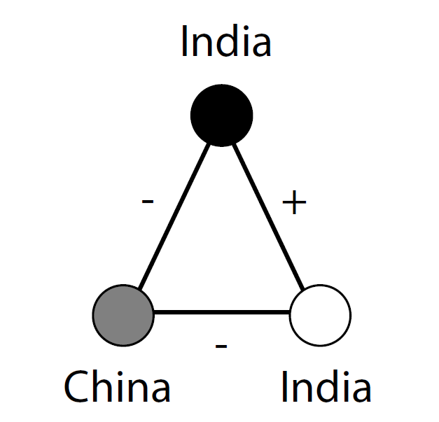
(a)

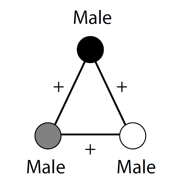
(b)

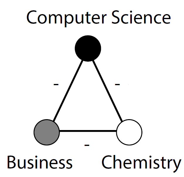
(c)

Figure 1: Triangles associated with the country of origin, gender, and educational background.

A long line of relevant literature has established the use of triangles to model social structures (Cartwright and Harary, 1956, Easley and Kleinberg, 2010, Heider, 1958, Morrissette and Jahnke, 1967). In our own setting, the triangle represents the fundamental building block of our faultline measure, as any structure that includes more members (e.g. a rectangle) can be trivially modeled via (or broken down to) triangles. The figure reveals the existence of 3 possible types of triangles among the members of the team, according to the signs on their edges: $(+,+,+)$, $(-,-,-)$, and $(-,-,+)$. By definition, $(+,+,-)$ triangles cannot exist as they would imply that 2 individuals have the same value as the third one but not the same as each other. We observe that faultlines can only appear in the presence of $(+,-,-)$ triangles that consist of one positive and two negative edges, such as the one for the country of origin feature shown in Fig 1(a). Given that faultlines can only emerge in the presence of $(+,-,-)$ triangles, we refer to these as Conflict Triangles.

A conflict triangle captures the intuition that two people from the same country are more likely to interact with each other than to the third person, thus enabling the creation of a potential faultline. On the other hand, A faultline could never occur for the gender feature (Fig 1(b)), as all three authors have the same value (Male). Similarly, since all three authors have a different value for the undergraduate major feature (Fig 1(c)), there is no faultline potential. This is consistent with faultline theory, which states that faultlines cannot emerge in the presence of perfect homogeneity or perfect diversity (Lau and Murnighan, 1998, Gratton et al., 2011).

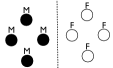
(a) High faultline potential

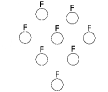
(b) No faultline potential

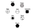
(c) No faultline potential

Figure 2: Examples of teams with high and low faultline potential.

The ability of triadic relationships to capture the perfect homogeneity/diversity principles that are mandated by faultline theory maintaints its usefulenes in a team-formation setting. Consider the example in Figure 2a. The team in the figure represents the worst-case scenario in terms of faultline potential for the gender feature: a 50-50 split between two large homogeneous groups of males (M) and females (F). Figure 2b shows an example of a team with no faultline potential for gender, as it consists exclusively of female members. Even though increased homogeneity is indeed one of the ways to reduce faultline potential, it is wrong to equate diversity with the emergence of faultlines. We demonstrate this in Figure 2c. All the members of the teams in this figure have different values with respect to the feature country of origin. We observe that, as in cases of perfect homogeneity, faultlines cannot exist in the presence of perfect diversity. This observation reveals that the task of measuring a team’s faultlines goes beyond simply measuring its diversity with respect to different features. Similarly, a team formation algorithm has to carefully balance the two states of homogeneity and diversity within a team in order to achieve a low potential for faultlines.

3.1 Feature Alignment:

The next essential step toward the design of a triangle-based faultline measure is the consideration of the alignment of conflict triangles across multiple features (Meyer and Glenz, 2013). Consider three individuals $(i,j,k)$ defined within a space of features $\mathcal{F}_{\mathcal{T}}$. Given a feature $f\in\mathcal{F}_{\mathcal{T}}$, let $\tau=<(i,j),k>$ be a conflict triangle such that ${\mathbf{w}}_{i}(f)={\mathbf{w}}_{j}(f)$ and ${\mathbf{w}}_{i}(f),{\mathbf{w}}_{j}(f)\neq{\mathbf{w}}_{k}(f)$. Let $iscon(\tau,f)$ be a function that returns 1 if $\tau$ is a conflict triangle for $f$ and 0 otherwise.

If the same conflict triangle emerges for a second feature $f^{\prime}$, we say that $\tau$ is aligned across the two features $f$ and $f^{\prime}$ (i.e. $iscon(\tau,f)=iscon(\tau,f^{\prime})=1$). Let $p(\tau,T)$ return the percentage of all available features of team $T$ for which $\tau$ is aligned (i.e. for which $\tau$ appears as a conflict triangle). Formally:

$$p(\tau,T)=\frac{|\{f\in\mathcal{F}_{\mathcal{T}}:\ iscon(\tau,f)=1\}|}{|\mathcal{F}_{\mathcal{T}}|}$$

We say that a triangle $\tau$ from team $T$ is fully aligned if it is aligned across all team features (i.e. $p(\tau,T)=1$). Then, we define the faultline potential of a given team $T$ as follows:

$$CT(T)=\sum_{\tau\in\mathcal{D}_{T}}p(\tau,T)$$ (1)

where $\mathcal{D}_{T}$ is the set of all distinct conflict triangles $<(i,j),k>$ that appear across any of the features in $T$. Our measure has a probabilistic interpretation, as it encodes the expected number of successes (conflict triangles) that we would get after $|\mathcal{D}_{T}|$ Bernoulli trials, where each trial corresponds to a different $\tau\in\mathcal{D}_{T}$ and has a success probability equal to $p(\tau,T)$. The trial for conflict triangle $\tau$ involves sampling )(uniformly at random) a feature $f$ from $\mathcal{F}_{\mathcal{T}}$ and is successful if $\tau$ is a conflict triangle for $f$. Hence, a perfectly aligned triangle would succeed for any sampled feature and would increment the team’s score by 1. Similarly, the trial for a triangle $\tau$ that is aligned over half of the team’s features would have a $50\%$ of success and would increment the team’s score by $0.5$.

The penalty that Eq. (1) assigns to each conflict triangle in the team is directly proportional to the triangle’s alignment across the team’s features.

Under this definition, the minimum faultline potential is assigned to perfectly homogeneous or perfectly diverse teams, as they both include zero conflict triangles. On the other hand, in accordance with faultline theory (Lau and Murnighan, 1998), the maximum faultline potential is assigned to teams that can be split into two perfectly homogeneous subgroups of equal size.

Learning the appropriate penalization scheme from real data: The definition given in Equation 1 intuitively applies, for each conflict triangle, a penalty that is directly proportional to the triangle’s alignment across the team’s features. We thus expect it to be a reasonable modeling choice for many domains. However, in practice, this penalization scheme may not be appropriate for a specific domain or application. Therefore, we extend our framework via by describing a methodology that allows practitioners to learn the appropriate penalization on function for their domain, based on information from existing teams in the same domain. We present the details of our technique for learning the penalization parameters in Section 6.

3.2 Efficiently computing a team’s faultline potential

The computation requires us to count the total number of conflict triangles across all features. Thus, for $T\subseteq W$, $CT(T)$ can be computed in polynomial time. For this, one has to consider all triangles appearing in the feature graphs and count how many of those are conflict triangles. The running time of the naive computation is $O(m|T|^{3})$ where $|T|$ is the size of the team and $m$ is the number of features. Next, we present a method for significantly speeding up this computation.

Given a set of workers $T\subseteq W$, and a feature $f$ that takes values $v_{1},\ldots,v_{L}$, we summarize the values of $f$ observed among the workers in $T$ via the aggregate feature vector ${r}(T,f)$ such that ${r}(T,f)[v_{j}]$ gives the number of workers in $T$ that have a value equal to $v_{j}$. We observe that these aggregate vectors can be computed in $O(m|T|)$ time by simply counting all feature values of all workers. Once the aggregate feature values have been computed, the faultline potential for each feature $f$ that takes values $v_{1},\ldots,v_{L}$ can be written as follows:

$$CT(T,f)=\sum_{j=1}^{N}{\binom{{r}(T,f)[v_{j}]}{2}}\left(|T|-{r}(T,f)[v_{j}]\right)$$ (2)

We observe that, for any feature $f$ with $L$ different possible values, the faultline potential with respect to $f$ can be computed in $O(L)$ time using the above equation. Thus, the overall faultline potential $CT(T)$ can be computed in $O(mL)$. Given that both the number of features $m$ and the number of possible values for each feature $L$ are usually small constants, this computational cost is negligible compared to the time required to create the aggregate feature values. The use of the aggregate feature vectors also allows us to update the score in constant time, as required by the second efficiency principle of faultline-aware team-formation. Specifically, if an individual $i$ joins or leaves the team, we only need to update (in $O(m)$) the number of conflict triangles that are due to the aggregate counts that change due to the addition or removal of $i$.

4 The Faultline-Partitioning Problem

In this section, we formally define the Faultline-Partitioning problem, i.e., the problem of partitioning a set of workers $W$ into $\ell$ teams of equal size such that the total faultline potential score across teams is minimized. We show that this problem is not only NP-hard to solve, but also NP-hard to approximate within any bounded approximation factor, unless $\text{P}=\text{NP}$. Then, in Section 4.1, we present an efficient heuristic algorithm for its solution.

First, we extend the notion of faultline potential to a collection of teams. For any partitioning ${\mathbf{T}}=\{T_{1},T_{2},\cdots,T_{\ell}\}$ of workers into $\ell$ teams, we use $CT({\mathbf{T}})$ to denote the total faultline potential of all teams in ${\mathbf{T}}$. Formally:

$$CT({\mathbf{T}})=\sum_{i=1}^{\ell}CT(T_{i}).$$ (3)

We can thus define the Faultline-Partitioning problem as follows:

Problem 1 (Faultline-Partitioning).

Given a pool of workers ${W}$ (with $|{W}|=\ell\times k$), find a partitioning ${\mathbf{T}}=\{T_{1},T_{2},\cdots,T_{\ell}\}$ of the workers $W$ into $\ell$ teams of size $k$ such that $CT({\mathbf{T}})$ is minimized.

Next, we proceed to analyze the hardness of the Faultline-Partitioning problem. Our results apply for the more general problem of partitioning a population into teams with specific but possibly different sizes.

Theorem 1.

The Faultline-Partitioning problem is NP-hard to solve.

Theorem 1 implies that the Faultline-Partitioning problem cannot be optimally solved in polynomial time unless $NP=P$. Next, we provide a formal proof of this theorem.

Proof.

We present a polynomial-time reduction from the NP-Complete k-Clique Partitioning problem to our Faultline-Partitioning problem (Gary and Johnson, 1979, Rosgen and Stewart, 2007). The k-Clique Partitioning is a decision problem which asks the following question: Given a graph $H=(V,X)$, is it possible to partition the nodes of the graph into disjoint cliques of size $k$?

Given a graph $H=(V,X)$ (with $V$ nodes and $X$ edges), we first create the complement of $H$ denoted by $H^{\prime}=(V,X^{\prime})$. Clearly, any clique of size $k$ in the original graph $H$ corresponds to a set of $k$ nodes with no edges among them in $H^{\prime}$.

For our reduction, every node $i\in V$ will correspond to a worker for our problem. Also, we will interpret each edge in $H^{\prime}$ as an agreement (“+”) and each missing edge as a disagreement (“-”). Then, for every edge $(i,i^{\prime})$ in $H^{\prime}$, we create a feature $f_{(i,i^{\prime})}$ and then construct the corresponding feature graph $G_{f_{(i,i^{\prime})}}$ that contains one positive edge connecting nodes $i$ and $i^{\prime}$, while all other edges, connecting all pairs of nodes, are negative. Fig 3 shows how an example graph $H$ with three edges is transformed into three feature graphs.

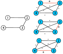
Figure 3: Graph $\widehat{H}$ (in gray) and its feature graphs for the corresponding Faultline-Partitioning problem

Now consider the optimal solution to this instance of the Faultline-Partitioning problem. Since the size of each team is fixed ($k$), it is easy to see that each edge of $H^{\prime}$ that falls within one team creates $(k-2)$ conflict triangles. This implies that the optimal solution is the one that minimizes the total number of edges that fall within the partitions. More specifically, the optimal solution has a faultline potential equal to zero if and only if there exists a partitioning of the nodes in $H^{\prime}$ with no edge inside the partitions which further corresponds to a partitioning of the nodes in $H$ into cliques. ∎

Corollary 1.

The Faultline-Partitioning problem is NP-hard to approximate within any factor.

Proof.

We will prove the hardness of approximation of Faultline-Partitioning by contradiction. Assume that there exists an $\alpha$-approximation algorithm for the Faultline-Partitioning problem. Then if ${\mathbf{T}}^{\ast}=\{T_{1}^{\ast},T_{2}^{\ast},\cdots,T_{\ell}^{\ast}\}$ is the partitioning with lowest faultline potential and ${\mathbf{T}}^{{\mathcal{A}}}=\{T_{1}^{{\mathcal{A}}},T_{2}^{{\mathcal{A}}},\cdots,T_{\ell}^{{\mathcal{A}}}\}$ is the solution output by this approximation algorithm, it will hold that $CT({\mathbf{T}}^{{\mathcal{A}}})\leq\alpha CT({\mathbf{T}}^{\ast})$. If such an approximation algorithm exists, then this algorithm can be used to decide the instances of the k-Clique Partitioning problem, for which the optimal solution has a faultline potential equal to 0. However, this contradicts the proof of Theorem 1, which indicates that these problems are also NP-hard. Thus, such an approximation algorithm does not exist. ∎

4.1 The FaultlineSplitter algorithm

In this section, we present an algorithm for the Faultline-Partitioning problem. We refer to the algorithm as FaultlineSplitter and provide the pseudocode in Algorithm 1. The Python implementation of the algorithm is available online .

The algorithm starts with a random partitioning of the input population into $\ell$ equal-size groups and then reassigns individuals to teams in an iterative fashion until the faultline potential of the obtained partitions does not improve across iterations.

1:Input: Set of workers $W$ with $m$ features and the number of desired partitions $\ell$.

2:Output: Partitioning ${\mathbf{T}}=\{T_{1},T_{2},\ldots,T_{\ell}\}$

3:Randomly partition $W$ into ${\mathbf{T}}=\{T_{1},\ldots,T_{\ell}\}$

4:while  $CT({\mathbf{T}})$ has not converged  do

5:     ${\mathbf{c}}=$ AssignCosts $(W,{\mathbf{T}})$

6:     ${\mathbf{T}}$ = ReassignTeams$\left({\mathbf{T}},{\mathbf{c}}\right)$

7:return ${\mathbf{T}}$

Algorithm 1 The FaultlineSplitter algorithm.

In each iteration, the algorithm starts with a partitioning of the set $W$ into $\ell$ groups and forms a new assignment with (ideally) a lower faultline potential score. This is done by executing two functions: AssignCosts and ReassignTeams. The AssignCosts function returns a cost associated with the assignment of every individual to every team; i.e., ${\mathbf{c}}(i,T_{j})$ is the cost of assigning individual $i$ into team $T_{j}$. These costs are used by ReassignTeams to produce a new assignment of individuals to teams – always guaranteeing that the teams are of equal size. Next, we describe the details of these the two main routines of FaultlineSplitter.

The AssignCosts routine: This routine, assigns to every worker $i$ and team $T_{j}$ cost ${\mathbf{c}}(i,T_{j})$, which is the cost of assigning worker $i$ to team $T_{j}$. In order to compute these costs, AssignCosts considers the current teams in ${\mathbf{T}}$ as a baseline to evaluate if the assignment of worker $i$ to team $T_{j}$ can lead to fewer conflict triangles. Thus, an intuitive definition of cost is the number of conflict triangles that $i$ incurs when he joins $T_{j}$. This is equal to $CT(T_{j}\cup\{i\})$ if $i\not\in T_{j}$ and $CT(T_{j})$ if $i\in T_{j}$.

We observe that, if worker $i$ already belongs to team $T_{j}$, the reassignment is not going to change the size of the resulting team. However, if $i\not\in T_{j}$ the assigning $i$ to $T_{j}$ creates a team of size $(k+1)$. This is problematic, since the number of conflict triangles in teams of size $k$ is not comparable to that in teams of size $(k+1)$. This can be resolved by introducing a normalization factor which measures the maximum possible number of conflict triangles in a team of a fixed size. Formally, for a team of size $k$, we use $\Delta_{k}$ to denote the maximum possible number of conflict triangles that can emerge in the team across all features. Now, we compute the cost function as follows:

$${\mathbf{c}}(i,T_{j})=\begin{cases}CT(T_{j}\cup\{i\})/\Delta_{k}&\text{if\ }i\not\in T_{j}\\ CT(T_{j})/\Delta_{k+1}&\text{if\ }i\in T_{j}\end{cases}$$ (4)

Running time: Note that computing all three cost functions can be done in $O(m|W|)$ using the aggregate feature vectors as discussed in Section 3.2.

The ReassignTeams routine: ReassignTeams takes as input a current a cost of assigning each one of the $n$ individuals into each one of the $\ell$ teams and outputs a new partition of the individuals into $\ell$ equal-size groups. The algorithm, views this partitioning problem as a minimum weight $b$-matching problem (Burkard et al., 2012) in a bipartite graph, where the nodes on the one side correspond to $n$ individuals and the nodes on the other side correspond to $\ell$ teams. In this graph, there is an edge between every individual $i$ and team $T_{j}$. The weight/cost of this edge is, for example, ${\mathbf{c}}(i,T_{j})$ – computed as described above. Finding a good partition then translates into picking a subset of the edges of the bipartite graph, such that the selected edges have a minimum weight sum, every individual in the subgraph defined by the selected edges has degree $1$, and each team has degree $k$. This would mean that every worker is assigned to exactly one cluster and every cluster has exactly $k$ members. This is a classical $b$-matching problem that can be solved in polynomial time using the Hungarian algorithm (Burkard et al., 2012, Kuhn, 1955).

Variable-size partitioning: It is important to point out that our algorithm can be easily modified to partition a population into teams of fixed but possibly different sizes. The ReassignTeams routine in our algorithm computes a new assignment of individuals to teams by solving a minimum weight b-matching problem in a bipartite graph where nodes on the right represent individuals and nodes on the left represent the available spots/positions in each team. This setup gives us the flexibility to choose the number of available spots in each team. In fact, this is how the algorithm enforces equal-size teams in our current implementation.

Computational speedups: Computing the new partition using the Hungarian algorithm, requires $O(n^{3})$ time. This is a computationally expensive operation, especially since this step needs to be completed in each iteration of FaultlineSplitter. In order to avoid this computational cost, we solve the bipartite $b$-matching problem approximately using a greedy heuristic that works as follows: in each iteration the edge $(i,T_{j})$ with the lowest cost ${\mathbf{c}}(i,T_{j})$ is selected, and worker $i$ is assigned to the $j$-th team $T_{j}$; this assignment only takes place if: $1)$ worker $i$ is not assigned to any team in an earlier iteration, and $2)$ the $j$-th team has less than $k$ workers so far (i.e., if it has not reached the desired team size). This is repeated until all the workers are assigned to a team.

To find the minimum cost edge in each iteration we need to sort all edges with respect to their costs and then traverse them in this order. Since there are $O(n\ell)$ edges, the running time of this greedy alternative is $O(n\ell\log(n\ell))$ per iteration.

5 Experiments

In this section, we describe the experiments that we performed to evaluate our methodology.

5.1 Datasets

Adult: The Adult dataset is a census dataset from UCI’s machine learning repository. It contains information on $32,561$ individuals; the features in the data are age, work class, education, marital status, occupation, relationship, race, sex, capital-gain, capital-loss, hours-per-week, and native country . We convert non-categorical features to categorical features as follows: for age and hours-per-week we bin their values into buckets of size $10$. Also, we convert both capital-gain and capital-loss into binary features depending whether their value is equal to zero or not.

Census: The Census dataset is extracted from the US government’s ”Current Population Survey” . We focused on the most recent collected data from the year $2014$. Our dataset contains census information on $200,469$ individuals. The dataset includes the following features: marital status, gender, education, race, country, citizen, and army.

DBLP: The DBLP dataset is created by using the latest snapshot of the DBLP website and filtering only authors that published papers on tier-1 and tier-2 computer science (NLP, IR, DM, DB, AI, Theory, Networks) conferences and journals . Although the only known attribute in the raw dataset is the country of origin, we extracted the following features for each of the $57,972$ authors, based on their publications: number of years active, primary area of focus (based on number of publications),average number of publications in ten years, and total number of publications. We also computed a quality feature for each author, by giving her 2 points for each paper published in a top-tier conference and 1 point for all other papers. We bin both the total number of publications and the average number of publications into buckets of size $10$, and bin the quality score into buckets of size $5$.

BIA660: This dataset is collected from entry surveys taken by all students who take the Analytics course offered by one of the authors of this paper. The data was collected during 6 different semesters and includes data from 502 graduate students. It consists of 85 teams, with an average of 5.9 students per team. For each student, the dataset includes the major of the degree they were pursuing at the time of the data collection, the major of their bachelor’s degree, gender, country, and a self-assessment of her level with respect to machine learning, analytics, programming, and experience with team projects. The assessments are given on a scale from 0 (no experience) to 3 (very experienced). For each team, we also have its performance (on a scale of 0 to 100) on a collaborative, semester-long project that accounts for $70\%$ of the entire grade, as well as the average satisfaction level (on a scale of 0 to 7) of the team’s members with the way the team operated. For each team we computed tension (bad triangles) for each team across all features.

Synthetic-1: In order to control the number of conflict triangles in our data, we have developed a method to create synthetic datasets given a target percentage of conflict triangles. First, we assume that our pool of workers $W$ is going to consist of a single feature which can only take $3$ different values $X$, $Y$, and $Z$. Let’s define $x$, $y$, $z$ to be the number of data points with these values respectively. Now, it is clear that ${\mathcal{N}}(W)=x\times y\times z$. On the other hand, given that total number of workers is $n$ we have $x+y+z=n$. Note that if the value of $x$ is given, we can use these equations to compute the value of $y$ and $z$ as well. To create our datasets, we try different values of $x$ and then we solve for variables $y$ and $z$. Then, we randomly partition workers into three groups of size $x$, $y$, and $z$ and assign the value $X$, $Y$, and $Z$ to them respectively.

Synthetic-2: In order to compare different faultline measures –ASW, Subgroup Strength (SS), and our CT measure– we generate a dataset as follows. We consider three features: Race (Asian, White, Black, Native American), Country (USA, China, England, France), and Education (High-school, Undergraduate, Graduate). Then, given a team size $TS$ and a number of subgroups $SN$, we generate $100$ teams that include $TS$ individuals divided into $SN$ completely homogeneous subgroups. Within each subgroup, all individuals have the same value for each feature $F$. This value $V$ is selected with a probability that is inversely proportional to the number of subgroups in the team that has already been assigned $V$ for this feature. This process allows us to create perfectly homogenous groups that are highly dissimilar from each other. We repeat the process for $TS\in\{4,8,16,32,64\}$. Given a value for $TS$, we start with $SN=1$ (a perfectly homogeneous team) and double the value until $SN=TS$ (one individual per subgroup). For instance, for $TS=16$, we consider $SN\in\{1,2,4,8,16\}$. This process generates a total of $3100$ teams. Controlling the number of perfectly homogenous subgroups allows us to control diversity and simulate multiple scenarios of conflict between different types of subgroups within the team.

Statistics for the real datasets. Dataset Size Features % of conflict triangles DBLP 57,972 6 35% Adult 32,561 12 41% Census 200,469 7 44% DBLP-Aug 155 9 47% BIA660 502 8 62% Synthetic-1 400 8 8%

Discussion: Table 5.1 shows some basic statistics for our datasets. As mentioned earlier, the Synthetic-1 dataset allows us to tune the percentage of different types of triangles. The synthetic instance reported in Table 5.1 corresponds to a dataset of size $400$ with $8$ features where we set the percentage of negative and positive triangles to $8\%$ and $25\%$ respectively. Fig 4 illustrates the Cramer’s V values for all pairs of features in all datasets. Cramer’s V value is a standard measure the correlation between two categorical variables (Cramér, 2016). It has a value of $1$ when two variables are perfectly correlated and $0$ if there is absolutely no correlation. The figure illustrates that Adult and Census are similar in terms of feature correlation. Specifically, we observe a small correlation for the majority of the features and only a couple of them with high correlations. On the other hand, DBLP exhibits significantly higher correlation patterns.

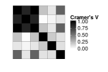
(a) DBLP

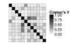
(b) Adult

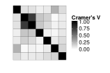
(c) Census

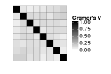
(d) Synthetic-1

(e) BIA660

(f) DBLP-Aug

Figure 4: The Cramer’s V values for all pairs of features for all datasets.

5.2 Evaluation on the Faultline-Partitioning problem

In this section, we evaluate the performance of our algorithms for the
Faultline-Partitioning problem.

Baselines: We compare our FaultlineSplitter algorithm with two baselines: Greedy and Clustering. The Greedy algorithm takes an iterative approach that creates a single team in each iteration and thus it requires $\ell$ iterations to create all $\ell$ teams. Each team is constructed as follows. First, the algorithm selects two random workers. It then continues by greedily adding the worker that minimizes the faultline score of the team. Once the size of team reaches $k$, the algorithm removes the selected members from the pool of experts and moves on to build the next team. Finally, Clustering is a clustering algorithm that tries to create equal-size partitions such that the number of positive (negative) edges within the teams is maximized (minimized) (Malinen and Fränti, 2014).

Evaluation metric: for every algorithm, we measure its performance via the faultline potential of the set of teams that it creates, as per Equation 3. Because some of our comparisons require plotting results obtained from datasets of different sizes in the same figure, we apply the following dataset-specific normalization. For a dataset of size $n$, we divide the faultline potential of a partitioning obtained for this dataset with the the total number of triangles that can be encountered in datasets of this size, i.e., ${\binom{n}{3}}$. Thus, the $y$-axis of all our plots is in $[0,1]$.

5.2.1 Varying the population size

For each dataset, we randomly select, with replacement, $100$ sets of $n$ individuals, for $n\in\{100,200,400,800,1600\}$. We then use the algorithms to partition each set into teams of size $5$. For each algorithm, we report the average faultline potential achieved over all sets for every value of $n$, along with the corresponding $90\%$ confidence intervals. The results for all three datasets are shown in Figure 5. We also report the computational time (in seconds) of each algorithm for each value of $n$ in Figure 6.

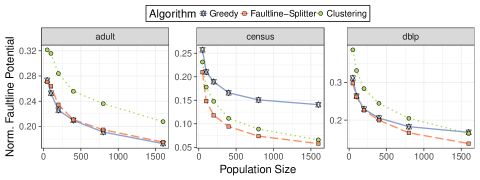
Figure 5: Faultline results for different population sizes (parameter $n$)

The first observation is that all the algorithms perform better as the size of the population increases, with the achieved normalized faultline potential values ultimately converging to a low value around $0.1$, for all datasets. An examination of the data reveals that we can confidently attribute this trend to the fact that increasing the size of the population leads to the introduction of identical or highly similar individuals (i.e. in terms of their feature values). This makes it easier to form low-faultline teams. This is not a surprising finding in real datasets, which tend to include large clusters of similar points, rather than points that are uniformly distributed within the multi-dimensional space defined by their features.

We observe that The FaultlineSplitter algorithm consistently achieves the best results across datasets, while the the Greedy algorithm outperforms Clustering in two of the three datasets DBLP and Adult. This reveals a weakness of Clustering: its inability to consistently deliver low-faultline solutions as the population becomes larger. On the other hand, the FaultlineSplitter algorithm does not exhibit this weakness, emerging as both the most stable and effective approach. Finally, as in the previous experiment, the algorithms exhibit a negligible variation over the different samples that we considered for each value of the parameter.

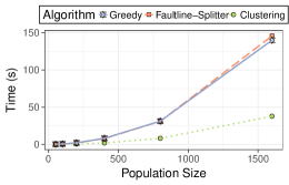
Figure 6: Running times for different population sizes (parameter $n$)

With respect to computational time, Figure 6 verifies that FaultlineSplitter can scale to large population sizes. Using the Census dataset, we observe that, even for the largest population of $1600$ individuals, the algorithm computed the solution in less 2 minutes. In fact, its speed was nearly identical to that of the greedy heuristic. Finally, while the Clustering algorithm emerges as the fastest option, this comes at the cost of inferior solutions (i.e. teams with higher faultline potential), as we demonstrated in Figure 5.

5.2.2 Varying the team size

For this experiment, we set the size of the population of individuals to $|W|=800$. For each real dataset, we randomly select $100$ populations, of $800$ individuals each, with replacement. We then use the algorithms to partition each population into teams of size $k$, for $k\in\{3,4,5,\cdots,20\}$. For each algorithm, we report the average normalized faultline potential achieved over all population for every value of $k$, along with the corresponding $90\%$ confidence intervals. The results for Adult, Census and DBLP datasets are shown in Fig 7.

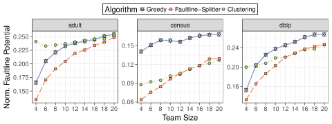
Figure 7: Faultline results for different team sizes (parameter $k$)

We observe that the FaultlineSplitter algorithm had the overall best performance across datasets. We observe that its advantage wanes as the value of $k$ increases. This can be explained by the fact that asking for larger teams makes the problem harder, as it requires the inclusion of additional individuals and thus makes it harder to avoid the introduction of conflict triangles into the team. This explanation is also consistent with the fact that the performance of the two algorithms tends to decrease as $k$ becomes larger. A second observation is that the Greedy algorithm is consistently outperformed by both FaultlineSplitter and Clustering. This demonstrates the difficulty of the Faultline-Partitioning problem and the need for sophisticated partitioning algorithms that go beyond greedy heuristics. Finally, as shown in the figure, we observe that the standard deviations for all algorithms were consistently negligible, bolstering our confidence in the reported findings.

5.2.3 Varying the number of conflict triangles

The purpose of this experiment is to evaluate the algorithm on populations with different potential for faultlines. While random samples obtained from our real-world datasets differ trivially in terms of the percentage of conflict triangles, we can engineer synthetic data to obtain datasets with different number of conflict triangles. To conduct this experiment, we use the Synthetic-1 dataset described in Section 5.1. We consider populations of $400$ individuals and set the team size equal to $5$. The results are shown in Fig 8. The plot verifies that finding low-faultline teams becomes harder as the population’s inherent potential for such faultlines increases. However, the FaultlineSplitter algorithm consistently outperforms the other methods. In fact, the gap between the two algorithms increases as the number of conflict triangles in the population increases. This demonstrates the superiority of the FaultlineSplitter algorithm over the other approaches in terms of searching the increasingly smaller space of low-faultline solutions.

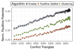
Figure 8: Performance of all algorithms for synthetic datasets with different number of bad triangles ($400$ workers, teams of size $5$ and $10$ features)

5.3 Faultline Measurement in existing teams

In this section, we compare three alternative options for faultline measurement in existing teams: the proposed CT measure, the ASW by (Meyer and Glenz, 2013), and the Subgroup Strength (SS) measure by (Gibson and Vermeulen, 2003). We select the ASW due to its status as the state-of-the-art, even though, as we discussed in detail in Section 2, it is not appropriate for the Faultline-Partitioning problem that is the main focus of our work. We select the SS measure because it combines the simplicity and computational efficiency required for the Faultline-Partitioning problem with competitive results in previous benchmarks (Meyer and Glenz, 2013).

5.3.1 A Comparison on Synthetic Teams

For this study, we use the Synthetic-2 dataset which, as we describe in Section 5.1, includes teams of various sizes and subgroup composition. First, we group the teams according to size. We then use each of the three faultline measure to evaluate the teams in each group. Finally, we compute the Pearson Correlation Coefficient (PCC) between every pair of measures. We present the results in Figure 9a. Then, in Figure 9b we report the average computational time needed to compute the score of each team for each of the three measures.

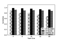
(a) Pairwise Correlation of Faultline Measures

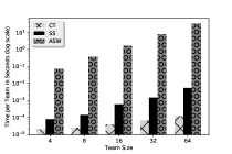
(b) Mean Computational Time

Figure 9: A comparison of the ASW, Conflict Triangles (CT), and Subgroup Strength (SS) faultline measures on the Synthetic-2 dataset.

The first observation from Figure 9a is that all three measures report similar scores across team sizes, with the pairwise PCC over $0.65$. Hence, while the three measures follow different measurement paradigms, their results tend to be consistent. However, the bars also reveal that the correlation between SS and CT measures was the highest among all possible measure-pairs. In fact, the observed PCC value for this pair was consistently around $0.9$, revealing near-perfect correlation. This is intuitive if we consider the nature of the two measures: the conflict triangles counted by the CT measure include, by definition, a pair of team members that are also identified as “overlapping” by the SS measure. A key difference between the two measures is that CT does not consider all-positive triangles (i.e. a triplet of team members with the same value for a feature, see Fig. 1b), while SS would consider all 3 dyads in such a triangle as overlaps. However, the results reveal that this difference does not significantly differentiate the results of the two measures, possibly due to the fact that SS does not follow the CT’s counting paradigm and, instead, aggregates overlap sums via the standard deviation.

With respect to computational time, Figure 9b verifies the theoretical analysis that we presented in Section 2. The y-axis represents the average time (in seconds) required to compute the score for a team, in log scale. As we discussed in detail in Section 4, any algorithm for the Faultline-Partitioning problem has to quickly consider a large number of candidate teams in order to efficiently locate (or approximate) the best possible partitioning. We observe that ASW is orders of magnitude slower than the other two measures, with the gap growing rapidly with the size of the teams. In addition, while the SS and CT measures can be easily updated in constant time as the algorithm makes small changes to the team’s roster, this is not the case for ASW. In short, while ASW may indeed be a competitive option for faultline measurement, our analysis and experiments verify that it is not a good candidate for faultline-optimization problems, such as the one that we study in this work. Out of two fastest measures, CT displays a clear advantage over SS. We observe that it is several times faster and, as in the case of ASW, the gap grows rapidly with the size of the population. The results verify the effectiveness of our methodology for computing CT, which we discuss in detail in Section 3.2. They also demonstrate that, while two measures might satisfy the efficiency principles that are necessary for efficient faultline-minimization in teams, one of the two can still have a significant computational advantage that makes it more appropriate for large populations.

5.3.2 A Comparison on Real Teams

For this study we use the BIA660 dataset, which includes two outcomes: (i) the team’s performance (represented by its grade) and (ii) the average satisfaction of the team’s members with their overall collaborative experience. In Figures 10a and  10b we visualize the performance of each team against its corresponding CT, SS, and ASW scores. We observe that performance has a strong negative association with the CT and SS scores, as demonstrated by the slope of the line. In contrast, the corresponding line for the ASW measure is nearly parallel to the x-axis, suggesting a lack of correlation. This finding is verified by the Pearson Correlation Coefficient (PCC) values for the CT, SS, and ASW measures, which were $-0.21$, $-0.23$ and $-0.04$, respectively. Note that a negative correlation is intuitive, as it means that lower faultlines are associated with higher performance.

In Figures 10c and  10d we visualize the satisfaction of each team against its corresponding CT, SS, and ASW scores. The results are consistent with the performance analysis: satisfaction exhibits a strong negative association the CT measure, while its association with ASW is very weak. In fact, the correlation of satisfaction with CT and SS appears to be even stronger than that of the team’s performance. Again, these findings are verified by the PCC values for the CT, SS, and ASW measures, which were $-0.26$, $-0.34$ and $0.02$, respectively.

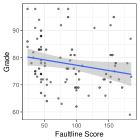
(a) Performance Vs CT

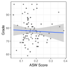
(b) Performance Vs ASW

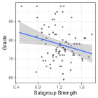
(c) Performance Vs SS

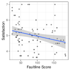
(d) Satisfaction Vs CT

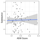
(e) Satisfaction Vs ASW

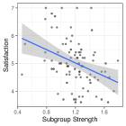
(f) Satisfaction Vs SS

Figure 10: The association of the CT, SS, and ASW measures with team performance and satisfaction.

The results verify that the teams’ overall faultline-strength, as measured by the CT measure, has a strong negative association with meaningful outcomes. Next, we demonstrate how a practitioner can examine feature-specific faultlines to identify specific features that are associated with each outcome.

Each of the two outcomes (performance and satisfaction) serves as the dependent variable in a separate regression that also includes the team’s faultline potential with respect to different features, according to the CT measure. We also consider multiple control variables that could account for part of the variance in the dependent variable. We present the results of both regressions in Table 1.

Table 1: Regression Results

	Dependent variable:
	${Grade}$	${Satisfaction}$
	${(1)}$	${(2)}$
Degree	$-10.887^{***}$	$-1.195^{***}$
	$(-3.793)$	$(-4.937)$
BS Major	$-12.821^{**}$	$-0.676$
	$(-2.580)$	$(-1.612)$
Gender	$0.106$	$0.147$
	$(0.028)$	$(0.457)$
Country	$-8.010^{***}$	$-1.121^{***}$
	$(-3.001)$	$(-4.977)$
ML Exp	$-5.428$	$-1.029^{*}$
	$(-0.841)$	$(-1.889)$
Analytics Exp	$5.233$	$-0.063$
	$(1.082)$	$(-0.155)$
Programming Exp	$-4.464$	$0.336$
	$(-0.926)$	$(0.827)$
Team Exp	$1.344$	$-0.188$
	$(0.323)$	$(-0.535)$
Average ML Exp	$0.219$	$-0.105$
	$(0.185)$	$(-1.052)$
Average Analytics Exp	$-0.241$	$-0.143$
	$(-0.205)$	$(-1.438)$
Average Prog Exp	$-1.820^{*}$	$0.014$
	$(-1.758)$	$(0.155)$
Average Team Exp	$0.898$	$0.040$
	$(0.772)$	$(0.405)$
Constant	$97.821$	$7.308^{***}$
	$(10.586)$	$(9.374)$
Observations	86	86
R2	0.313	0.467
Adjusted R2	0.200	0.379
Residual Std. Error (df = 73)	8.126	0.686
F Statistic (df = 12; 73)	2.766∗∗∗	5.327∗∗∗
Note:	The dependent variable are grade and
	satisfaction.
	t-statistics are shown in parentheses.
Significance levels:	∗p$<$0.1; ∗∗p$<$0.05; ∗∗∗p$<$0.01

The table reveals strong negative correlations of the faultline scores for the features country, BS major, and current degree with performance. This implies that the existence of potentially conflicting groups in these features can be detrimental to the team’s grade. We observe similar trends for the country and current degree features in the context of team satisfaction. Such findings can inform the instructor about the existence of potentially problematic dimensions and guide his efforts to strategically design the teams. In practice, this type of regression can be used before solving an instance of the Faultline-Partitioning problem, in order to identify the dimensions that need to be considered during the optimization. This is a critical step, as trying to solve for all possible dimensions is likely to limit the solution space and eliminate high-quality teams due to the existence of faultlines in trivial (non-influential) dimensions.

6 Generalizing the penalization scheme of aligned conflict triangles

As mentioned earlier our definition of faultline potential (summarized in Equation 1) applies, for each conflict triangle, a penalty that is directly proportional to the triangle’s alignment across the features. Our experimental results presented in Section 5.3.2 demonstrate that this penalization scheme yields a metric that is a strong predictor of a team’s success. However, one might argue that in a specific domain or application, different degrees of alignment should be penalized using a different scheme. In this section, we extend our framework by (1) demonstrating how different penalization scheme of aligned conflict triangles can be implemented, (2) describing a methodology that allows practitioners to learn the appropriate penalization scheme for their domain based on information from existing teams in the same domain, (3) studying the Faultline-Partitioning problem under a given penalization scheme.

6.1 Faultine potential with a generalized penalization scheme

Given a team $T$ with a set of features $\mathcal{F}_{T}$, we define the faultline potential of a team given a penalization scheme $g(.)$ as:

$$PCT(T,g)=\sum_{x=1}^{|\mathcal{F}_{T}|}g(x)\times aligned(x,T),$$ (5)

where $aligned(i,T)$ returns the number of conflict triangles that are aligned across exactly $x$ features in $\mathcal{F}_{T}$. The above formulation allows us to flexibly penalize the existence of aligned conflict triangles by selecting the appropriate $g(x)$ penalty for each value of $x$. Naturally, it makes sense to define $g(x)$ as an ascending function to reflect the fact that higher alignment should translate to a higher faultline potential. Note that if define $g(x)=x$, then the obtained faultine potential is equivalent to our original definition of $CT(t)$ presented in Equation 1 (module some constant).

6.2 Learning the penalization scheme

The task of learning the appropriate penalty parameters can be modeled as a supervised learning task. Each team serves as a data point in the training set. More specifically, the predictive variables are the $aligned(x,T)$ values for increasing values of $x$. The dependent variable should reflect the degree to which a team’s performance is influenced by faultlines. We compute the dependent variables using the following technique. Given a set of teams along with any success metric that encodes their outcome in a particular domain (e.g. performance, satisfaction, cohesion), we obtain the dependent variables by negating the success scores and normalizing them to have a mean equal to $0$ and a standard deviation equal to $1$. The goal is then to learn the penalty-parameters $g(x)$ that best fit the data. To achieve this, we train a linear regression to obtain the best $g(x)$ values. It is important to mention that fitting the linear regression may lead to negative $g(x)$ values. This does not create any issues, but if practitioners desire to obtain faultline potential values that are always positive, they can simply add a constant to all $g(x)$ values. This is a safe operation as it simply adds a constant value to all fautline potential values and does not affect the difference between teams’ faultline potentials. In fact, in our experiments we always add a constant value to all $g(x)$ parameters to ensure that $g(0)$ is equal to $0$. This makes the penalization scheme more interpretable as we expect the penalty of conflict-free triangles to be $0$.

If the practitioner has no access to numeric outcomes variables, we can still learn $g(x)$ as follows. The learning task can be modeled as a classification task with a binary variable that is equal $1$ for all actual teams in the data. The training data is then complemented by randomly-populated “noise” groups that do not represent actual teams. The binary dependent variable for these fake teams is $0$. In this case, the goal is to find the penalty-parameters that best differentiate between actual and noise teams. This technique builds upon the fact that in most cases, individuals (and managers) tend to form teams that have a lot degree of conflict and faultline potential.

To demonstrate the effectiveness of our proposed learning procedure, we use the BIA660 dataset as it consists of a set of teams along with two outcome scores, namely “grade” and “satisfaction”. Table 6.2 summarizes the $g(x)$ values we obtained using the techniques described above. The first two rows correspond to the $g(x)$ values obtained from the grade and satisfaction metrics. The third row corresponds to $g(x)$ values calculated from our binary classification task (without using any outcome scores). The fourth rows corresponds to $g(x)$ values obtained on a version of BIA660 dataset in which outcome score of each team is randomly sampled from the set $\{0,1\}$. This row helps verify that the results of the other rows is significant and not due to chance.

Obtained penalization schemes using the BIA660 dataset $\mathbf{g}(1)$ $\mathbf{g}(2)$ $\mathbf{g}(3)$ $\mathbf{g}(4)$ $\mathbf{g}(5)$ $\mathbf{g}(6)$ $\mathbf{g}(7)$ $\mathbf{g}(8)$ Grade 0.091 0.064 0.053 0.112 0.165 0.233 0.171 0.111 Satisfaction 0.088 0.07 0.028 0.141 0.079 0.253 0.208 0.133 Real Vs. Fake 0.068 0.099 0.079 0.061 0.115 0.184 0.223 0.171 Random -0.063 0.021 0.428 -0.041 -0.153 0.053 0.142 0.098 Frequencies 0.2% 1.5% 6.8% 12.9% 17.0% 11.6% 4.5% 0.7%

Note that the first three rows in Table 6.2 share a similar trend (and for the most part) the numbers are ascending representing that the higher degrees of alignment should be penalized more. On the other hand, we can see that the values in the last row are significantly different and do not exhibit any meaningful pattern. We can observe that the $g(x)$ values reported in the first $3$ rows, while following the expected trend, sometimes fluctuate. For example, the values of $g(8)$ are smaller than $g(7)$. This can be explained using the last row of the table which summarizes the frequencies of each degree of the alignment in the entire dataset. For instance, we can see that in the entire dataset, there are only 0.7% of triangles that can form $8$ aligned conflicts. This means, that in our learning task this value is in almost all cases set to $0$ for both successful and unsuccessful teams. Thus, the parameters learned using the linear regression are more subject to noise. In fact, if we focus only on degrees of alignments that have at least 5% presence in the data, we can see that the $g(x)$ values are more robust and conform to our expected behaviour.

6.3 Team-formation under the generalized penalization scheme

As we discussed in Section 2.3, solving the Faultline-Partitioning problem for a large group of individuals requires an operationalized notion of faultline that can be (1) computed in linear time and (2) updated in constant time when a member joins or leaves the team. Unfortunately, these two criteria may not hold for a given penalization scheme. In fact given a team $T$, computing the $PCT(T,g)$ requires a running time of $O(m|T|^{3})$. This is because our speed-up technique described in Section 3.2 can not be applied to any penalization scheme. This makes the Faultline-Partitioning problem even more challenging to solve as it becomes computationally expensive. The FaultlineSplitter algorithm can still be used to solve the Faultline-Partitioning problem given any penalization scheme, but the solution does not scale up to large population of individuals. Given that, we present some theoretical and experimental evidence to demonstrate that solving the Faultline-Partitioning problem with our original penalization scheme produces teams that are of high-quality under different penalization schemes as well. Of course, directly solving the Faultline-Partitioning problem with a given penalization scheme can produce better results, but in most cases the slight improvement can not justify the huge required computational cost.

Let us use $CT(T)$ and $PCT(T,g)$ to refer to the definition of faultline potential (according to Equation 1) and the faultline potential given a penalization scheme (according to Equation 5) respectively. Now, it is easy to show that

$$CT(T)*\max(g(x))*m\geq PCT(T,g).$$

The above equation simply states that in the worst-case scenario all $m$ features of conflicting individuals form a conflicting triangle. This is an strict upper bound for $PCT(T,g)$. Although this may not be a tight bound, it suggest that optimizing $CT(T)$ directly might be an efficient strategy for solving the Faultline-Partitioning problem under any penalization scheme.

The following experiment further demonstrates that optimizing the original faultline potential (presented in Equation 1 is quite aligned with optimizing faultline potential under a given penalization scheme. In this experiment, we have solved the Faultline-Partitioning problem on the BIA660 dataset using the penalization scheme from the first row of Table 6.2. More precisely, we ran the FaultlineSplitter algorithm to create $50$ teams of equal size. In each iteration of the algorithm, we recorded the faultline potential according to Equation 1. Figure 11 illustrates how the value of $CT(T)$ and $PCT(T,g)$ compare as the optimization proceeds. We can see that the $PCT(T,g)$ has an almost linear relationship with our original definition of faultline potential. This implies that by solving the Faultline-Partitioning problem using our original penalization scheme, we can benefit from the speed-up techniques we introduced in Section 3.2 without sacrificing the quality of the obtained teams even if a different penalization scheme is desired.

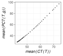
Figure 11: Comparing the faultline potential using different penalization schemes

7 Handling numeric attributes

One of the limitations of CT is that it is primarily designed for nominal attributes. Thus, numerical attributes need to be discretized into bins prior to computing the faultline score. The ability to handle multimodal data is a well-known challenge in faultline measurement. For instance, the popular ASW approach has to pre-process the data by using dummy variables to encode categorical variables as numeric. Next, we present two techniques to extend our basic CT model to deal with numerical attributes.

The first technique is based on binning, but aims to creates bins of variable length that can accurately capture the distribution of the underlying data. More precisely, a pre-processing module based on Kernel Density Estimation (KDE) could automate the discretization process and deliver dynamic segmentations that accurately capture the distribution of numeric variables (Rudemo, 1982). The resulting bins would then represent the natural groups of numeric values that are present in the given dataset.

An alternative technique that departs from the standard binning paradigm would be to use a threshold $\gamma$ to define agreement and disagreement between team members. Specifically, given a numeric feature $f$, we say two individuals $i$ and $i^{\prime}$ are in agreement iff $|{\mathbf{w}}_{i}(f)-{\mathbf{w}}_{i^{\prime}}(f)|\leq\gamma$. Otherwise, the two individuals are considered to be in a disagreement. As before, a triangle is identified as a conflict triangle with respect to feature $f$ if two of each members agree on feature $f$ and disagree with the third individual in the triangle. The problem then translates into the task of selecting an appropriate value for $\gamma$. Domain knowledge is a key factor in this effort, as each feature is likely to have its own threshold. For instance, while a difference of 2 years for the age feature is generally considered small, a difference of 2 stars in the context of the popular 5-star rating scale is far more significant. An intuitive way to set feature-specific thresholds would be to assume that two members agree on feature $f$ if the difference of their corresponding values is within 1 standard deviation of the same feature (as computed across the entire population that we want to partition into teams). A second way to tune the feature-specific thresholds is to use a validation set that includes the scores of teams for meaningful team outcomes, such as performance or satisfaction. We used such a dataset in Section 5.3.2. We can then choose the threshold values that maximize the correlation between the resulting faultline and outcomes scores.

While the above methods allow us to flexibly model (dis)agreements and address numeric attributes during the computation of conflict triangles, they do not directly model the degree of disagreement between two team members in the context of a numeric feature. For instance, a conflict triangle with two members in their 20s and one in their 30s tends to be less problematic than a triangle with two member in their 20s and one in their 60s. To address this issue, we can weigh (the disagreement in) a conflict triangle by directly using the numeric values of its members. In practice, the weight of a conflict triangle with respect to feature $f$ would then be equal to the the average absolute difference between the values of feature $f$ for the two individuals in disagreement. The CT measure would then be expressed as a weighted sum, rather than the pure number of conflict triangles in the given team. Combining this method with the two techniques that we discussed above (or with any techniques based on binning or definitions of disagreement) enables us to comprehensively extend our approach to handle numeric attributes.

8 Discussion

Our work focuses on the previously unexplored overlap between the decades of work on team faultlines and the rapidly growing literature on automated team-formation. We formally define the Faultline-Partitioning problem, which is the first problem definition that asks for the formation of teams with minimized faultlines from a large population of candidates. We present a detailed complexity analysis and introduce a new faultline-minimization algorithm (FaultlineSplitter) that outperforms competitive baselines in an experimental evaluation on both real and synthetic data.

One of the major challenges that we address in this work is finding a faultline measure that can be efficiently applied to faultline optimization. As we highlight in this paper, computational efficiency (in a practical team-formation setting) translates into two requirements that an appropriate measure should satisfy: (i) the ability to compute the faultline score of a team in linear time, and (ii) the ability to update a team’s score in constant time after small changes to the team (e.g. the removal or addition of a member). The relevant literature has described multiple operationalizations of the faultline concept. However, as we discuss in detail in Section 2, these operationalizations do not satisfy these requirements and are only appropriate for measuring faultline strength in existing teams. As such, they are not scalable enough to serve as the objective function of a combinatorial algorithm that has to process a large population and evaluate very large numbers of candidate-teams in order to find a faultline-minimizing solution. Therefore, we introduce a new measure that we refer to as Conflict Triangles (CT). The CT measure is based on the extensive literature on modeling social structures and is consistent with the fundamental principles of faultline theory by (Lau and Murnighan, 1998). In addition, CT satisfies the two efficiency requirements and is appropriate for faultline-optimization algorithms.

8.1 Implications

Our work is the first to incorporate the faultline concept into an algorithmic framework for automated team-formation. From a team-builder’s perspective, the ability to control the faultlines of teams that are automatically sampled from a large population of candidates has multiple uses. First, it allows the team builder to proactively reduce the risk of undesirable outcomes that have been consistently linked with faultlines, such as conflicts, polarization, and disintegration. Second, it provides an effective way to manage the diversity within a team. A trivial way to eliminate faultlines is to create highly homogeneous teams. However, this approach would also lead to teams that are unable to benefit from the well-documented benefits of diversity, such as innovation and increased performance (Kearney et al., 2009, Roberge and Van Dick, 2010, Van der Vegt and Janssen, 2003). In order to avoid such shortcomings, a team-builder can utilize our algorithmic framework to strategically engineer low-faultline teams without over-penalizing diversity. A characteristic example is a team that is maximally diverse; a team in which no two individuals share a common attribute. Consistent with the faultline theory by (Lau and Murnighan, 1998), our framework would recognize this as a team with the same faultline potential as a perfectly homogeneous team. We demonstrate this via examples in Figures 1 and 2.

Our team-partitioning paradigm has applications in both an organizational and educational setting. In a firm setting, the task of partitioning a workforce into teams is common. By using the proposed FaultlineSplitter algorithm, a manager can identify faultline-minimizing partitionings within the multidimensional space defined by various employee features. A regression analysis, such as the one we described in Section 5.3.2, can guide the manager’s team-building efforts by selecting specific features with potentially problematic faultlines. In a classroom setting, instructors often face the task of partitioning their students into teams for assignments and projects. As we demonstrated in our experiments, faultlines in student teams can have a strong association with meaningful outcomes, such as performance and member satisfaction. By releasing our team-partitioning software, we hope that we can automate this team-formation task and benefit both students and instructors.

8.2 Directions for Future Work

Future work could focus on algorithms that combine faultlines minimization (either as an objective function or via constraints) with other factors, such as intra-team communication, skill coverage, and recruitment cost. Such work would add to the rapidly growing literature on automated team formation, which we review in Section 2.1. We expect this to be a challenging task from an optimization perspective, as additional constraints can be hard to satisfy while trying to avoid the creation of faultlines. For instance, if the distribution of skills is strongly correlated with the population’s demographics, a homogenous team is unlikely to exhibit a diverse skillset. Hence, the ability to leverage both homogeneity and diversity will be an asset for such efforts.

The proposed FaultlineSplitter algorithm can be combined with any faultline measure that follows the efficiency principles that we describe in this work (i.e. linear computation and constant updates). Future work on such measures is essential, as existing measures are not scalable enough for optimization purposes. We make our own contribution in this direction via The CT measure that we propose in this work.

In conclusion, we hope that future efforts will be able to build on our work to address challenging problems that combine efficient algorithmic constructs for automated team-formation with the rich findings on the causes and effects of teams faultlines.

References

- Agrawal et al. (2014a) R. Agrawal, B. Golshan, and E. Terzi. Grouping students in educational settings. In Proceedings of the 20th ACM SIGKDD International Conference on Knowledge Discovery and Data Mining, KDD ’14, pages 1017–1026. ACM, 2014a. ISBN 978-1-4503-2956-9. doi: 10.1145/2623330.2623748. URL http://doi.acm.org/10.1145/2623330.2623748.
- Agrawal et al. (2014b) R. Agrawal, B. Golshan, and E. Terzi. Forming beneficial teams of students in massive online classes. In Proceedings of the First ACM Conference on Learning @ Scale Conference, L@S ’14, pages 155–156, 2014b. ISBN 978-1-4503-2669-8. doi: 10.1145/2556325.2567856. URL http://doi.acm.org/10.1145/2556325.2567856.
- An et al. (2013) A. An, M. Kargar, and M. ZiHayat. Finding affordable and collaborative teams from a network of experts. In Proceedings of the 2013 SIAM International Conference on Data Mining, pages 587–595, 2013.
- Anagnostopoulos et al. (2010) A. Anagnostopoulos, L. Becchetti, C. Castillo, A. Gionis, and S. Leonardi. Power in unity: Forming teams in large-scale community systems. In Proceedings of the 19th ACM International Conference on Information and Knowledge Management, CIKM ’10, pages 599–608, New York, NY, USA, 2010. ACM. ISBN 978-1-4503-0099-5. doi: 10.1145/1871437.1871515. URL http://doi.acm.org/10.1145/1871437.1871515.
- Anagnostopoulos et al. (2012a) A. Anagnostopoulos, L. Becchetti, C. Castillo, A. Gionis, and S. Leonardi. Online team formation in social networks. In Proceedings of the 21st International Conference on World Wide Web, WWW ’12, pages 839–848, New York, NY, USA, 2012a. ACM. ISBN 978-1-4503-1229-5. doi: 10.1145/2187836.2187950. URL http://doi.acm.org/10.1145/2187836.2187950.
- Anagnostopoulos et al. (2012b) A. Anagnostopoulos, L. Becchetti, C. Castillo, A. Gionis, and S. Leonardi. Online team formation in social networks. In Proceedings of the 21st International Conference on World Wide Web, WWW ’12, pages 839–848, New York, NY, USA, 2012b. ACM. ISBN 978-1-4503-1229-5. doi: 10.1145/2187836.2187950. URL http://doi.acm.org/10.1145/2187836.2187950.
- Bahargam et al. (2015) S. Bahargam, D. Erdos, A. Bestavros, and E. Terzi. Personalized education; solving a group formation and scheduling problem for educational content. In International Educational Data Mining Society. ERIC, 2015.
- Bahargam et al. (2017) S. Bahargam, D. Erdos, A. Bestavros, and E. Terzi. Team formation for scheduling educational material in massive online classes. arXiv preprint arXiv:1703.08762, 2017.
- Barkema and Shvyrkov (2007) H. G. Barkema and O. Shvyrkov. Does top management team diversity promote or hamper foreign expansion? Strategic Management Journal, 28(7):663–680, 2007. doi: 10.1002/smj.604. URL https://onlinelibrary.wiley.com/doi/abs/10.1002/smj.604.
- Bezrukova et al. (2009) K. Bezrukova, K. A. Jehn, E. L. Zanutto, and S. M. Thatcher. Do workgroup faultlines help or hurt? a moderated model of faultlines, team identification, and group performance. Organization Science, 20(1):35–50, 2009. doi: 10.1287/orsc.1080.0379. URL https://pubsonline.informs.org/doi/abs/10.1287/orsc.1080.0379.
- Burkard et al. (2012) R. Burkard, M. Dell’Amico, and S. Martello. Assignment Problems. Society for Industrial and Applied Mathematics, 2012.
- Carton and Cummings (2013) A. M. Carton and J. N. Cummings. The impact of subgroup type and subgroup configurational properties on work team performance. Journal of Applied Psychology, 98(5):732, 2013. doi: 10.1037/a0033593. URL https://doi.org/10.1037/a0033593.
- Cartwright and Harary (1956) D. Cartwright and F. Harary. Structural balance: a generalization of heider’s theory. Psychological review, 63(5):277, 1956. doi: 10.1037/h0046049. URL https://doi.org/0.1037/h0046049.
- Choi and Sy (2010) J. N. Choi and T. Sy. Group-level organizational citizenship behavior: Effects of demographic faultlines and conflict in small work groups. Journal of Organizational behavior, 31(7):1032–1054, 2010. doi: 10.1002/job.661. URL https://onlinelibrary.wiley.com/doi/abs/10.1002/job.661.
- Cramér (2016) H. Cramér. Mathematical Methods of Statistics (PMS-9), volume 9. Princeton university press, 2016.
- Dorn and Dustdar (2010) C. Dorn and S. Dustdar. Composing near-optimal expert teams: A trade-off between skills and connectivity. In Proceedings of the 2010 International Conference on On the Move to Meaningful Internet Systems - Volume Part I, OTM’10, pages 472–489. Springer-Verlag, 2010. ISBN 3-642-16933-3, 978-3-642-16933-5. URL http://dl.acm.org/citation.cfm?id=1947725.1947768.
- Durfee et al. (2014) E. H. Durfee, J. C. Boerkoel, Jr., and J. Sleight. Using hybrid scheduling for the semi-autonomous formation of expert teams. Future Generation Computer Systems, 31:200–212, Feb. 2014. ISSN 0167-739X. doi: 10.1016/j.future.2013.04.008. URL http://dx.doi.org/10.1016/j.future.2013.04.008.
- Easley and Kleinberg (2010) D. Easley and J. Kleinberg. Networks, Crowds, and Markets Reasoning About a Highly Connected World, volume 1. Cambridge University Press, 2010.
- Fenno (1973) R. F. Fenno. Congressmen in committees. Little, Brown, 1973.
- Gajewar and Sarma (2012) A. Gajewar and A. D. Sarma. Multi-skill collaborative teams based on densest subgraphs. In Proceedings of the 2012 SIAM International Conference on Data Mining, pages 165–176, 2012.
- Galbrun et al. (2017) E. Galbrun, B. Golshan, A. Gionis, and E. Terzi. Finding low-tension communities. In Proceedings of the 2017 SIAM International Conference on Data Mining, pages 336–344. SIAM, 2017. doi: 10.1137/1.9781611974973.38. URL https://epubs.siam.org/doi/abs/10.1137/1.9781611974973.38.
- Gary and Johnson (1979) M. R. Gary and D. S. Johnson. Computers and Intractability: A Guide to the Theory of NP-completeness. WH Freeman and Company, New York, 1979.
- Gibson and Vermeulen (2003) C. Gibson and F. Vermeulen. A healthy divide: Subgroups as a stimulus for team learning behavior. Administrative Science Quarterly, 48(2):202–239, 2003. doi: 10.2307/3556657. URL http://www.jstor.org/stable/3556657.
- Golshan et al. (2014) B. Golshan, T. Lappas, and E. Terzi. Profit-maximizing cluster hires. In Proceedings of the 20th ACM SIGKDD International Conference on Knowledge Discovery and Data Mining, KDD ’14, pages 1196–1205, New York, NY, USA, 2014. ACM. ISBN 978-1-4503-2956-9. doi: 10.1145/2623330.2623690. URL http://doi.acm.org/10.1145/2623330.2623690.
- Gratton et al. (2011) L. Gratton, A. Voigt, and T. Erickson. Bridging faultlines in diverse teams. IEEE Engineering Management Review, 39(1):80–90, 2011. ISSN 0360-8581. doi: 10.1109/EMR.2011.5729976.
- Harrison and Klein (2007) D. A. Harrison and K. J. Klein. What’s the difference? diversity constructs as separation, variety, or disparity in organizations. Academy of management review, 32(4):1199–1228, 2007. doi: 10.5465/amr.2007.26586096. URL https://doi.org/10.5465/amr.2007.26586096.
- Heider (1958) F. Heider. The Psychology of Interpersonal Relations. John Wiley & Sons, 1958. ISBN 9780898592825. URL https://books.google.com/books?id=Zh6TDmayL0AC.
- Jehn and Bezrukova (2010) K. A. Jehn and K. Bezrukova. The faultline activation process and the effects of activated faultlines on coalition formation, conflict, and group outcomes. Organizational Behavior and Human Decision Processes, 112(1):24 – 42, 2010. ISSN 0749-5978. doi: https://doi.org/10.1016/j.obhdp.2009.11.008. URL http://www.sciencedirect.com/science/article/pii/S0749597809001095.
- Kargar and An (2011) M. Kargar and A. An. Discovering top-k teams of experts with/without a leader in social networks. In Proceedings of the 20th ACM International Conference on Information and Knowledge Management, CIKM ’11, pages 985–994. ACM, 2011. ISBN 978-1-4503-0717-8. doi: 10.1145/2063576.2063718. URL http://doi.acm.org/10.1145/2063576.2063718.
- Kargar et al. (2012) M. Kargar, A. An, and M. Zihayat. Efficient bi-objective team formation in social networks. Machine Learning and Knowledge Discovery in Databases, pages 483–498, 2012. doi: 10.1007/978-3-642-33486-3˙31. URL http://dx.doi.org/10.1007/978-3-642-33486-3_31.
- Kearney et al. (2009) E. Kearney, D. Gebert, and S. C. Voelpel. When and how diversity benefits teams: The importance of team members’ need for cognition. Academy of Management Journal, 52(3):581–598, 2009. doi: 10.5465/amj.2009.41331431. URL https://doi.org/10.5465/amj.2009.41331431.
- Kuhn (1955) H. W. Kuhn. The hungarian method for the assignment problem. Naval Research Logistics Quarterly, 2:83–97, 1955. doi: 10.1002/nav.3800020109. URL https://doi.org/10.1002/nav.3800020109.
- Lappas et al. (2009) T. Lappas, K. Liu, and E. Terzi. Finding a team of experts in social networks. In Proceedings of the 15th ACM SIGKDD International Conference on Knowledge Discovery and Data Mining, KDD ’09, pages 467–476, New York, NY, USA, 2009. ACM. ISBN 978-1-60558-495-9. doi: 10.1145/1557019.1557074. URL http://doi.acm.org/10.1145/1557019.1557074.
- Lau and Murnighan (1998) D. C. Lau and J. K. Murnighan. Demographic diversity and faultlines: The compositional dynamics of organizational groups. Academy of Management Review, 23(2):325–340, 1998. doi: 10.5465/amr.1998.533229. URL https://doi.org/10.5465/amr.1998.533229.
- Lawrence and Zyphur (2011) B. S. Lawrence and M. J. Zyphur. Identifying organizational faultlines with latent class cluster analysis. Organizational Research Methods, 14(1):32–57, 2011. doi: 10.1177/1094428110376838. URL https://doi.org/10.1177/1094428110376838.
- Li and Shan (2010) C. Li and M. Shan. Team formation for generalized tasks in expertise social networks. In 2010 IEEE Second International Conference on Social Computing, pages 9–16, 2010. doi: 10.1109/SocialCom.2010.12.
- Li and Hambrick (2005) J. Li and D. C. Hambrick. Factional groups: A new vantage on demographic faultlines, conflict, and disintegration in work teams. Academy of Management Journal, 48(5):794–813, 2005. doi: 10.5465/amj.2005.18803923. URL https://doi.org/10.5465/amj.2005.18803923.
- Malinen and Fränti (2014) M. I. Malinen and P. Fränti. Balanced k-means for clustering. In Structural, Syntactic, and Statistical Pattern Recognition - Joint IAPR International Workshop, S+SSPR, pages 32–41. Springer Berlin Heidelberg, 2014.
- Meyer and Glenz (2013) B. Meyer and A. Glenz. Team faultline measures: A computational comparison and a new approach to multiple subgroups. Organizational Research Methods, 16(3):393–424, 2013. doi: 10.1177/1094428113484970. URL https://doi.org/10.1177/1094428113484970.
- Meyer et al. (2014) B. Meyer, A. Glenz, M. Antino, R. Rico, and V. González-Romá. Faultlines and subgroups: A meta-review and measurement guide. Small Group Research, 45(6):633–670, 2014. doi: 10.1177/1046496414552195. URL https://doi.org/10.1177/1046496414552195.
- Mohrman et al. (1995) S. A. Mohrman, S. G. Cohen, and A. M. Morhman Jr. Designing team-based organizations: New forms for knowledge work. Jossey Bass Business and Management Series. Jossey-Bass, 1995. ISBN 9780787900809. URL https://books.google.com/books?id=pEe5AAAAIAAJ.
- Molleman (2005) E. Molleman. Diversity in demographic characteristics, abilities and personality traits: Do faultlines affect team functioning? Group decision and Negotiation, 14(3):173–193, 2005. doi: 10.1007/s10726-005-6490-7. URL https://doi.org/10.1007/s10726-005-6490-7.
- Morrissette and Jahnke (1967) J. O. Morrissette and J. C. Jahnke. No relations and relations of strength zero in the theory of structural balance. Human Relations, 20(2):189–195, 1967. doi: 10.1177/001872676702000207. URL https://doi.org/10.1177/001872676702000207.
- Pearsall et al. (2008) M. J. Pearsall, A. P. Ellis, and J. M. Evans. Unlocking the effects of gender faultlines on team creativity: Is activation the key? Journal of Applied Psychology, 93(1):225, 2008. doi: 10.1037/0021-9010.93.1.225. URL https://doi.org/10.1037/0021-9010.93.1.225.
- Polzer et al. (2006) J. T. Polzer, C. B. Crisp, S. L. Jarvenpaa, and J. W. Kim. Extending the faultline model to geographically dispersed teams: How colocated subgroups can impair group functioning. Academy of Management Journal, 49(4):679–692, 2006. doi: 10.2307/20159792. URL https://www.jstor.org/stable/20159792.
- Rangapuram et al. (2013) S. S. Rangapuram, T. Bühler, and M. Hein. Towards realistic team formation in social networks based on densest subgraphs. In Proceedings of the 22Nd International Conference on World Wide Web, WWW ’13, pages 1077–1088, New York, NY, USA, 2013. ACM. ISBN 978-1-4503-2035-1. doi: 10.1145/2488388.2488482. URL http://doi.acm.org/10.1145/2488388.2488482.
- Roberge and Van Dick (2010) M.-É. Roberge and R. Van Dick. Recognizing the benefits of diversity: When and how does diversity increase group performance? Human Resource Management Review, 20(4):295–308, 2010. ISSN 1053-4822. doi: https://doi.org/10.1016/j.hrmr.2009.09.002. URL http://www.sciencedirect.com/science/article/pii/S1053482209000795.
- Rokach and Maimon (2005) L. Rokach and O. Maimon. Clustering methods. In Data mining and knowledge discovery handbook, pages 321–352. Springer, 2005.
- Rosgen and Stewart (2007) B. Rosgen and L. Stewart. Complexity results on graphs with few cliques. Discrete Mathematics and Theoretical Computer Science, 9(1):127–135, 2007. URL http://www.dmtcs.org/volumes/abstracts/dm090108.abs.html.
- Rousseeuw (1987) P. J. Rousseeuw. Silhouettes: A graphical aid to the interpretation and validation of cluster analysis. Journal of Computational and Applied Mathematics, 20:53 – 65, 1987. ISSN 0377-0427. doi: https://doi.org/10.1016/0377-0427(87)90125-7. URL http://www.sciencedirect.com/science/article/pii/0377042787901257.
- Rudemo (1982) M. Rudemo. Empirical choice of histograms and kernel density estimators. Scandinavian Journal of Statistics, 9(2):65–78, 1982. URL http://www.jstor.org/stable/4615859.
- Shaw (2004) J. B. Shaw. The development and analysis of a measure of group faultlines. Organizational Research Methods, 7(1):66–100, 2004. doi: 10.1177/1094428103259562. URL https://doi.org/10.1177/1094428103259562.
- Sozio and Gionis (2010) M. Sozio and A. Gionis. The community-search problem and how to plan a successful cocktail party. In Proceedings of the 16th ACM SIGKDD International Conference on Knowledge Discovery and Data Mining, KDD ’10, pages 939–948, New York, NY, USA, 2010. ACM. ISBN 978-1-4503-0055-1. doi: 10.1145/1835804.1835923. URL http://doi.acm.org/10.1145/1835804.1835923.
- Thatcher et al. (2003) S. M. Thatcher, K. A. Jehn, and E. Zanutto. Cracks in diversity research: The effects of diversity faultlines on conflict and performance. Group Decision and Negotiation, 12(3):217–241, 2003. doi: 10.1023/A:1023325406946. URL https://doi.org/10.1023/A:1023325406946.
- Trezzini (2008) B. Trezzini. Probing the group faultline concept: An evaluation of measures of patterned multi-dimensional group diversity. Quality & Quantity, 42(3):339–368, 2008. doi: 10.1007/s11135-006-9049-z. URL https://doi.org/10.1007/s11135-006-9049-z.
- Van der Vegt and Janssen (2003) G. S. Van der Vegt and O. Janssen. Joint impact of interdependence and group diversity on innovation. Journal of management, 29(5):729–751, 2003. doi: 10.1016/S0149-2063“˙03“˙00033-3. URL https://doi.org/10.1016/S0149-2063_03_00033-3.
- Van Knippenberg et al. (2011) D. Van Knippenberg, J. F. Dawson, M. A. West, and A. C. Homan. Diversity faultlines, shared objectives, and top management team performance. human relations, 64(3):307–336, 2011. doi: 10.1177/0018726710378384. URL https://doi.org/10.1177/0018726710378384.
- Webb (1982) N. M. Webb. Student interaction and learning in small groups. Review of Educational Research, 52(3):421–445, 1982. doi: 10.2307/1170424. URL https://www.jstor.org/stable/1170424.
- Zanutto et al. (2011) E. L. Zanutto, K. Bezrukova, and K. A. Jehn. Revisiting faultline conceptualization: Measuring faultline strength and distance. Quality & Quantity, 45(3):701–714, 2011. doi: 10.1007/s11135-009-9299-7. URL https://doi.org/10.1007/s11135-009-9299-7.