Electric dipole moment constraints on CP-violating light-quark Yukawas

Abstract

Nonstandard CP violation in the Higgs sector can play an essential role in electroweak baryogenesis. We calculate the full two-loop matching conditions of the standard model, with Higgs Yukawa couplings to light quarks modified to include arbitrary CP-violating phases, onto an effective Lagrangian comprising CP-odd electric and chromoelectric light-quark (up, down, and strange) dipole operators. We find large isospin-breaking contributions of the electroweak diagrams. Using these results, we obtain significant constraints on the phases of the light-quark Yukawas from experimental bounds on the neutron and mercury electric dipole moments.

1 Introduction

Electric dipole moments (EDMs) of atomic systems and elementary particles are sensitive probes of CP violation [1, 2, 3]. New sources of CP violation beyond the Standard Model (SM) are a necessary ingredient of models explaining the observed baryon asymmetry of the universe (“baryogenesis”). A particularly appealing scenario is electroweak baryogenesis (see Ref. [4] for a review), as it can potentially be probed at the LHC. In many models, electroweak baryogenesis is driven by a CP-violating phase in the Higgs-top coupling. This phase also induces an electric dipole moment (EDM) in various elementary particles and hadronic systems. Hence, experimental bounds on EDMs, for instance of the neutron, give strong constraints on new phases in the top Yukawa and naively exclude many models of baryogenesis.

On the other hand, as pointed out in Ref. [5], phases in Yukawas other than the top Yukawa are barely relevant for electroweak baryogenesis, whereas they can lead to a substantial modification of the EDM bounds. This motivates a detailed study of CP-violating contributions to all Yukawa couplings.

In Ref. [6], EDM constraints on the Yukawa couplings of the third fermion generation (top, bottom, tau) were studied. The remaining large theory uncertainty in the constraint for CP violation in the bottom Yukawa was addressed in Ref. [7], and the analysis extended to include also the charm quark. EDM constraints on the electron Yukawa were obtained in Ref. [8].

The constraints on light-quark Yukawas (up, down, and strange) were studied in Ref. [9] in the context of effective dimension-six Higgs–quark interactions. In that work, a fit was performed to one or two Yukawa couplings at a time, using hadronic EDMs induced by Barr-Zee diagrams with virtual top quarks in the loop. In the present publication, we calculate the full set of contributing two-loop diagrams induced by CP-violating phases in the light-quark Yukawas. In particular, we show that the contribution of bosonic diagrams dominates over the top-loop diagrams. Further, we show that the particular pattern of relative contributions to the electric and chromoelectric dipole operators at low energies retains the large complementarity of constraints from the neutron and mercury EDMs.

This article is organized as follows. In Sec. 2 we present the framework of our calculation, as well as the full analytic results, and the renormalization-group (RG) evolution from the electroweak to the hadronic scale. In Sec. 3 we study the numerical implications of our results for CP violation in the light-quark Yukawas, and we conclude in Sec. 4.

2 Setup and calculation

Our starting point is the SM Lagrangian with modified Yukawa couplings of the form

$$\mathscr{L}_{h-q-q} =-\frac{y^{\text{SM}}_{q}}{\sqrt{2}}\kappa_{q}\bar{q}\left(\cos\phi_{q}+i\gamma_{5}\sin\phi_{q}\right)q\,h\,,$$ (2.1)

where $h$ denotes the SM Higgs field in the broken phase, and $q$ the SM quark fields. Moreover, $y^{\text{SM}}_{q}\equiv e\,m_{q}/(\sqrt{2}s_{w}M_{W})$ is the SM Yukawa, with $e$ the positron charge, $s_{w}$ the sine of the weak mixing angle, and $M_{W}$ the $W$-boson mass, respectively. The mass of the light quark $q$ is denoted by $m_{q}$. The real parameters $\kappa_{q}\geq 0$ parameterize modifications to the absolute value of the SM Yukawa couplings, while the phases $\phi_{q}\in[0,2\pi)$ parameterize CP violation and the sign of the Yukawa. The SM value is obtained in the limit $\kappa_{q}=1$ and $\phi_{q}=0$.

In this work we are interested in constraining the phases of the light-quark Yukawas, $q=u,d,s$, via their contributions to hadronic EDMs. They are induced by the partonic low-energy effective Lagrangian [10] valid at energy scales of the order of one GeV,

$${\cal L}_{\mathrm{e}ff}=-d_{q}\,\frac{i}{2}\,\bar{q}\sigma^{\mu\nu}\gamma_{5}q\,F_{\mu\nu}-\tilde{d}_{q}\,\frac{ig_{s}}{2}\,\bar{q}\sigma^{\mu\nu}T^{a}\gamma_{5}q\,G_{\mu\nu}^{a}\,,$$ (2.2)

with $\sigma^{\mu\nu}=\tfrac{i}{2}[\gamma^{\mu},\gamma^{\nu}]$.

We calculate the contributions to this Lagrangian of the modified Yukawa couplings in Eq. (2.1) by first matching the modified SM to the effective Lagrangian

$$\mathscr{L}_{\text{eff}}=-\sqrt{2}G_{F}\,\sum_{q}\sum_{i=1,2}C_{i}^{q}O_{i}^{q}+\ldots\,$$ (2.3)

obtained by integrating out the heavy gauge bosons, the top quark, and the Higgs boson at the weak scale $\mu_{\text{ew}}\sim M_{h}=125.18\,$GeV. Here, the sum runs over all active quark fields below the weak scale ($q=u,d,s,c,b$), and the operators are defined as

$$O_{1}^{q} =\frac{ieQ_{q}}{2}\,m_{q}\,\bar{q}\sigma^{\mu\nu}\gamma_{5}q\,F_{\mu\nu}\,, O_{2}^{q} =-\frac{i}{2}\,g_{s}\,m_{q}\,\bar{q}\sigma^{\mu\nu}\gamma_{5}T^{a}q\,G^{a}_{\mu\nu}\,.$$ (2.4)

A plethora of other effective operators is generated by the matching procedure, for instance, CP-odd four-fermion operators. These other operators are either subleading or do not directly contribute to the hadronic EMDs, and are denoted by the ellipsis in Eq. (2.3).

Figure 1: The contributions to the Weinberg operator are suppressed with respect to the dipole contributions by an additional power of a light-quark Yukawa and are neglected. Here and in the following, the CP-violating Higgs coupling to the light quarks $q=u,d,s$ is denoted by a black square.

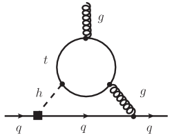
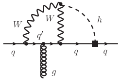
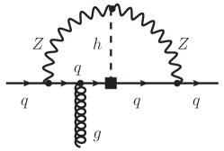
Figure 2: Sample two-loop Feynman diagrams inducing an chromoelectric dipole moment for the light quark $q=u,d,s$ through a CP-violating Higgs coupling. The label $q^{\prime}$ denotes a quark with opposite weak isospin with respect to $q$.

As a notable example, we mention that the Weinberg operator [11]

$$\begin{split}O_{3}&=-\frac{1}{3\,g_{s}}f^{abc}\,G_{\mu\sigma}^{a}G_{\nu}^{b,\sigma}\widetilde{G}^{c,\mu\nu}\,\end{split}$$ (2.5)

also receives a contribution from modified quark couplings (see Fig. 1). However, since we are interested in the light-quark Yukawa couplings, these contributions are suppressed by an additional power of a small Yukawa coupling with respect to the dipole operators (2.4). Furthermore, the dipole operators do not mix into the Weinberg operator, hence it plays no role in our calculation.

We perform the matching at the weak scale by calculating appropriate off-shell Greens functions with light external quarks, photons, and gluons. As pointed out in Ref. [12], the leading contributions arise from two-loop diagrams in the modified SM (see Fig. 2-4). In order to project all our results, we need to include one unphysical operator that vanishes by the equations of motion (e.o.m.) of the light-quark fields. It can be chosen as

$$N_{1}^{q}=m_{q}\,\bar{q}\not{D}\not{D}i\gamma_{5}q\,,$$ (2.6)

where the covariant derivative acting on quarks is defined as

$$D_{\mu}\equiv\partial_{\mu}-ig_{s}T^{a}G_{\mu}^{a}+ieQ_{q}A_{\mu}\,,$$ (2.7)

with the quark electrical charge $Q_{q}$.

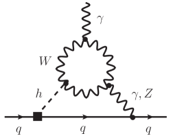
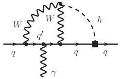
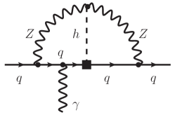
Figure 3: Sample two-loop Feynman diagrams with internal gauge bosons, inducing an electric dipole moment for the light quark $q=u,d,s$.

Many contributions to the initial conditions can be obtained, in principle, by rescaling the results for the electron EDM [8] (see also Ref. [13]). There are, however, new diagrams that appear only in the case of light-quark EDMs, since the photon does not couple to the neutrino in the case of the contributions to the electron EDM (see Fig. 3, middle panel). Note that the set of additional “non-Barr–Zee” diagrams with an internal top-quark line (see Fig. 4, right panel) are suppressed by the CKM factor $|V_{td}|^{2}\approx 7\times 10^{-5}$ and are neglected in our calculation. The corresponding diagrams with external strange quarks are suppressed by $|V_{ts}|^{2}\approx 1.5\times 10^{-3}$ and are also neglected.

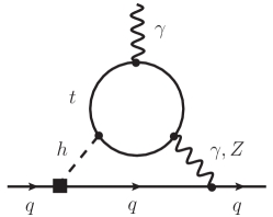
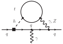
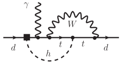
Figure 4: Sample two-loop Feynman diagrams with internal top quarks, inducing an electric dipole moment for the light quark $q=u,d,s$. Left panel: The classic “Barr–Zee” diagrams. The diagrams with an internal $Z$ boson give a substantial contribution for external down quarks. The sum of diagrams of the form shown in the middle panel vanishes (the same is true for the corresponding bosonic diagrams). Right panel: This class of diagrams with an internal top-quark line is parametrically suppressed by small CKM matrix elements and has been neglected in our calculation.

In order to display our analytic results, we decompose the Wilson coefficients as

$$\begin{split}C_{1}^{q}&=C_{1}^{q,t\gamma}+C_{1}^{q,tZ}+C_{1}^{q,W\gamma}+C_{1}^{q,WZ}+C_{1}^{q,W}+C_{1}^{q,Z}\,,\\ C_{2}^{q}&=C_{2}^{q,tg}+C_{2}^{q,W}+C_{2}^{q,Z}\,.\end{split}$$ (2.8)

The terms labeled by $t\gamma$, $tZ$, and $tg$ denote the contributions from Barr–Zee-type diagrams containing top-quark loops and an internal photon, $Z$ boson, or gluon, respectively (see Fig. 2 and Fig. 4, left panels); the terms labeled by $W\gamma$ and $WZ$ denote corresponding bosonic diagrams (see Fig. 3, left panel). The terms labeled $W$ and $Z$ denote “non-Barr–Zee” type diagrams with internal $W$ or $Z$ bosons, respectively (see Fig. 2 and Fig. 3, middle and right panels). By explicit calculation, we find

$$\begin{split}C_{1}^{q,t\gamma}=\frac{\alpha}{12\pi^{3}}\,\kappa_{q}\,\kappa_{t}\bigg{\{}&\sin(\phi_{q})\cos(\phi_{t})\,x_{th}\left[\left(2x_{th}-1\right)\Phi\left(\frac{1}{4x_{th}}\right)-2\left(2+\log x_{th}\right)\right]\\ &-\cos(\phi_{q})\sin(\phi_{t})\,x_{th}\Phi\left(\frac{1}{4x_{th}}\right)\bigg{\}}\,,\end{split}$$ (2.9)

where $x_{th}\equiv m_{t}^{2}/M_{h}^{2}$. The corresponding diagrams with gluons instead of photons (see Fig. 2, left panel) give a contribution to the initial condition of the chromoelectric dipole operator; we find

$$\begin{split}C_{2}^{q,tg}=\frac{\alpha_{s}}{32\pi^{3}}\,\kappa_{q}\,\kappa_{t}\bigg{\{}&\sin(\phi_{q})\cos(\phi_{t})\,x_{th}\left[\left(2x_{th}-1\right)\Phi\left(\frac{1}{4x_{th}}\right)-2\left(2+\log x_{th}\right)\right]\\ &-\cos(\phi_{q})\sin(\phi_{t})\,x_{th}\Phi\left(\frac{1}{4x_{th}}\right)\bigg{\}}\,.\end{split}$$ (2.10)

For the top-loop diagrams with internal $Z$ bosons we obtain

$$\begin{split}C_{1}^{q,tZ}&=\frac{\alpha}{384Q_{q}\pi^{3}s_{w}^{2}c_{w}^{2}}\kappa_{q}\kappa_{t}\left(8s_{w}^{2}-3\right)\left(4Q_{q}s_{w}^{2}\mp 1\right)\frac{x_{th}x_{tZ}}{x_{th}-x_{tZ}}\\[5.0pt] &\quad\times\bigg{\{}\sin(\phi_{q})\cos(\phi_{t})\bigg{[}\left(1-2x_{th}\right)\Phi\left(\frac{1}{4x_{th}}\right)\\[5.0pt] &\hskip 100.00015pt-2\log x_{hZ}-\left(1-2x_{tZ}\right)\Phi\left(\frac{1}{4x_{tZ}}\right)\bigg{]}\\[5.0pt] &\hskip 20.00003pt+\cos(\phi_{q})\sin(\phi_{t})\bigg{[}\Phi\left(\frac{1}{4x_{th}}\right)-\Phi\left(\frac{1}{4x_{tZ}}\right)\bigg{]}\bigg{\}}\,,\end{split}$$ (2.11)

where $x_{tZ}\equiv m_{t}^{2}/M_{Z}^{2}$ and $x_{hZ}\equiv M_{h}^{2}/M_{Z}^{2}$. Here and in the following, the upper sign corresponds to the up quark ($q=u$) and the lower sign to the down quarks ($q=d,s$). Moreover, in the remainder of this work we will assume the SM values $\kappa_{t}=1$ and $\phi_{t}=0$ for the top-quark couplings. For the bosonic Barr–Zee-type diagrams we find

$$\begin{split}C_{1}^{q,W\gamma}=&\frac{\alpha}{64\pi^{3}}\sqrt{2}\,\kappa_{q}\sin(\phi_{q})\bigg{[}\left(1+6x_{Wh}\right)\left(2+\log x_{Wh}\right)\\ &\hskip 70.0001pt+\left(7-6x_{Wh}\right)x_{Wh}\Phi\left(\frac{1}{4x_{Wh}}\right)\bigg{]}\,,\end{split}$$ (2.12)

where $x_{Wh}\equiv M_{W}^{2}/M_{h}^{2}$, and

$$\begin{split}C_{1}^{q,WZ}=&-\frac{\alpha}{512\pi^{3}s_{w}^{2}}\sqrt{2}\,\kappa_{q}\sin(\phi_{q})(x_{Zh}-1)^{-1}\bigg{(}4s_{w}^{2}\mp\frac{1}{Q_{q}}\bigg{)}\\[5.0pt] &\quad\times\bigg{[}\big{[}3-2x_{Wh}+2c_{w}^{2}(6x_{Wh}-7)\big{]}x_{Zh}\Phi\left(\frac{1}{4x_{Wh}}\right)\\[5.0pt] &\qquad+\big{[}1+18x_{Wh}-2c_{w}^{2}(1+6x_{Wh})-4x_{Zh}\big{]}\Phi\left(\frac{1}{4c_{w}^{2}}\right)\\[5.0pt] &\qquad+\bigg{(}\frac{1}{c_{w}^{2}}+2x_{Zh}-2(1+6x_{Wh})\bigg{)}\log x_{Zh}\bigg{]}\,,\end{split}$$ (2.13)

where $x_{Zh}\equiv M_{Z}^{2}/M_{h}^{2}$. The contributions to the electric and chromoelectric dipoles of diagrams with internal $Z$ bosons are equal; we find

$$\begin{split}C_{1}^{q,Z}=C_{2}^{q,Z}=&\frac{\alpha}{9216\pi^{3}s_{w}^{2}c_{w}^{2}}\sqrt{2}\,\kappa_{q}\sin(\phi_{q})x_{Zh}^{2}\bigg{[}2\big{(}1\mp 4Q_{q}s_{w}^{2}+8Q_{q}^{2}s_{w}^{4}\big{)}\\[5.0pt] &\quad\times\bigg{(}24x_{hZ}-6x_{hZ}^{2}-\big{(}4+3x_{hZ}\big{)}\pi^{2}\\[5.0pt] &\qquad\quad+\big{(}24x_{hZ}+6x_{hZ}^{2}-3x_{hZ}^{3}\big{)}\Phi\left(\frac{x_{hZ}}{4}\right)\\[5.0pt] &\qquad\quad+\big{(}24+18x_{hZ}-6x_{hZ}^{3}\big{)}\text{Li}_{2}(1-x_{hZ})\\[5.0pt] &\qquad\quad-\big{(}24x_{hZ}+6x_{hZ}^{2}\big{)}\log x_{hZ}\bigg{)}\\[5.0pt] &-12s_{w}^{2}\big{(}2Q_{q}^{2}s_{w}^{2}\mp Q_{q}\big{)}x_{hZ}^{3}\\[5.0pt] &\quad\times\bigg{(}6-\big{(}4x_{hZ}-x_{hZ}^{2}\big{)}\pi^{2}+\big{(}24-18x_{hZ}+3x_{hZ}^{2}\big{)}\Phi\left(\frac{x_{hZ}}{4}\right)\\[5.0pt] &\qquad\quad+\big{(}12-48x_{hZ}-12x_{hZ}^{2}\big{)}\text{Li}_{2}(1-x_{hZ})\\[5.0pt] &\qquad\quad+12\log x_{hZ}-\big{(}12x_{hZ}-3x_{hZ}^{2}\big{)}\log^{2}x_{hZ}\bigg{)}\bigg{]}\,.\end{split}$$ (2.14)

The corresponding contributions with internal $W$ loops are

$$\begin{split}C_{1}^{q,W}=&\pm\frac{\alpha}{2304\pi^{3}Q_{q}s_{w}^{2}}\sqrt{2}\,\kappa_{q}\sin(\phi_{q})x_{hW}\\[5.0pt] &\times\bigg{[}\pm Q_{q}\big{(}24x_{Wh}^{2}-6x_{Wh}\big{)}-18x_{Wh}\mp Q_{q}\big{(}3x_{Wh}^{2}+4x_{Wh}^{3}\big{)}\pi^{2}\\[5.0pt] &\qquad+\Big{(}18\big{(}x_{Wh}-x_{Wh}^{2}\big{)}-9\pm 3Q_{q}\big{(}8x_{Wh}^{2}+2x_{Wh}-1\big{)}\Big{)}\Phi\left(\frac{1}{4x_{Wh}}\right)\\[5.0pt] &\qquad+\Big{(}18\pm 3Q_{q}\big{(}1-4x_{Wh}^{3}-3x_{Wh}^{2}\big{)}\Big{)}\Big{(}2\text{Li}_{2}(1-x_{Wh})+\log^{2}x_{Wh}\Big{)}\\[5.0pt] &\qquad+\Big{(}18x_{Wh}\pm Q_{q}\big{(}6x_{Wh}+24x_{Wh}^{2}\big{)}\Big{)}\log x_{Wh}\bigg{]}\,\end{split}$$ (2.15)

and

$$\begin{split}C_{2}^{q,W}=&\frac{\alpha}{2304\pi^{3}s_{w}^{2}}\sqrt{2}\,\kappa_{q}\sin(\phi_{q})x_{hW}\\[5.0pt] &\times\bigg{[}\big{(}24x_{Wh}^{2}-6x_{Wh}\big{)}-\big{(}3x_{Wh}^{2}+4x_{Wh}^{3}\big{)}\pi^{2}\\[5.0pt] &\qquad+3\big{(}8x_{Wh}^{2}+2x_{Wh}-1\big{)}\Phi\left(\frac{1}{4x_{Wh}}\right)\\[5.0pt] &\qquad+3\big{(}1-4x_{Wh}^{3}-3x_{Wh}^{2}\big{)}\Big{(}2\text{Li}_{2}(1-x_{Wh})+\log^{2}x_{Wh}\Big{)}\\[5.0pt] &\qquad+\big{(}6x_{Wh}+24x_{Wh}^{2}\big{)}\log x_{Wh}\bigg{]}\,,\end{split}$$ (2.16)

where $x_{hW}\equiv M_{h}^{2}/M_{W}^{2}$. In Eqs. (2.15) and (2.16) we suppressed the explicit dependence on the CKM factors. For $q=u$, these two results should be multiplied by $|V_{ud}|^{2}+|V_{us}|^{2}+|V_{ub}|^{2}$, for $q=d$, by $|V_{ud}|^{2}+|V_{cd}|^{2}$, and for $q=s$, by $|V_{us}|^{2}+|V_{cs}|^{2}$. In all cases, the squared CKM matrix elements sum to unity to a very good approximation. Note that we neglected the tiny contributions of diagrams with internal top quarks.

To simplify the above expressions we defined $c_{w}=M_{W}/M_{Z}$ and $s_{w}=\sqrt{1-c_{w}^{2}}$. The function $\Phi(z)$ is given by [14]

$$\begin{split}\Phi(z)&=4\bigg{(}\frac{z}{1-z}\bigg{)}^{1/2}\text{Cl}_{2}\big{(}2\arcsin(z^{1/2})\big{)}\,,\\[5.0pt] \text{Cl}_{2}(\theta)&=-\int_{0}^{\theta}dx\log|2\sin(x/2)|\,,\end{split}$$ (2.17)

for $z<1$ and by

$$\begin{split}\Phi(z)&=\bigg{(}\frac{z}{z-1}\bigg{)}^{1/2}\bigg{\{}-4\text{Li}_{2}(\xi)+2\log^{2}\xi-\log^{2}(4z)+\frac{\pi^{2}}{3}\bigg{\}}\,,\\[5.0pt] \xi&=\frac{1-\big{(}\frac{z-1}{z}\big{)}^{1/2}}{2}\,,\end{split}$$ (2.18)

for $z>1$, where ${\mathrm{L}i}_{2}(x)=-\int_{0}^{x}du\,\ln(1-u)/u$ is the usual dilogarithm.

The actual calculation was performed in two independent setups, both based on self-written FORM [15] routines. The amplitudes were generated using QGRAF [16] and FeynArts [17], respectively, using the Feynman rules in background-field gauge from Ref. [18]. Both setups implement the two-loop recursion presented in Refs. [14, 19]. Needless to say that the two calculations yield identical results.

Having obtained the initial conditions of the Wilson coefficients for the operators in Eq. (2.3), we now use the one-loop renormalization group (RG) equations to evolve the Wilson coefficients from the weak scale $\mu_{\text{ew}}$ down to the hadronic scale $\mu_{\text{had}}=2\,$GeV, integrating out the bottom and charm quarks at their respective thresholds. This procedure automatically sums the large logarithms $\log(M_{h}/\mu_{\text{had}})$ to leading-logarithmic (LL) order. We follow the standard procedure and conventions described in Ref. [20].

Focusing on the light quarks $q=u,d,s$ only, the evolution from the weak scale to the hadronic scale is given by the RG equation

$$\mu\frac{d}{d\mu}C(\mu)=\gamma^{T}C(\mu)\,,$$ (2.19)

where $C(\mu)\equiv(C_{1}^{q}(\mu),C_{2}^{q}(\mu))^{T}$, and the anomalous dimension matrix is given, to leading order, by [21, 22]

$$\gamma=\frac{\alpha_{s}}{4\pi}\begin{pmatrix}\frac{32}{3}&0\\[5.0pt] \frac{32}{3}&\frac{28}{3}\end{pmatrix}\,.$$ (2.20)

Note that operators with different quark flavors do not mix at one-loop order. The contributions to the low-energy effective Lagrangian (2.2) are then given in terms of the Wilson coefficients at $\mu_{\text{had}}=2\,$GeV in the three-flavor effective theory by the relations

$$\begin{split}d_{q}(\mu)&=\sqrt{2}G_{F}\,Q_{q}e\,m_{q}\,C_{1}^{q}(\mu)\,,\\[5.0pt] \tilde{d}_{q}(\mu)&=-\sqrt{2}G_{F}\,m_{q}\,C_{2}^{q}(\mu)\,.\end{split}$$ (2.21)

3 Numerics

In this section, we evaluate our results numerically and study their impact on the neutron and mercury EDMs. Using experimental bounds, we derive constraints on the phases of the light-quark Yukawas at the end of this section. All numerical input parameters in this section are taken from Ref. [23].

The numerical size of the individual contributions to the initial conditions of the Wilson coefficients at the weak scale are

$$C_{1}^{u}(\mu_{\text{ew}}) =(-4.5+14.4)\times 10^{-5}\times\kappa_{u}\sin(\phi_{u})\,;$$ (3.1)

$$C_{1}^{q}(\mu_{\text{ew}}) =(-5.6+20.1)\times 10^{-5}\times\kappa_{q}\sin(\phi_{q})\,,\quad q=d,s\,,$$ (3.2)

where we chose $\mu_{\text{ew}}=M_{h}=125.18\,$GeV. The first terms in the brackets correspond to the top-loop contributions, see Fig. 4, left panel. The diagrams with internal photons have been calculated previously, while the diagrams with internal $Z$ bosons are included here for the first time. The second terms correspond to the previously unknown bosonic contributions, see Fig. 3. It is interesting to note that they enter with the opposite sign and dominate numerically over the fermionic contributions, similar to the case of the Higgs decay rate into two photons. For the contribution to the chromoelectric dipole operator we find

$$C_{2}^{u}(\mu_{\text{ew}}) =(-22.1+4.2)\times 10^{-5}\times\kappa_{u}\sin(\phi_{u})\,;$$ (3.3)

$$C_{2}^{q}(\mu_{\text{ew}}) =(-22.1+3.0)\times 10^{-5}\times\kappa_{q}\sin(\phi_{q})\,,\quad q=d,s\,,$$ (3.4)

The LL RG evolution of the Wilson coefficients from $\mu_{\text{ew}}=M_{h}$ to $\mu_{\text{had}}=2\,$GeV is obtained by solving Eq. (2.19) numerically. We find

$$C_{1}^{u}(\mu_{\text{had}}) =\kappa_{u}\sin(\phi_{u})(1.16\pm 0.09)\times 10^{-4}\,;$$ (3.5)

$$C_{1}^{q}(\mu_{\text{had}}) =\kappa_{q}\sin(\phi_{q})(1.45\pm 0.10)\times 10^{-4}\,,\quad q=d,s\,;$$ (3.6)

$$C_{2}^{u}(\mu_{\text{had}}) =-\kappa_{u}\sin(\phi_{u})(1.07\pm 0.23)\times 10^{-4}\,;$$ (3.7)

$$C_{2}^{q}(\mu_{\text{had}}) =-\kappa_{q}\sin(\phi_{q})(1.14\pm 0.23)\times 10^{-4}\,,\quad q=d,s\,.$$ (3.8)

The central values correspond to the values at $\mu_{\text{ew}}=M_{h}$. We estimate the theoretical uncertainty by studying the residual scale dependence; the quoted errors correspond to half the size of the interval obtained by varying the electroweak matching scale in the interval $M_{h}/2<\mu_{\text{ew}}<2M_{h}$. By contrast, the dependence on the scale where the bottom and charm quarks are integrated out is negligible.

Using Eq. (2.21) we find for the resulting quark-level electric dipole moments

$$\begin{split}\frac{d_{u}}{e}(\mu_{\text{had}})&=\kappa_{u}\sin(\phi_{u})(5.5\pm 0.4)\times 10^{-26}\,\text{cm}\,,\\ \frac{d_{d}}{e}(\mu_{\text{had}})&=-\kappa_{d}\sin(\phi_{d})(7.4\pm 0.5)\times 10^{-26}\,\text{cm}\,,\\ \frac{d_{s}}{e}(\mu_{\text{had}})&=-\kappa_{s}\sin(\phi_{s})(150\pm 10)\times 10^{-26}\,\text{cm}\,,\\ \end{split}$$ (3.9)

and for the chromoelectric dipole moments

$$\begin{split}\tilde{d}_{u}(\mu_{\text{had}})=\kappa_{u}\sin(\phi_{u})(7.7\pm 1.6)\times 10^{-26}\,\text{cm}\,,\\ \tilde{d}_{d}(\mu_{\text{had}})=\kappa_{d}\sin(\phi_{d})(17.4\pm 3.5)\times 10^{-26}\,\text{cm}\,.\end{split}$$ (3.10)

Assuming a Peccei–Quinn-type solution to the strong CP problem we can now derive constraints on the modified Yukawa couplings from the experimental bound on the neutron and mercury EDMs. The contributions to the neutron EDM are

$$\frac{d_{n}}{e}=(1.1\pm 0.55)(\tilde{d}_{d}+0.5\tilde{d}_{u})+\Big{(}g_{T}^{u}\frac{d_{u}}{e}+g_{T}^{d}\frac{d_{d}}{e}+g_{T}^{s}\frac{d_{s}}{e}\Big{)}$$ (3.11)

where we use the matrix elements of the electric dipole operator parameterized by $g_{T}^{u}=-0.204(11)(10)$, $g_{T}^{d}=0.784(28)(10)$, $g_{T}^{s}=-0.0027(16)$. These values are calculated using lattice QCD and are converted to the MS-bar scheme at 2 GeV [24] (see also Refs. [25, 26, 27, 28]). The matrix elements of the chromoelectric dipole operator are estimated using QCD sum rules and chiral techniques [1, 10]. For prospects on lattice calculations for the latter, see Refs. [29, 30]. The experimental 90% CL exclusion bound $|d_{n}|<2.9\times 10^{-26}\,e\,\text{cm}$ obtained in Ref. [31] implies the 90% CL limits

$$\kappa_{u}|\sin\phi_{u}|<0.94\,,\qquad\kappa_{d}|\sin\phi_{d}|<0.22\,,\qquad\kappa_{s}|\sin\phi_{s}|<7.2\,,$$ (3.12)

where we allowed for the presence of a single CP phase at a time.

Other hadronic EDMs give complementary bounds. For instance, the contribution to the mercury EDM is given by [1]

$$\frac{d_{\text{Hg}}}{e}=-1.8\times 10^{-4}\big{(}4_{-2}^{+8}\big{)}\big{(}\tilde{d}_{u}-\tilde{d}_{d}\big{)}\,.$$ (3.13)

Considering again the presence of a single phase at a time, the current upper experimental 95% CL bound [32] $|d_{\text{Hg}}|<7.4\times 10^{-30}\,e\,\text{cm}$ translates into the 90% CL limits

$$\kappa_{u}|\sin\phi_{u}|<0.11\,,\qquad\kappa_{d}|\sin\phi_{d}|<0.05\,.$$ (3.14)

We neglected the theoretical uncertainty in all our bounds.

4 Discussion and Conclusions

In this work, we considered the Standard Model with light-quark Yukawa couplings modified to include a CP-violating phase, and studied the constraints on these phases arising from experimental bounds on hadronic electric dipole moments.

We presented the analytic result of a two-loop matching calculation at the electroweak scale of the modified Standard Model onto an effective five-flavor effective theory, and the subsequent leading-logarithmic renormalization-group evolution down to the low-energy scale where the hadronic matrix elements are evaluated.

Employing the most recent experimental bounds on the neutron and mercury electric dipole moments, we derived strong constraints on the CP phases of the up and down quarks, of the order of several percent. The phase of the strange quark, on the other hand, is only weakly constrained. This situation is likely to change with upcoming new experiments [2].

An interesting observation, first made in Ref. [9], is that the neutron and mercury yield quite complementary constraints on the up and down Yukawa, due to the specific values of the low-energy partonic dipole contributions induced by the modified Yukawa couplings. This complementarity is enhanced upon inclusion of the full electroweak matching contributions. This can be contrasted with the observation made recently in Ref. [7] that the mercury system yields much weaker constraints on CP-violating phases in the bottom and charm Yukawas than the bound on the neutron electric dipole moment. The reason is that the loop-induced contributions to the up- and down-quark chromoelectric dipole operators are nearly universal for modified bottom and charm Yukawas, while for the case of modified light-quark Yukawas, the isospin-breaking electroweak contributions are sizeable and break that degeneracy.

These observations further motivate a future global analysis [33] of constraints from various hadronic and atomic electric dipole moments on all Yukawa couplings, with the hope of being able to disentangle the bounds on many of the different contributions of potentially new sources of CP violation. This might eventually bring us one step closer to understanding the baryon asymmetry of our universe.

References

- [1] M. Pospelov and A. Ritz, Electric dipole moments as probes of new physics, Annals Phys. 318 (2005) 119–169, [hep-ph/0504231].
- [2] T. Chupp, P. Fierlinger, M. Ramsey-Musolf, and J. Singh, Electric Dipole Moments of the Atoms, Molecules, Nuclei and Particles, arXiv:1710.02504.
- [3] N. Yamanaka, B. K. Sahoo, N. Yoshinaga, T. Sato, K. Asahi, and B. P. Das, Probing exotic phenomena at the interface of nuclear and particle physics with the electric dipole moments of diamagnetic atoms: A unique window to hadronic and semi-leptonic CP violation, Eur. Phys. J. A53 (2017), no. 3 54, [arXiv:1703.01570].
- [4] D. E. Morrissey and M. J. Ramsey-Musolf, Electroweak baryogenesis, New J. Phys. 14 (2012) 125003, [arXiv:1206.2942].
- [5] S. J. Huber, M. Pospelov, and A. Ritz, Electric dipole moment constraints on minimal electroweak baryogenesis, Phys. Rev. D75 (2007) 036006, [hep-ph/0610003].
- [6] J. Brod, U. Haisch, and J. Zupan, Constraints on CP-violating Higgs couplings to the third generation, JHEP 1311 (2013) 180, [arXiv:1310.1385].
- [7] J. Brod and E. Stamou, Electric dipole moment constraints on CP-violating heavy-quark Yukawas at next-to-leading order, arXiv:1810.12303.
- [8] W. Altmannshofer, J. Brod, and M. Schmaltz, Experimental constraints on the coupling of the Higgs boson to electrons, arXiv:1503.04830.
- [9] Y. T. Chien, V. Cirigliano, W. Dekens, J. de Vries, and E. Mereghetti, Direct and indirect constraints on CP-violating Higgs-quark and Higgs-gluon interactions, JHEP 02 (2016) 011, [arXiv:1510.00725]. [JHEP02,011(2016)].
- [10] J. Engel, M. J. Ramsey-Musolf, and U. van Kolck, Electric Dipole Moments of Nucleons, Nuclei, and Atoms: The Standard Model and Beyond, Prog.Part.Nucl.Phys. 71 (2013) 21–74, [arXiv:1303.2371].
- [11] S. Weinberg, Larger Higgs Exchange Terms in the Neutron Electric Dipole Moment, Phys. Rev. Lett. 63 (1989) 2333.
- [12] S. M. Barr and A. Zee, Electric Dipole Moment of the Electron and of the Neutron, Phys.Rev.Lett. 65 (1990) 21–24.
- [13] T. Gribouk and A. Czarnecki, Electroweak interactions and the muon g-2: Bosonic two-loop effects, Phys.Rev. D72 (2005) 053016, [hep-ph/0509205].
- [14] A. I. Davydychev and J. Tausk, Two loop selfenergy diagrams with different masses and the momentum expansion, Nucl.Phys. B397 (1993) 123–142.
- [15] J. A. M. Vermaseren, New features of FORM, math-ph/0010025.
- [16] P. Nogueira, Automatic Feynman graph generation, J. Comput. Phys. 105 (1993) 279–289.
- [17] T. Hahn, Generating Feynman diagrams and amplitudes with FeynArts 3, Comput. Phys. Commun. 140 (2001) 418–431, [hep-ph/0012260].
- [18] A. Denner, G. Weiglein, and S. Dittmaier, Application of the background field method to the electroweak standard model, Nucl. Phys. B440 (1995) 95–128, [hep-ph/9410338].
- [19] C. Bobeth, M. Misiak, and J. Urban, Photonic penguins at two loops and m(t) dependence of BR, Nucl.Phys. B574 (2000) 291–330, [hep-ph/9910220].
- [20] G. Buchalla, A. J. Buras, and M. E. Lautenbacher, Weak decays beyond leading logarithms, Rev. Mod. Phys. 68 (1996) 1125–1144, [hep-ph/9512380].
- [21] M. A. Shifman, A. I. Vainshtein, and V. I. Zakharov, On the Weak Radiative Decays (Effects of Strong Interactions at Short Distances), Phys. Rev. D18 (1978) 2583–2599. [Erratum: Phys. Rev.D19,2815(1979)].
- [22] J. Hisano, K. Tsumura, and M. J. S. Yang, QCD Corrections to Neutron Electric Dipole Moment from Dimension-six Four-Quark Operators, Phys. Lett. B713 (2012) 473–480, [arXiv:1205.2212].
- [23] M. Tanabashi and et al., The Review of Particle Physics, Phys. Rev. D98 (2018) 030001.
- [24] R. Gupta, B. Yoon, T. Bhattacharya, V. Cirigliano, Y.-C. Jang, and H.-W. Lin, Flavor diagonal tensor charges of the nucleon from 2+1+1 flavor lattice QCD, arXiv:1808.07597.
- [25] T. Bhattacharya, V. Cirigliano, R. Gupta, H.-W. Lin, and B. Yoon, Neutron Electric Dipole Moment and Tensor Charges from Lattice QCD, Phys. Rev. Lett. 115 (2015), no. 21 212002, [arXiv:1506.04196].
- [26] PNDME Collaboration, T. Bhattacharya, V. Cirigliano, S. Cohen, R. Gupta, A. Joseph, H.-W. Lin, and B. Yoon, Iso-vector and Iso-scalar Tensor Charges of the Nucleon from Lattice QCD, Phys. Rev. D92 (2015), no. 9 094511, [arXiv:1506.06411].
- [27] JLQCD Collaboration, N. Yamanaka, S. Hashimoto, T. Kaneko, and H. Ohki, Nucleon charges with dynamical overlap fermions, Phys. Rev. D98 (2018), no. 5 054516, [arXiv:1805.10507].
- [28] C. Alexandrou et al., Nucleon scalar and tensor charges using lattice QCD simulations at the physical value of the pion mass, Phys. Rev. D95 (2017), no. 11 114514, [arXiv:1703.08788]. [erratum: Phys. Rev.D96,no.9,099906(2017)].
- [29] T. Bhattacharya, V. Cirigliano, R. Gupta, E. Mereghetti, and B. Yoon, Dimension-5 CP-odd operators: QCD mixing and renormalization, Phys. Rev. D92 (2015), no. 11 114026, [arXiv:1502.07325].
- [30] T. Bhattacharya, V. Cirigliano, R. Gupta, and B. Yoon, Quark Chromoelectric Dipole Moment Contribution to the Neutron Electric Dipole Moment, PoS LATTICE2016 (2016) 225, [arXiv:1612.08438].
- [31] C. A. Baker et al., An Improved experimental limit on the electric dipole moment of the neutron, Phys. Rev. Lett. 97 (2006) 131801, [hep-ex/0602020].
- [32] B. Graner, Y. Chen, E. G. Lindahl, and B. R. Heckel, Reduced Limit on the Permanent Electric Dipole Moment of Hg199, Phys. Rev. Lett. 116 (2016), no. 16 161601, [arXiv:1601.04339]. [Erratum: Phys. Rev. Lett.119,no.11,119901(2017)].
- [33] J. Brod, J. Cornell, D. Skodras, and E. Stamou, Global constraints on CP-violating Yukawas from electric dipole moments, To appear (2019).