Unbiased Cosmological Parameter Estimation from Emission-line Surveys with Interlopers

Abstract

The galaxy catalogs generated from low-resolution emission-line surveys often contain both foreground and background interlopers due to line misidentification, which can bias the cosmological parameter estimation. In this paper, we present a method for correcting the interloper bias by using the joint analysis of auto- and cross-power spectra of the main and the interloper samples. In particular, we can measure the interloper fractions from the cross-correlation between the interlopers and survey galaxies, because the true cross-correlation must be negligibly small. The estimated interloper fractions, in turn, remove the interloper bias in the cosmological parameter estimation. For example, in the Hobby-Eberly Telescope Dark Energy Experiment low-redshift ($z<0.5$) [O II] $\lambda 3727$Å emitters contaminate high-redshift ($1.9<z<3.5$) Lyman-$\alpha$ line emitters. We demonstrate that the joint-analysis method yields a high signal-to-noise ratio measurement of the interloper fractions while only marginally increasing the uncertainties in the cosmological parameters relative to the case without interlopers. We also show that the same is true for the high-latitude spectroscopic survey of the Wide-Field Infrared Survey Telescope mission where contamination occurs between the Balmer-$\alpha$ line emitters at lower redshifts ($1.1<z<1.9$) and oxygen ([O III] $\lambda 5007$Å) line emitters at higher redshifts ($1.7<z<2.8$).

tablenum SIXtablenum

1 Introduction

Current and future spectroscopic surveys such as HETDEX (Hobby-Eberly Telescope Dark Energy Experiment; Hill et al., 2008), eBOSS (Extended Baryon Oscillation Spectroscopic Survey; Zhao et al., 2016), DESI (Dark Energy Spectroscopic Instrument; Levi et al., 2013), PFS (Prime Focus Spectroscopy; Takada et al., 2014), WFIRST (Wide-Field Infrared Survey Telescope; Spergel et al., 2015), SPHEREx (Spectro-Photometer for the History of the Universe, Epoch of Reionization, and Ices Explorer; Doré et al., 2014), and Euclid (Amendola et al., 2013) are designed to map the large-scale structure of the universe by measuring the positions of millions of galaxies. The galaxy power spectrum, which is the Fourier transform of the galaxy two-point correlation function, is a leading statistical measure of the large-scale structure, which can constrain a number of cosmological parameters. For example, several groups have used the baryon acoustic oscillation (BAO; Cole et al., 2005; Eisenstein et al., 2005) feature as a standard ruler to measure the Hubble expansion rate $H(z)$ and angular diameter distance $d_{A}(z)$, while redshift-space distortion (RSD; Kaiser, 1987) has been used to constrain the linear growth rate parameter $f(z)$. These measurements provide, respectively, the geometrical and dynamical test of dark energy (for a review, see Weinberg et al., 2013). The scale dependence of the galaxy power spectrum relative to the matter power spectrum on large scales also provides constraints on the non-Gaussianities in the initial density fluctuations (Dalal et al., 2008; Desjacques et al., 2018a) and is a unique approach to check the consistency for the general theory of relativity on cosmological scales (Yoo et al., 2009; Jeong et al., 2012; Jeong & Schmidt, 2015).

Many of the spectroscopic surveys have a modest spectral resolution ($R\equiv\lambda/\Delta\lambda<1000$) and limited bandwidth that often leave an ambiguity in emission-line identifications at specific redshifts. As a result, a fraction of the objects in galaxy catalogs constructed from these surveys are foreground or background interlopers. Recently, Pullen et al. (2016) investigated the effect of both foreground and background interlopers on the galaxy power spectrum. They show that the interlopers would induce systematic biases in the cosmological parameter estimation. Lidz & Taylor (2016) and Cheng et al. (2016) explored the possibility of cleaning the interloper effect in the intensity power spectrum from the spurious anisotropies induced by the interlopers.

In this paper, we demonstrate that we can eliminate such interloper bias by considering the statistics of both interlopers and main survey galaxies. By simultaneously analyzing the auto- and cross-power spectra of the main survey galaxies and the interlopers, we can estimate the interloper fraction and the cosmological parameters. The cosmological parameters measured in this joint-analysis method are unbiased, albeit with slightly increased measurement uncertainties.

Interlopers in the primary and secondary samples will cause a non-negligible angular cross-correlation that would otherwise be vanishingly small due to the two samples being widely separated in redshift. This is the case for HETDEX where the interlopers ([O II] $\lambda$3727Å emitters, hereafter OIIEs) are at $z<0.5$, while the main survey galaxies (Lyman-$\alpha$ $\lambda$1216Å emitters, or LAEs) are at $1.9<z<3.5$. For a program such as the high-latitude spectroscopic survey of the proposed WFIRST mission, the redshift ranges of H$\alpha$ ($\lambda=$6563\text{\,}\mathrm{\SIUnitSymbolAngstrom}$$) and [O III] $\lambda 5007$Å may overlap, but the corresponding galaxies have sufficient separation so that the cross-correlation is negligible compared to the autocorrelations.

We focus here on galaxy surveys with a small footprint such as HETDEX and WFIRST, for which we can apply the Fourier analysis assuming the flat-sky approximation. For simplicity, we ignore the redshift evolution of the galaxy number density, interloper fraction, as well as the linear growth rate. In our investigation, we mimic the angular cross-correlation by projecting one population (OIIEs, for example) onto the redshift of the other (LAEs). Throughout the paper, we use HETDEX as our main case study, but the formalism we develop is applicable for any survey afflicted with interlopers. As an example, we apply the same formalism to the WFIRST mission.

We assume a flat $\Lambda$CDM model for our fiducial cosmology with parameters in the base_plikHM_TTTEEE_lowTEB_lensing_post_BAO_H080p6_JLA column from Planck 2015 (Planck Collaboration, 2016a, b): $\Omega_{\Lambda}=0.69179$, $\Omega_{b0}h^{2}=0.022307$, $\Omega_{c0}h^{2}=0.11865$, $\Omega_{\nu 0}h^{2}=0.000638$, $h=0.6778$, and $n_{s}=0.9672$. We calculate the linear power spectrum $P_{\rm Lin}(k)$ with CAMB and normalize the linear power spectrum by setting the root-mean-squared value of the smoothed (spherical filter with radius $8\text{\,}{\mathrm{\text{$h$}}}^{-1}\text{\,}\mathrm{Mpc}$) linear density contrast, $\sigma_{8}=0.8166$.

We begin in Sec. 2 by discussing preliminaries, providing details for the HETDEX survey, giving a precise definition of interloper fraction, and discussing the projection effects of misidentification. In Sec. 3, we present the effect of interlopers on the density contrast, the configuration-space correlation functions, and the galaxy power spectrum measurement, including galaxy bias and redshift-space distortion. We construct the likelihood function and apply our method to HETDEX in Sec. 4, and to WFIRST in Sec. 5. We conclude in Sec. 6. App. A discusses the transformation between misidentification and interloper fractions. App. B provides a rigorous derivation of the observed galaxy power spectra including the discrete nature of the galaxy density field, and App. C derives the measurement uncertainty on the power spectrum. Finally, in App. D, we present a formula estimating the systematic bias in cosmological parameters from a systematic shift of the power spectrum.

2 Preliminaries

2.1 HETDEX

HETDEX is a blind, integral-field spectroscopic survey observing a $434\text{\,}\mathrm{d}\mathrm{e}\mathrm{g}\mathrm{{}^{2}}$ footprint ($294\text{\,}\mathrm{d}\mathrm{e}\mathrm{g}\mathrm{{}^{2}}$ around $53\text{\,}\mathrm{\SIUnitSymbolDegree}$ decl. and $140\text{\,}\mathrm{d}\mathrm{e}\mathrm{g}\mathrm{{}^{2}}$ around $0\text{\,}\mathrm{\SIUnitSymbolDegree}$ decl.) with a filling factor of $1/4.5$ on sky, over the wavelength range from $3500\text{\,}\mathrm{\SIUnitSymbolAngstrom}$ to $5500\text{\,}\mathrm{\SIUnitSymbolAngstrom}$. The primary target population for HETDEX are high-redshift ($1.9<z<3.5$) galaxies emitting the Lyman-$\alpha$ line at rest-frame $1216\text{\,}\mathrm{\SIUnitSymbolAngstrom}$. With the fiducial cosmological parameters, the total survey volume for LAEs is $V_{\text{survey}}=$2.95\text{\,}{\mathrm{\text{$h$}}}^{-3}\text{\,}{\mathrm{Gpc}}^{3}$$, centered around $z=2.7$, which corresponds to the fundamental frequency of $k_{F}=$0.00438\text{\,}\mathrm{\text{$h$}}\text{\,}{\mathrm{Mpc}}^{-1}$$.

The same wavelength range also detects star-forming galaxies at low redshift ($0<z<0.5$) emitting [O II] $\lambda 3727$Å. If $z_{\mathrm{OII}}$ is the redshift of an OIIE and $z_{\mathrm{LAE}}$ is the redshift of a corresponding LAE, then the observed wavelength of the line is

$$\lambda^{\mathrm{obs}} =\lambda_{\mathrm{OII}}(1+z_{\mathrm{OII}})=\lambda_{\alpha}(1+z_{\mathrm{LAE}}),$$ (1)

where $\lambda_{\mathrm{OII}}$ and $\lambda_{\alpha}$ are the rest-frame wavelengths of [O II] $\lambda 3727$Å and the Lyman-$\alpha$ line at $1216\text{\,}\mathrm{\SIUnitSymbolAngstrom}$, respectively. For the same HETDEX footprint, OIIEs occupy the volume $V_{\mathrm{OII}}=$0.0688\text{\,}{\mathrm{\text{$h$}}}^{-3}\text{\,}{\mathrm{Gpc}}^{3}$$.

Based on the observed luminosity function of high-redshift LAEs (Ciardullo et al., 2012; Sobral et al., 2018), we expect HETDEX to observe $\sim 755,000$ LAEs and $\sim 1,500,000$ OIIEs (also see Comparat et al., 2015), where we assume a flux limit of $5\text{\times}{10}^{-17}\text{\,}\mathrm{e}\mathrm{r}\mathrm{g}\mathrm{/}\mathrm{s}\mathrm{/}\mathrm{c}\mathrm{m}\mathrm{{}^{2}}$. We set the linear galaxy bias for LAEs to $b_{\mathrm{LAE}}=2$, which is consistent with Guaita et al. (2010). For OIIEs, we use the linear bias $b_{\mathrm{OII}}=1.5$, and we will show that our method is robust to a change in this value. For the Fourier analysis, we include the Fourier modes below the maximum wavenumber $k_{\rm\mathrm{max}}=$0.4\text{\,}\mathrm{\text{$h$}}\text{\,}{\mathrm{Mpc}}^{-1}$$ (Jeong & Komatsu, 2006), but we also check that the result stays robust for $k_{\rm max}=$0.3\text{\,}\mathrm{\text{$h$}}\text{\,}{\mathrm{Mpc}}^{-1}$$, which is adopted for the planning and design of HETDEX (Hill et al., 2008). For our fiducial cosmological parameters, we find $\bar{n}_{g}P_{g}(k)>1$ for $k<$0.1\text{\,}\mathrm{\text{$h$}}\text{\,}{\mathrm{Mpc}}^{-1}$$.

Confusion arises when the line identification is ambiguous. For the majority of objects detected by HETDEX, [O III] $\lambda$5007Å and H$\beta$ fall outside the spectral range. In addition, although [O II] $\lambda 3727$Å is a doublet, the resolution ($R\sim 700$) of the HETDEX spectrographs is too low to resolve it (Hill et al., 2016). Leung et al. (2017) investigated a Bayesian approach to distinguish between OIIEs and LAEs, making use of a number of factors, including the presence of other lines in the spectrum and the rest-frame equivalent width of the candidate Ly$\alpha$ line, which tends to be greater than $20\text{\,}\mathrm{\SIUnitSymbolAngstrom}$ for LAEs and less than that for OIIEs (Gronwall et al., 2007; Ciardullo et al., 2013). Leung et al. (2017) used this method to reduce the interloper fraction to $\sim 0.5\text{\,}\mathrm{\char 37\relax}$ at the expense of missing $\sim 6\text{\,}\mathrm{\char 37\relax}$ of the LAEs. For this interloper fraction, we predict that the joint-analysis method introduced in this paper can measure the interloper fraction with high significance (see, for example, Fig. 9).

2.2 Notation

Figure 1: Illustration of the geometry of misidentification. The OIIEs (solid galaxy symbol) at lower redshifts are projected to higher redshifts (dashed galaxy symbol); they occupy a larger volume at a larger radius. In the figure, the observer is located at the bottom vertex. The true separations along the tangential direction ($s_{\perp}$) and radial direction ($s_{\parallel}$) are projected, respectively, to $\alpha s_{\perp}$ and $\beta s_{\parallel}$ when the OIIEs are misidentified as LAEs. The scaling factors $\alpha$ and $\beta$ are defined in terms of the geometrical quantities in Eq. (7).

Throughout the paper, we shall use the following notation. First, we denote the fraction of misidentified LAEs and OIIEs by, respectively, $x_{\mathrm{LAE}}$ and $x_{\mathrm{OII}}$. That is, if there are $N_{\mathrm{LAE}}$ LAEs and $N_{\mathrm{OII}}$ OIIEs in the survey volume, the observed number of LAEs ($N_{\mathrm{LAE}}^{\mathrm{obs}}$) and OIIEs ($N_{\mathrm{OII}}^{\mathrm{obs}}$) are, respectively,

$$N_{\mathrm{LAE}}^{\mathrm{obs}}=\, (1-x_{\mathrm{LAE}})N_{\mathrm{LAE}}+x_{\mathrm{OII}}N_{\mathrm{OII}}\,,$$ (2)

$$N_{\mathrm{OII}}^{\mathrm{obs}}=\, x_{\mathrm{LAE}}N_{\mathrm{LAE}}+(1-x_{\mathrm{OII}})N_{\mathrm{OII}}\,.$$ (3)

Here, we use the superscript “obs” to denote the observed quantities in contrast to their true value. We further define the overall interloper fractions in the observed sample as

$$\mathfrak{f} \equiv\frac{x_{\mathrm{OII}}N_{\mathrm{OII}}}{N_{\mathrm{LAE}}^{\mathrm{obs}}}=\frac{x_{\mathrm{OII}}\,N_{\mathrm{OII}}}{(1-x_{\mathrm{LAE}})\,N_{\mathrm{LAE}}+x_{\mathrm{OII}}\,N_{\mathrm{OII}}}\,,$$ (4)

$$\mathfrak{g} \equiv\frac{x_{\mathrm{LAE}}N_{\mathrm{LAE}}}{N_{\mathrm{OII}}^{\mathrm{obs}}}=\frac{x_{\mathrm{LAE}}\,N_{\mathrm{LAE}}}{x_{\mathrm{LAE}}\,N_{\mathrm{LAE}}+(1-x_{\mathrm{OII}})\,N_{\mathrm{OII}}}\,,$$ (5)

which will simplify the expressions for the observed density contrast.

For sources in the galaxy-survey catalog, the most direct observables are the angular coordinate and the redshift $z$. Misidentifying OIIEs and LAEs will alter the estimated redshift and place the lower redshift objects (at $z_{\mathrm{OII}}$) farther away, at the corresponding LAE redshift $z_{\mathrm{LAE}}$ shown in Eq. (1). As a result (see Fig. 1), the misidentification stretches the tangential coordinate and the radial coordinate of the lower redshift galaxies, respectively, by the factors of

$$\alpha\equiv\frac{d_{A}(z_{\mathrm{LAE}})}{d_{A}(z_{\mathrm{OII}})}\,,\quad\beta\equiv\frac{\lambda_{\mathrm{OII}}}{\lambda_{\mathrm{LAE}}}\frac{H(z_{\mathrm{OII}})}{H(z_{\mathrm{LAE}})}\,.$$ (7)

We shall refer to these variables as scaling factors, where $d_{A}(z)$ is the comoving angular diameter distance, and $H(z)$ is the Hubble expansion rate. Fig. 2 displays the redshift dependence of the scaling factors $\alpha$ and $\beta$ as a function of $z_{\mathrm{OII}}$ (upper abscissa) and $z_{\mathrm{LAE}}$ (lower abscissa) for the fiducial cosmology. At all redshifts of interest, the change of coordinate is more significant in the tangential direction ($\alpha$) than in the radial direction ($\beta$). For example, for LAEs at redshift $z_{\mathrm{LAE}}\sim 2.7$, and OIIEs at redshift $z_{\mathrm{OII}}\sim 0.2$, $\alpha\sim 7.1$ due to the change in angular diameter distance, whereas $\beta\sim 0.84$, because the change in $H(z)$ is largely compensated by the ratio of the wavelengths in Eq. (7). The disparity in $\alpha$ and $\beta$ introduces yet another source of anisotropy in the observed galaxy clustering.

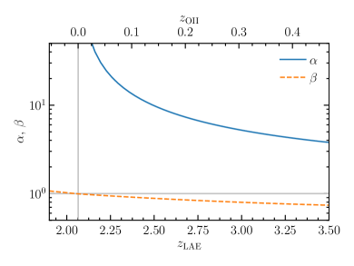
Figure 2: The scaling factors $\alpha$ (transverse) and $\beta$ (radial) as functions of redshifts ($z_{\mathrm{LAE}}$ on the lower axis and $z_{\mathrm{OII}}$ on the upper axis) for the fiducial $\Lambda$CDM model. The gray horizontal line marks no rescaling ($\alpha=\beta=1$), while the gray vertical line is the limit below which no interloping OIIEs exist.

3 Observed Correlation functions with interlopers

The presence of low-redshift interlopers in the high-redshift galaxy sample biases the clustering measurement. Similarly, the observed density contrast has extra contributions produced from the density contrast of the interlopers. In this section, we determine the effect interloping OIIEs have on the observed density contrast and two-point correlation functions of LAEs. First, we derive the effect on the observed density contrast and the two-point correlation function in configuration space, then Fourier-transform these quantities to derive the expression for the power spectrum.

Strictly speaking, one must fix the observed angular position and rescale only the radial position for each interloper. In this paper, however, we focus on the three-dimensional Fourier analysis by ignoring the opening-angle effect and by applying the scaling factors at the median redshift ($z_{\mathrm{LAE}}=2.7$ and $z_{\mathrm{OII}}=0.2$) to all interloping galaxies. This approach projects the interloping OIIEs from the true lower redshift cuboid volume to the high-redshift cuboid volume of LAEs. This approximation provides a good description for galaxy surveys with small sky coverage and a narrow range of redshifts, with the correction only proportional to the square of the opening angle, and the redshift bin size. It can be undoubtedly applied to galaxy surveys such as HETDEX ($\simeq$400\text{\,}\mathrm{d}\mathrm{e}\mathrm{g}\mathrm{{}^{2}}$$) and WFIRST ($\simeq$2000\text{\,}\mathrm{d}\mathrm{e}\mathrm{g}\mathrm{{}^{2}}$$). For galaxy surveys with broader sky coverage, we must employ different statistics based on the Fourier-Bessel or total angular momentum wave basis (Dai et al., 2012).

3.1 Observed density contrast with interlopers

Let us denote by $\bm{s}$ the position vector for the galaxies in the observed LAE sample and $\bm{s}^{\prime}$ the true position vector of the OIIE interlopers; i.e., $\bm{s}^{\prime}$ refers to the same angular position on the sky as $\bm{s}$, but with redshift $z_{\mathrm{OII}}$ instead of $z_{\mathrm{LAE}}$. Using the scaling factors in Eq. (7), $\bm{s}$ and $\bm{s}^{\prime}$ are related by

$$\bm{s}=(\alpha\bm{s}^{\prime}_{\perp},\beta s^{\prime}_{\parallel})\,,$$ (8)

where $\perp$ and $\parallel$ represent the components that are tangential and radial to the line of sight, respectively.

Note that Eq. (8) also holds for interlopers in redshift space, where the line-of-sight directional peculiar velocity $v_{\parallel}$ shifts the observed redshift $z_{\rm obs}$ away from the true redshift $z$ by $\left(1+z_{\rm obs}\right)=\left(1+z\right)\left(1+v_{\parallel}/c\right)$. As a result, the radial distance $r_{s}$ in redshift space is shifted relative to the real radial distance $r$ by $s=r+v_{\parallel}/aH$. The same scaling factor $\beta$, therefore, applies to both $r$ and $v_{\parallel}/aH$, when the observed redshift is misidentified.

With these position vectors and the variables defined in Eqs. (2)–(5), we can write the observed density contrast $\delta_{\mathrm{LAE}}^{\mathrm{obs}}(\bm{s})$ as a function of the true density contrast of LAEs $\delta_{\mathrm{LAE}}(\bm{s})$ and that of the OIIEs $\delta_{\mathrm{OII}}(\bm{s}^{\prime})$ as:

$$\delta_{\mathrm{LAE}}^{\mathrm{obs}}(\bm{s}) \equiv\frac{n^{\mathrm{obs}}_{\mathrm{LAE}}(\bm{s})}{\bar{n}^{\mathrm{obs}}_{\mathrm{LAE}}}-1$$

$$=(1-\mathfrak{f})\,\delta_{\mathrm{LAE}}(\bm{s})+\mathfrak{f}\,\delta_{\mathrm{OII}}(\bm{s}^{\prime})\,,$$ (9)

where mean number densities are defined in the LAE volume as $\bar{n}_{\mathrm{LAE}}\equiv N_{\mathrm{LAE}}/V_{\mathrm{survey}}$ and $\bar{n}_{\mathrm{OII}}\equiv N_{\mathrm{OII}}/V_{\mathrm{survey}}$, where $V_{\mathrm{survey}}$ is the LAE volume. Analogously, the observed OIIE density contrast is given by

$$\delta_{\mathrm{OII}}^{\mathrm{obs}}(\bm{s}^{\prime}) =\mathfrak{g}\,\delta_{\mathrm{LAE}}(\bm{s})+(1-\mathfrak{g})\,\delta_{\mathrm{OII}}(\bm{s}^{\prime})\,.$$ (10)

The observed density contrast is a superposition of the true LAE density contrast and the true OIIE density contrast, each contributing proportionally by number of galaxies in the sample.

Our analysis assumes that the true mean number densities ($\bar{n}_{\mathrm{LAE}}$, $\bar{n}_{\mathrm{OII}}$), and the misidentification fractions $x_{\mathrm{LAE}}$ and $x_{\mathrm{OII}}$, remain constant over the survey volume $V_{\mathrm{survey}}$. For realistic galaxy surveys, both the mean densities and the overall misidentification fractions may vary across the survey volume, which results in a nontrivial window function. We do not study the ramifications here, because the window function effect can be, in principle, modeled very accurately up to our knowledge of the survey conditions. For more discussion, see, for example, chapter 7 of Jeong (2010) and Chiang et al. (2013).

One subtle but important point is that we define the overall misidentification fractions $x_{\mathrm{LAE}}$ and $x_{\mathrm{OII}}$, as well as $\mathfrak{f}$ and $\mathfrak{g}$, in terms of the underlying, continuous galaxy number density fields $N_{\mathrm{LAE}}$ and $N_{\mathrm{OII}}$. In reality, the observed galaxy density fields are the distribution of discrete points (galaxies) that reflect these underlying continuous fields; therefore, locally measured values of $x_{\mathrm{LAE}}$ and $x_{\mathrm{OII}}$ are not necessarily the same across the survey volume. For instance, in an infinitesimal volume element we only expect a single LAE. Then, the misidentification fraction can be either unity (if the galaxy is an OIIE) or zero (if the galaxy is a genuine LAE). For the local quantities, therefore, the misidentification fractions $x_{\mathrm{LAE}}$ and $x_{\mathrm{OII}}$ are only statistical measures of the probability of misidentification.

Of course, the density contrasts given in Eqs. (9)–(10) must lead to the correct result for the galaxy two-point correlation function and power spectrum. The subtle difference appears in the treatment of shot noise. For example, for galaxies that are drawn randomly from a given continuous density field, the shot noise is proportional to the reciprocal of the total number density of galaxies, including the interlopers (shown in App. B).

3.2 Observed two-point correlation function with interlopers

The derivation in this section extends the Appendix A of Leung et al. (2017), including the two-point auto-correlation functions of both the main sample and the interloper sample. We calculate the observed two-point correlation function $\xi(\bm{s})=\big{<}\delta(\bm{r})\delta(\bm{r}+\bm{s})\big{>}$ in the configuration space from Eqs. (9)–(10) as

$$\xi_{\mathrm{LAE}}^{\mathrm{obs}}(\bm{s}) =\left<\delta_{\mathrm{LAE}}^{\mathrm{obs}}(\bm{r})\,\delta_{\mathrm{LAE}}^{\mathrm{obs}}(\bm{r}+\bm{s})\right>$$

$$=(1-\mathfrak{f})^{2}\,\xi_{\mathrm{LAE}}(\bm{s})+\mathfrak{f}^{2}\,\xi_{\mathrm{OII}}^{\mathrm{proj}}(\bm{s})$$

$$\quad+2(1-\mathfrak{f})\mathfrak{f}\,\xi_{\mathrm{LAE}\times{}\mathrm{OII}}(\bm{s})\,,$$ (11)

and

$$\xi_{\mathrm{OII}}^{\mathrm{obs}}(\bm{s}^{\prime}) =\left<\delta_{\mathrm{OII}}^{\mathrm{obs}}(\bm{r})\,\delta_{\mathrm{OII}}^{\mathrm{obs}}(\bm{r}+\bm{s}^{\prime})\right>$$

$$=(1-\mathfrak{g})^{2}\,\xi_{\mathrm{OII}}(\bm{s}^{\prime})+\mathfrak{g}^{2}\,\xi_{\mathrm{LAE}}^{\mathrm{proj}}(\bm{s}^{\prime})$$

$$\quad+2(1-\mathfrak{g})\mathfrak{g}\,\xi_{\mathrm{LAE}\times{}\mathrm{OII}}(\bm{s}^{\prime})\,.$$ (12)

Here,

$$\xi^{\text{proj}}_{\mathrm{OII}}(\bm{s}) =\xi_{\mathrm{OII}}(\bm{s}^{\prime})=\xi_{\mathrm{OII}}(\alpha^{-1}\bm{s}_{\perp},\beta^{-1}s_{\parallel})\,,$$ (13)

and

$$\xi^{\text{proj}}_{\mathrm{LAE}}(\bm{s}^{\prime}) =\xi_{\mathrm{LAE}}(\bm{s})=\xi_{\mathrm{LAE}}(\alpha\bm{s}_{\perp}^{\prime},\beta s_{\parallel}^{\prime})\,$$ (14)

are the OIIE and LAE two-point correlation functions projected to the wrongly assigned redshifts; therefore, they contaminate the two-point correlation function of the respective sample. Note that the projection merely relabels the coordinates (thus shifting the separation vector) while keeping intact the amplitude of the two-point correlation function.

The other terms in Eq. (11) and Eq. (12), $\xi_{\mathrm{LAE}\times\mathrm{OII}}$, denote the cross-correlation between the LAEs and projected OIIEs (evaluated at $\bm{s}$) and between the OIIEs and projected LAEs (evaluated at $\bm{s}^{\prime}$). They are much smaller than the respective auto-correlation functions because the wide radial separation between LAEs and OIIEs suppresses the true cross-correlation, and the cross-correlation from lensing is small. We can therefore ignore this contribution.

Our final expressions for the observed galaxy two-point correlation functions of LAEs and OIIEs are

$$\xi_{\mathrm{LAE}}^{\mathrm{obs}}(\bm{s}) =(1-\mathfrak{f})^{2}\,\xi_{\mathrm{LAE}}(\bm{s})+\mathfrak{f}^{2}\,\xi_{\mathrm{OII}}(\alpha^{-1}\bm{s}_{\perp},\beta^{-1}s_{\parallel})\,,$$ (15)

$$\xi_{\mathrm{OII}}^{\mathrm{obs}}(\bm{s}^{\prime}) =(1-\mathfrak{g})^{2}\,\xi_{\mathrm{OII}}(\bm{s}^{\prime})+\mathfrak{g}^{2}\,\xi_{\mathrm{LAE}}(\alpha\bm{s}_{\perp}^{\prime},\beta s_{\parallel}^{\prime})\,.$$ (16)

Eqs. (15)–(16) show that the different scaling factors ($\alpha\neq\beta$) introduce anisotropies into the two-point correlation functions. This is true even when $\xi(\bm{s})$ only depends on $s$ — for example, without the RSD.

3.3 Observed power spectrum with interlopers

We initially calculate the observed galaxy power spectrum by the Fourier transform of the corresponding two-point correlation function. The results of this section are consistent with those of Pullen et al. (2016) and Leung et al. (2017).

The Fourier transform integrates over the respective observed coordinates—$\bm{s}$ for LAEs and $\bm{s}^{\prime}$ for OIIEs—whose volume forms are related by the scaling parameters [Eq. (8)]

$$\mathrm{d}^{3}\!s =\mathrm{d}^{2}\!s_{\perp}\,\mathrm{d}s_{\parallel}=\alpha^{2}\beta\,\mathrm{d}^{3}\!s^{\prime}\,.$$ (17)

Using Eq. (15), we compute the observed LAE power spectrum as

$$P_{\mathrm{LAE}}^{\mathrm{obs}}({\bm{k}})=(1-\mathfrak{f})^{2}P_{\mathrm{LAE}}({\bm{k}})+\mathfrak{f}^{2}P_{\mathrm{OII}}^{\mathrm{proj}}({\bm{k}})\,,$$ (18)

where $P_{\mathrm{OII}}^{\mathrm{proj}}({\bm{k}})$ is the power spectrum of OIIEs (at $\bm{s}^{\prime}$) projected onto the LAE coordinates ($\bm{s}$), or the Fourier transform of Eq. (13):

$$P_{\mathrm{OII}}^{\mathrm{proj}}({\bm{k}}) \equiv\int\mathrm{d}^{3}\!s\,e^{i{\bm{k}}\cdot\bm{s}}\xi_{\mathrm{OII}}(\bm{s}_{\perp}^{\prime},s_{\parallel}^{\prime})$$

$$=\alpha^{2}\beta\int\mathrm{d}^{3}\!s^{\prime}e^{i(\alpha{\bm{k}}_{\perp}\cdot\bm{s}^{\prime}_{\perp}+\beta k_{\parallel}s^{\prime}_{\parallel})}\xi_{\mathrm{OII}}(\bm{s}_{\perp}^{\prime},s_{\parallel}^{\prime})$$

$$=\alpha^{2}\beta P_{\mathrm{OII}}(\alpha{\bm{k}}_{\perp},\beta k_{\parallel})\,.$$ (19)

Similarly, the power spectrum of the observed OIIEs is

$$P_{\mathrm{OII}}^{\mathrm{obs}}({\bm{k}})=(1-\mathfrak{g})^{2}P_{\mathrm{OII}}({\bm{k}})+\frac{\mathfrak{g}^{2}}{\alpha^{2}\beta}P_{\mathrm{LAE}}\left(\frac{{\bm{k}}_{\perp}}{\alpha},\frac{k_{\parallel}}{\beta}\right)\,.$$ (20)

Eq. (19) and Eq. (20) demonstrate how misinterpreting the emission-line redshifts leads to two effects. First, just as in the case for the two-point correlation functions, the misinterpretation shifts the scales, projecting small (large) scales onto larger (smaller) scales when OIIEs (LAEs) are misinterpreted as LAEs (OIIEs). This effect is illustrated in Fig. 1. Again, $\alpha\neq\beta$ introduces an additional anisotropy into the observed power spectrum beyond RSD. Second, the amplitude of the power spectrum is changed proportionally to the ratio between the true volume and the projected volume. For example, when OIIEs in a small, low-$z$ volume are projected into the larger, high-$z$ volume, the projected power spectrum amplitude is boosted by a factor of $\alpha^{2}\beta$.

3.4 The Observed Cross-correlation Functions

As discussed earlier, we ignore the true cross-correlation between the LAEs and OIIEs. Misidentification can, however, induce a cross-correlation between the OIIEs and LAEs because both observed samples contain high-$z$ and low-$z$ objects. Strictly speaking, such a cross-correlation must be measured in the angular cross-correlation function or in the angular cross-power spectrum. As we are adopting the flat-sky approximation throughout this paper, we mimic the angular cross-correlation by the three-dimensional cross-correlation between $\delta_{\mathrm{LAE}}^{\mathrm{obs}}(\bm{s})$ and $\delta_{\mathrm{OII}}^{\mathrm{obs}}(\alpha\bm{s}_{\perp},\beta\bm{s}_{\parallel})$ artificially placed at the corresponding LAE redshifts through Eq. (1). This procedure resembles the angular cross-correlation because for a given LAE redshift $z_{\mathrm{LAE}}$, the OIIE redshift $z_{\mathrm{OII}}$ is uniquely determined. Of course, one can also choose to correlate $\delta_{\mathrm{OII}}^{\mathrm{obs}}$ with $\delta_{\mathrm{LAE}}^{\mathrm{obs}}$ projected to the OIIE redshifts.

The cross-correlation function defined here is

$$\xi_{\mathrm{LAE}\times\mathrm{OII}}^{\mathrm{obs}}(\bm{s}) =\left<\delta_{\mathrm{LAE}}^{\mathrm{obs}}(\bm{r})\,\delta_{\mathrm{OII}}^{\mathrm{obs}}(\bm{r}+\bm{s})\right>$$

$$=(1-\mathfrak{f})\mathfrak{g}\xi_{\mathrm{LAE}}(\bm{s})+\mathfrak{f}(1-\mathfrak{g})\xi_{\mathrm{OII}}^{\mathrm{proj}}(\bm{s})\,,$$ (21)

with $\xi_{\mathrm{OII}}^{\mathrm{proj}}(\bm{s})$ given in Eq. (13), and the corresponding cross-power spectrum

$$P_{\mathrm{LAE}\times\mathrm{OII}}^{\mathrm{obs}}({\bm{k}})$$

$$=(1-\mathfrak{f})\mathfrak{g}P_{\mathrm{LAE}}({\bm{k}})+\mathfrak{f}(1-\mathfrak{g})\alpha^{2}\beta P_{\mathrm{OII}}(\alpha{\bm{k}}_{\perp},\beta k_{\parallel})\,.$$ (22)

The nonzero cross-correlation in Eq. (22) is the key for measuring the interloper fractions $\mathfrak{f}$ and $\mathfrak{g}$. This property is an effective indicator because we expect vanishingly small (contributions from the true clustering and the lensing magnification) cross-correlation for perfect ($\mathfrak{f}=\mathfrak{g}=0$) LAE and OIIE samples.

Similarly, we define the observed cross-correlation coefficient using the OIIE power spectrum projected into the LAE volume as

$$r \equiv\frac{P_{\mathrm{LAE}\times\mathrm{OII}}^{\mathrm{obs}}({\bm{k}})}{\sqrt{P_{\mathrm{LAE}}^{\mathrm{obs}}({\bm{k}})P_{\mathrm{OII}}^{\mathrm{obs},\mathrm{proj}}({\bm{k}})}}\,.$$ (23)

The value of $r$ varies continuously between $0$ and $1$ as a function of the interloper fractions $\mathfrak{f}$ and $\mathfrak{g}$. The cross-correlation coefficient $r$ reaches maximum ($r=1$) when $\mathfrak{f}+\mathfrak{g}=1$, and minimum ($r=0$) for the completely uncontaminated case ($\mathfrak{f}=\mathfrak{g}=0$) and the completely confused case ($\mathfrak{f}=\mathfrak{g}=1$) .

3.5 Modeling the Redshift-space Galaxy Power Spectrum

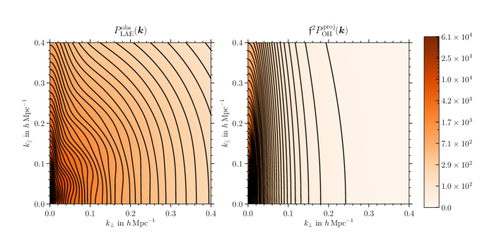
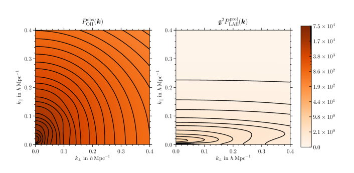
Figure 3: Left: the observed two-dimensional power spectra of LAEs (top, assuming $b_{\mathrm{LAE}}=2$ at $z_{\mathrm{LAE}}=2.7$) and OIIEs (bottom, assuming $b_{\mathrm{OII}}=1.5$ at $z_{\mathrm{OII}}=0.207$) including RSD, FoG, and the contributions from interlopers. We assume the interloper fraction of $\mathfrak{f}=\mathfrak{g}=0.1$. Right: contaminant power spectra from projected OIIEs (top) and LAEs (bottom) as they contribute to the observed power spectra in the left panels, i.e., the right panels contain an additional anisotropic feature, due to interlopers. The scaling factors are $\alpha=7.1$ and $\beta=0.84$.

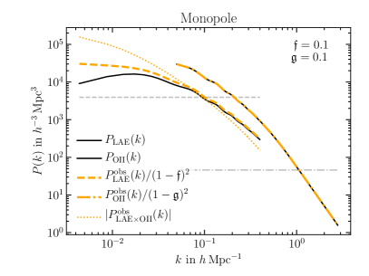
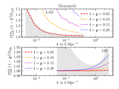
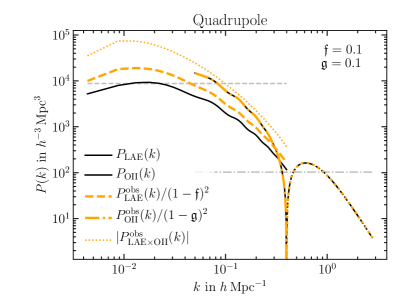
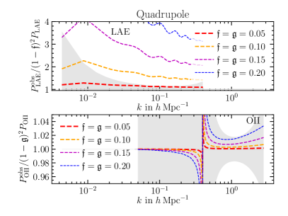
Figure 4: Top left: The solid black curves represent the fiducial LAE and OIIE monopole power spectra for the HETDEX survey. The orange dashed line indicates the observed LAE power spectrum with interloper fraction $\mathfrak{f}=0.1$; the orange dash-dotted line is the OIIE power spectrum with interloper fraction $\mathfrak{g}=0.1$. We rescale the amplitude of the observed power spectra so that they match the corresponding fiducial (black solid) power spectra when the contaminant contribution is negligible. The dotted orange lines show the monopole and quadrupole of the cross-power spectrum. The grey horizontal lines are the shot noise contribution $P_{\rm shot}^{\rm monopole}=1/\bar{n}_{g}$ and $P_{\rm shot}^{\rm quadrupole}=\sqrt{5}/{\bar{n}_{g}}$ with number density $\bar{n}_{g}$ (see App. C.3 for the general formula). For these values of the interloper fractions ($\mathfrak{f}=\mathfrak{g}=0.1$), the observed cross-correlation (orange dotted line) has a similar magnitude as the LAE power spectrum. Top right: The two panels in the top right panel compare the residual deviation of the observed LAE and OIIE power spectra shapes to the true power spectra for $\mathfrak{f},\mathfrak{g}=0.05,0.1,0.15,0.2$. The grey areas are the expected $1\sigma$ (68% C.L.) uncertainty ranges. Bottom right: The bottom panels show the same as the top panels, but for the quadrupole of the power spectrum. Here, the LAE redshift is $z_{\mathrm{LAE}}=2.7$ and the corresponding OIIE redshift is $z_{\mathrm{OII}}=0.207$.

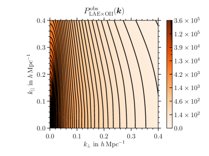
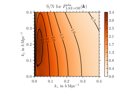
Figure 5: Left: The observed two-dimensional cross-power spectrum between LAEs and OIIEs (projected into LAE volume) with the interloper fractions $\mathfrak{f}=\mathfrak{g}=0.1$. In the case for HETDEX, the observed cross-correlation is dominated by the OIIE power spectrum, due to the large volume factor. Right: The bin-to-bin [$\Delta S=\left(\partial^{2}S/\partial k_{\perp}\partial k_{\parallel}\right)\Delta k_{\perp}\Delta k_{\parallel}$ with $\Delta k_{\perp}\Delta k_{\parallel}=k_{F}^{2}$] signal-to-noise (S/N) ratio for HETDEX with the interloper fractions $\mathfrak{f}=\mathfrak{g}=0.1$.

The expressions for the observed auto- and cross-power spectra of LAEs and OIIEs in terms of their true redshift-space power spectra are given in Eq. (18), Eq. (20), and Eq. (22). Thus, we can now complete the calculation with expressions for the true redshift-space power spectra of LAEs and OIIEs.

As a baseline model for the true redshift-space galaxy power spectrum, we adopt the linear bias model ($\delta_{g}(\bm{x})=b_{g}\delta_{m}(\bm{x})$, where $\delta_{g}(\bm{x})$ is the galaxy number density contrast, $b_{g}$ the linear galaxy bias parameter, and $\delta_{m}(\bm{x})$ the matter density contrast) with linear RSD (Kaiser, 1987) augmented by the Lorentzian Finger-of-God (FoG) damping (Jackson, 1972):

$$P_{x}({\bm{k}}) =\frac{(1+\beta_{x}\mu^{2})^{2}}{1+f^{2}(z_{x})k^{2}\mu^{2}\sigma_{v,x}^{2}}\,b_{x}^{2}D^{2}(z_{x})P_{\rm Lin}(k)\,.$$ (24)

Here, $D(z)$ is the linear growth factor, $f(z)$ is the linear growth rate ($f(z)\equiv\mathrm{d}\ln D/\mathrm{d}\ln a$), and $\beta_{x}\equiv f(z_{x})/b_{x}$, where we use the subscript $x=L$ for LAEs and $x=O$ for OIIEs. We define $\mu=\hat{{\bm{k}}}\cdot\hat{\bm{n}}=k_{\parallel}/k$ as the cosine of the angle between the wave vector and the line-of-sight direction. We model the FoG effect (Jackson, 1972) with a Lorentzian damping term via the one-dimensional velocity dispersion

$$\sigma_{v,x}^{2} =\frac{p}{3}\,D^{2}(z_{x})\int\frac{\mathrm{d}^{3}k}{(2\pi)^{3}}\,\frac{P_{\rm Lin}(k)}{k^{2}},$$ (25)

with a fudge parameter $p$. We adopt $p=0.4$, which Jeong (2010) measured from the two-dimensional redshift-space power spectrum of a suite of $N$-body simulations.

The left panels in Fig. 3 show the two-dimensional power spectra of LAEs (top) and OIIEs (bottom) in the $k_{\perp}$-$k_{\parallel}$ plane, with interloper fractions of $\mathfrak{f}=\mathfrak{g}=0.1$. Also displayed are the corresponding contamination from projected OIIEs ($P_{\mathrm{OII}}^{\mathrm{proj}}({\bm{k}})$) and LAEs ($P_{\mathrm{LAE}}^{\mathrm{proj}}({\bm{k}})$) in the right panels. Here, we use the linear bias of $b_{\mathrm{LAE}}=2$ and $b_{\mathrm{OII}}=1.5$ and assume that all LAEs are at $z=2.7$ while all OIIEs are at $z=0.2$, which yields the scaling factors $\alpha=7.1$ and $\beta=0.84$. These anisotropic scaling factors squeeze or stretch the power spectrum shapes. The effect is much larger along the perpendicular direction due to $\alpha\gg\beta\simeq 1$. To facilitate the comparison between the anisotropies from contamination and the total anisotropies in the observed power spectrum, we present the contribution from the interlopers in the right panels. For both LAEs and OIIEs, the small interloper fractions ($\mathfrak{f}$ and $\mathfrak{g}$) suppress the contribution from interlopers. The overall contribution, however, is much larger for the projected OIIEs (contaminating LAEs) because of the volume factor $\alpha^{2}\beta\simeq 40$; when projecting the high-redshift objects (such as LAEs) onto the lower redshift (to $z_{\mathrm{OII}}$), the power spectrum amplitude is suppressed by the factor $\alpha^{-2}\beta^{-1}$.

The angle-averaged, monopole power spectra are displayed in the top-left panel of Fig. 4. These spectra are shown without (black) and with (dashed orange) $\mathfrak{f}=\mathfrak{g}=$10\text{\,}\mathrm{\char 37\relax}$$ interloper fractions. For the contaminated spectra, we divide by a factor of $(1-\mathfrak{f})^{2}$ for LAEs and $(1-\mathfrak{g})^{2}$ for OIIEs to better compare the shape of the power spectra. The dotted line represents the observed cross-correlation, and the dashed (dash-dotted) grey horizontal lines indicate the shot noise for the LAEs (OIIEs). Note that the observed cross-correlation can exceed the LAE power spectrum.

To better demonstrate the effect of interlopers, the relative change of the monopole power spectrum is presented in the two top-right panels of Fig. 4; the very top panel for LAEs, the bottom for OIIEs. The grey areas indicate the fiducial error bars on the power spectrum that we discuss in Sec. 3.6. The colored dashed lines are the change for several contamination fractions as indicated in the legends. The most notable feature is that the LAE power spectrum is affected more strongly by interlopers than the OIIE power spectrum.

To investigate the angular dependence of the effect of interlopers, we present the quadrupole power spectrum in the bottom left panel of Fig. 4: the true quadrupoles (black lines), with $10\text{\,}\mathrm{\char 37\relax}$ interloper fractions (orange dashed for LAE, orange dash-dotted for OIIE), and the cross-correlation quadrupole (orange dotted). The graph reveals that, as for the monopole, the LAE power spectrum is more strongly affected by interlopers than the OIIE power spectrum.

The two bottom-right panels of Fig. 4 display the relative change of the power spectra for the quadrupole in the same manner as for the monopole. Again, the LAE quadrupole power spectrum is more strongly affected by contamination than the OIIE quadrupole.

Finally, the left panel of Fig. 5 shows the expected cross-correlation for $\mathfrak{f}=\mathfrak{g}=0.1$. The figure demonstrates that for a survey such as HETDEX, where the LAEs are at $z\sim 2.7$ and the OIIEs at $z\sim 0.2$, the contribution from the projected OIIE power spectrum is expected to dominate the observed cross-correlation.

3.5.1 On using the linear model of Eq. (24)

Strictly speaking, the linear theory prescription for the galaxy power spectrum [Eq. (24)] breaks down on small scales and we must include the nonlinear terms in our analysis. Indeed, for the HETDEX survey under consideration here, high-redshift ($1.9<z<3.5$) LAEs probe the quasi-linear scales $k\lesssim k_{\rm max}=$0.4\text{\,}\mathrm{\text{$h$}}\text{\,}{\mathrm{Mpc}}^{-1}$$, and corresponding lower-redshift OIIEs probe the fully-nonlinear scales to $k_{\rm max}\simeq$2\text{\,}\mathrm{\text{$h$}}\text{\,}{\mathrm{Mpc}}^{-1}$$ (the volume is smaller by a factor of $\left(\alpha^{2}\beta\right)^{-1}$, see Fig. 2). For the former, the complete next-to-leading order expression is given in Desjacques et al. (2018b) which includes nonlinearities in matter clustering, galaxy bias, and redshift-space distortion. For the fully-nonlinear regime, however, no such expression is known, and we may have to rely on cosmological simulations (Springel et al., 2018).

We therefore focus on analyzing the clustering of high-redshift LAEs rather than low-redshift OIIEs. We further assume that the interlopers do not dominate the high-redshift samples; this situation may be achieved by applying astrophysically-motivated classifications of emission lines (Pullen et al., 2016; Leung et al., 2017).

By focusing on the cosmological analysis from the LAE sample only, the model in Eq. (24) suffices to study the effect of interlopers on cosmological parameter estimation. As shown in Fig. 3 and Fig. 4, the misidentified low-$z$ interlopers (a) induce an anisotropy into the power spectrum and (b) increase large-scale power. The interlopers, therefore, affect the cosmological parameters measured from large scales $k<k_{\rm eq}$, where $k_{\rm eq}$ is the wavenumber corresponding to the matter-radiation equality (e.g., the local primordial non-Gaussianity parameter $f_{\mathrm{NL}}$), and from the anisotropies due to redshift-space distortion (e.g., the angular diameter distance $d_{A}(z)$, the Hubble expansion rate $H(z)$, and the linear growth rate $f(z)$). For the former, the linear theory applies because $k<k_{\rm eq}$ corresponds to sufficiently large scales. For the latter, the parameter estimation is relatively insensitive to the non-linearities such as the constraint on geometrical quantities from the BAO feature and Alcock-Paczynski (AP)-test (Alcock & Paczynski, 1979; Shoji et al., 2009). We explicitly check the effect of nonlinear redshift-space distortion in Sec. 4.7 by marginalizing the 2D power spectrum over higher powers in $\mu$.

3.6 Variance of the power spectrum measurement

Ignoring the connected trispectrum, we use only the Gaussian part of the covariance matrix where the power spectra at different wavevectors are statistically independent. We then calculate the variance (diagonal part of the covariance matrix) of the power spectrum as

$$\left(\Delta P({\bm{k}})\right)^{2} =\frac{2}{N_{{\bm{k}}}}\left(P({\bm{k}})+\frac{1}{{\bar{n}}_{g}}\right)^{2}$$ (26)

(see App. C for the derivation.) Here, $N_{{\bm{k}}}$ is the number of Fourier modes

$$N_{{\bm{k}}} =\frac{V_{\text{survey}}}{(2\pi)^{3}}\Delta V_{\bm{k}}\,,$$ (27)

with $\Delta V_{\bm{k}}$ being the volume in Fourier space contributing to the estimation of the power spectrum. For example, when computing the monopole power spectrum with the Fourier bin of $\Delta k=2\pi/V_{\mathrm{survey}}^{1/3}$,

$$\Delta V_{{\bm{k}}}=\Delta V(k,\Delta k)=4\pi k^{2}\Delta k\,.$$ (28)

When estimating the two-dimensional power spectrum $P(k_{\perp},k_{\parallel})$ with the Fourier bin of $(\Delta k_{\perp},\Delta k_{\parallel})$,

$$\Delta V_{{\bm{k}}}=\Delta V(k_{\perp},k_{\parallel},\Delta k_{\perp},\Delta k_{\parallel})=4\pi k_{\perp}\Delta k_{\perp}\Delta k_{\parallel}\,.$$ (29)

For the monopole matter power spectrum, Eq. (26) provides a good approximation to the measured variance from N-body simulations (Jeong & Komatsu, 2009).

The $1/{\bar{n}}_{g}$ term in Eq. (26) denotes the shot noise, assuming that the galaxy distribution follows the Poisson statistics of the underlying galaxy density field. When dealing with a galaxy sample containing the interlopers, the shot noise contribution to the observed auto-power spectrum is related to the number density $\bar{n}_{g}^{\rm total}$ of the total sample including the interlopers. Also, there is no shot noise contribution to the observed cross-power spectrum, even though both samples contain a mixture of the two populations. We present the rigorous derivation in App. B.

In App. C, we calculate the variance of the observed cross power spectrum as

$$\left(\Delta P_{LO}({\bm{k}})\right)^{2}$$

$$=\frac{1}{N_{\bm{k}}}\biggl{[}\left(P_{\mathrm{LAE}}^{\mathrm{obs}}({\bm{k}})+\frac{1}{\bar{n}_{\mathrm{LAE}}^{\rm total}}\right)\left(P_{\mathrm{OII}}^{\mathrm{obs},\mathrm{proj}}({\bm{k}})+\frac{\alpha^{2}\beta}{\bar{n}_{\mathrm{OII}}^{\rm total}}\right)$$

$$\quad+\big{(}P_{\mathrm{LAE}\times\mathrm{OII}}^{\mathrm{obs}}({\bm{k}})\big{)}^{2}\biggl{]}\,.$$ (30)

Here, $P_{\mathrm{OII}}^{\mathrm{obs},\mathrm{proj}}({\bm{k}})\equiv\alpha^{2}\beta P_{\mathrm{OII}}^{\mathrm{obs}}(\alpha{\bm{k}}_{\perp},\beta k_{\parallel})$ arises because we implement the cross-correlation by projecting the OIIEs onto the LAEs redshift (see Sec. 3.4). The same projection adds the factor $\alpha^{2}\beta$ to the shot noise of OIIEs. The right panel of Fig. 5 presents the signal-to-noise ratio for each $k_{\perp}$-$k_{\parallel}$ mode of the observed cross-power spectrum for the case $\mathfrak{f}=\mathfrak{g}=0.1$. This figure indicates that a high S/N ratio measurement for the interloper fraction is possible from the cross-correlation. We shall quantify this conclusion using a Fisher information matrix formalism in the next section.

4 Statistical Analysis for HETDEX

In this section, we present the statistical analysis for the cosmological parameter estimation from all three power spectra: the auto-power spectra of the main survey galaxies and the interlopers, and the cross-power spectrum between the main galaxies and interlopers.

In Sec. 4.1 we first construct the likelihood function for the dataset consisting of the main sample and the interlopers. We focus on the two geometrical observables measured from cosmological distortion: the Hubble expansion rate $H(z)$ and the angular diameter distance $d_{A}(z)$. These are primary targets for current and future galaxy surveys. We describe the cosmological distortion in the presence of the interloper population in Sec. 4.2. In Sec. 4.3, we present (Case A) the proof of concept for measuring the interloper fractions $\mathfrak{f}$ and $\mathfrak{g}$ from the cross-correlation between the main survey galaxies and interlopers. We measure the interloper fractions by assuming only that the true cross-correlation between the two populations vanishes.

In the following sub-sections, we present the projected uncertainties on $H(z)$ and $d_{A}(z)$ for several different treatments of nonlinearities in the redshift-space galaxy power spectrum. In Sec. (4.4)–(4.6), we assume that the redshift-space power spectrum is given by the linear Kaiser formula (Kaiser, 1987) with the Finger-of-God effect (Jackson, 1972) as in Eq. (24). In Sec. 4.4, we assume that we know the full shape of the nonlinear power spectrum $P(k)$ for both LAEs and OIIEs (Case B). Because OIIEs are lower redshift objects, their population probes much smaller scales than LAEs, and their nonlinearities are much stronger. We therefore investigate $H(z)$ and $d_{A}(z)$ after marginalizing over the nonlinear OIIE power spectrum in Sec. 4.5 (Case C), and we assume this case as a baseline for HETDEX. In Sec. 4.6, we study the pessimistic case of marginalizing over both LAE and OIIE power spectra (Case D). In this case, we can still measure the combination $d_{A}(z)H(z)$ given the Alcock-Paczynski test. In Sec. 4.7 we test for the effect of non-linear redshift-space distortion by including the higher-order dependence on the angular cosine $\mu\equiv k_{\parallel}/k$.

Finally, we analyze the effect of interlopers on measuring other cosmological parameters such as the linear growth rate $f=d\ln D/d\ln a$ (Sec. 4.4) and the primordial non-Gaussianity parameter $f_{\mathrm{NL}}$ (Sec. 4.8).

Throughout, we denote the true interloper fractions that we have assumed for the analysis by $\mathfrak{f}_{\mathrm{true}}$ and $\mathfrak{g}_{\mathrm{true}}$.

4.1 Likelihood function

We construct the likelihood function by assuming that the galaxy power spectrum completely specifies the statistics of the galaxy density contrast; i.e., we ignore the effects from higher-order correlation functions. Since we are focused on the galaxy power spectrum, this assumption suffices for the purpose of this paper.

To facilitate the calculation and to incorporate the auto- and cross-power spectra in the same setting, we project all OIIEs into the LAE volume. We could just as well have chosen to project all LAEs into the OIIE volume, or, similarly, project both LAEs and OIIEs into any appropriate volume of our choice. As seen from Eq. (4.1) below, the choice of projection merely adds a constant to the log-likelihood function.

The likelihood function is constructed from the observed density contrasts $\delta^{\mathrm{obs}}_{x}({\bm{k}}_{i})$, with $x=L$ for LAEs and $x=O$ for OIIEs, both of which are contaminated by interlopers. For each observed wavemode ${\bm{k}}$, we define the observed data vector at the LAE redshift (with OIIEs projected to that redshift) as

$$\Delta({\bm{k}}) =\begin{pmatrix}\Delta_{L}({\bm{k}})\\ \Delta_{O}^{\mathrm{proj}}({\bm{k}})\end{pmatrix}=\begin{pmatrix}\delta^{\mathrm{obs}}_{L}({\bm{k}}_{1})\\ \vdots\\ \delta^{\mathrm{obs}}_{L}({\bm{k}}_{N_{\bm{k}}})\\ \delta^{\mathrm{obs},\mathrm{proj}}_{O}({\bm{k}}_{1})\\ \vdots\\ \delta^{\mathrm{obs},\mathrm{proj}}_{O}({\bm{k}}_{N_{\bm{k}}})\\ \end{pmatrix}\,,$$ (31)

where $N_{\bm{k}}$ is the number of Fourier-modes for a given bin centered on ${\bm{k}}$. We provide the explicit expression for $N_{\bm{k}}$ in Eq. (27) and Eq. (29).

As shown in Sec. 3.6, each element of the covariance matrix consists of the observed power spectra plus Poisson shot noise $P_{xy}^{\mathrm{obs+shot}}({\bm{k}})=P^{\mathrm{obs}}_{xy}({\bm{k}})+\delta^{K}_{xy}/\bar{n}_{x}^{\mathrm{total}}$. Here, $\delta^{K}$ is the Kronecker delta symbol. In block-matrix form, the covariance matrix is

$$C({\bm{k}})=\langle\Delta({\bm{k}})\Delta^{\dagger}({\bm{k}})\rangle$$

$$=\frac{(2\pi)^{3}}{V_{\bm{k}}}\begin{pmatrix}P_{L}^{\mathrm{obs+shot}}({\bm{k}})I_{N_{\bm{k}}}&P_{LO}^{\mathrm{obs}}({\bm{k}})I_{N_{\bm{k}}}\\ P_{LO}^{\mathrm{obs}}({\bm{k}})I_{N_{\bm{k}}}&P_{O}^{\mathrm{obs+shot},\mathrm{proj}}({\bm{k}})I_{N_{\bm{k}}}\end{pmatrix}\,,$$ (32)

where $I_{N_{\bm{k}}}$ is the $N_{\bm{k}}\times N_{\bm{k}}$ unit matrix, and $P_{O}^{\mathrm{obs+shot},\mathrm{proj}}({\bm{k}})$ is the OIIE auto-power spectrum projected into the LAE volume. The factor $V_{\bm{k}}/(2\pi)^{3}$ appears from averaging $\langle\delta^{*}(\bm{q})\delta(\bm{q}^{\prime})\rangle=(2\pi)^{3}\delta^{D}(\bm{q}-\bm{q}^{\prime})P(\bm{q})$ over a cell of volume $V_{\bm{k}}$ in ${\bm{k}}$-space. From the covariance matrix, we compute the log-likelihood function

$$-\ln\mathfrak{L} =\frac{1}{2}\ln\det C+\frac{1}{2}\Delta^{\dagger}C^{-1}\Delta,$$ (33)

as

$$-\ln\mathfrak{L} =\sum_{\bm{k}}\frac{N_{\bm{k}}}{2}\bigg{[}\ln\big{[}P_{L}^{\mathrm{obs+shot}}P_{O}^{\mathrm{obs+shot},\mathrm{proj}}-(P_{LO}^{\mathrm{obs}})^{2}\big{]}$$

$$\quad+\frac{P_{O}^{\mathrm{obs+shot},\mathrm{proj}}\hat{P}_{L}^{\text{data+shot}}+P_{L}^{\mathrm{obs+shot}}\hat{P}_{O}^{\mathrm{data+shot},\mathrm{proj}}-2P_{LO}^{\mathrm{obs}}\hat{P}_{LO}^{\text{data}}}{P_{L}^{\mathrm{obs+shot}}P_{O}^{\mathrm{obs+shot},\mathrm{proj}}-(P_{LO}^{\mathrm{obs}})^{2}}\bigg{]}\,.$$ (34)

Here, we replace the square of the data vector with the maximum-likelihood estimators for the observed auto-power spectra:

$$\hat{P}_{L}^{\text{data+shot}}({\bm{k}}) =\frac{V_{\bm{k}}}{(2\pi)^{3}N_{\bm{k}}}\sum_{i}|\delta_{L}^{\mathrm{obs}}({\bm{k}}_{i})|^{2}\,,$$ (35)

$$\hat{P}_{O}^{\mathrm{data+shot,\mathrm{proj}}}({\bm{k}}) =\frac{V_{\bm{k}}}{(2\pi)^{3}N_{\bm{k}}}\sum_{i}|\delta_{O}^{\mathrm{obs},\mathrm{proj}}({\bm{k}}_{i})|^{2}\,,$$ (36)

and the cross-power spectrum

$$\hat{P}_{LO}^{\text{data}}({\bm{k}}) =\frac{V_{\bm{k}}}{(2\pi)^{3}N_{\bm{k}}}\sum_{i}\Re\big{(}\delta_{L}^{\mathrm{obs},*}({\bm{k}}_{i})\delta_{O}^{\mathrm{obs},\mathrm{proj}}({\bm{k}}_{i})\big{)}\,,$$ (37)

where $\Re(z)$ is the real part of a complex number $z$.

4.2 Cosmological distortion

Cosmological distortion refers to the systematic change in the statistical observables, such as the galaxy power spectrum, induced by adopting an incorrect reference cosmology to convert the observed galaxy coordinate (RA, Dec, $z$) into physical coordinates. Cosmological distortion allows us to measure the Hubble expansion rate $H(z)$ and the angular diameter distance $d_{A}(z)$ from features such as those produced by BAO (Seo & Eisenstein, 2003; Blake & Glazebrook, 2003; Hu & Haiman, 2003) and the AP-test (Alcock & Paczynski, 1979; Shoji et al., 2009) in the redshift-space galaxy power spectrum. In this paper, we do not include the uncertainties in the cosmological parameters such as $\Omega_{\rm m}h^{2}$ and $\Omega_{\rm b}h^{2}$ that determine the shape of the linear matter power spectrum. In the real analysis, one must include appropriate priors on these parameters from, e.g., the CMB analysis in, e.g., (Planck Collaboration, 2016b; Planck Collaboration et al., 2018).

We model the cosmological distortion in the galaxy power spectrum as follows. Given a reference cosmology, we calculate the angular diameter distance $d_{A,\text{ref}}(z)$ as well as the Hubble expansion rate $H_{\text{ref}}(z)$ at redshift $z$. In general, the wavenumbers $k_{\perp}^{\text{ref}}$ and $k_{\parallel}^{\text{ref}}$ measured from the reference cosmology differ from the true wavenumbers $k_{\perp}$ and $k_{\parallel}$ by some factors $v(z)$ and $w(z)$. We determine the factors $v(z)$ and $w(z)$ and their effect on the power spectrum in a manner similar to the projection effect discussed in Sec. 3 using $\alpha$ and $\beta$. For LAEs (subscript ‘L’) and OIIEs (subscript ‘O’), we define

$$v_{L} =\frac{d_{A,\text{ref}}(z_{L})}{d_{A}(z_{L})}\,, w_{L} =\frac{H(z_{L})}{H_{\text{ref}}(z_{L})}\,,$$ (38)

$$v_{O} =\frac{d_{A,\text{ref}}(z_{O})}{d_{A}(z_{O})}\,, w_{O} =\frac{H(z_{O})}{H_{\text{ref}}(z_{O})}\,.$$ (39)

Using these variables, the Fourier space vector $(k_{\perp}^{\text{ref}},k_{\parallel}^{\text{ref}})$ inferred from the reference cosmology is related to the true Fourier vector as $(k_{\perp},k_{\parallel})=(v_{L}k_{\perp}^{\text{ref}},w_{L}k_{\parallel}^{\text{ref}})$, and the power spectrum $P_{L}^{\text{ref}}(k^{\text{ref}}_{\perp},k_{\parallel}^{\rm ref})$, measured by using the reference cosmology, is

$$P_{L}^{\text{ref}}(k_{\perp}^{\text{ref}},k_{\parallel}^{\text{ref}}) =v_{L}^{2}w_{L}P_{L}(v_{L}k_{\perp}^{\text{ref}},w_{L}k_{\parallel}^{\text{ref}})\,.$$ (40)

Similarly, we calculate the contribution from the projected interloper power spectrum by defining $\alpha_{\text{ref}}$ and $\beta_{\text{ref}}$ as the scaling factors $\alpha$ and $\beta$ [Eq. (7)] in the reference cosmology. The projected OIIE power spectrum takes the following form, where we include both the projection due to the misidentification [see Eq. (19)], and the projection due to a cosmological distortion [Eq. (4.2)]:

$$P_{O}^{\text{ref,proj}}(k_{\perp}^{\text{ref}},k_{\parallel}^{\text{ref}})$$

$$=\alpha_{\text{ref}}^{2}\beta_{\text{ref}}P_{O}^{\text{ref}}(\alpha_{\text{ref}}k_{\perp}^{\text{ref}},\beta_{\text{ref}}k_{\parallel}^{\text{ref}})$$

$$=\alpha_{\text{ref}}^{2}\beta_{\text{ref}}v_{O}^{2}w_{O}P_{O}(v_{O}\alpha_{\text{ref}}k_{\perp}^{\text{ref}},w_{O}\beta_{\text{ref}}k_{\parallel}^{\text{ref}})\,.$$ (41)

The parameters $\alpha_{\rm ref}$ and $\beta_{\rm ref}$ are completely degenerate with $v_{L}$, $v_{O}$ and $w_{L}$, $w_{O}$; therefore, we only include the latter cosmological distortion parameters in the analysis.

4.3 Case A: No prior knowledge on the shape of the galaxy power spectra

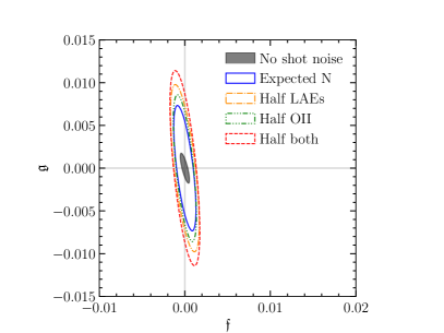
Figure 6: Constraints on the interloper fractions $\mathfrak{f}$ and $\mathfrak{g}$ for HETDEX. The shaded ellipse represents the $1\sigma$ ($68\text{\,}\mathrm{\char 37\relax}$ C.L.) interval when there is no shot noise. The blue solid ellipse is the $1\sigma$ (68% C.L.) interval for the expected numbers of LAEs and OIIEs, the orange dash-dotted is the same $1\sigma$ interval for when the number of LAEs is halved, the green line with several dots between dashes is the result when the OIIE number is halved, and the red dashed line indicates what occurs when both numbers are halved. Here, $\mathfrak{f}_{\mathrm{true}}=\mathfrak{g}_{\mathrm{true}}=0$.

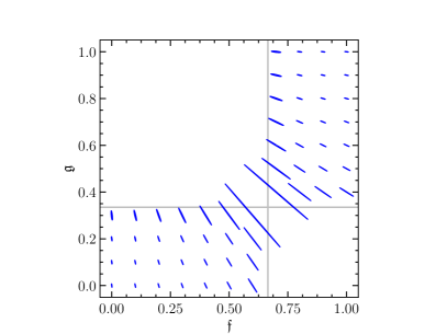
Figure 7: Constraints on the interloper fractions $\mathfrak{f}$ and $\mathfrak{g}$ for several interloper fractions spaced $10\text{\,}\mathrm{\char 37\relax}$ apart. Since $N_{\mathrm{OII}}^{\mathrm{true}}/N_{\mathrm{LAE}}^{\mathrm{true}}\approx 2$ for HETDEX, only the interloper fractions bounded by the grey lines are physically possible (see App. A). However, since the true number densities will not be known, and thus cannot be used in the fit, estimates of $\mathfrak{f}$ and $\mathfrak{g}$ may well fall outside those boundaries. $\mathfrak{f}$ and $\mathfrak{g}$ can be measured best near $(0,0)$ and $(1,1)$. On the diagonal $\mathfrak{f}+\mathfrak{g}=1$, the individual measurements become degenerate.

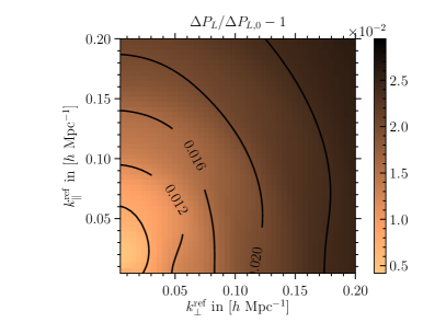
Figure 8: Change in the uncertainty of the power spectrum relative to the ideal case of zero interloper fractions, i.e., $[\Delta P_{L}({\bm{k}})/\Delta P_{L,0}({\bm{k}})]-1$, where we marginalize over $\mathfrak{f}$, $\mathfrak{g}$, and $P_{O}({\bm{k}})$. To first order, the increase in uncertainty is the least where the product $\bar{n}P$ is largest. Here, $\mathfrak{f}_{\mathrm{true}}=\mathfrak{g}_{\mathrm{true}}=0.01$.

How accurately can we measure the interloper fractions $\mathfrak{f}$ and $\mathfrak{g}$ by requiring only that the true cross-power spectrum must vanish? We address this question in the most conservative manner, assuming no prior knowledge about the shape of the galaxy power spectrum; i.e., the case where we measure the interloper fractions $\mathfrak{f}$ and $\mathfrak{g}$ along with the amplitude of the two-dimensional power spectrum $P_{L}(k_{\perp},k_{\parallel})$ and $P_{O}(k_{\perp},k_{\parallel})$ from fitting the observed auto- and cross-power spectra. The expressions for these power spectra are given in Eq. (18) and Eq. (20) (for the auto-power spectra) and Eq. (22) (for the cross-power spectrum).

For the HETDEX survey outlined in Sec. 2.1, there are $91^{2}=8281$ Fourier modes within the maximum wavenumber $k_{\rm max}=0.4~{}h/{\rm Mpc}$ at the LAE volume. Thus, there are a total of $2~{}(\mathfrak{f}~{}{\rm and}~{}\mathfrak{g})+8281~{}({\rm for}~{}P_{L})+8281~{}({\rm for}~{}P_{O})=16564$ parameters. For each value of $\mathfrak{f}$ and $\mathfrak{g}$, we use the Fisher information matrix analysis to calculate the projected uncertainties.

A cautionary remark is in order here. The analysis in this section only serves as a proof of concept for the measurement of the interloper fractions $\mathfrak{f}$ and $\mathfrak{g}$. The uncertainties found here are a worst case benchmark, because they are derived from minimal assumptions about the shape of the galaxy power spectrum. However, we do not advocate such an analysis in practice. In fact, we carried out a Markov-chain Monte Carlo (MCMC) analysis for the HETDEX case only to find that the chain does not converge in the 16564-dimensional parameter space. Even for a simpler analysis of measuring $\mathfrak{f}$ and $\mathfrak{g}$ by iteration, it is non-trivial to construct an unbiased estimator.

Fig. 6 presents the projected uncertainties on $\mathfrak{f}$ and $\mathfrak{g}$ under the null hypothesis, i.e., when the true interloper fractions are zero. The shaded ellipse at the center indicates the cosmic-variance limited constraint without shot noise. The solid ellipse shows the constraint with the fiducial number density of HETDEX given in Sec. 2.1. The forecast demonstrates that the cross-correlation constrains both $\mathfrak{f}$ and $\mathfrak{g}$ to the sub-percent level. The constraint is better for $\mathfrak{f}$ than $\mathfrak{g}$ because on large-scales where the signal-to-noise ratio is the largest (Fig. 5) the amplitude of the projected OIIE power spectrum (the contaminant) is much higher than that for the LAEs; this behavior is clear in the upper two panels in Fig. 3. In the Figure, the relative contributions of $P_{\mathrm{LAE}}$ and $P_{\mathrm{OII}}^{\mathrm{proj}}$ to the observed auto-correlation are similar on large-scales even though the latter is suppressed by $\mathfrak{f}^{2}$.

We also investigate the effect of reducing the number density of LAEs and OIIEs. The orange dash-dotted ellipse, the green triple-dot-dashed line, and the red dashed line show the expected constraint when reducing the number of LAEs, OIIEs, or both galaxy groups, respectively, by $50\text{\,}\mathrm{\char 37\relax}$ of what is predicted. Reducing the number density of galaxies increases the Poisson shot noise which affects the uncertainties in the power spectrum measurements on small scales. This change affects the constraint on $\mathfrak{g}$ more than $\mathfrak{f}$, due to the different scale-dependence of the $\mathfrak{f}$ and $\mathfrak{g}$ contributions. Fig. 3 reflected this behavior in the top- and bottom-right panels.

We next address the situation of non-zero $\mathfrak{f}$ and $\mathfrak{g}$. As shown in App. A, unlike the misidentification fractions $x_{\mathrm{LAE}}$ and $x_{\mathrm{OII}}$ [defined in Eqs. (2)–(3)] that can take any value between 0 and 1, the true interloper fractions are limited to two regions: one with $0\leq\mathfrak{f}_{\mathrm{true}}\leq\mathfrak{f}_{\mathrm{lim}}$ and $0\leq\mathfrak{g}_{\mathrm{true}}\leq\mathfrak{g}_{\mathrm{lim}}$, and one with $\mathfrak{f}_{\mathrm{lim}}\leq\mathfrak{f}_{\mathrm{true}}\leq 1$ and $\mathfrak{g}_{\mathrm{lim}}\leq\mathfrak{g}_{\mathrm{true}}\leq 1$. The limiting values $\mathfrak{f}_{\rm lim}=N_{\mathrm{OII}}^{\mathrm{true}}/(N_{\mathrm{LAE}}^{\mathrm{true}}+N_{\mathrm{OII}}^{\mathrm{true}})$ and $\mathfrak{g}_{\rm lim}=N_{\mathrm{LAE}}^{\mathrm{true}}/(N_{\mathrm{LAE}}^{\mathrm{true}}+N_{\mathrm{OII}}^{\mathrm{true}})$ occur when $x_{\mathrm{LAE}}+x_{\mathrm{OII}}=1$. For HETDEX, $\mathfrak{f}_{\mathrm{lim}}\approx 2/3$ and $\mathfrak{g}_{\mathrm{lim}}\approx 1/3$.

Fig. 7 presents the projected $68\text{\,}\mathrm{\char 37\relax}$ confidence ellipses of $\mathfrak{f}$ and $\mathfrak{g}$ for several true interloper fractions spread throughout the allowed region at intervals of $10\text{\,}\mathrm{\char 37\relax}$. The tightest constraints are obtained when the interloper fractions are either small or extremely large. There is a symmetry of exchanging $\mathfrak{f}\leftrightarrow 1-\mathfrak{g}$, which is equivalent to swapping the two samples. Indeed, a closer inspection of the log-likelihood given in Eq. (4.1) reveals that the cross-correlation alone cannot distinguish which of the two regions a given survey will fall into. However, since we expect the power spectra of LAEs and OIIEs to have very different shapes on large scales, inspection of the measured true power spectra should suffice to discriminate the two regions in cases far from the diagonal $\mathfrak{f}+\mathfrak{g}=1$. Because all three observed power spectra are the same, $\mathfrak{f}$ and $\mathfrak{g}$ are completely degenerate on the diagonal $\mathfrak{f}+\mathfrak{g}=1$. In that case, although the non-zero cross-correlation indicates the existence of interlopers, Eq. (18) and Eq. (20) cannot be inverted. The cross-correlation alone, therefore, is insufficient to determine the interloper fraction; this is the reason why the error ellipse diverges at $(\mathfrak{f}_{\rm lim},\mathfrak{g}_{\rm lim})$.

Although we plot the projected constraints on $\mathfrak{f}$ and $\mathfrak{g}$ only in the limited regions, an analysis with measured data must explore the whole range of $\mathfrak{f}$ and $\mathfrak{g}$ between $0$ and $1$. This is because the limits $\mathfrak{f}_{\rm lim}$ and $\mathfrak{g}_{\rm lim}$ are given by the true ratio $N_{\mathrm{LAE}}^{\mathrm{true}}/N_{\mathrm{OII}}^{\mathrm{true}}$, and in reality only the observed numbers of galaxies will be known; the true number of LAEs and OIIEs will be variables that need to be estimated from the observed numbers and the estimated interloper fractions. Thus, while the true interloper fractions are restricted to the allowed regions, the measured interloper fractions $\mathfrak{f}$ and $\mathfrak{g}$ can have any value between $0$ and $1$.

How do the uncertainties in measuring the power spectrum change due to the interlopers? Fig. 8 displays the change in the uncertainty on each mode $P_{L}(k_{\perp},k_{\parallel})$ after marginalizing over the interloper fractions. Here, we use $\mathfrak{f}_{\mathrm{true}}=\mathfrak{g}_{\mathrm{true}}=0.01$. Fig. 8 shows that the fractional increase in the uncertainties in the power spectrum closely follows $\bar{n}P$: the power spectrum uncertainties increase mainly in the shot noise dominated regime ($\bar{n}_{L}P_{L}\ll 1$) and the increase only depends on the interloper fractions and the number of galaxies.

We can estimate the increase in the uncertainty by inverting Eq. (18) and Eq. (20) for fixed $\mathfrak{f}$ and $\mathfrak{g}$, which is valid when $\mathfrak{f}$ and $\mathfrak{g}$ are tightly constrained (which is the case for small values, see Fig. 7). Combining this result with Eq. (26), to first order in $\mathfrak{f}$ and $\mathfrak{g}$, we obtain the uncertainty $\Delta P_{L}$ in the LAE power spectrum

$$\Delta P_{L}({\bm{k}}) \simeq\sqrt{\frac{2}{N_{\bm{k}}}}\left[P_{L}({\bm{k}})+\left(1+\mathfrak{f}+\mathfrak{g}\,\frac{\bar{n}_{O}}{\bar{n}_{L}}\right)\frac{1}{\bar{n}_{L}}\right]\,,$$ (42)

which is the same as Eq. (26), except that the shot-noise term is increased due to the interlopers. The fractional increase of the uncertainty is

$$\frac{\Delta P_{L}({\bm{k}})}{\Delta P_{L,0}({\bm{k}})}-1 \simeq\left(\frac{\mathfrak{f}\,\bar{n}_{L}+\mathfrak{g}\,\bar{n}_{O}}{\bar{n}_{L}}\right)\frac{1}{1+\bar{n}_{L}P_{L}^{\mathrm{ref}}({\bm{k}}_{\mathrm{ref}})}\,,$$ (43)

where $\Delta P_{L,0}$ is the uncertainty without interlopers. Eq. (43) is consistent with the results seen in Fig. 8. The estimate in Eq. (43) reproduces the numerical result to $\sim 3\text{\,}\mathrm{\char 37\relax}$ for $\mathfrak{f}_{\mathrm{true}}=\mathfrak{g}_{\mathrm{true}}=0.01$ and to $\sim 30\text{\,}\mathrm{\char 37\relax}$ for $\mathfrak{f}_{\mathrm{true}}=\mathfrak{g}_{\mathrm{true}}=0.1$. This difference is because, for larger values of $\mathfrak{f}_{\mathrm{true}}$ and $\mathfrak{g}_{\mathrm{true}}$, the linear expansion is not accurate and the larger uncertainties in $\mathfrak{f}$ and $\mathfrak{g}$ also contribute to $\Delta P_{L}$.

4.4 Case B: knowing full shape of both LAE and OIIE power spectrum

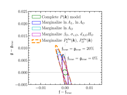
Figure 9: $1\sigma$ (68% C.L.) ellipses on interloper fractions $\mathfrak{f}$ and $\mathfrak{g}$ for several models. The first four models correspond to Case B, where we assume that the shapes of the power spectra are fully known. For the first model in green only the interloper fractions are being fit, all other parameters including the amplitudes are assumed to be known a priori. For the second, in blue, we marginalize over the amplitudes. For the third (solid cyan), we marginalize over the OIIE amplitude only, and for the fourth (solid magenta) over the RSD, FOG, and AP parameters of the OIIEs. Finally, the thick dashed orange ellipses correspond to the worst-case scenario, Case A, where only the cross-correlation is known, marginalizing over both 2D-power spectra. We consider two interloper fractions: $\mathfrak{f}_{\mathrm{true}}=\mathfrak{g}_{\mathrm{true}}=0$ and $\mathfrak{f}_{\mathrm{true}}=\mathfrak{g}_{\mathrm{true}}=0.2$, as labeled in the figure. Most of the measurement uncertainty on $\mathfrak{f}$ and $\mathfrak{g}$ is a result of marginalizing over the amplitudes.

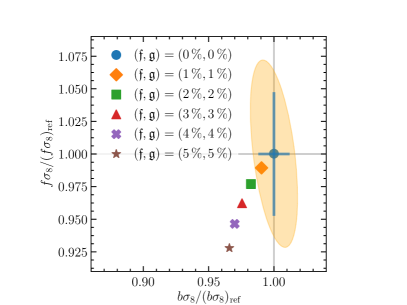
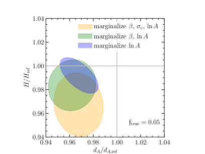
Figure 10: Left: The interloper bias for $f\sigma_{8}$ and $b\sigma_{8}$, for uncorrected interloper fractions $\mathfrak{f}=0,1,2,3,4,$5\text{\,}\mathrm{\char 37\relax}$$. The grey lines show the fiducial value, the ellipse gives the $1\sigma$ ($68\text{\,}\mathrm{\char 37\relax}$ C.L.) uncertainty, and the cross shows the marginalized uncertainties. Right: The interloper bias on distances ($d_{A}$ and $H$) when ignoring the interloper fraction $\mathfrak{f}=$5\text{\,}\mathrm{\char 37\relax}$$. The grey lines indicate the fiducial value. The bias tends to be more severe when marginalizing over more parameters.

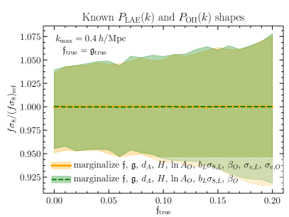
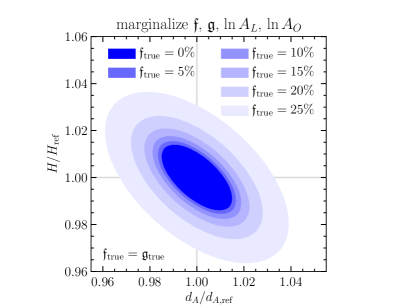
Figure 11: Left: Results from the joint-analysis method: $1\sigma$ ($68\text{\,}\mathrm{\char 37\relax}$ C.L.) limits on $f\sigma_{8}$ when the shape of both the LAE and OIIE power spectra are known, corresponding to Case B. The measurement is unbiased for both sets of marginalizations. Right: Results from the joint-analysis method: $1\sigma$-confidence ellipses on the angular diameter distance $d_{A}$ and the Hubble expansion rate $H$ at $z_{\mathrm{LAE}}=2.7$. The ellipses represent several values of the interloper fractions $\mathfrak{f}_{\mathrm{true}}$ and $\mathfrak{g}_{\mathrm{true}}$ as shown in the legend. The grey lines indicate the fiducial $d_{A}$ and $H$ values. Here, we marginalize over the interloper fractions and the amplitudes of the power spectra. Larger interloper fractions lead to larger errors.

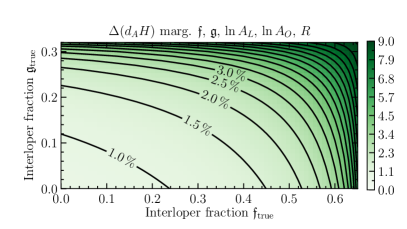
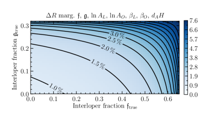
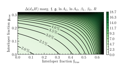
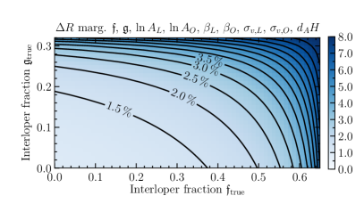
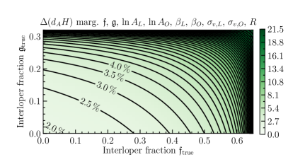
Figure 12: Results from the joint-analysis method: the change of $1\sigma$ (68% C.L.) uncertainties on $R=(d_{A}^{2}/H)^{1/3}$ (left) and $d_{A}H$ (right) as a function of true interloper fractions $(\mathfrak{f}_{\mathrm{true}},\mathfrak{g}_{\mathrm{true}})$ for Case B, when the shapes of the LAE and OIIE power spectra are both known. For each point in each panel, we set the true interloper fractions as given by the axes and we marginalize over the measured interloper fractions and the power spectrum amplitudes. We consider three models, from top to bottom: 1) assume the redshift space distortion parameters are known, 2) marginalize over $\beta_{x}=f(z_{x})/b_{x}$, and 3) additionally marginalize over the FoG velocity dispersion $\sigma_{v,x}$. With our method the forecast constraints on $R$ remain $\lesssim$1.5\text{\,}\mathrm{\char 37\relax}$$ up to interloper fractions $\sim 20\text{\,}\mathrm{\char 37\relax}$. The best constraints on $R$ are at the origin; from top to bottom, $0.88\text{\,}\mathrm{\char 37\relax}$, $0.9\text{\,}\mathrm{\char 37\relax}$, and $1.02\text{\,}\mathrm{\char 37\relax}$. The best constraints on $d_{A}H$ at the origin are $0.79\text{\,}\mathrm{\char 37\relax}$, $1.82\text{\,}\mathrm{\char 37\relax}$, and $1.92\text{\,}\mathrm{\char 37\relax}$, respectively.

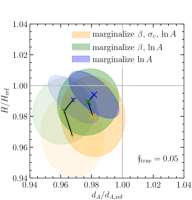
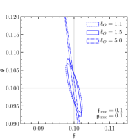
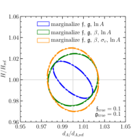
Figure 13: Dependence of various parameters on the amplitude of the OIIE power spectrum, parametrized by $b_{O}$. Left: The darker ellipses show the effect of the interloper bias on $d_{A}$ and $H$ assuming an OIIE linear galaxy bias $b_{O}=1.1$; the lighter ones are as in Fig. 10 for $b_{O}=1.5$. If $b_{O}=5$, the bias on $d_{A}H$ is $\sim 2030\text{\,}\mathrm{\char 37\relax}$, and $\sim 1035\text{\,}\mathrm{\char 37\relax}$ on $H$. The symbols mark the centers of the ellipses. Here we use $\mathfrak{f}_{\mathrm{true}}=\mathfrak{g}_{\mathrm{true}}=$5\text{\,}\mathrm{\char 37\relax}$$. Center: Constraints on interloper fractions $\mathfrak{f}$ and $\mathfrak{g}$ for $\mathfrak{f}_{\mathrm{true}}=\mathfrak{g}_{\mathrm{true}}=$10\text{\,}\mathrm{\char 37\relax}$$ for Case B. Dashed lines use a bias of $b_{O}=1.1$, solid lines assume $b_{O}=1.5$ (our fiducial value throughout the rest of the paper), and dashed-dotted use $b_{O}=5$. A larger OIIE bias reduces the uncertainty on $\mathfrak{f}$ and increases the uncertainty on $\mathfrak{g}$. Right: The constraints on $d_{A}$ and $H$, marginalizing over parameters as indicated in the legend. The figure demonstrates that the OIIE bias does not affect the uncertainty on $d_{A}$ and $H$, since for each of the three marginalizations considered, the three $b_{O}$ ellipses lie on top of each other.

We now address the case of the opposite limit where one can model the full shape of the galaxy power spectrum for both LAEs and OIIEs using Eq. (24). This is perhaps an unrealistically optimistic case, but it does allow us to set another benchmark point for the effect of interlopers on the measurement of cosmological parameters such as the angular diameter distance and the Hubble expansion rate. The list of parameters that we include in the analysis is: the interloper fractions $\mathfrak{f}$ and $\mathfrak{g}$, and for each type of tracer the power spectrum amplitude $\ln A$, the angular diameter distance $d_{A}$, the Hubble expansion rate $H$, the redshift space distortion parameter $\beta=f/b_{1}$, and the velocity dispersion $\sigma_{v}^{2}$, for a total of up to 12 parameters.

First, we study the projected uncertainties in measuring $\mathfrak{f}$ and $\mathfrak{g}$. Fig. 9 shows the Fisher forecasts for several cases from maximal a priori knowledge where we assume we have complete knowledge of the power spectra and only the interloper fractions are being fitted, to minimal a priori knowledge, where only the true cross-correlation is known beforehand, i.e. our Case A. For each case Fig. 9 displays the $68\text{\,}\mathrm{\char 37\relax}$ C.L. ($1\sigma$) contours for two values: $\mathfrak{f}_{\mathrm{true}}=\mathfrak{g}_{\mathrm{true}}=0$ (inner ellipses) and $0.2$ (outer ellipses).

Of course, assuming the complete knowledge on the shape of the galaxy power spectrum enhances the constraint on the contamination fractions. Between the optimistic case (green, central ellipses) and the pessimistic case (thick, outer-most ellipses) are three cases in which we marginalize over different combinations of parameters. Intriguingly, marginalizing over the full 2D power spectra and marginalizing over just the amplitudes of the power spectra gives rise to similar constraints on the interloper fractions. Indeed, for $\mathfrak{f}=\mathfrak{g}=0$, there is no change between the two, and only at interloper fractions $\mathfrak{f}=\mathfrak{g}=20\%$ is the difference apparent. Marginalizing over the parameters controlling the shape of the redshift-space power spectrum of OIIEs ($\beta_{O}$, $\sigma_{v,O}$ and $d_{A,O}H_{O}$) also changes the $\mathfrak{f}$ and $\mathfrak{g}$ constraints significantly. The effects of marginalizing over other parameters are not as dramatic.

Pullen et al. (2016) demonstrated that ignoring interlopers in the galaxy sample biases the estimation of cosmological parameters, such as the linear growth rate $f$ and the galaxy bias $b_{g}$. Similarly, the left panel of Fig. 10 presents the bias on $f\sigma_{8}$ and $b\sigma_{8}$ induced by ignoring the interlopers, and the right panel of Fig. 10 shows that this interloper bias also plagues the distance measurement. We simulate the interloper bias by generating a realization of the LAE power spectrum with $\mathfrak{f}_{\mathrm{true}}=$5\text{\,}\mathrm{\char 37\relax}$$ but ignore the contamination by fixing $\mathfrak{f}=0$ in the analysis. For the analysis, we use an MCMC algorithm with the adaptive Metropolis sampler (Roberts & Rosenthal, 2009), and find the interloper bias by running MCMC on the ensemble-averaged log-likelihood function. We also check that the result is consistent with the first-order analytical calculation presented in App. D. In the appendix we also justify the use of the ensemble-averaged log-likelihood.

For each set of parameters (as indicated at the beginning of this section and the figures), we ran the chain with $$1000$\,N_{p}(N_{p}+1)$ iterations, where $N_{p}$ is the number of parameters, updating the covariance matrix of the proposal distribution every $N_{p}(N_{p}+1)$ steps with $\beta=0.95$ (see Eq.(2.1) in Roberts & Rosenthal, 2009). The first half of the iterations are discarded to allow the proposal distribution to settle, and the analysis is performed on the second half. We use a flat prior as long as the parameters are within physical limits. The exceptions are that the auto-power spectra are additionally limited to $\leq{10}^{6}\text{\,}{\mathrm{\text{$h$}}}^{-3}\text{\,}{\mathrm{Mpc}}^{3}$, and in later sections (Case C and Case D) the cosmological distortion parameters $v_{L}$, $w_{L}$, $v_{O}$, and $w_{O}$ are additionally limited so that the splines of the power spectra are well-defined. These limits are enforced by setting the likelihood $\mathfrak{L}=0$ outside the bounds.

The interloper bias disappears when one treats the interloper fractions $\mathfrak{f}$ and $\mathfrak{g}$ as free parameters and simultaneously analyzes the LAE and OIIE auto-power spectra and the cross-power spectrum. The left panel of Fig. 11 displays the results for $f\sigma_{8}$ from our joint analysis as a function of $\mathfrak{f}_{\mathrm{true}}=\mathfrak{g}_{\mathrm{true}}$, after marginalizing over two different sets of parameters as indicated in the figure legend. In addition to showing that the interloper bias disappears, the figure also shows that larger interloper fractions come at the cost of increasing the measurement uncertainty.

The right panel of Fig. 11 shows the result for the distance measurements ($d_{A}$ and $H$) at $z\sim 2.7$ (the LAE redshift). Here, we fix the redshift space distortion parameters $\beta_{L}$, $\beta_{O}$, $\sigma_{v,L}$, and $\sigma_{v,O}$, and marginalize over $\mathfrak{f}$, $\mathfrak{g}$, $\ln A_{L}$ and $\ln A_{O}$. We consider several interloper fractions with $\mathfrak{f}=\mathfrak{g}=0$, $5$, $10$, $15$, $20$, $25\text{\,}\mathrm{\char 37\relax}$, and calculate the error ellipses from the Fisher information matrix. Running MCMC on the ensemble-averaged log-likelihood function produces the same conclusion: the joint analysis removes the interloper bias, although the measurement uncertainty increases for larger interloper fractions.

The primary geometrical observables from the cosmological distortion of the two-dimensional redshift-space power spectrum are the following combinations of $d_{A}$ and $H$,

$$R\equiv\left(d_{A}^{2}/H\right)^{1/3},\quad AP\equiv d_{A}H\,.$$ (44)

These are sensitive to, respectively, the isotropic and anisotropic stretch/contraction in the $k_{\perp}$-$k_{\parallel}$ plane (Padmanabhan & White, 2008; Shoji et al., 2009), i.e., we measure $R$ from the isotropic location of the BAO signal and $AP$ from the Alcock-Paczynski test using the known anisotropies associated with RSD.

Fig. 12 presents the uncertainties on $R$ and $AP$ for the general case $\mathfrak{f}_{\mathrm{true}}\neq\mathfrak{g}_{\mathrm{true}}$. Since the upper right corner of the $\mathfrak{f}$-$\mathfrak{g}$ plane (in Fig. 7) should only occur for a catastrophic failure of line identification, we only present the lower allowed region for the true interloper fractions. The left three panels display the constraints for $R$, while the right three are the equivalent figures for $AP\equiv d_{A}H$. In the top two panels we only marginalize over $\mathfrak{f}$, $\mathfrak{g}$, $\ln A_{L}$, and $\ln A_{O}$; in the middle two panels we additionally marginalize over the redshift space parameters $\beta_{L}$ and $\beta_{O}$. In the bottom two panels we include marginalizations over the Finger-of-God parameters $\sigma_{v,L}$ and $\sigma_{v,O}$. All plots in Fig. 12 have a similar structure: the measurement uncertainty is lowest near the origin $\mathfrak{f}=\mathfrak{g}=0$, then increases slowly at first, then rapidly as one gets closer to the limits $\mathfrak{f}=\mathfrak{f}_{\mathrm{lim}}=N_{\mathrm{OII}}^{\mathrm{true}}/(N_{\mathrm{LAE}}^{\mathrm{true}}+N_{\mathrm{OII}}^{\mathrm{true}})$ and $\mathfrak{g}=\mathfrak{g}_{\mathrm{lim}}=N_{\mathrm{LAE}}^{\mathrm{true}}/(N_{\mathrm{LAE}}^{\mathrm{true}}+N_{\mathrm{OII}}^{\mathrm{true}})$.

For all cases, the larger interloper fractions degrade the measurement precision of $R$ and $d_{A}H$. The largest effect is for the Alcock-Paczynski parameter $d_{A}H$ when marginalizing over the RSD parameters because both RSD and the interlopers contribute to the observed anisotropies in the two-dimensional power spectrum. For example, in the right panel in Fig. 12, the uncertainty for the $d_{A}H$ measurement changes from $1\text{\,}\mathrm{\char 37\relax}$ (top panel) to $\sim 2\text{\,}\mathrm{\char 37\relax}$ (middle panel) near $\mathfrak{f}=\mathfrak{g}=0$, once we marginalize over $\beta_{L}$ and $\beta_{O}$. Conversely, the distance measure $R$ is much less affected by the redshift space distortion parameters, and the uncertainties at the origin $\mathfrak{f}=\mathfrak{g}=0$ changes from $0.88\text{\,}\mathrm{\char 37\relax}$ (top) to $1.02\text{\,}\mathrm{\char 37\relax}$ (bottom). This behavior arises because the BAO feature, which dominates the measurement of $R$, is less affected by RSD (Seo & Eisenstein, 2007; Seo et al., 2010; Shoji et al., 2009).

As we have seen in Fig. 9, the interloper fraction measurement is most affected by the amplitude of the power spectrum. In addition, since a larger OIIE power spectrum means a larger contamination amplitude, it also generates a larger interloper bias, as shown in the left panel in Fig. 13. In the center and right panels of the figure, we show the effect of a change in OIIE linear galaxy bias on the measurement of the interloper fractions and the LAE distance measurement. The figure contains the result for three different values of the OIIE galaxy bias: $b_{O}=1.1$, $b_{O}=1.5$ (this is the value adopted throughout the paper), and $b_{O}=5$. Since a larger OIIE bias results in a larger interloper signal in the LAE and cross power spectra, a large OIIE galaxy bias results in a tight constraint on $\mathfrak{f}$. However, when $\mathfrak{f}=\mathfrak{g}=0.1$ the LAE distance measurement is essentially independent of the OIIE bias.

4.5 Case C: knowing full shape of LAE power spectrum only

The Case B presented in Sec. 4.4 assumes that we can accurately model the non-linearities in both the LAE and OIIE power spectra. For the LAEs at redshift $z\sim 2.7$, perturbation-theory based analytical calculations (Bernardeau et al., 2002) provide a reliable model for nonlinear evolution of the density field up to $k\sim$0.4\text{\,}\mathrm{\text{$h$}}\text{\,}{\mathrm{Mpc}}^{-1}$$ (Jeong & Komatsu, 2006). This is also the redshift and wavelength range where we expect the perturbative bias expansion (Desjacques et al., 2018a) to model the nonlinear galaxy bias. In contrast, the corresponding OIIE power spectrum extends to $k\sim$2.8\text{\,}\mathrm{\text{$h$}}\text{\,}{\mathrm{Mpc}}^{-1}$$ at a mean redshift $z\sim 0.2$, at which point perturbative approaches fail. At this redshift, perturbation theory can be reliable only for $k\sim$0.1\text{\,}\mathrm{\text{$h$}}\text{\,}{\mathrm{Mpc}}^{-1}$$ or larger scales.

Therefore, it is more realistic to explore the case where we lack any prior knowledge on the nonlinear 1D power spectrum of OIIEs. That is, we treat the nonlinear power spectrum for OIIEs as a set of free parameters. We still adopt the anisotropies due to RSD as in Eq. (24), and only parameterize the one-dimensional power spectrum. We shall study the effect of higher order RSD parameters in Sec. 4.7.

To measure the 1D OIIE power spectrum $P_{O}(k)$, we use a cubic spline with knots linearly spaced at $k<$0.4\text{\,}\mathrm{\text{$h$}}\text{\,}{\mathrm{Mpc}}^{-1}$$ (in the original OIIE volume), and logarithmically spaced above that. Eq. (4.2) is then used to project the OIIE power spectrum onto the LAE volume. Because we perform the analysis in the projected LAE volume, we determine the minimum and maximum wavenumbers by scaling the corresponding wavenumbers in the LAE volume, but we extend the range by $10\text{\,}\mathrm{\char 37\relax}$ at each end, in order to provide a buffer for the cosmological distortion measurement. This procedure effectively sets a prior on $R$ and $AP$ of $\sim 10\text{\,}\mathrm{\char 37\relax}$, because we set a hard prior outside of the wavenumber range: when the MCMC chain moves outside of the range, we force the likelihood to be zero.

We find no noticeable difference in the constraint on the interloper fractions $\mathfrak{f}$ and $\mathfrak{g}$ between this case and Case B in Sec. 4.4. This result arises because the main information for constraining $\mathfrak{f}$ and $\mathfrak{g}$ comes from the cross-correlation, and the cross-correlation method works without knowing the explicit shape of the nonlinear power spectrum (as shown in Sec. 4.3). Since the constraints for Case B and Case C are nearly identical, we do not duplicate the figures from Sec. 4.4 for Case C.

Measuring the nonlinear OIIE power spectrum without the shape information means that it is impossible to measure $R=\left(d_{A}^{2}/H\right)^{1/3}$, unless we specifically search for the BAO signature. Nevertheless, because the assumed RSD function in Eq. (24) dictates the angular-dependence of the two dimensional power spectrum, we can still measure $AP$. We find that the constraint does not change significantly for interloper fractions $\mathfrak{f}\sim\mathfrak{g}\lesssim$20\text{\,}\mathrm{\char 37\relax}$$ because the contamination from the LAE power spectrum to the OIIE power spectrum is multiplied by a volume factor $1/(\alpha^{2}\beta)\sim 0.023$ and thus remains insignificant.

The linear RSD model adopted here is not reliable on scales relevant for the OIIE galaxy power spectrum ($k<$2.8\text{\,}\mathrm{\text{$h$}}\text{\,}{\mathrm{Mpc}}^{-1}$$). To correct for this effect, a more robust method would be to set the full two-dimensional OIIE power spectrum completely unconstrained, similar to the analysis in Sec. 4.3. However, leaving the 2D OIIE power spectrum free would require fitting $\sim 8500$ parameters. Given that the measurement uncertainties in $\mathfrak{f}$ and $\mathfrak{g}$ hardly change among the three cases examined in Sec. 4.3, Sec. 4.4, and Sec. 4.5, we expect that the key result would still remain true that (a) joint analysis removes the interloper bias, and (b) marginalizing over the interloper fractions increases the uncertainties in the cosmological parameters.

4.6 Case D: knowing only anisotropy due to RSD

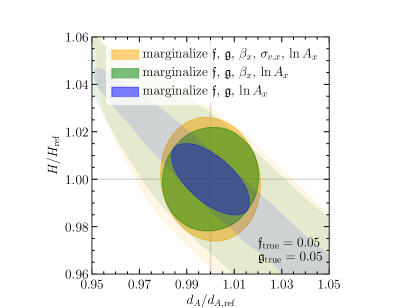
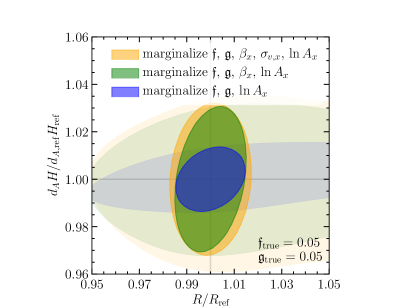
Figure 14: Results from the joint-analysis method: Left: $1\sigma$ ($68\text{\,}\mathrm{\char 37\relax}$ C.L.) uncertainties on $d_{A}$ and $H$ at the LAE redshift when $\mathfrak{f}_{\mathrm{true}}=\mathfrak{g}_{\mathrm{true}}=$5\text{\,}\mathrm{\char 37\relax}$$. The strongly shaded ellipses correspond to Case C where the shape of the LAE power spectrum is known and we fit for the 1D OIIE power spectrum. The lightly shaded ellipses are the constraints for Case D when fitting both the 1D LAE and 1D OIIE power spectra. The color coding indicates which parameters are marginalized over, as described in the legend. Right: Projected constraints for the same cases as the left panel, but for $R=(d_{A}^{2}/H)^{1/3}$ and $AP=d_{A}H$.

Now we examine the case when we relax the assumption that the 1D LAE power spectrum shape is known. Without the shape information, we cannot measure $R=(d_{A}^{2}/H)^{1/3}$. However, the Alcock-Paczynski test still allows measurement of the parameter $AP=d_{A}H$ from the anisotropy of the redshift-space power spectrum. Here, in order to highlight this point, we exclude the shape information altogether, including the BAO that must enhance the constraint on $R$.

We model the LAE power spectrum similarly to the way we modeled the OIIE power spectrum: $P_{L}(k)$ will be a $3^{\text{rd}}$-order spline with knots linearly spaced for $k<$0.04\text{\,}\mathrm{\text{$h$}}\text{\,}{\mathrm{Mpc}}^{-1}$$ and logarithmically spaced for $$0.04\text{\,}\mathrm{\text{$h$}}\text{\,}{\mathrm{Mpc}}^{-1}$<k<$0.4\text{\,}\mathrm{\text{$h$}}\text{\,}{\mathrm{Mpc}}^{-1}$$. This approach is adopted to ensure that all major features of the power spectrum can be represented by the fit. Without a dedicated search for the BAO (Koehler et al., 2007; Shoji et al., 2009), however, we cannot measure $R$.

The left hand side of Fig. 14 shows the projected constraints on $d_{A}$ and $H$ when $\mathfrak{f}=\mathfrak{g}=5\%$, after marginalizing over the interloper fraction and the amplitude (Case C, strongly shaded blue) or the full 1D power spectrum (Case D, lightly shaded blue). For the green and orange ellipses we additionally marginalize over the RSD and FoG parameters, respectively. The figure reveals the degeneracy between $d_{A}$ and $H$ along the direction of constant $AP=d_{A}H$, as shown in the right panel in Fig. 14. When the shape of the LAE power spectrum is completely unknown, HETDEX can still measure $d_{A}H$ to about $3\text{\,}\mathrm{\char 37\relax}$ accuracy.

4.7 Effect of higher-order RSD

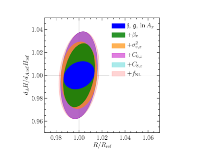
Figure 15: Results from the joint-analysis method, Case B: $1\sigma$ (68% C.L.) uncertainty ranges on $R$ and $d_{A}H$, successively marginalizing over more parameters as indicated in the legend. Whenever a parameter has an $x$ suffix, it means that we marginalize over both the parameter for LAEs and for OIIEs.

We have used Eq. (24) for modeling the redshift-space distortions, including the linear theory prediction (Kaiser effect) and the Finger-of-God suppression. In this section, we study the effect from the non-linear contribution of redshift space distortion. To fully account for the nonlinear distortion in a consistent manner, we need to include the full perturbation theory expression in, for example, Desjacques et al. (2018b). For the purpose of testing the interplay between the interloper fraction and the nonlinear RSD effect on the distance measurement ($R$ and $d_{A}H$), however, we develop an ansatz motivated by the full expression. Specifically, we add parameters $C_{6}^{L}$, $C_{6}^{O}$ and $C_{8}^{L}$, $C_{8}^{O}$ to account for the higher-order angular dependence, replacing Eq. (24) by

$$P_{x}(k_{\perp},k_{\parallel}) =A_{x}^{2}\,A_{\mathrm{RSD}}(k,\mu)\,A_{\mathrm{FoG}}(k,\mu)\,P_{x}^{\text{lin}}(k)\,,$$ (45)

where

$$P_{x}^{\mathrm{lin}}(k) =b_{x}^{2}\,D^{2}(z_{x})\,P_{m}^{\mathrm{lin}}(k)$$ (46)

$$A_{\mathrm{RSD}}(k,\mu) =\big{[}1+2\beta_{x}\mu^{2}+\beta_{x}^{2}\mu^{4}$$

$$\quad+C_{6}^{x}b_{x}^{-2}\sigma_{v,x}^{2}k^{2}\mu^{6}+C_{8}^{x}b_{x}^{-2}\sigma_{v,x}^{2}k^{2}\mu^{8}\big{]}$$ (47)

$$A_{\mathrm{FoG}} =\left(1+f^{2}k^{2}\mu^{2}\sigma_{v,x}^{2}\right)^{-1}\,.$$ (48)

This parametrization naturally reduces to the linear Kaiser formula Eq. (24) in the large-scale limit $k\to 0$. We study the projected constraints with fiducial values of $C_{6}=C_{8}=0$ (under the null hypothesis); increasing them to $C_{6}=C_{8}=1$ does not change the result significantly.

Fig. 15 presents the projected constraints on $R$ and $d_{A}H$ as we marginalize over successively more parameters, assuming that the shape of both LAE and OIIE power spectra are known. Including the nonlinear redshift-space distortion does not affect the projected constraint on the $R$ parameter which controls the isotropic shift of the wavenumbers because the features in the monopole galaxy power spectrum such as the BAO provide information orthogonal to the anisotropies. Conversely, the Alcock-Paczynski test is weakened by the marginalization over $C_{6}$. When marginalizing over the $C_{8}$ parameter, however, there is no noticeable difference.

4.8 Interloper bias and primordial non-Gaussianity

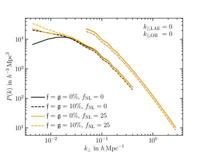
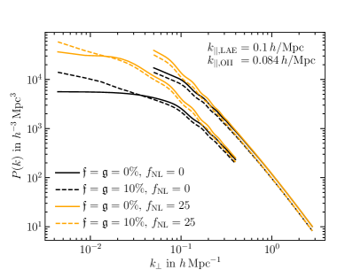
Figure 16: Here we show the power spectrum with and without interlopers and with and without primordial non-Gaussianity (parameterized by $f_{\mathrm{NL}}$) for the HETDEX survey. Top: At $k_{\parallel}=0$ interlopers and $f_{\mathrm{NL}}$ change the power spectrum in similar ways. Bottom: At $k_{\parallel}\neq 0$, the non-Gaussianity introduces a $k$-dependence different from interlopers.

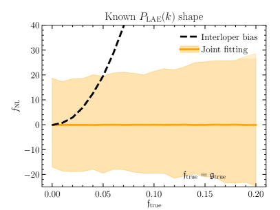
Figure 17: The dashed black line indicates the interloper bias in $f_{\mathrm{NL}}$ when interlopers are ignored, while the orange line is the result of our joint fitting method. In both cases, the fiducial $f_{\mathrm{NL}}=0$. The shaded area represents the $1\sigma$ ($68\text{\,}\mathrm{\char 37\relax}$ C.L.) range calculated from the MCMC chain using the galaxy power spectrum. We use our Case C calculation (Sec. 4.5), marginalizing over the interloper fractions ($\mathfrak{f}$ and $\mathfrak{g}$), angular diameter distance ($d_{A}$), Hubble expansion rate ($H$), amplitude of LAE power spectrum ($\ln A_{L}$), 1D OIIE power spectrum, and RSD and FoG parameters.

Inspection of the interloper effect on the monopole and quadrupole power spectra in Fig. 4 suggests that at large scales the lower redshift interlopers generically add significant power to the power spectrum of the main higher-redshift sample. This behavior arises because the small-scale interloper power spectrum is boosted and added to the main sample power spectrum. Also, the scale-dependent addition to the power spectrum on large scales is the characteristic feature of the scale-dependent bias from primordial non-Gaussianities (Dalal et al., 2008; Desjacques et al., 2018a). In this section, we study the effect of interlopers on measuring the primordial non-Gaussianity parameter $f_{\mathrm{NL}}$ of local type (Salopek & Bond, 1990; Komatsu & Spergel, 2001).

The scale-dependent bias generated from local-type primordial non-Gaussianity adds to the linear bias $b_{x}$ ($x=L$ and $x=O$ for, respectively, LAEs and OIIEs) as

$$\Delta b_{x}(k)=f_{\mathrm{NL}}\,2\,\delta_{c}\,(b_{x}-1)\,\frac{3\Omega_{m}H_{0}^{2}}{2k^{2}T(k)D_{\rm md}(z)}\,,$$ (49)

where $f_{\mathrm{NL}}$ is the nonlinearity parameter, $\delta_{c}=1.686$ is the critical density contrast in the spherical collapse model, $\Omega_{m}$ is the present-day matter density parameter, $H_{0}$ is the Hubble constant, $T(k)$ is the transfer function, and $D_{\rm md}(z)$ is the linear growth function normalized to the scale factor $a$ during the matter-dominated epoch.

As is clear in Eq. (49), for a positive nonlinearity parameter $f_{\mathrm{NL}}$, the scale-dependent bias increases the power at large scales; this behavior is similar to the effect of interlopers. Fig. 16 demonstrates this point by comparing the LAE power spectrum without interlopers (solid lines) and with $10\text{\,}\mathrm{\char 37\relax}$ interlopers (dashed lines). The black lines are for $f_{\mathrm{NL}}=0$ while the orange lines are for $f_{\mathrm{NL}}=25$. The top and bottom panels differ in the value of $k_{\parallel}$ that is fixed, as indicated in the figure. The top panel of Fig. 16 reveals that interlopers have a similar effect as a positive $f_{\mathrm{NL}}$. The bottom panel of Fig. 16, however, shows that the scale-dependence from non-Gaussianities are distinct from the scale-dependence from interlopers for different $k_{\parallel}$, i.e., the scale-dependence of the interloper contamination has a distinctive angular dependence from the isotropic scale-dependence of the local primordial non-Gaussianity.

We first test the effect of primordial non-Gaussianities on the distance measurement in Fig. 15. The projected uncertainties on $R$ and $d_{A}H$, after marginalizing over the nonlinearity parameter $f_{\mathrm{NL}}$, slightly increase along the $R$ direction.

The fact that the interloper effect and primordial non-Gaussianity produce similar scale-dependencies in the galaxy power spectrum causes larger interloper bias. Fig. 17 shows the interloper bias in $f_{\mathrm{NL}}$ when ignoring the interlopers (dashed black line) and compares it with the result from the joint fitting method (solid orange). Thus, non-Gaussianity can be distinguished from interlopers, and, once again, Fig. 17 clearly demonstrates that the joint fitting method removes the interloper bias.

5 Statistical analysis for WFIRST

Figure 18: A schematic indicating how we divide the H$\alpha$ and [O III] samples to avoid overlap in our joint fitting method applied to the WFIRST mission. We split the spectrum into three wavelength ranges A ($1.35\,{\rm\mu m}<\lambda_{\mathrm{obs}}<1.44\,{\rm\mu m}$), B ($1.44\,{\rm\mu m}<\lambda_{\mathrm{obs}}<1.77\,{\rm\mu m}$), and C ($1.77\,{\rm\mu m}<\lambda_{\mathrm{obs}}<1.89\,{\rm\mu m}$), corresponding to the redshift ranges for H$\alpha$ and [O III] as shown in the figure. In region A, an [O III] line is identified by the simultaneous presence of H$\alpha$ in the spectrum. Thus, in region A the absence of a second line identifies H$\alpha$. Similarly, in region C we either expect to see both lines, or else it must be [O III]. In region B only one of the two lines is present at a time, and thus we expect misidentification to be a potential problem where our method fitting for $\mathfrak{f}$ and $\mathfrak{g}$ may be needed.

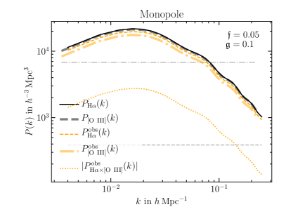
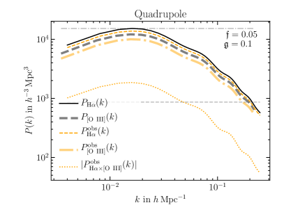
Figure 19: Monopole (left) and quadrupole (right) for the WFIRST galaxy samples. The black solid line represents the H$\alpha$ power spectrum; the thick grey dashed shows the [O III] power spectrum without interlopers. The thin orange dashed line indicates the H$\alpha$ samples with $\mathfrak{f}=0.05$ interlopers, while the thick orange dash-dotted line shows [O III] with $\mathfrak{g}=0.1$ interlopers. The horizontal grey dashed line shows the shot noise for the H$\alpha$ sample, the dashed-dotted line is the same for the [O III] sample. The orange dotted line is the cross-correlation in the presence of interlopers. In all cases the main effect from interlopers is to reduce the power by a constant factor.

In this section, we apply the joint fitting method to the planned High Latitude Spectroscopic Survey of NASA’s Wide-Field Infrared Survey Telescope (WFIRST) mission (Spergel et al., 2015). WFIRST is an emission-line galaxy survey using slitless grism spectroscopy in the infrared wavelength range between $1.351.89\text{\,}\mathrm{\SIUnitSymbolMicro m}$ with spectral resolution of $R\equiv\lambda/\Delta\lambda\simeq$620870$$. The total sky area coverage of the survey is $2200\text{\,}\mathrm{d}\mathrm{e}\mathrm{g}\mathrm{{}^{2}}$ ($f_{\rm sky}\simeq 0.05$) for which we can safely apply the Fourier-based analysis method in the previous section.

Focusing on the two largest emission line samples, we consider the main galaxy sample of H$\alpha$ ($\lambda$6563Å) emitters (HAEs) contaminated by [O III] ($\lambda$5007Å) emitters (OIIIEs). With the wavelength coverage of the survey, the observed HAEs will be in the redshift range $1.05<z<1.88$, and the observed OIIIEs will be at $1.70<z<2.77$.

We assume that the line intensities for both H$\alpha$ and [O III] are strong for all emission-line galaxies at the redshift range of WFIRST. This is motivated by Bowman et al. (2018). Using the 3D-HST grism data (Brammer et al., 2012; Skelton et al., 2014; Momcheva et al., 2016), they find that both lines are strong at $z\sim 2$. However, in the local universe, [O III] is often weak. Thus, our assumption may turn out to be an optimistic one. A proper solution would take into account the sample of [O II] emitters and other lines that may be present in the spectrum. We leave this to a future investigation.

The assumption of both lines being strong implies two important points for the line identification. First, in the overlapping redshift range $1.7<z<1.88$, both H$\alpha$ and [O III] lines will be observed and the HAE sample coincides with the OIIIE sample; the presence of a second line unambiguously identifies the sample. Second, for the lower redshift ($1.05<z<1.20$) HAEs, the interpretation is unambiguous; if we identified the line as [O III], the corresponding H$\alpha$ must be detected as well. Similarly, the line identification for the higher redshift ($2.54<z<2.77$) OIIIEs is also unambiguous.

The relation between the H$\alpha$ and [O III] redshift bins is illustrated in Fig. 18, where we identify three regions in the spectrum; for the main HAE sample: $1.05<z<1.2$, $1.2<z<1.7$, and $1.7<z<1.88$; for the interloper OIIIE sample: $1.7<z<1.88$, $1.88<z<2.54$ and $2.54<z<2.77$. For both cases, we assume no interloper for the first and the third bins. For the middle bins ($1.2<z<1.7$ for HAEs and $1.88<z<2.54$ for OIIIEs) we apply our method of measuring the interloper fractions $\mathfrak{f}$ (OIIIEs contaminating HAEs) and $\mathfrak{g}$ (HAEs contaminating OIIIEs) from the cross-correlation. The HAEs and OIIIEs coincide in the overlapping region ($1.7<z<1.88$) that we analyze only once.

For the Fourier analysis, we use the central redshifts of each of the bins to calculate the geometrical quantities. For HAEs, the survey volume for each bin is $V_{\text{survey}}^{\text{lo}}=$0.92\text{\,}{\mathrm{\text{$h$}}}^{-3}\text{\,}{\mathrm{Gpc}}^{3}$$ (for the low-$z$ bin), $V_{\text{survey}}^{\text{mid}}=$3.87\text{\,}{\mathrm{\text{$h$}}}^{-3}\text{\,}{\mathrm{Gpc}}^{3}$$ (for the middle-$z$ bin), and $V_{\text{survey}}^{\text{hi}}=$1.53\text{\,}{\mathrm{\text{$h$}}}^{-3}\text{\,}{\mathrm{Gpc}}^{3}$$ (for the high-$z$ bin). For OIIIEs, they are $V_{\text{survey}}^{\text{OIIIE,lo}}=$1.67\text{\,}{\mathrm{\text{$h$}}}^{-3}\text{\,}{\mathrm{Gpc}}^{3}$$, $V_{\text{survey}}^{\text{OIIIE,mid}}=$5.77\text{\,}{\mathrm{\text{$h$}}}^{-3}\text{\,}{\mathrm{Gpc}}^{3}$$, and $V_{\text{survey}}^{\text{OIIIE,hi}}=$2.09\text{\,}{\mathrm{\text{$h$}}}^{-3}\text{\,}{\mathrm{Gpc}}^{3}$$. For the number of samples, we use 16.4 million HAEs and 1.4 million OIIIEs and adopt the linear galaxy bias of $b_{\mathrm{HAE}}=1.5$ and $b_{\mathrm{OIII}}=2$ (Spergel et al., 2015). We spread the galaxies uniformly over the survey volume to calculate the number densities for HAEs and OIIIEs. Just like for HETDEX, we project the OIIIEs onto the HAE redshift for the Fourier analysis. The scaling factors in our reference cosmology are $\alpha=0.78$, $\beta=1.10$. We use all Fourier modes below the maximum wavenumber $k_{\perp,\mathrm{max}}=k_{\parallel,\mathrm{max}}=$0.25\text{\,}\mathrm{\text{$h$}}\text{\,}{\mathrm{Mpc}}^{-1}$$ at the HAE redshift. Because the HAEs and OIIIEs are at high redshifts, we assume that both HAE and OIIIE galaxy power spectra are well modeled by a theoretical template. This assumption corresponds to the Case B of Sec. 4.4. As for the baseline model, we use the expression in Eq. (24).

Finally, after the analysis for each bin, we combine the result by adding the Fisher information matrices. The combined center redshifts are $z_{\mathrm{HAE}}=1.47$ and $z_{\rm OIIIE}=2.32$. We count the galaxies in the overlapping range ($1.70<z<1.88$) as a part of the main HAE sample. For our baseline analysis, we marginalize over the amplitudes of the HAE and OIIIE power spectra, the angular diameter distances and the Hubble expansion rates at $z_{\mathrm{HAE}}$ and $z_{\mathrm{OIII}}$, the RSD parameters ($\beta_{x}$), and the FoG velocity dispersions ($\sigma_{v,x}^{2}$).

5.1 Power spectra

The monopole and quadrupole of the observed galaxy power spectra along with the contribution from contaminants (for $\mathfrak{f}=0.05$ and $\mathfrak{g}=0.1$) are presented in Fig. 19. The interloper contribution is quite different from the case for HETDEX (shown in Fig. 4) because the WFIRST HAEs (the main sample) and OIIIEs (the interlopers) are at similar redshifts, which makes the projection parameters $\alpha\sim 0.78$ and $\beta\sim 1.1$ close to unity.

The main effect is, therefore, to suppress the observed power spectra of HAEs and OIIIEs by the factors of $(1-\mathfrak{f})^{2}$ and $(1-\mathfrak{g})^{2}$ [see Eq. (18) and Eq. (20), and replace LAE with HAE and OII with OIII]. Since the contributions from the contaminants are suppressed by the square of the contamination fraction and the volume factor $\alpha^{2}\beta=0.67$ is of order unity, the observed power spectra are mainly affected by a change in their amplitude. The products of the linear galaxy bias and growth factor for the HAE and OIIIE samples are quite similar, so their uncontaminated monopole power spectra lie nearly on top of each other.

Because the contamination effect is quite minor in the auto-power spectra of HAEs and OIIIEs, we expect that the cross-power spectrum is the main driver for the measurement of the contamination fractions $\mathfrak{f}$ and $\mathfrak{g}$ (see Fig. 21 below).

5.2 Interloper bias

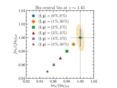
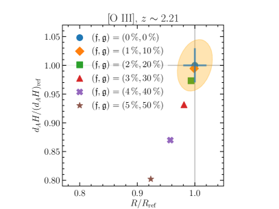
Figure 20: Top: When the presence of interlopers is ignored, the measurements of $f\sigma_{8}$ and $b\sigma_{8}$ will be biased. This is primarily due to the reduction in power from the factor $(1-\mathfrak{f})^{2}$ in Eq. (18), as applied to WFIRST. To show that the interloper bias does not depend on the fraction $\mathfrak{g}$, we set $\mathfrak{g}=$50\text{\,}\mathrm{\char 37\relax}$$ for the $\mathfrak{f}=$1\text{\,}\mathrm{\char 37\relax}$,$5\text{\,}\mathrm{\char 37\relax}$$ cases. Bottom: Although there is no interloper bias for the HAE distance measurements, the distances $d_{A}H$ and $R$ measured from the OIIIEs (at $z\sim 2.21$) will be biased without a proper account of the HAE interloper effect.

We estimate the systematic changes in the maximum-likelihood value of cosmological parameters $p_{i}$ due to the interloper contamination by using

$$\Delta p_{i} =\bar{F}^{-1}_{ij}\sum_{\bm{k}}\frac{N_{\bm{k}}}{2}\,\frac{P_{,j}({\bm{k}};\bar{p}_{i})}{P({\bm{k}};\bar{p}_{i})}\,\frac{\Delta\hat{P}({\bm{k}})}{P({\bm{k}};\bar{p}_{i})}\,,$$ (50)

where $\bar{F}_{ij}$ is the Fisher information matrix, and $\Delta\hat{P}({\bm{k}})$ is the change in the power spectrum due to interlopers. We give the derivation of Eq. (50) in App. D.

Let us first consider the interloper bias for the main HAE sample. From Eq. (18) this is

$$\Delta\hat{P}_{\rm HAE}({\bm{k}}) =-\mathfrak{f}\,(2-\mathfrak{f})P_{\mathrm{HAE}}({\bm{k}})+\mathfrak{f}^{2}P_{\mathrm{OIII}}^{\mathrm{proj}}({\bm{k}})\,.$$ (51)

Since the OIIIE power spectrum gets projected into a smaller volume ($\alpha^{2}\beta\sim 0.67$) and the interloper fraction $\mathfrak{f}$ is smaller than $\mathfrak{f}_{\rm lim}=\bar{N}_{\mathrm{OIII}}/(\bar{N}_{\mathrm{HAE}}+\bar{N}_{\mathrm{OIII}})=0.079$ (see App. A), the second term in Eq. (51) must be negligible compared to the first term. The main interloper effect on the HAE power spectrum, therefore, is to change the observed amplitude. We have also indicated this effect in Fig. 19.

Because the interloper contamination does not distort the shape of the power spectrum, we forecast that there will be no significant interloper bias for the measurement of the angular diameter distance and the Hubble expansion rate at the HAE redshift.

On the other hand, both $f\sigma_{8}$ and $b\sigma_{8}$ (two direct observables from the dynamical measurement of redshift-space distortion) would be systematically biased if the presence of interlopers is ignored. We show this in the top panel of Fig. 20 for five different values for the interloper fractions. This figure is similar to Fig. (4) in Pullen et al. (2016), but for the direct observables from the two-dimensional galaxy power spectrum. From the Figure it is apparent that the interloper bias in the $b\sigma_{8}$-$f\sigma_{8}$ plane is quite strongly correlated, and the correlation is due to the bias in the amplitude of the observed galaxy power spectrum.

For the OIIIE samples, the story is quite different. Because the contamination fraction can be as high as $g_{\rm lim}=\bar{N}_{\mathrm{HAE}}/(\bar{N}_{\mathrm{HAE}}+\bar{N}_{\mathrm{OIII}})=0.92$, a small leakage of HAEs into the OIIIE sample can generate significant interloper bias for the distance measurement. We show this in the bottom panel of Fig. 20. Here, we fix the ratio $\mathfrak{f}/\mathfrak{g}=0.1$ to reflect the sample size ratio between HAEs and OIIIEs.

5.3 Joint fitting

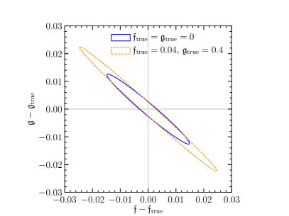
Figure 21: The result of the joint-analysis method: $1\sigma$ (68% C.L.) constraints for WFIRST on the interloper fractions $\mathfrak{f}$ and $\mathfrak{g}$ for $\mathfrak{f}_{\mathrm{true}}=\mathfrak{g}_{\mathrm{true}}=0$ (solid blue ellipse) and $(\mathfrak{f}_{\mathrm{true}},\mathfrak{g}_{\mathrm{true}})=($4\text{\,}\mathrm{\char 37\relax}$,\,$40\text{\,}\mathrm{\char 37\relax}$)$ (dashed orange ellipse). We assume Case B.

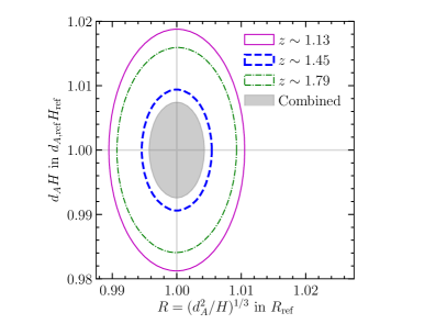
Figure 22: Results from the joint-analysis method: projected $1\sigma$ (68% C.L.) range for $R$ and $d_{A}H$ for WFIRST, assuming Case B. The solid magenta ellipse shows the confidence interval from the lowest redshift bin assuming no misidentification, the thick dashed blue ellipse from the center redshift bin marginalizing over interloper fractions, and the dash-dotted green ellipse shows the confidence interval from the highest redshift bin again assuming no misidentification. The grey shaded ellipse shows the combined constraint from all three bins. Here, $\mathfrak{f}_{\mathrm{true}}=\mathfrak{g}_{\mathrm{true}}=0$.

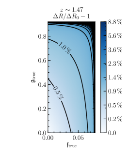
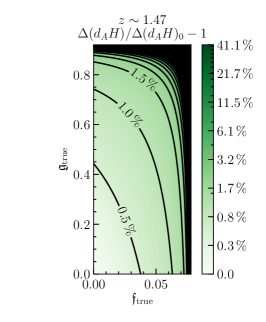
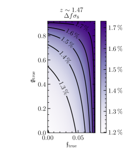
Figure 23: Left: Results from the joint-analysis method: the forecast for the relative change in the $1\sigma$ (68% C.L.) uncertainty on $R$ at the H$\alpha$ redshift as a function of the true $\mathfrak{f}$ and $\mathfrak{g}$ for WFIRST. Since the expected ratio of HAEs to OIIIEs is $\sim 12$, the limiting interloper fractions are $\mathfrak{f}_{\mathrm{lim}}=0.079$ and $\mathfrak{g}_{\mathrm{lim}}=0.92$. Note that for easier display the abscissa is on a larger scale than the ordinate. We forecast the best constraint to be $\Delta R_{0}=0.28\%$ at $\mathfrak{f}=\mathfrak{g}=0$. The forecast measurement uncertainty $\Delta R$ changes by less than a percent over most of the plot. Center: Similar to the left plot, but for the change in the uncertainty on the $AP$ parameter $d_{A}H$, starting with $\Delta(d_{A}H)_{0}=$0.49\text{\,}\mathrm{\char 37\relax}$$. Right: Here we show the expected constraints on $f\sigma_{8}$, the best constraints being $\Delta(f\sigma_{8})_{0}=$1.2\text{\,}\mathrm{\char 37\relax}$$ at $\mathfrak{f}=\mathfrak{g}=0$. In alls plots we assume Case B.

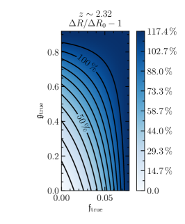
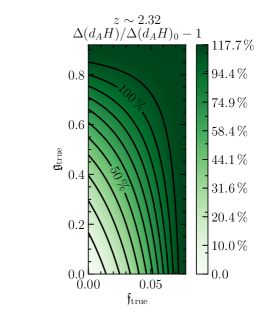
Figure 24: Similar to Fig. 23 here we show our forecast for the relative change in the uncertainty on $R$ (left) and $dA_{H}$ (center) as a function of the true $\mathfrak{f}$ and $\mathfrak{g}$ for WFIRST, and the uncertainty on $f\sigma_{8}$ (right) at the redshift of the [O III] emitters. We forecast the best constraint to be $\Delta R_{0}=0.89\%$ at $\mathfrak{f}=\mathfrak{g}=0$, $\Delta(d_{A}H)_{0}=$1.8\text{\,}\mathrm{\char 37\relax}$$, and $\Delta(f\sigma_{8})_{0}=$3.82\text{\,}\mathrm{\char 37\relax}$$. In alls plots we assume Case B.

Figure 25: Results from the joint-analysis method: $1\sigma$ (68% C.L.) range on $f_{\mathrm{NL}}$ as a function of interloper fractions ($\mathfrak{f}_{\mathrm{true}}$, $\mathfrak{g}_{\mathrm{true}}$). To constrain $f_{\mathrm{NL}}$ we only consider the galaxy power spectrum, combining five bins: the three H$\alpha$ bins, and the upper two [O III] bins. We assume Case B.

In this section, we apply the joint analysis technique to WFIRST. That is, we use all three power spectra (HAE power spectrum, OIIIE power spectrum and HAE-OIIIE cross power spectrum) as observables to estimate the cosmological parameters, and show that the parameters estimated from the joint analysis are unbiased.

First, Fig. 21 shows the projected constraints for the interloper fractions $\mathfrak{f}$ and $\mathfrak{g}$ for two sets of interloper fractions. Compared to HETDEX (Fig. 9), the measurement uncertainty on the interloper fractions $\mathfrak{f}$ and $\mathfrak{g}$ is larger and they are more highly correlated. This is explained by the fact that the two samples are closer in redshift, and so the two power spectra have less distinct signals in the cross-correlation. This plot shows that we can measure a percent level interloper fraction from the cross power spectrum of WFIRST .

With our joint-analysis method the interloper bias on $f\sigma_{8}$ and the distance measures shown in Fig. 20 is removed. For the H$\alpha$ sample we forecast $\sim 1.5\text{\,}\mathrm{\char 37\relax}2\text{\,}\mathrm{\char 37\relax}$ constraints, and for the [O III] sample $\sim 4.5\text{\,}\mathrm{\char 37\relax}7\text{\,}\mathrm{\char 37\relax}$ for interloper fraction $\mathfrak{g}_{\mathrm{true}}\lesssim$30\text{\,}\mathrm{\char 37\relax}$$, and higher for larger interloper fractions.

In Fig. 22 we show the projected constraints on $R$ and $d_{A}H$ for all three bins when the true interloper fractions vanish. The bins are labeled in the legend by their central redshifts. We marginalize over the amplitude, RSD, and FoG parameters for all three bins. For the central bin we additionally marginalize over $\mathfrak{f}$, $\mathfrak{g}$, and the amplitude, RSD, and FoG parameter of the corresponding OIIIE sample. The constraints largely reflect the size of the survey volume. The weakest constraints come from the bin with the smallest volume, the most tight constraints from the bin with the largest volume. The grey shaded ellipse shows the constraints combining all three bins assuming they are statistically independent. Combined, we get $\sim 0.28\text{\,}\mathrm{\char 37\relax}$ uncertainty on $R$. This is more optimistic than Spergel et al. (2015) since we model the full shape of the power spectrum, including the broadband shape.

On the left of Fig. 23 we show how the projected uncertainty on $R$ measured from the HAE sample relative to the best case (without contamination, at $\mathfrak{f}=\mathfrak{g}=0$) changes as a function of the contamination fractions $\mathfrak{f}$ and $\mathfrak{g}$. Since the fiducial ratio of OIIIEs to HAEs is $\sim 12$, the limiting interloper fractions are $(\mathfrak{f}_{\mathrm{lim}},\mathfrak{g}_{\mathrm{lim}})=(0.079,0.92)$. Note that to better show the lower allowed region, the abscissa has been stretched compared to the ordinate. We neglect the upper allowed region that corresponds to catastrophic misidentification. At $(\mathfrak{f}_{\mathrm{true}},\mathfrak{g}_{\mathrm{true}})=(0,0)$ the constraint is $\Delta R_{0}=$0.28\text{\,}\mathrm{\char 37\relax}$$. The constraint changes by less than $1\text{\,}\mathrm{\char 37\relax}$ for most of the lower allowed region before increasing rapidly near the limiting fractions. Similarly, the center panel of Fig. 23 shows the change in the projected uncertainties for the $AP$ parameter $d_{A}H$ as a function of $\mathfrak{f}$ and $\mathfrak{g}$. Here, the best constraint is $\Delta(d_{A}H)_{0}=$0.49\text{\,}\mathrm{\char 37\relax}$$. The right panel of Fig. 23 shows the uncertainty on $f\sigma_{8}$ for the HAE sample. The best constraint we get with marginalization over the interloper fractions is $\sim 1.2\text{\,}\mathrm{\char 37\relax}$.

Fig. 24 shows the same combining the upper two [O III] bins. Note that we do not include the lowest [O III] bin, as we assume that the OIIIEs of the lowest redshift bin are already included with the HAEs in their highest redshift bin. On the left of the figure, we show the change of the uncertainty relative to the best case $\Delta R_{0}=$0.89\text{\,}\mathrm{\char 37\relax}$$, in the center, the change relative to $\Delta(d_{A}H)_{0}=$1.8\text{\,}\mathrm{\char 37\relax}$$, and on the right the uncertainty on $f\sigma_{8}$, which we forecast to be $\Delta f\sigma_{8}\sim$3.8\text{\,}\mathrm{\char 37\relax}$$ in the ideal case.

Finally, in Fig. 25 we show forecasts for the non-Gaussianity parameter $f_{\mathrm{NL}}$. We only consider the constraint from the galaxy power spectrum, combining the information from both HAEs and OIIIEs. From the galaxy power spectrum alone, we forecast $\Delta f_{\mathrm{NL}}\sim$1216$$ for WFIRST after marginalizing over all nuisance parameters, with a best-case $\Delta f_{\mathrm{NL}}=11.7$ at zero interloper fractions.

6 Conclusion

In this paper, we study the effects of interlopers in the cosmological analysis based on the power spectrum measured from emission-line galaxy surveys. In particular, the paper focuses on the two relatively narrow field surveys HETDEX and WFIRST.

For HETDEX, we define the interloper fraction $\mathfrak{f}$ of the Lyman-$\alpha$ emitter (LAE) sample and the interloper fraction $\mathfrak{g}$ of the [O II] emitter (OIIE) sample in Eqs. (4)–(5). For WFIRST, we define $\mathfrak{f}$ to be the interloper fraction in the H$\alpha$ sample, and $\mathfrak{g}$ the interloper fraction in the [O III] sample. We then derive the effect of interlopers on the power spectrum in Eq. (18), Eq. (20), and Eq. (22). The change in the power spectrum is given in terms of two geometrical factors defined in Eq. (7): the direction perpendicular to the line-of-sight gets scaled by the factor $\alpha$, while the direction parallel scales by the factor $\beta$. For the two surveys that we study, $\alpha\neq\beta$, and thus the projection introduces anisotropies in the two-dimensional galaxy power spectrum, in addition to redshift-space distortions. The volume factor $\alpha^{2}\beta$ also multiplies the contamination contribution from the interloper power spectrum. In App. B, we also provide the rigorous derivation of the shot noise under the assumption that the galaxies are a Poisson sample of the underlying continuous galaxy density field, and the interloper fraction plays the role of the probability of having contamination.

We then investigate the joint-analysis method including auto-power spectra of both samples as well as the cross-power spectrum as observables. We show that the joint analysis yields robust measurements of the interloper fractions and it removes the interloper bias, a systematic shift of the best-fitting cosmological parameters when ignoring the interlopers. Although measuring and marginalizing the interloper fractions increases the measurement uncertainties in cosmological parameters, it does not bias their maximum likelihood values. We explicitly show this for the geometrical parameters (angular diameter distance and Hubble expansion parameter) as well as the dynamical parameters (linear growth rate and $\sigma_{8}$), higher-order RSD parameters (Sec. 4.7), and non-Gaussianity (Sec. 4.8).

For the joint-analysis, we investigate several models for the power spectra of the main survey galaxies and the interlopers. We consider four cases:

Case A

This case makes minimal assumptions, only assuming that the true cross-correlation vanishes, see Sec. 4.3.

Case B

This case makes maximal assumptions, assuming that the redshift-space distortions and the shapes of the 1D isotropic power spectra are well-modeled by theory, see Sec. 4.4.

Case C

Similar to Case B, but we only asssume to be able to model the isotropic auto-correlation power spectrum of the higher-redshift sample, see Sec. 4.5.

Case D

Here we assume we can model only the redshift-space distortions of the two samples, see Sec. 4.6.

By doing a Fisher analysis, we show that the constraints on the interloper fractions $\mathfrak{f}$ and $\mathfrak{g}$ are essentially the same for the two extreme cases A and B (see Fig. 9), confirming that the information comes primarily from the cross-correlation.

Naturally, there is a large continuum of intermediate cases, and it needs to be assessed on a survey-by-survey basis which one to use. For HETDEX, while the main LAE samples probe the quasi-linear scales at high redshift, the interlopers are at low redshift and probe scales deep into the nonlinear regime. Thus, we assume Case C as the baseline, where we marginalize over the 1D OIIE power spectrum. For WFIRST, we take Case B as the baseline, because both the main sample and interloper sample probe the quasi-linear scales at high redshifts.

This paper shows that the better the line classification, the tighter we can constrain the cosmological parameters. For the astrophysical methods of line classification, our joint-analysis method provides an estimate of the total contamination fractions. The usual approach to compliment the emission line surveys is to have follow-up imaging data in the same survey footprint. For HETDEX, Leung et al. (2017) developed a Bayesian framework taking into account the equivalent width distribution of LAEs and OIIEs, and searching for other lines that may be present in the spectrum. For WFIRST, Pullen et al. (2016) investigated the use of sensitive photometric data. All of these methods work for the classification of individual emission-line galaxies. The estimated interloper fractions from the joint analysis then provide a global figure of merit, based on which we can modify the line identification criteria to reach smaller interloper fractions. The interplay between the two methods will provide a way to optimize the analysis pipeline for the emission-line galaxy surveys.

Although we have not investigated further, one can also incorporate cross-correlations with external datasets. For example, for HETDEX, low-redshift galaxy samples from SDSS (Eisenstein et al., 2011) that correlate with the OIIE sample should provide an extra constraint on the contamination fraction $\mathfrak{g}$ when cross-correlating the low-redshift galaxies with the high-redshift LAEs.

Although we have not investigated further, one can also incorporate cross-correlations with external datasets. For example, for HETDEX, low-redshift galaxy samples from SDSS (Eisenstein et al. 2011), or radio catalogs from LOFAR (Shimwell et al., 2019), or APERTIF (Adams et al., 2018) that correlate with the OIIE sample should provide an extra constraint on the contamination fraction g when cross-correlating the low-redshift galaxies with the high-redshift LAEs.

The results of this paper required two key simplifying assumptions: a flat-sky approximation and no redshift evolution in the interloper fractions, the galaxy bias, or the linear growth rate. To address these caveats in the future and to apply the joint-analysis method to wide-angle galaxy surveys including Euclid and SPHEREx, we must extend the method to spherical harmonic space while incorporating astrophysically motivated assumptions about the redshift evolution of key parameters. For example, Leung et al. (2017) predict the interloper fractions, $\mathfrak{f}$ and $\mathfrak{g}$, as a function of redshift for the LAEs and OIIEs, which could be incorporated in the future.

Appendix A Transformation between misidentification and interloper fractions

Figure 26: Transformation from $(x_{\mathrm{LAE}}^{\mathrm{true}},x_{\mathrm{OII}}^{\mathrm{true}})$ to $(\mathfrak{f}_{\mathrm{true}},\mathfrak{g}_{\mathrm{true}})$ for fixed $r_{\mathrm{true}}=N_{\mathrm{OII}}^{\mathrm{true}}/N_{\mathrm{LAE}}^{\mathrm{true}}$. On the left we show the $x_{\mathrm{LAE}}x_{\mathrm{OII}}$-space, on the right the $\mathfrak{f}\mathfrak{g}$-space. Since counts of galaxies must be positive, the greyed-out regions are physically impossible, as explained in App. A. The limiting values $\mathfrak{f}_{\mathrm{lim}}$ and $\mathfrak{g}_{\mathrm{lim}}$ are given in Eqs. (A1)–(A2). When fixing the observed ratio $r_{\mathrm{obs}}$ [Eq. (A5)] instead of $r_{\mathrm{true}}$, then $\mathfrak{f}$ and $\mathfrak{g}$ are unrestricted, and instead $x_{\mathrm{LAE}}$ and $x_{\mathrm{OII}}$ are limited, as elaborated in the text.

In this appendix, we seek a better understanding of the mapping between the misidentification fractions $x_{\mathrm{LAE}}$ and $x_{\mathrm{OII}}$, and the interloper fractions $\mathfrak{f}$ and $\mathfrak{g}$. We introduced $\mathfrak{f}$ and $\mathfrak{g}$ since they are relevant for relating the true and observed power spectra. However, $x_{\mathrm{LAE}}$ and $x_{\mathrm{OII}}$ are a more natural choice for the process of misidentification. We will assume that the misidentification of LAEs as OIIEs is independent from the misidentification of OIIEs as LAEs. That is, we assume that there are two degrees of freedom describing interlopers.

We assume that when performing a forecast for a survey such as HETDEX, the fiducial values for the true numbers of galaxies $N_{\mathrm{LAE}}$ and $N_{\mathrm{OII}}$ are given, e.g., from previously measured luminosity functions (e.g. Ciardullo et al., 2012). This implies that the true interloper fractions $\mathfrak{f}_{\mathrm{true}}$ and $\mathfrak{g}_{\mathrm{true}}$ cannot take on arbitrary values. For example, for HETDEX, we expect there to be about twice as many OIIEs as LAEs. Therefore, the fraction of OIIEs in the LAE sample cannot exceed 2/3 unless some LAEs are misidentified as well. Hence, it is not possible to have more than 2/3 OIIEs in the LAE sample at the same time as an uncontaminated OIIE sample, given the true numbers of galaxies.

To find which interloper fractions are physical, we consider when either the observed LAE number density or the observed OIIE number density vanishes. Then, Eqs. (4)–(5) implies that the limiting cases are on the two lines $\mathfrak{f}_{\mathrm{true}}=\mathfrak{f}_{\mathrm{lim}}$ and $\mathfrak{g}_{\mathrm{true}}=\mathfrak{g}_{\mathrm{lim}}$, where

$$\mathfrak{f}_{\mathrm{lim}} =\frac{N_{\mathrm{OII}}}{N_{\mathrm{LAE}}+N_{\mathrm{OII}}}\,,$$ (A1)

$$\mathfrak{g}_{\mathrm{lim}} =\frac{N_{\mathrm{LAE}}}{N_{\mathrm{LAE}}+N_{\mathrm{OII}}}=1-\mathfrak{f}_{\mathrm{lim}}\,,$$ (A2)

where the numbers are the true numbers of galaxies. The lines $\mathfrak{f}_{\mathrm{true}}=\mathfrak{f}_{\mathrm{lim}}$ and $\mathfrak{g}_{\mathrm{true}}=\mathfrak{g}_{\mathrm{lim}}$ mark boundaries between allowed and disallowed (unphysical) regions for the interloper fractions. By requiring positive number densities, we find that interloper fractions $\mathfrak{f}_{\mathrm{true}}<\mathfrak{f}_{\mathrm{lim}}$ are unphysical unless $\mathfrak{g}_{\mathrm{true}}<\mathfrak{g}_{\mathrm{lim}}$. Similarly, interloper fractions $\mathfrak{f}_{\mathrm{true}}>\mathfrak{f}_{\mathrm{lim}}$ are unphysical unless $\mathfrak{g}_{\mathrm{true}}>\mathfrak{g}_{\mathrm{lim}}$. Thus, we have two allowed regions and two unphysical regions, as shown in the right panel of Fig. 26, where we use $N_{\mathrm{OII}}/N_{\mathrm{LAE}}=2$. Thus, the true interloper fractions must be chosen from the allowed regions $A_{i}$ or $B_{i}$ shown in the figure.

Fixing the ratio of true numbers $N_{\mathrm{OII}}/N_{\mathrm{LAE}}$, we derive the non-linear transformation between interloper fractions and misidentification fractions from Eqs. (2)–(5) to get

$$\mathfrak{f}_{\mathrm{true}} =\left(1+\frac{1-x_{\mathrm{LAE}}^{\mathrm{true}}}{x_{\mathrm{OII}}^{\mathrm{true}}}\,\frac{N_{\mathrm{LAE}}}{N_{\mathrm{OII}}}\right)^{-1}\,,$$ (A3)

$$\mathfrak{g}_{\mathrm{true}} =\left(1+\frac{1-x_{\mathrm{OII}}^{\mathrm{true}}}{x_{\mathrm{LAE}}^{\mathrm{true}}}\,\frac{N_{\mathrm{OII}}}{N_{\mathrm{LAE}}}\right)^{-1}\,.$$ (A4)

To gain a better understanding of the transformation, we show the possible values for $x_{\mathrm{LAE}}^{\mathrm{true}}$ and $x_{\mathrm{OII}}^{\mathrm{true}}$ in the left panel of Fig. 26. The points $(0,0)$ and $(1,1)$ in $x_{\mathrm{LAE}}x_{\mathrm{OII}}$-space become $(0,0)$ and $(1,1)$ in $\mathfrak{f}\mathfrak{g}$-space. The point $(0,1)$ becomes the line $\mathfrak{f}_{\mathrm{true}}=\mathfrak{f}_{\mathrm{lim}}$ (since $\mathfrak{g}$ is undetermined due to the observed number of OIIEs vanishing in this case) and $(1,0)$ becomes $\mathfrak{g}_{\mathrm{true}}=\mathfrak{g}_{\mathrm{lim}}$ (since the observed number of LAEs vanishes). The points on the diagonal $x_{\mathrm{LAE}}^{\mathrm{true}}+x_{\mathrm{OII}}^{\mathrm{true}}=1$ map onto the single point $(\mathfrak{f}_{\mathrm{lim}},\mathfrak{g}_{\mathrm{lim}})$, because the LAE and OIIE samples have the same fraction of LAEs in each, and thus the observed auto power spectra are the same. Furthermore, we have added three more lines: the diagonal $x_{\mathrm{LAE}}^{\mathrm{true}}=x_{\mathrm{OII}}^{\mathrm{true}}$ becomes the curved line in $\mathfrak{f}\mathfrak{g}$-space, and the dashed and dash-dotted lines, which are curved in $x_{\mathrm{LAE}}x_{\mathrm{OII}}$-space, become diagonals of the allowed regions in $\mathfrak{f}\mathfrak{g}$-space. Finally, for clarity, the sub-regions $A_{i}$ and $B_{i}$ have been labeled in the two panels of Fig. 26 correspondingly.

The reason two regions appear in $\mathfrak{f}\mathfrak{g}$-space is due to fixing the true ratio $N_{\mathrm{OII}}/N_{\mathrm{LAE}}$. However, when measuring the interloper fractions $\mathfrak{f}$ and $\mathfrak{g}$, this ratio cannot be assumed to be known. Rather, it must be viewed as a parameter to be determined in the fit. However, the ratio

$$r_{\mathrm{obs}} \equiv\frac{N_{\mathrm{OII}}^{\mathrm{obs}}}{N_{\mathrm{LAE}}^{\mathrm{obs}}}$$ (A5)

will be known, so that the transformation Eqs. (A3)–(A4) now become

$$x_{\mathrm{LAE}} =\left(1+\frac{1-\mathfrak{f}}{\mathfrak{g}}\,r_{\mathrm{obs}}^{-1}\right)^{-1}\,,$$ (A6)

$$x_{\mathrm{OII}} =\left(1+\frac{1-\mathfrak{g}}{\mathfrak{f}}\,r_{\mathrm{obs}}\right)^{-1}\,,$$ (A7)

where now $r_{\mathrm{obs}}$ is fixed instead of $r_{\mathrm{true}}=N_{\mathrm{OII}}/N_{\mathrm{LAE}}$. This transformation has the same form as Eqs. (A3)–(A4), provided that we switch $x_{\mathrm{LAE}}\leftrightarrow\mathfrak{f}$, $x_{\mathrm{OII}}\leftrightarrow\mathfrak{g}$, and $r_{\mathrm{true}}\to r_{\mathrm{obs}}$. Thus, the picture is reversed: when only $r_{\mathrm{obs}}$ is known, the full plane $0\leq\mathfrak{f}\leq 1$ and $0\leq\mathfrak{g}\leq 1$ is allowed. Indeed, since $r_{\mathrm{true}}$ is allowed to vary it is possible to find that the measured values $\mathfrak{f},\mathfrak{g}$ will be within the unphysical regions. Finally, we note that now there are restrictions on the physically-allowed values for $x_{\mathrm{LAE}}$ and $x_{\mathrm{OII}}$ similar to those for $\mathfrak{f}_{\mathrm{true}}$ and $\mathfrak{g}_{\mathrm{true}}$ in the right panel of Fig. 26.

Appendix B The statistics of galaxy samples contaminated with interlopers

In the main text, we have derived the galaxy two-point correlation functions of the contaminated galaxy samples based on the underlying, continuous density fields and the relations between them [Eqs. (9)–(10)]. In this appendix, we shall extend the derivation including the discrete, point-like nature of the observed galaxy distribution. This analysis clarifies the shot-noise contribution to the two-point correlation functions from the contaminated galaxy sample.

For the analysis in this appendix, we shall assume that the galaxy distribution is a Poisson sampling of the underlying galaxy density field. Note that in the main text, when considering the relationship between the underlying, smooth galaxy fields, we set the misidentification fractions $x_{\mathrm{LAE}}$ and $x_{\mathrm{OII}}$ to be constant. When dealing with the statistics of galaxies, however, we need to take into account that the misidentification fractions are not constants anymore. When estimating the density contrast, the survey volume is often divided into a grid of small cells. If the grid is small enough, for example, then each cell will host zero or one galaxy, and, in such an extreme case, the misidentification fraction in each cell can be either $x=0$ (when the identification is correct), or $x=1$ (when the identification is wrong).

Therefore, when calculating the contaminated power spectrum measured from discrete points such as galaxies, we need to take into account the distribution of misidentification fractions. We accommodate this by assuming that the misidentification is a stochastic process governed by the probability given by the mean misidentification fractions $\bar{x}_{\mathrm{LAE}}$ and $\bar{x}_{\mathrm{OII}}$.

In this section, we consider the statistics of two generic galaxy populations that we refer to as 1 and 2, which can be, for example, LAEs and OIIEs. Let’s call the number of galaxy population 1 and 2 in a given cell $n_{1}$ and $n_{2}$, the probability of misidentification $p_{1}$ and $p_{2}$, and the true number of misidentified galaxies $m_{1}$ and $m_{2}$. Then, in the observed sample, we register

$$n_{1}^{\mathrm{obs}} =n_{1}-m_{1}+m_{2}$$ (B1)

$$n_{2}^{\mathrm{obs}} =n_{2}-m_{2}+m_{1}\,.$$ (B2)

galaxies as population 1 and 2.

While we only consider the case with constant mean misidentification fraction $\bar{x}$ (thus, constant probability $p$) and the constant mean density $n$ in the main text, here, we generalize the situation by considering their spatial variation. That is usually the case for realistic galaxy surveys where the survey conditions vary over different telescope pointings. We show that including the spatial variation contributes to the survey window function.

B.1 One-point statistics: distribution of misidentification fractions

First, let us focus on a sufficiently small volume cells with a given mean number of galaxies $\mu_{n}$. Under the assumption that the galaxies are Poisson draws, the misidentified galaxies (with misidentification probability $p$) are also Poisson draws with a modified mean number $\mu_{m}=p\mu_{n}$. We show that as follows.

Consider a cell with $n$ galaxies. With the probability $p$ of misidentification, the probability of misidentifying $m$ (that is, $n-m$ galaxies are correctly identified) is given by

$$P(m|n)=\left(\begin{array}[]{c}n\\ m\end{array}\right)p^{m}(1-p)^{n-m}=\frac{n!}{m!(n-m)!}p^{m}(1-p)^{n-m}$$ (B3)

when $n\geq m$, and $0$ otherwise. We then calculate the probability of having $m$ misidentified galaxies by marginalizing the union probability $P(m\cap n)$ as follows:

$$P(m)= \sum_{n=0}^{\infty}P(m\cap n)=\sum_{n=m}^{\infty}P(m|n)P(n)=\sum_{n=m}^{\infty}\frac{n!}{m!(n-m)!}p^{m}(1-p)^{n-m}e^{-\mu_{n}}\frac{\mu_{n}^{n}}{n!}$$

$$= \frac{(\mu_{n}p)^{m}}{m!}e^{-\mu_{n}}\sum_{n=m}^{\infty}\frac{1}{(n-m)!}[\mu_{n}(1-p)]^{n-m}=\frac{(\mu_{n}p)^{m}}{m!}e^{-\mu_{n}p}\,,$$ (B4)

which completes the proof. It follows that the mean and the variance of the misidentified galaxies in the cell are

$$\mu_{m}\equiv \langle m\rangle=p\mu_{n}$$ (B5)

$$\sigma_{m}^{2}\equiv \langle m^{2}\rangle-\langle m\rangle^{2}=p\mu_{n}$$ (B6)

where $p$ is the misidentification probability in a given cell, which is the same as the mean misidentification fraction $\bar{x}$.

Using the Poisson probability distribution function, we also calculate the one-point covariance between the total number of galaxies $n$ and the misidentified galaxies $m$:

$$\langle nm\rangle-\left<n\right>\left<m\right> =\sum_{n=0}^{\infty}\sum_{m=0}^{n}nm\,P(n)\,P(m|n)-\mu_{n}\mu_{m}=\sum_{n=0}^{\infty}n\,e^{-\mu_{n}}\,\frac{\mu_{n}^{n}}{n!}\,\sum_{m=0}^{n}m\,\begin{pmatrix}n\\ m\end{pmatrix}\,p^{m}\,(1-p)^{n-m}-p\mu_{n}^{2}$$

$$=p\mu_{n}\,.$$ (B7)

Note that we use the following identity to calculate the second summation:

$$a\,\partial_{a}\big{[}(a+b)^{n}\big{]} =an(a+b)^{n-1}=\sum_{m=0}^{n}m\begin{pmatrix}n\\ m\end{pmatrix}a^{m}b^{n-m}\,.$$ (B8)

B.2 Two-point statistics: auto-correlation

We calculate the two-point correlation function. Using Eqs. (B1)–(B2), we calculate the observed density contrast of the population $1$, $\delta_{1}^{\mathrm{obs}}(\bm{r})$, as

$$\delta_{1}^{\mathrm{obs}}(\bm{r}) =\frac{n_{1}^{\mathrm{obs}}(\bm{r})-\bar{n}_{1}^{\mathrm{obs}}(\bm{r})}{\bar{n}_{1}^{\mathrm{obs}}(\bm{r})}=\frac{(n_{1}(\bm{r})-\bar{n}_{1}(\bm{r}))-(m_{1}(\bm{r})-\bar{m}_{1}(\bm{r}))+(m_{2}(\bm{r})-\bar{m}_{2}(\bm{r}))}{\bar{n}_{1}(\bm{r})-\bar{m}_{1}(\bm{r})+\bar{m}_{2}(\bm{r})}\,.$$ (B9)

Note that we consider the cell small enough to define the local number density as well as the local misidentification fraction. To calculate the observed auto-correlation function $\xi_{1}^{\mathrm{obs}}(\bm{x})=\left\langle\delta_{1}^{\mathrm{obs}}(\bm{r})\delta_{1}^{\mathrm{obs}}(\bm{r}^{\prime})\right\rangle$ we use the result for a Poisson-sampled galaxy population in Feldman et al. (1994),

$$\langle n(\bm{r})n(\bm{r}^{\prime})\rangle =\bar{n}(\bm{r})\bar{n}(\bm{r}^{\prime})[1+\xi(\bm{r}-\bm{r}^{\prime})]+\bar{n}(\bm{r})\delta^{D}(\bm{r}-\bm{r}^{\prime})\,,$$ (B10)

which must hold for both $n_{1}$ and $m_{1}$ as both are Poisson draws of underlying smooth fields. That is,

$$\langle n_{1}(\bm{r})n_{1}(\bm{r}^{\prime})\rangle =\bar{n}_{1}(\bm{r})\bar{n}_{1}(\bm{r}^{\prime})[1+\xi_{1}(\bm{r}-\bm{r}^{\prime})]+\bar{n}_{1}(\bm{r})\delta^{D}(\bm{r}-\bm{r}^{\prime})\,,$$ (B11)

$$\langle m_{1}(\bm{r})m_{1}(\bm{r}^{\prime})\rangle =\bar{m}_{1}(\bm{r})\bar{m}_{1}(\bm{r}^{\prime})[1+\xi_{1}(\bm{r}-\bm{r}^{\prime})]+\bar{m}_{1}(\bm{r})\delta^{D}(\bm{r}-\bm{r}^{\prime})\,,$$ (B12)

$$\langle m_{2}(\bm{r})m_{2}(\bm{r}^{\prime})\rangle =\bar{m}_{2}(\bm{r})\bar{m}_{2}(\bm{r}^{\prime})[1+\xi_{2}(\bm{r}-\bm{r}^{\prime})]+\bar{m}_{2}(\bm{r})\delta^{D}(\bm{r}-\bm{r}^{\prime})\,,$$ (B13)

For the cross correlation function $\langle m_{1}(\bm{r})n_{1}(\bm{r}^{\prime})\rangle$, we use Eq. (B7) to find

$$\langle m_{1}(\bm{r})n_{1}(\bm{r}^{\prime})\rangle =\bar{m}_{1}(\bm{r})\bar{n}_{1}(\bm{r}^{\prime})[1+\xi_{1}(\bm{r}-\bm{r}^{\prime})]+\bar{m}_{1}(\bm{r})\delta^{D}(\bm{r}-\bm{r}^{\prime})\,.$$ (B14)

Here, we implicitly assume that the classification does not yield extra bias; thus, the misidentified galaxies have the same bias as the correctly identified samples. Of course, this assumption can be violated when the misidentified galaxies by themselves form a particular subclass with different bias parameters. For example, we can think of the case where we misidentify preferentially low-mass galaxies. Should it happen, we need to introduce the new set of biased parameters for the misidentified samples. Note that we now use the misidentification fraction $\bar{x}$ instead of the misidentification probability $p$ that we use in the previous section.

The contribution from the cross-correlation between the two populations is

$$\langle m_{2}(\bm{r})n_{1}(\bm{r}^{\prime})\rangle =\bar{m}_{2}(\bm{r})\bar{n}_{1}(\bm{r}^{\prime})[1+\xi_{12}(\bm{r}-\bm{r}^{\prime})]\,,$$ (B15)

and we assume that the cross correlation preserves parity, $\left<\delta_{1}(\bm{r})\delta_{2}(\bm{r}^{\prime})\right>=\left<\delta_{2}(\bm{r})\delta_{1}(\bm{r}^{\prime})\right>,$ or $\xi_{12}(\bm{r}-\bm{r}^{\prime})=\xi_{21}(\bm{r}-\bm{r}^{\prime})$, which leads to

$$\langle m_{1}(\bm{r})n_{2}(\bm{r}^{\prime})\rangle =\bar{m}_{1}(\bm{r})\bar{n}_{2}(\bm{r}^{\prime})[1+\xi_{12}(\bm{r}-\bm{r}^{\prime})]\,.$$ (B16)

Note that the shot-noise term is absent because we assume that the two populations are statistically independent.

Using the two-point correlators we have calculated above, the observed two-point correlation function $\xi_{1}^{\mathrm{obs}}(\bm{x})=\left\langle\delta_{1}^{\mathrm{obs}}(\bm{r})\delta_{1}^{\mathrm{obs}}(\bm{r}^{\prime})\right\rangle$ as a function of the separation $\bm{x}=\bm{r}-\bm{r}^{\prime}$ becomes

$$\bar{n}_{1}^{\mathrm{obs}}(\bm{r})\bar{n}_{1}^{\mathrm{obs}}(\bm{r}^{\prime})\xi_{1}^{\mathrm{obs}}(\bm{x}) =\left[\bar{n}_{1}(\bm{r})-\bar{m}_{1}(\bm{r})\right]\left[\bar{n}_{1}(\bm{r}^{\prime})-\bar{m}_{1}(\bm{r}^{\prime})\right]\xi_{1}(\bm{x})+\bar{m}_{2}(\bm{r})\bar{m}_{2}(\bm{r}^{\prime})\xi_{2}(\bm{x})$$

$$+\left\{\left[\bar{n}_{1}(\bm{r})-\bar{m}_{1}(\bm{r})\right]\bar{m}_{2}(\bm{r}^{\prime})+\bar{m}_{2}(\bm{r})\left[\bar{n}_{1}(\bm{r}^{\prime})-\bar{m}_{1}(\bm{r}^{\prime})\right]\right\}\xi_{12}(\bm{x})+\bar{n}_{1}^{\rm obs}(\bm{r})\delta^{D}(\bm{x})$$ (B17)

Now we define the local value of $\mathfrak{f}(\bm{r})$ consistent with the one we define in Eq. (4) as

$$\mathfrak{f}(\bm{r})=\frac{\bar{m}_{2}(\bm{r})}{\bar{n}_{1}^{\mathrm{obs}}(\bm{r})}=\frac{\bar{m}_{2}(\bm{r})}{\bar{n}_{1}(\bm{r})-\bar{m}_{1}(\bm{r})+\bar{m}_{2}(\bm{r})},$$ (B18)

with which we simplify the expression for the observed two-point correlation function as

$$\xi_{1}^{\mathrm{obs}}(\bm{x})=\left[1-\mathfrak{f}(\bm{r})\right]\left[1-\mathfrak{f}(\bm{r}^{\prime})\right]\xi_{1}(\bm{x})+\mathfrak{f}(\bm{r})\mathfrak{f}(\bm{r}^{\prime})\xi_{2}(\bm{x})+\left\{\left[1-\mathfrak{f}(\bm{r})\right]\mathfrak{f}(\bm{r}^{\prime})+\mathfrak{f}(\bm{r})\left[1-\mathfrak{f}(\bm{r}^{\prime})\right]\right\}\xi_{12}(\bm{x})+\frac{1}{\bar{n}_{1}^{\mathrm{obs}}(\bm{r})}\delta^{D}(\bm{x})\,.$$ (B19)

The spatially varying misidentification fraction, therefore, acts just like the survey window function effect (Feldman et al., 1994). Of course, by analogy we find the observed two-point correlation function of the second galaxy population as

$$\xi_{2}^{\mathrm{obs}}(\bm{x})=\left[1-\mathfrak{g}(\bm{r})\right]\left[1-\mathfrak{g}(\bm{r}^{\prime})\right]\xi_{2}(\bm{x})+\mathfrak{g}(\bm{r})\mathfrak{g}(\bm{r}^{\prime})\xi_{1}(\bm{x})+\left\{\left[1-\mathfrak{g}(\bm{r})\right]\mathfrak{g}(\bm{r}^{\prime})+\mathfrak{g}(\bm{r})\left[1-\mathfrak{g}(\bm{r}^{\prime})\right]\right\}\xi_{12}(\bm{x})+\frac{1}{\bar{n}_{2}^{\mathrm{obs}}(\bm{r})}\delta^{D}(\bm{x})\,.$$ (B20)

For constant $\mathfrak{f}$ and $\mathfrak{g}$, the equations reduce to, respectively, Eq. (11) and Eq. (12), except for the shot-noise contributions that we have not included in the main text. Note, however, that the shot-noise contribution is given by the total observed number density of galaxies, not by taking Eq. (11) and Eq. (12) replacing the individual two-point correlation function with the respective shot noise contribution: that is, $\xi_{1}(\bm{x})\not\to\xi_{1}(\bm{x})+1/\bar{n}_{1}\delta^{D}(\bm{x})$.

As we have discussed in the main text, when considering two populations such as LAEs and OIIEs that are far away, the direct correlation $\xi_{12}(\bm{x})$ must be negligible compared to the their autocorrelations. We then find that, by taking the Fourier transform, the observed power spectrum is given by the convolution as

$$\langle|\delta_{1}^{\mathrm{obs}}({\bm{k}})|^{2}\rangle=\int\frac{\mathrm{d}^{3}\bm{q}}{(2\pi)^{3}}\,\big{|}(2\pi)^{3}\delta^{D}({\bm{k}}-\bm{q})-\mathfrak{f}({\bm{k}}-\bm{q})\big{|}^{2}\,P_{1}(\bm{q})+\int\frac{\mathrm{d}^{3}\bm{q}}{(2\pi)^{3}}\,\big{|}\mathfrak{f}({\bm{k}}-\bm{q})\big{|}^{2}\,P_{2}(\bm{q})+\int\mathrm{d}^{3}\bm{r}\,\frac{1}{\bar{n}_{1}^{\mathrm{obs}}(\bm{r})}\,.$$ (B21)

B.3 Two-point statistics: Cross-correlation

Similarly, we calculate the cross-correlation function by

$$\bar{n}_{1}^{\mathrm{obs}}(\bm{r})\bar{n}_{2}^{\mathrm{obs}}(\bm{r}^{\prime})\left<\delta_{1}^{\mathrm{obs}}\delta_{2}^{\mathrm{obs}}(\bm{r}^{\prime})\right>=\left[1-\mathfrak{f}(\bm{r})\right]\mathfrak{g}(\bm{r}^{\prime})\xi_{1}(\bm{x})+\mathfrak{f}(\bm{r})\left[1-\mathfrak{g}(\bm{r}^{\prime})\right]\xi_{2}(\bm{x})+\left\{\left[1-\mathfrak{f}(\bm{r})\right]\left[1-\mathfrak{g}(\bm{r}^{\prime})\right]\mathfrak{f}(\bm{r})\mathfrak{g}(\bm{r}^{\prime})\right\}\xi_{12}(\bm{x})\,.$$ (B22)

which generalizes Eq. (21).

B.4 False detections

It is straightforward to model random, uncorrelated false detections. Here we briefly show how they modify the observed power spectrum. If ‘0’ signifies false detections, ‘1’ signifies LAEs, and ‘2’ signifies OIIEs, then the number of objects classified as false detections, LAEs, and OIIEs are

$$n_{0}^{\mathrm{obs}} =n_{0}-m_{01}-m_{02}+m_{10}+m_{20}\,,$$ (B23)

$$n_{1}^{\mathrm{obs}} =n_{1}-m_{10}-m_{12}+m_{01}+m_{21}\,,$$ (B24)

$$n_{2}^{\mathrm{obs}} =n_{2}-m_{20}-m_{21}+m_{02}+m_{12}\,,$$ (B25)

where $n_{i}$ are the true number of objects and $m_{ij}$ are the number of objects of type $i$ misidentified as type $j$. Introducing the six independent average interloper fractions

$$\mathfrak{f}_{ij} =\frac{\bar{m}_{ij}}{\bar{n}_{j}^{\mathrm{obs}}}\,,$$ (B26)

we can write the observed power spectra as

$$P_{0}^{\mathrm{obs}} =\mathfrak{f}_{10}^{2}P_{1}+\mathfrak{f}_{20}^{2}P_{2}$$ (B27)

$$P_{1}^{\mathrm{obs}} =(1-\mathfrak{f}_{01}-\mathfrak{f}_{21})^{2}P_{1}+\mathfrak{f}_{21}^{2}P_{2}$$ (B28)

$$P_{2}^{\mathrm{obs}} =\mathfrak{f}_{12}^{2}P_{1}+(1-\mathfrak{f}_{02}-\mathfrak{f}_{12})^{2}P_{2}$$ (B29)

$$P_{01}^{\mathrm{obs}} =(1-\mathfrak{f}_{01}-\mathfrak{f}_{21})\mathfrak{f}_{10}P_{1}+\mathfrak{f}_{20}\mathfrak{f}_{21}P_{2}$$ (B30)

$$P_{02}^{\mathrm{obs}} =\mathfrak{f}_{10}\mathfrak{f}_{12}P_{1}+(1-\mathfrak{f}_{02}-\mathfrak{f}_{12})\mathfrak{f}_{20}P_{2}$$ (B31)

$$P_{12}^{\mathrm{obs}} =(1-\mathfrak{f}_{01}-\mathfrak{f}_{21})\mathfrak{f}_{12}P_{1}+(1-\mathfrak{f}_{02}-\mathfrak{f}_{12})\mathfrak{f}_{21}P_{2}\,,$$ (B32)

where we assume that the true cross-correlations all vanish, and that the false detections do not cluster, i.e. $P_{0}=0$. To first order, the last three equations will allow us to measure $\mathfrak{f}_{10}$, $\mathfrak{f}_{20}$, $\mathfrak{f}_{12}$, and $\mathfrak{f}_{21}$. That is, it will be possible to measure the contribution of LAEs and OIIEs in the false-detections sample ($\mathfrak{f}_{10}$ and $\mathfrak{f}_{20}$), but the contribution of false detections in the two galaxy samples ($\mathfrak{f}_{01}$ and $\mathfrak{f}_{02}$) will need to be assessed via other methods. For example, in the context of HETDEX we can assume that $\mathfrak{f}_{02}=0$, because false detections will not show up in the continuum photometry, and, thus, will be exclusively misclassified as LAEs.

Also apparent from Eqs. (B27)–(B32) are the following two effects. First, false detections reduce the observed power in the auto-correlations by a factor $(1-\mathfrak{f}_{01})^{2}$. This can be seen by writing in Eq. (B28) $\mathfrak{f}_{21}=(1-\mathfrak{f}_{01})\mathfrak{f}$, where $\mathfrak{f}\equiv\bar{m}_{21}/\bar{n}_{1}^{\mathrm{obs},\mathrm{gal}}$ with $\bar{n}_{1}^{\mathrm{obs},\mathrm{gal}}\equiv\bar{n}_{1}^{\mathrm{obs}}-\bar{m}_{01}$ the number of galaxies (either LAE or OIIE) in the LAE sample. Second, the shot noise for the LAE sample will be $1/\bar{n}_{1}^{\mathrm{obs}}=(1-\mathfrak{f}_{01})/\bar{n}_{1}^{\mathrm{obs},\mathrm{gal}}$. Thus, false detections reduce the power of a survey by

$$\bar{n}_{1}P_{1} \to(1-\mathfrak{f}_{01})\bar{n}_{1}P_{1}\,.$$ (B33)

Appendix C Gaussian covariance of Power spectrum

We estimate the covariance of the galaxy auto- and cross-power spectra by assuming that the galaxy density fields follow Gaussian statistics; the connected higher-order correlators are determined by the multiplications among the disconnected two-point correlators that we calculate by Wick’s theorem. This assumption works well in estimating the uncertainties (diagonal covariance) of nonlinear matter power spectrum in a suite of N-body simulations (Jeong & Komatsu, 2009).

To get the general expression applicable for multiple galaxy populations, let us start from the cross power spectrum between the two populations, labeled $x$ and $y$, for which we can estimate the cross power spectrum as

$$\hat{P}_{xy}({\bm{k}}) =\frac{1}{N_{\bm{k}}V_{s}}\sum_{i=1}^{N_{\bm{k}}}\frac{1}{2}\left(\delta^{*}_{xi}\delta_{yi}+\delta_{xi}\delta_{yi}^{*}\right)\,.$$ (C1)

Here, $\delta_{xi}\equiv\delta_{x}({\bm{k}}_{i})$ is the Fourier-space density contrast, $N_{\bm{k}}$ is the total number of Fourier modes contributing the estimation. For example, when estimating the monopole, $P_{xy}(k)$, $N_{{\bm{k}}}$ equals to the number of discrete Fourier vectors satisfying $|{\bm{k}}_{i}|\sim k$, $N_{k}=4\pi k\Delta kV_{s}/(2\pi)^{3}$ for the Fourier space radial bin size $\Delta k$; when estimating the two-dimensional power spectrum, $P(k_{\perp},k_{\parallel})$, $N_{{\bm{k}}}$ equals to the number of discrete Fourier vectors within the cylinders of total Fourier volume of $V_{\bm{k}}=4\pi k_{\perp}^{2}\Delta k_{\perp}\Delta k_{\parallel}$, including both positive and negative $k_{\parallel}$. The configuration-space volume $V_{s}$ appears for the normalization.

The estimator of Eq. (C1) is unbiased because the statistical homogeneity demands that the ensemble average of each term in Eq. (C1) must be the cross power spectrum which is defined as

$$\big{\langle}\delta^{*}_{xi}\delta_{yj}\big{\rangle}=\delta^{K}_{i,j}V_{s}P_{xy}({\bm{k}}_{i})\,,$$ (C2)

where $\delta^{K}_{i,j}$ is a Kronecker delta. Furthermore, being the complex conjugate of each other, each contribution in Eq. (C1) is a real number; so is the cross power spectrum. We, therefore, take only the real part of the cross power spectrum $P_{xy}({\bm{k}})$ that can be in general a complex quantity (Bonvin et al., 2014). Specifically, this is equivalent to assuming an even-parity cross power spectrum, $P_{xy}({\bm{k}})=P_{xy}(-{\bm{k}})$.

In order to calculate the covariance matrix, we need other types of two-point correlators that we can derive from Eq. (C2) using the reality of the galaxy density field: $\delta^{*}_{i}=\delta_{-i}$, with negative indices standing for the Fourier modes with negative wavevector (${\bm{k}}_{-j}=-{\bm{k}}_{j}$). They are

$$\big{\langle}\delta_{xi}\delta_{yj}^{*}\big{\rangle}= \,\delta^{K}_{i,j}V_{s}P_{xy}({\bm{k}}_{i})\,,$$

$$\big{\langle}\delta_{xi}\delta_{yj}\big{\rangle}=\big{\langle}\delta^{*}_{xi}\delta^{*}_{yj}\big{\rangle}= \,\delta^{K}_{i,-j}V_{s}P_{xy}({\bm{k}}_{i})\,.$$ (C3)

Using them, we finally calculate the covariance between two cross power spectra $\hat{P}_{xy}({\bm{k}})$ and $\hat{P}_{zw}({\bm{k}})$ with Eq. (C1) estimator as following. Note that we consider the same binning scheme for $P_{xy}$ and $P_{zw}$ for which case the only non-zero covariance is

$$\big{\langle}\hat{P}_{xy}({\bm{k}})\hat{P}_{zw}({\bm{k}})\big{\rangle}-\big{\langle}\hat{P}_{xy}({\bm{k}})\big{\rangle}\big{\langle}\hat{P}_{zw}({\bm{k}})\big{\rangle} =\frac{1}{N_{\bm{k}}}\Big{(}P_{xw}({\bm{k}})P_{yz}({\bm{k}})+P_{xz}({\bm{k}})P_{yw}({\bm{k}})\Big{)}\,.$$ (C4)

We shall apply the general expression in Eq. (C4) to the cases that we use in the main text of the paper.

C.1 Auto power spectrum

For the variance of the auto-power spectrum (with $x=y=z=w$), Eq. (C4) reduces to

$$\sigma_{P_{xx}({\bm{k}})}^{2} =\frac{2}{N_{\bm{k}}}\left(P_{x}({\bm{k}})+\frac{1}{\bar{n}}\right)^{2}\,,$$ (C5)

where we included shot noise as $P_{xx}({\bm{k}})=P_{x}({\bm{k}})+1/\bar{n}$, where $P_{x}({\bm{k}})$ is the power spectrum of the underlying field.

C.2 Cross power spectrum

The cross-correlation (with $x=z$ and $y=w$) has the variance

$$\sigma_{P_{xy}({\bm{k}})}^{2} =\frac{1}{N_{\bm{k}}}\left[\left(P_{x}({\bm{k}})+\frac{1}{\bar{n}_{x}}\right)\left(P_{y}({\bm{k}})+\frac{1}{\bar{n}_{y}}\right)+P_{xy}^{2}({\bm{k}})\right]\,.$$ (C6)

C.3 Variance of the multipole power spectra

The multipole power spectrum is defined as the $k$-depending coefficient of the multipole expansion:

$$P_{xy}({\bm{k}}) =\sum_{\ell^{\prime}=0}^{\infty}P_{\ell^{\prime}}^{xy}(k)\,\mathcal{P}_{\ell^{\prime}}(\mu)\,,$$ (C7)

with the Legendre polynomials $\mathcal{P}_{\ell}(\mu)$. Here, the assumption is that the power spectrum $P_{xy}({\bm{k}})$ depends also on the wavenumber $k$ and the polar angle $\mu\equiv\hat{\bm{n}}\cdot\hat{\bm{k}}$. Using the orthogonality of the Legendre polynomials,

$$\int_{-1}^{1}\mathrm{d}\mu\,\mathcal{P}_{\ell}(\mu)\,\mathcal{P}_{\ell^{\prime}}(\mu) =\frac{2}{2\ell+1}\,\delta^{K}_{\ell,\ell^{\prime}}\,,$$ (C8)

we find the expression for the multipole power spectrum as

$$P_{\ell}^{xy}(k) =\frac{2\ell+1}{2}\int_{-1}^{1}\mathrm{d}\mu\,\mathcal{P}_{\ell}(\mu)\,P_{xy}({\bm{k}})\,.$$ (C9)

The estimator for the multipole power spectrum is, using $\int_{-1}^{1}\mathrm{d}\mu/2=1/N_{k}\sum_{i=1}^{N_{k}}$ that works for sufficiently large number of $N_{k}$,

$$\hat{P}_{\ell}^{xy}(k) =\frac{2\ell+1}{N_{k}V_{s}}\sum_{i=1}^{N_{k}}\mathcal{P}_{\ell}(\mu)\frac{1}{2}\left(\delta_{xi}^{*}\delta_{yi}+\delta_{xi}\delta_{yi}^{*}\right)\,.$$ (C10)

Note that $\ell=0$ correspond to the monopole power spectrum. We calculate the covariance of this estimator using the same assumption that we have adopted earlier in this appendix and obtain that

$$\left<\hat{P}_{\ell}^{xy}(k)\hat{P}_{\ell}^{zw}(k)\right>-\left<\hat{P}_{\ell}^{xy}(k)\right>\left<\hat{P}_{\ell}^{zw}(k)\right> =\frac{(2\ell+1)^{2}}{N_{k}}\int_{-1}^{1}\frac{\mathrm{d}\mu}{2}{\cal P}^{2}_{\ell}(\mu)\Big{(}P_{xw}({\bm{k}})P_{yz}({\bm{k}})+P_{xz}({\bm{k}})P_{yw}({\bm{k}})\Big{)}\,.$$ (C11)

This equation is consistent with the Eq. (8) of Taruya et al. (2011). Therefore, the variance of the multipole of the auto-power spectrum is

$$\sigma_{P_{\ell}^{xx}(k)}^{2} =\,\frac{2(2\ell+1)^{2}}{N_{k}}\int_{-1}^{1}\frac{\mathrm{d}\mu}{2}\,\mathcal{P}_{\ell}^{2}(\mu)\,\bigg{[}P_{x}(k,\mu)+\frac{1}{\bar{n}_{x}}\bigg{]}^{2}\,,$$ (C12)

and that of the cross-power spectrum is

$$\sigma_{P_{\ell}^{xy}(k)}^{2} =\frac{(2\ell+1)^{2}}{N_{k}}\int_{-1}^{1}\frac{\mathrm{d}\mu}{2}\,\mathcal{P}_{\ell}^{2}(\mu)\bigg{[}\bigg{(}P_{x}(k,\mu)+\frac{1}{\bar{n}_{x}}\bigg{)}\bigg{(}P_{y}(k,\mu)+\frac{1}{\bar{n}_{y}}\bigg{)}+P_{xy}^{2}(k,\mu)\bigg{]}\,.$$ (C13)

Appendix D Systematic Bias

In this appendix, we derive the systematic bias of a maximum likelihood estimator relative to some reference maximum likelihood estimator. Specifically, we consider two situations. First, when the measured power spectrum differs from the model power spectrum by some $\Delta P({\bm{k}})$, e.g. due to interlopers, and, second, when the $\Delta P({\bm{k}})$ encapsulate differences between realizations, e.g. to justfy our use of the ensemble-averaged log-likelihood function.

In either case, our goal is to see how the estimated parameters $\hat{\theta}$ differ from those estimated by the reference $\hat{\theta}_{\mathrm{ref}}$. At $\hat{\theta}$ the Jacobian $J=-(\ln\mathfrak{L})_{,i}$ must vanish. Expanding in $\Delta\hat{\theta}=\hat{\theta}-\hat{\theta}_{\mathrm{ref}}$, we get

$$0=J\big{(}\hat{\theta}\big{)} =J\big{(}\hat{\theta}_{\mathrm{ref}}\big{)}+F\big{(}\hat{\theta}_{\mathrm{ref}}\big{)}\Delta\hat{\theta}+\mathcal{O}\big{(}\Delta\hat{\theta}^{2}\big{)}\,,$$ (D1)

where $F=-(\ln\mathfrak{L})_{,ij}$ is the Fisher information matrix. Now we assume that $\Delta P$ is small. That is, we assume that the Fisher information matrix can be written as

$$F =F_{\mathrm{ref}}+\mathcal{O}(\Delta P)\,,$$ (D2)

where $F_{\mathrm{ref}}$ is the Fisher information matrix of the reference log-likelihood function. Eq. (D1) can then be solved for $\Delta\hat{\theta}$. Also, in all cases of interest to us, we have that the Jacobian $J\big{(}\hat{\theta}_{\mathrm{ref}}\big{)}\propto\Delta P$ [see Eq. (D6) below]. Thus, the bias is

$$\Delta\hat{\theta} =-F_{\mathrm{ref}}^{-1}\big{(}\hat{\theta}_{\mathrm{ref}}\big{)}J\big{(}\hat{\theta}_{\mathrm{ref}}\big{)}+\mathcal{O}\big{(}\Delta P^{2},\Delta\hat{\theta}^{2}\big{)}\,.$$ (D3)

D.1 Interloper Bias

To predict the systematic bias due to interlopers using Eq. (D3), we need $J\big{(}\hat{\theta}_{\mathrm{ref}}\big{)}$. In this case, the reference likelihood function is the unbiased interloper-free likelihood, and the full likelihood is

$$-\ln\mathfrak{L}(\theta) =\sum_{\bm{k}}\frac{N_{\bm{k}}}{2}\ln P({\bm{k}};\theta)+\sum_{\bm{k}}\frac{N_{\bm{k}}}{2}\,\frac{\hat{P}({\bm{k}})+\Delta P({\bm{k}})}{P({\bm{k}};\theta)}=-\ln\mathfrak{L}_{\mathrm{ref}}(\theta)+\sum_{\bm{k}}\frac{N_{\bm{k}}}{2}\,\frac{\Delta P({\bm{k}})}{P({\bm{k}};\theta)}\,,$$ (D4)

where the change in the observed power spectrum produced by interlopers is

$$\Delta P({\bm{k}}) =-\mathfrak{f}\,(2-\mathfrak{f})P_{\mathrm{LAE}}({\bm{k}})+\mathfrak{f}^{2}P_{\mathrm{OII}}^{\mathrm{proj}}({\bm{k}})+2\mathfrak{f}\,(1-\mathfrak{f})\,P_{\mathrm{LAE}\times\mathrm{OII}}({\bm{k}})\,.$$ (D5)

Thus, the Jacobian evaluated at $\hat{\theta}_{\mathrm{ref}}$ is

$$J\big{(}\hat{\theta}_{\mathrm{ref}}\big{)} =-\sum_{\bm{k}}\frac{N_{\bm{k}}}{2}\,\frac{P_{,j}({\bm{k}};\hat{\theta}_{\mathrm{ref}})}{P({\bm{k}};\hat{\theta}_{\mathrm{ref}})}\,\frac{\Delta P({\bm{k}})}{P({\bm{k}};\hat{\theta}_{\mathrm{ref}})}\,,$$ (D6)

which allows us to calculate the systematic bias using Eq. (D3).

D.2 Ensemble-Averaged Log-Likelihood Function

The second application of Eq. (D3) is to justify using the ensemble-averaged log-likelihood function $\left<-\ln\mathfrak{L}\right>$ to assess the bias of our estimator. In this case, the reference estimator is the maximum of the ensemble-averaged log-likelihood function (which may be biased to begin with), and $\Delta P({\bm{k}})$ encapsulates the differences between realizations. That is,

$$\Delta P({\bm{k}})\equiv P({\bm{k}})-\left<P({\bm{k}})\right>\,.$$ (D7)

The likelihood function [Eq. (4.1)] can be written similarly to Eq. (D4) and, thus, $J\propto\Delta P$. However, this time we are interested in the ensemble average $\big{\langle}\Delta\hat{\theta}\big{\rangle}$, which will tell us whether the ensemble of Monte Carlo realizations will give the same bias as a single MCMC run on the ensemble average. Since, $\left<\Delta P\right>=0$, Eq. (D3) becomes

$$\big{\langle}\Delta\hat{\theta}\big{\rangle} =0+\mathcal{O}\big{(}\Delta P^{2},\Delta\hat{\theta}^{2}\big{)}\,,$$ (D8)

which confirms that the two methods agree to first order. We have also verified this result by generating 100 realizations of the power spectra and comparing with a single MCMC run on the ensemble-averaged log-likelihood. We performed this both with and without misidentification. The biases and covariance matrices agree to within $\sim 10\text{\,}\mathrm{\char 37\relax}$ in both cases. This is consistent with the expected sampling variances for 100 realizations and negligible second-order terms in Eq. (D8).

References

- Adams et al. (2018) Adams, E., Adebahr, B., de Blok, W. J. G., et al. 2018, in American Astronomical Society Meeting Abstracts, Vol. 231, American Astronomical Society Meeting Abstracts #231, 354.04
- Alcock & Paczynski (1979) Alcock, C., & Paczynski, B. 1979, Nature, 281, 358, doi: 10.1038/281358a0
- Amendola et al. (2013) Amendola, L., Appleby, S., Bacon, D., et al. 2013, Living Reviews in Relativity, 16, 6, doi: 10.12942/lrr-2013-6
- Bernardeau et al. (2002) Bernardeau, F., Colombi, S., Gaztañaga, E., & Scoccimarro, R. 2002, Phys. Rep., 367, 1, doi: 10.1016/S0370-1573(02)00135-7
- Blake & Glazebrook (2003) Blake, C., & Glazebrook, K. 2003, ApJ, 594, 665, doi: 10.1086/376983
- Bonvin et al. (2014) Bonvin, C., Hui, L., & Gaztañaga, E. 2014, Phys. Rev. D, 89, 083535, doi: 10.1103/PhysRevD.89.083535
- Bowman et al. (2018) Bowman, W. P., Zeimann, G. R., Ciardullo, R., et al. 2018, in preparation
- Brammer et al. (2012) Brammer, G. B., van Dokkum, P. G., Franx, M., et al. 2012, ApJS, 200, 13, doi: 10.1088/0067-0049/200/2/13
- Cheng et al. (2016) Cheng, Y.-T., Chang, T.-C., Bock, J., Bradford, C. M., & Cooray, A. 2016, ApJ, 832, 165, doi: 10.3847/0004-637X/832/2/165
- Chiang et al. (2013) Chiang, C.-T., Wullstein, P., Jeong, D., et al. 2013, J. Cosmology Astropart. Phys, 12, 030, doi: 10.1088/1475-7516/2013/12/030
- Ciardullo et al. (2012) Ciardullo, R., Gronwall, C., Wolf, C., et al. 2012, ApJ, 744, 110, doi: 10.1088/0004-637X/744/2/110
- Ciardullo et al. (2013) Ciardullo, R., Gronwall, C., Adams, J. J., et al. 2013, ApJ, 769, 83, doi: 10.1088/0004-637X/769/1/83
- Cole et al. (2005) Cole, S., Percival, W. J., Peacock, J. A., et al. 2005, MNRAS, 362, 505, doi: 10.1111/j.1365-2966.2005.09318.x
- Comparat et al. (2015) Comparat, J., Richard, J., Kneib, J.-P., et al. 2015, A&A, 575, A40, doi: 10.1051/0004-6361/201424767
- Dai et al. (2012) Dai, L., Kamionkowski, M., & Jeong, D. 2012, Phys. Rev. D, 86, 125013, doi: 10.1103/PhysRevD.86.125013
- Dalal et al. (2008) Dalal, N., Doré, O., Huterer, D., & Shirokov, A. 2008, Phys. Rev. D, 77, 123514, doi: 10.1103/PhysRevD.77.123514
- Desjacques et al. (2018a) Desjacques, V., Jeong, D., & Schmidt, F. 2018a, Phys. Rep., 733, 1, doi: 10.1016/j.physrep.2017.12.002
- Desjacques et al. (2018b) —. 2018b, ArXiv e-prints. https://arxiv.org/abs/1806.04015
- Doré et al. (2014) Doré, O., Bock, J., Ashby, M., et al. 2014, ArXiv e-prints. https://arxiv.org/abs/1412.4872
- Eisenstein et al. (2005) Eisenstein, D. J., Zehavi, I., Hogg, D. W., et al. 2005, ApJ, 633, 560, doi: 10.1086/466512
- Eisenstein et al. (2011) Eisenstein, D. J., Weinberg, D. H., Agol, E., et al. 2011, AJ, 142, 72, doi: 10.1088/0004-6256/142/3/72
- Feldman et al. (1994) Feldman, H. A., Kaiser, N., & Peacock, J. A. 1994, ApJ, 426, 23, doi: 10.1086/174036
- Gronwall et al. (2007) Gronwall, C., Ciardullo, R., Hickey, T., et al. 2007, ApJ, 667, 79, doi: 10.1086/520324
- Guaita et al. (2010) Guaita, L., Gawiser, E., Padilla, N., et al. 2010, ApJ, 714, 255, doi: 10.1088/0004-637X/714/1/255
- Hill et al. (2008) Hill, G. J., Gebhardt, K., Komatsu, E., et al. 2008, in Astronomical Society of the Pacific Conference Series, Vol. 399, Panoramic Views of Galaxy Formation and Evolution, ed. T. Kodama, T. Yamada, & K. Aoki, 115
- Hill et al. (2016) Hill, G. J., Tuttle, S. E., Vattiat, B. L., et al. 2016, in Proc. SPIE, Vol. 9908, Ground-based and Airborne Instrumentation for Astronomy VI, 99081H
- Hu & Haiman (2003) Hu, W., & Haiman, Z. 2003, Phys. Rev. D, 68, 063004, doi: 10.1103/PhysRevD.68.063004
- Jackson (1972) Jackson, J. C. 1972, MNRAS, 156, 1P, doi: 10.1093/mnras/156.1.1P
- Jeong (2010) Jeong, D. 2010, PhD thesis, University of Texas at Austin
- Jeong & Komatsu (2006) Jeong, D., & Komatsu, E. 2006, Astrophys.J., 651, 619, doi: 10.1086/507781
- Jeong & Komatsu (2009) Jeong, D., & Komatsu, E. 2009, ApJ, 691, 569, doi: 10.1088/0004-637X/691/1/569
- Jeong & Schmidt (2015) Jeong, D., & Schmidt, F. 2015, Classical and Quantum Gravity, 32, 044001, doi: 10.1088/0264-9381/32/4/044001
- Jeong et al. (2012) Jeong, D., Schmidt, F., & Hirata, C. M. 2012, Phys. Rev. D, 85, 023504, doi: 10.1103/PhysRevD.85.023504
- Kaiser (1987) Kaiser, N. 1987, MNRAS, 227, 1
- Koehler et al. (2007) Koehler, R. S., Schuecker, P., & Gebhardt, K. 2007, A&A, 462, 7, doi: 10.1051/0004-6361:20065649
- Komatsu & Spergel (2001) Komatsu, E., & Spergel, D. N. 2001, Phys. Rev. D, 63, 063002, doi: 10.1103/PhysRevD.63.063002
- Leung et al. (2017) Leung, A. S., Acquaviva, V., Gawiser, E., et al. 2017, ApJ, 843, 130, doi: 10.3847/1538-4357/aa71af
- Levi et al. (2013) Levi, M., Bebek, C., Beers, T., et al. 2013, ArXiv e-prints. https://arxiv.org/abs/1308.0847
- Lidz & Taylor (2016) Lidz, A., & Taylor, J. 2016, ApJ, 825, 143, doi: 10.3847/0004-637X/825/2/143
- Momcheva et al. (2016) Momcheva, I. G., Brammer, G. B., van Dokkum, P. G., et al. 2016, ApJS, 225, 27, doi: 10.3847/0067-0049/225/2/27
- Padmanabhan & White (2008) Padmanabhan, N., & White, M. 2008, Phys. Rev. D, 77, 123540, doi: 10.1103/PhysRevD.77.123540
- Planck Collaboration (2016a) Planck Collaboration. 2016a, A&A, 594, A1, doi: 10.1051/0004-6361/201527101
- Planck Collaboration (2016b) —. 2016b, A&A, 594, A13, doi: 10.1051/0004-6361/201525830
- Planck Collaboration et al. (2018) Planck Collaboration, Aghanim, N., Akrami, Y., et al. 2018, ArXiv e-prints. https://arxiv.org/abs/1807.06209
- Pullen et al. (2016) Pullen, A. R., Hirata, C. M., Doré, O., & Raccanelli, A. 2016, PASJ, 68, 12, doi: 10.1093/pasj/psv118
- Roberts & Rosenthal (2009) Roberts, G. O., & Rosenthal, J. S. 2009, Journal of Computational and Graphical Statistics, 18, 349, doi: 10.1198/jcgs.2009.06134
- Salopek & Bond (1990) Salopek, D. S., & Bond, J. R. 1990, Phys. Rev. D, 42, 3936, doi: 10.1103/PhysRevD.42.3936
- Seo & Eisenstein (2003) Seo, H.-J., & Eisenstein, D. J. 2003, ApJ, 598, 720, doi: 10.1086/379122
- Seo & Eisenstein (2007) —. 2007, ApJ, 665, 14, doi: 10.1086/519549
- Seo et al. (2010) Seo, H.-J., Eckel, J., Eisenstein, D. J., et al. 2010, ApJ, 720, 1650, doi: 10.1088/0004-637X/720/2/1650
- Shimwell et al. (2019) Shimwell, T. W., Tasse, C., Hardcastle, M. J., et al. 2019, A&A, 622, A1, doi: 10.1051/0004-6361/201833559
- Shoji et al. (2009) Shoji, M., Jeong, D., & Komatsu, E. 2009, ApJ, 693, 1404, doi: 10.1088/0004-637X/693/2/1404
- Skelton et al. (2014) Skelton, R. E., Whitaker, K. E., Momcheva, I. G., et al. 2014, ApJS, 214, 24, doi: 10.1088/0067-0049/214/2/24
- Sobral et al. (2018) Sobral, D., Santos, S., Matthee, J., et al. 2018, MNRAS, 476, 4725, doi: 10.1093/mnras/sty378
- Spergel et al. (2015) Spergel, D., Gehrels, N., Baltay, C., et al. 2015, ArXiv e-prints. https://arxiv.org/abs/1503.03757
- Springel et al. (2018) Springel, V., Pakmor, R., Pillepich, A., et al. 2018, MNRAS, 475, 676, doi: 10.1093/mnras/stx3304
- Takada et al. (2014) Takada, M., Ellis, R. S., Chiba, M., et al. 2014, PASJ, 66, R1, doi: 10.1093/pasj/pst019
- Taruya et al. (2011) Taruya, A., Saito, S., & Nishimichi, T. 2011, Phys. Rev. D, 83, 103527, doi: 10.1103/PhysRevD.83.103527
- Weinberg et al. (2013) Weinberg, D. H., Mortonson, M. J., Eisenstein, D. J., et al. 2013, Phys. Rep., 530, 87, doi: 10.1016/j.physrep.2013.05.001
- Yoo et al. (2009) Yoo, J., Fitzpatrick, A. L., & Zaldarriaga, M. 2009, Phys. Rev. D, 80, 083514, doi: 10.1103/PhysRevD.80.083514
- Zhao et al. (2016) Zhao, G.-B., Wang, Y., Ross, A. J., et al. 2016, MNRAS, 457, 2377, doi: 10.1093/mnras/stw135