Entanglement Entropy, Relative Entropy and Duality

Abstract

A definition for the entanglement entropy in both Abelian and non-Abelian gauge theories has been given in the literature, based on an extended Hilbert space construction. The result can be expressed as a sum of two terms, a classical term and a quantum term. It has been argued that only the quantum term is extractable through the processes of quantum distillation and dilution. Here we consider gauge theories in the continuum limit and argue that quite generically, the classical piece is dominated by modes with very high momentum, of order the cut-off, in the direction normal to the entangling surface. As a result, we find that the classical term does not contribute to the relative entropy or the mutual information, in the continuum limit, for states which only carry a finite amount of energy above the ground state. We extend these considerations for $p$-form theories, and also discuss some aspects pertaining to electric-magnetic duality.

1 Introduction

Entanglement entropy is an important way to quantify quantum correlations in a system. For gauge theories, the definition of entanglement entropy turns out to be subtle. Physically, this is because there are non-local excitations in the system – for example, loops of electric or magnetic flux created by Wilson or ’t Hooft loop operators, which can cut across the boundary of the region of interest. More precisely, it is because the Hilbert space of gauge invariant states, ${\cal H}_{\mathrm{ginv}}$, does not admit a tensor product decomposition between the region of interest and its complement.

A definition of the entanglement entropy has been given for a general gauge theory based on an extended Hilbert space (EHS) construction, see Buividovich2008 ; Donnelly2012 ; Ghosh:2015iwa ; Aoki:2015bsa . For a non-Abelian theory without matter, on a spatial lattice, this takes the form,

$$S_{\mathrm{EE}}=-\sum_{i}p_{i}\log p_{i}+\sum_{i}p_{i}\sum_{a}\log(d^{i}_{a})-\sum_{i}p_{i}\Tr_{{\cal H}_{i}}{\bar{\rho}}_{i}\log({\bar{\rho}}_{i}).$$ (1)

The index $i$ in the sum denotes various sectors which are determined by the value of the normal component of the electric field at all the boundary points. The probability to be in the sector $i$ is given by $p_{i}$, and $d^{i}_{a}$, with index $a$ denoting the particular boundary point, is the dimension of the representation specifying the outgoing electric flux at that boundary point in the $i$^th sector. The last term is a weighted sum with ${\bar{\rho}}_{i}$ being the reduced density matrix in the $i$^th sector and the trace being taken over the Hilbert space ${\cal H}_{i}$ in this sector. It was argued in Ghosh:2015iwa ; Soni:2016ogt that this EHS definition agrees with the replica trick method of calculating the entanglement entropy. In the discussion below, we will sometimes refer to the first two terms in eq.(1) as the classical terms and the last term as the quantum term.

For an Abelian theory, the middle term in eq.(1), depending on $d_{a}^{i}$, is absent. The result in the Abelian case agrees with the definition given in Casini:2013rba . More generally, the authors of Casini:2013rba argued that the lack of a tensor product decomposition of the Hilbert space was related to the presence of a non-trivial centre. While the Hilbert space of gauge invariant states did not admit a tensor product decomposition, it could be written as a sum of tensor product terms,

$${\cal H}_{\mathrm{ginv}}=\bigoplus_{i}{\cal H}_{i}\otimes{\cal H}_{i}^{\prime},$$ (2)

where each factor ${\cal H}_{i}\otimes{\cal H}_{i}^{\prime}$ is the Hilbert space in a sector corresponding to a particular value for the centre. Different choices for the algebra of gauge invariant operators lead to different choices of centres and to a different value of the entanglement entropy in general. In particular, keeping all gauge invariant operators in the region of interest in the algebra gives rise to the electric centre which is specified by the normal component of the electric field along the boundary. It is this definition which agrees with the EHS definition mentioned above for the Abelian case. Other choices of centres can also be made. In particular, removing all the tangential components of the electric field at the boundary from the algebra gives rise to a magnetic centre (see Casini:2013rba ).

In Soni:2015yga , (see also VanAcoleyen:2015ccp ) the EHS definition was compared with a more operational definition based on entanglement distillation and dilution. It was shown that only the last term in eq.(1) corresponds to entanglement that could be distilled into or diluted from a set of Bell pairs using gauge invariant operators that act only in the region of interest or its complement. In contrast, the first two terms do not give rise to any extractable entanglement of this type. In fact, the different sectors, specified by the index $i$, should really be thought of as superselection sectors which cannot be changed by gauge invariant operators acting solely in the region of interest or its complement and, as a result, the probabilities $p_{i}$ and dimensions $d_{a}^{i}$ cannot be changed by these operators.

In this paper, we are interested in studying the behaviour of the first two terms in eq.(1), which correspond to the non-extractable contributions to the entanglement entropy, in the continuum limit. These terms depend on the distribution $p_{i}$ which determines the probability for being in the various superselection sectors. For the electric centre case, by studying the correlation functions of the electric field on the boundary, we will find, both for the Abelian and non-Abelian cases, that this distribution is typically determined by very high momentum modes localised close to the boundary. As a result, we argue that the contribution from these terms drops out of the mutual information of disjoint regions or the relative entropy between two states which only have finite energy excitations about the vacuum.

The resulting picture then is quite satisfactory. The extractable part, which contributes to distillation or dilution, is also the only part of the entanglement which contributes to the mutual information or the relative entropy.

It should also be noted here that Casini:2013rba had used an inclusion argument, together with the monotonicity of relative entropy (see ohya2004quantum ; Witten:2018lha for reviews), to argue that the dependence on the choice of centres should drop out in the continuum limit. This ties in nicely with our result above pertaining to the electric centre case which is obtained by keeping all the gauge invariant operators in the region of interest in the algebra. Together, the two results imply that, in the continuum limit, regardless of the choice of centre, the relative entropy and mutual information only get contributions from the entanglement which can be extracted using all gauge invariant operators acting on the region or its complement.

Two additional aspects are also discussed in this paper.

We extend the discussion of the probability distribution $p_{i}$ for the electric centre case to general $p$-form theories. For the usual gauge theory ($p=1$) in $d+1$ dimensions, the probability distribution is determined by the Laplacian for a scalar that lives on the $(d-1)$-dimensional spatial boundary of the region Eling2013 ; Huang2015 ; Donnelly:2014fua ; Donnelly2016 ; Zuo2016 ; Soni:2016ogt . By considering a planar boundary, we argue that the result for a $p$-form is determined by the Laplacian operator for a $(p-1)$-form living on the $(d-1)$-dimensional spatial boundary. This ties in with the earlier analysis in Donnelly:2016mlc ; Dowker:2017flz . We also discuss some aspects of electric-magnetic duality which exchanges a $p$-form theory with a $(d-p-1)$-form theory in $d+1$ spacetime dimensions. Working on a spatial lattice, we argue that the magnetic centre of the $p$-form theory maps to the electric centre in the dual theory with the addition of a few more operators in the algebra. In the continuum limit, these extra operators will not make a difference in computing the relative entropy or the mutual information.

This paper is structured as follows. The classical term and, in particular, the probability $p_{i}$ on which it depends are discussed in section 2. Following that, we discuss some aspects of duality in section 3. We end with some conclusions in section 4.

Before proceeding, let us also point out some of the other relevant and growing literature on the subject: Gromov:2014kia ; Radicevic:2014kqa ; Donnelly:2014gva ; Casini:2014aia ; Hung:2015fla ; Radicevic:2015sza ; Ma:2015xes ; Itou:2015cyu ; Casini:2015dsg ; Radicevic:2016tlt ; Nozaki:2016mcy ; Aoki:2016lma ; Balasubramanian:2016xho ; Agarwal:2016cir ; Aoki:2017ntc ; Hategan:2017jts ; Hung:2017jnh ; Pretko:2018nsz ; Blommaert:2018rsf ; Hategan:2018uas ; Anber:2018ohz ; Blommaert:2018oue ; Lin:2018bud ; Huerta:2018xvl .

2 Classical Term in the Continuum limit

2.1 $U(1)$ Abelian Theory

Let us begin by considering a $3+1$-dimensional free $U(1)$ theory. The entanglement entropy in this theory for a spherical region of radius $R$ was studied in Eling2013 ; Huang2015 ; Donnelly:2014fua ; Donnelly2016 ; Zuo2016 ; Soni:2016ogt . Since the theory is free, the classical term is determined by the two-point function of the normal component of the electric field,

$$G_{rr}=\langle E_{r}E_{r}\rangle,$$ (3)

with the two electric fields $E_{r}$ being inserted at two different points on the boundary which is an $S^{2}$ of radius $R$. The classical term is then given by

$$-\sum_{i}p_{i}\log(p_{i})=\alpha_{1}{A\over\epsilon^{2}}-{1\over 2}\log(\det G_{rr}^{-1}),$$ (4)

with $\epsilon$ being a short distance cut-off. Thus, up to a non-universal area law divergence, $G_{rr}$ determines the classical term. Let us note in passing that the first term on the RHS of eq.(4) depends on the measure for the sum over all electric field configurations. Starting from the lattice and passing to the continuum gives a well defined measure as discussed in Soni:2016ogt .

Since the two electric fields in $G_{rr}$, eq.(4), are inserted at points on the boundary $S^{2}$, as was mentioned above, it is a function of the angular separation of the two points. In fact, it turns out to be divergent and some care needs to be exercised in regulating this divergence and defining it. After introducing a short distance cut-off $\Delta$ for the radial momentum, (which is the component of the momentum along the direction normal to the boundary $S^{2}$) the resulting answer was shown to be Soni:2016ogt ,

$$G_{rr}^{lm}={1\over\pi R^{4}}\left(\log{R^{2}\over\Delta^{2}}\right)l(l+1).$$ (5)

Here we have carried out a Fourier transform to go from the angular separation variables to the angular momentum variables labelled by integers $(l,m)$, as per standard conventions. Note that the result diverges as $\Delta\rightarrow 0$, due to the contribution of modes with very high values of the radial momentum, which dominate the result in this limit. The factor of $l(l+1)$ means that the Green function is proportional to the two-dimensional Laplacian for a free scalar on the boundary.

From $G_{rr}$, we can calculate the classical piece, eq.(4) which turns out to be,

$$-\sum_{i}p_{i}\log(p_{i})=\alpha_{2}{A\over\epsilon^{2}}-{1\over 6}\log({A\over\epsilon^{2}})+\cdots,$$ (6)

where the ellipsis refers to non-universal finite pieces. The logarithmic term arises from the two-dimensional scalar Laplacian mentioned above, while the pre-factor $\log(R^{2}/\Delta^{2})/\pi R^{4}$ contributes to the non-universal area law divergent piece above.

It is important to emphasise that we have introduced two cut-offs above, $\Delta$ and $\epsilon$, and worked in the limit where $\Delta$ goes to zero first. This was true in eq.(5), for example, since the angular momentum $l$ along the $S^{2}$ was being kept fixed while $\Delta\rightarrow 0$. It is in this limit that $G_{rr}$ depends on the two-dimensional Laplacian for a free scalar with a logarithmic dependence on the radial cut-off $\Delta$. The behaviour of modes whose momentum along $S^{2}$ is comparable to the radial cutoff is more complicated and less universal. In the discussion below, when we analyse the contribution of the classical term to the mutual information and relative entropy, we will comment on such modes as well and show that their contribution too drops out from these quantities.

Having understood the case of a spherical region, we can now turn to the more general situation. Let us begin by first considering the half space $z<0$, with the remaining spatial coordinates, $(x,y)$ taking values in $(-\infty,\infty)$. The boundary of this region is the two-plane $z=0$. The normal component of the electric field is along the $z$ direction. It is easy to see by standard quantisation of the electromagnetic field that

$$\langle E_{z}(\mathbf{x}_{1})E_{z}(\mathbf{x}_{2})\rangle=\int{\mathrm{d}^{3}k\over(2\pi)^{3}}{\omega_{k}\over 2}\pqty{1-{k_{z}^{2}\over k^{2}}}e^{i\mathbf{k}\cdot(\mathbf{x}_{1}-\mathbf{x}_{2})}.$$ (7)

(The two-point function is computed at equal time.) Here, $\omega_{k}=k=\sqrt{k_{z}^{2}+k_{x}^{2}+k_{y}^{2}}$. Setting the two points to be at the boundary, $z=0$, we get

$$\langle E_{z}(\mathbf{k}_{\parallel})E_{z}(\mathbf{k}_{\parallel}^{\prime})\rangle=(2\pi)^{2}\delta^{(2)}(\mathbf{k}_{\parallel}+\mathbf{k}_{\parallel}^{\prime})\,k_{\parallel}^{2}\int{\mathrm{d}k_{z}\over 4\pi}{1\over k}.$$ (8)

We see that the integral on the RHS is logarithmically divergent since $k\sim k_{z}$ for large $k_{z}$. Thus, as noted above, the result needs to be regulated by introducing a cut-off for momentum along the $z$ direction, normal to the boundary. One efficient way to do this is to take the two points located at slightly different values in the $z$ direction, with $\Delta z=\Delta$, instead of both of them being exactly at the boundary, $z=0$. Repeating the calculation above now gives,

$$\langle E_{z}(\mathbf{k}_{\parallel})E_{z}(\mathbf{k}_{\parallel}^{\prime})\rangle=(2\pi)^{2}\delta^{(2)}(\mathbf{k}_{\parallel}+\mathbf{k}_{\parallel}^{\prime})\,k_{\parallel}^{2}\int{\mathrm{d}k_{z}\over 4\pi}{e^{\mathrm{i}k_{z}\Delta}\over k}.$$ (9)

We see that the divergence in the integral at large $k_{z}$ is regulated resulting in

$$\langle E_{z}(\mathbf{k}_{\parallel})E_{z}(\mathbf{k}_{\parallel}^{\prime})\rangle\sim(2\pi)^{2}\delta^{(2)}(\mathbf{k}_{\parallel}+\mathbf{k}_{\parallel}^{\prime})\,k_{\parallel}^{2}\log({k_{\parallel}\Delta}).$$ (10)

Comparing with eq.(5), we see that the result above is analogous to what was obtained for the spherical region case. In particular, the result diverges logarithmically as $\Delta\rightarrow 0$ and is proportional to $k_{\parallel}^{2}$ which is the eigenvalue of the two-dimensional scalar Laplacian on the boundary. One difference is that in the spherical case, the logarithmic divergence due to the modes with high value of the normal component of momentum is cut-off by the radius $R$, whereas in the infinite plane case, where this cut-off is not available, it is cut-off by $k_{\parallel}$.

From this example of the half plane and the spherical region, it is now clear that we expect for the two-point function in any compact region a result analogous to the sphere case, namely going like $\log({R/\Delta})$, with $\Delta$ being the cut-off for the normal component of momentum, and $R$ being an IR scale provided by the size of the region of interest, and also being proportional to the two-dimensional Laplacian along the boundary. Additional arguments in support of this were also given in Eling2013 ; Huang2015 ; Donnelly:2014fua ; Donnelly2016 ; Zuo2016 ; Soni:2016ogt .

We are now ready to consider the mutual information and relative entropy in this theory. Consider the mutual information in the vacuum state first. Suppose there are two compact disjoint spatial regions $A,B$. The mutual information is given by

$$I(A,B)=S_{A}+S_{B}-S_{AB},$$ (11)

where $S_{AB}$ is the entanglement between the region $A\cup B$ and the rest. We are interested, in particular, in the classical term’s contribution to $I(A,B)$. Since the $U(1)$ theory under consideration is free, this is determined by the two-point function, as discussed above, with $p(E_{n})$ the probability to be in the sector where the normal component of the electric field takes value $E_{n}$ being given by,

$$p(E_{n}(\mathbf{x}))=N\exp(-{1\over 2}\int\mathrm{d}^{2}x\,\mathrm{d}^{2}y\,E_{n}({\mathbf{x}})G_{nn}^{-1}(\mathbf{x}-\mathbf{y})E_{n}(\mathbf{y})).$$ (12)

Here $N$ is a normalisation, $E_{n}$ denotes the normal component of the electric field, ${\bf x,y}$ are two points on the boundary and $G_{nn}$ is the Green function for the normal component $E_{n}$.

When we are dealing with the two disjoint regions $A$ and $B$, we have two boundaries which are also disjoint. Thus the two-point function which appears on the RHS is evaluated when the two points ${\bf x,y}$ are both on the boundary of $A$ or on the boundary of $B$, or when one point is on the boundary of $A$ and the other on the boundary of $B$. We saw on general grounds in the previous subsection that when the two points are on the same boundary the two-point function diverges and, after a cut-off is introduced, is proportional to $\log({R/\Delta})$, where $R$ is an IR scale set by the size of the region $A$ or $B$. There is no such divergence when the two points are located on the two different boundaries of $A$ and $B$ respectively, since in this case the two points cannot come closer to each other. Hence, the two-point function which appears in the exponent in eq.(12) will be dominated by the contribution when the two points are on the same boundary; with the contribution from when they are on separate boundaries being suppressed parametrically by a factor of $[\log(R/\Delta)]^{-1}$. As a result, the probability, $p(E_{n}^{A},E_{n}^{B})$, for the $E_{n}$ to take the value $E_{n}^{A},E_{n}^{B}$, on the two boundaries $\partial A,\partial B$ will simply be the product,

$$p(E_{n}^{A},E_{n}^{B})=p(E_{n}^{A})p(E_{n}^{B}),$$ (13)

where $p(E_{n}^{A})$, for example, is the probability that $E_{n}$ takes value $E_{n}^{A}$ on $\partial A$ regardless of any value $E_{n}$ takes on $\partial B$. Eq.(13) is true up to subleading terms which vanish in the continuum limit when $\Delta/R\rightarrow 0$. It then follows that the classical term will cancel out and not contribute to the mutual information in the continuum limit.

It is worth considering a simple example to explain this point more clearly. Take a two variable probability distribution with the non-zero moments being

$$\langle x^{2}\rangle=\langle y^{2}\rangle =\frac{1}{\epsilon}\gg 1$$

$$\langle xy\rangle =1.$$ (14)

The probability distribution that gives rise to these moments is

$$p(x,y)=N\exp[-{\left({\epsilon\over 2(1-\epsilon^{2})}(x^{2}+y^{2})-{\epsilon^{2}\over(1-\epsilon^{2})}xy\right)}].$$ (15)

As one can see, the off-diagonal term is suppressed by a factor of $\epsilon$ compared to the diagonal one. From eq.(15) it follows that

$$p(x,y)=p(x)p(y)[1+\epsilon^{2}xy]+\cdots,$$ (16)

where the ellipsis denotes terms which are higher order in $\epsilon$. Hence, we see that the probability distribution factorises up to small corrections.

Comparing with eq.(10), we see that for the gauge theory case of interest, the role of $\epsilon$ is being played by $({\log\Delta})^{-1}$. Thus the corrections to eq.(13) are of fractional order $({\log\Delta})^{-2}$, and the mutual information will receive corrections of this order which will vanish when $\Delta\rightarrow 0$.

Similarly, we can consider the relative entropy between two states. Here we will be interested in states which only carry a finite energy above the ground state. Let the corresponding density matrices for some spatial region be $\rho^{1}$ and $\rho^{2}$ in these two cases; the relative entropy is then given by

$$S(\rho^{1}|\rho^{2})=\Tr(\rho^{1}\log\rho^{1})-\Tr(\rho^{1}\log\rho^{2}).$$ (17)

It is easy to see that this becomes

$$S(\rho^{1}|\rho^{2})=\sum_{i}p^{1}_{i}\log({p^{1}_{i}\over p^{2}_{i}})+\sum_{i}p^{1}_{i}\Tr_{{\cal H}_{i}}\log({{\bar{\rho}_{i}}^{1}\over{\bar{\rho}_{i}}^{2}}),$$ (18)

where ${\bar{\rho}}_{i}^{1,2}$ are the normalised density matrices in the $i^{th}$ sector in state $1,2$ respectively. We can see, by an argument analogous to the one above for mutual information that the first term above, which is due to the classical contribution to the entanglement, again vanishes in the continuum limit. The argument is as follows. The probability $p^{1,2}_{i}$ is determined by the correlations functions of $E_{n}$ in state $1,2$. The two-point function in the two states to the leading order will be the same, and in turn, equal to that in the vacuum, eq.(10), since it is dominated by very high momentum modes whose behaviour will be the same as in the vacuum for states which only carry a finite energy above the vacuum. For a region of size $R$, this two-point function goes like $\log({R/\Delta})$ and therefore diverges when $\Delta\rightarrow 0$. Connected higher point correlations can arise in states which are not the vacuum, but these will be finite and thus, subdominant compared to the two-point function. Therefore, $p^{1}_{i},p^{2}_{i}$ will be the same up to corrections. From the discussion above after eq.(16) it follows that

$$\log({p^{1}_{i}\over p^{2}_{i}})\sim\left({1\over\log({R\over\Delta})}\right)^{2}.$$ (19)

Since $p^{1}_{i}$ is normalised so that $\sum_{i}p^{1}_{i}=1$, we see that the first term will be of order ${[\log({R/\Delta})]^{-2}}$ and will thus vanish.

A few comments are worth making before we proceed. We had mentioned above that, in general, the two-point function would depend on the boundary Laplacian. For a spherical region, it was shown in Soni:2016ogt and Donnelly:2016mlc that the zero mode of the Laplacian needs to be excluded when computing the determinant, due to the Gauss law constraint. More generally, also the zero modes need to be handled with care, but we will not be precise about this here. See Donnelly:2016mlc for a careful discussion in this regard.

The divergent behaviour of the two-point function going like $\log(R/\Delta)$ is true for modes which carry momentum along the boundary that is much smaller that $\Delta^{-1}$, (i.e., $k_{\parallel}\ll\Delta^{-1}$). We can also consider modes which have $k_{\parallel}\sim\Delta^{-1}$. In this case also the two-point function is dominated by the contribution when the two points lie on the same boundary. Consider, for example, two regions corresponding to $z<0$ and $z>L$. When the two points are on the two boundaries, $z=0,z=L$ we get from eq.(7) that

$$\langle E_{z}(\mathbf{k}_{\parallel})E_{z}(\mathbf{k}_{\parallel}^{\prime})\rangle=(2\pi)^{2}\delta^{(2)}(\mathbf{k}_{\parallel}+\mathbf{k}_{\parallel}^{\prime})\,k_{\parallel}^{2}\int{\mathrm{d}k_{z}\over 4\pi}{e^{\mathrm{i}k_{z}L}\over\sqrt{k_{\parallel}^{2}+k_{z}^{2}}}.$$ (20)

Carrying out the integral gives

$$\langle E_{z}(\mathbf{k}_{\parallel})E_{z}(\mathbf{k}_{\parallel}^{\prime})\rangle=2\pi\delta^{(2)}(\mathbf{k}_{\parallel}+\mathbf{k}_{\parallel}^{\prime})\,k_{\parallel}^{2}K_{0}(k_{\parallel}L),$$ (21)

where $K_{0}$ is the modified Bessel function of the second kind. For $k_{\parallel}\sim\Delta^{-1}\gg L^{-1}$, we get

$$\langle E_{z}(\mathbf{k}_{\parallel})E_{z}(\mathbf{k}_{\parallel}^{\prime})\rangle\sim\delta^{(2)}(\mathbf{k}_{\parallel}+\mathbf{k}_{\parallel}^{\prime})\,\pqty{1\over\Delta^{3}L}^{1/2}e^{-L/\Delta},$$ (22)

so that the two-point function, where the two points lie on the two boundaries for modes with $k_{\parallel}\sim\Delta^{-1}$ is exponentially suppressed, compared to the case when the two points lie on the same boundary. Thus the contribution of these modes will also drop out in the classical part of the mutual information. Similarly, if we are considering two states whose behaviour at the cut-off scale $\Delta$ is the same as that of the vacuum, then the contribution of modes with $k_{\parallel}\sim{\Delta^{-1}}$ will also drop out in the relative entropy of these two states.

Let us also briefly consider the case of the magnetic centre. In this case the different superselection sectors are specified by the normal component of the magnetic field, ${\mathbf{B}}$, and the probability of being in a superselection sector is specified by the two-point function of the normal component of ${\mathbf{B}}$. For the planar boundary considered above at $z=0$, it is easy to see that the two-point function is given by,

$$\langle B_{z}(\mathbf{k}_{\parallel})B_{z}(\mathbf{k}^{\prime}_{\parallel})\rangle=(2\pi)^{2}\delta^{(2)}(\mathbf{k}_{\parallel}+\mathbf{k}^{\prime}_{\parallel})\,{k}_{\parallel}^{2}\int\frac{\mathrm{d}k_{z}}{4\pi}{e^{\mathrm{i}k_{z}\Delta}\over k}.$$ (23)

This is the same as the two-point function for the electric field, eq.(9).

It is also straightforward to generalise this discussion for a gauge field to other dimensions. In $d+1$ dimensions, eq.(7) is replaced by

$$\langle E_{z}(\mathbf{x}_{1})E_{z}(\mathbf{x}_{2})\rangle=\int{\mathrm{d}^{d}k\over(2\pi)^{d}}{\omega_{k}\over 2}\pqty{1-{k_{z}^{2}\over k^{2}}}e^{\mathrm{i}\mathbf{k}\cdot(\mathbf{x}_{1}-\mathbf{x}_{2})},$$ (24)

where we are still considering the region $z<0$ with a boundary which now has extent in $d-1$ spatial dimensions.

It then follows that

$$\langle E_{z}(\mathbf{k}_{\parallel})E_{z}(\mathbf{k}_{\parallel}^{\prime})\rangle =(2\pi)^{d-1}\delta^{(d-1)}(\mathbf{k}_{\parallel}+\mathbf{k}_{\parallel}^{\prime})\,k_{\parallel}^{2}\int{\mathrm{d}k_{z}\over 4\pi}{e^{\mathrm{i}k_{z}\Delta}\over k}$$

$$\sim(2\pi)^{d-1}\delta^{(d-1)}(\mathbf{k}_{\parallel}+\mathbf{k}_{\parallel}^{\prime})\,k_{\parallel}^{2}\log(k_{\parallel}\Delta),$$ (25)

showing that the logarithmic divergence, and boundary Laplacian are universal features in all dimensions $d\geq 2$. The logarithmic divergence then implies that our arguments go through for the $U(1)$ theory in any dimensions $d\geq 2$. It also follows that the mutual information and relative entropy are independent of the classical term.

These considerations can be extended to $p$-forms and their duals in general dimensions easily, as we will discuss later.

Next, let us consider adding charged matter to the system. On the lattice, the charged matter would add degrees of freedom that live on the sites of the spatial lattice in the standard manner. The discussion above can be readily extended to such a case as well. The Gauss law constraint still results in a non-trivial centre, and the full Hilbert space admits a decomposition of the form given in eq.(2), where the label $i$ denotes sectors where the centre takes a fixed value. Also, the extended Hilbert space in this case is obtained by taking the tensor product of the Hilbert spaces of the gauge degrees of freedom living on the links and the matter degrees of freedom living on the sites. Passing to the continuum in the electric centre case, or equivalently, the extended Hilbert space case, the different sectors are specified by the different values the normal component of the electric field takes on the boundary of the region of interest, and $p_{i}[E_{n}]$ is a functional of this boundary value. The theory is no longer free and thus, there are higher point correlations of $E_{n}$, besides the two-point function.

As long as the interactions become weak in the UV, at the scale of the lattice, one would expect that the theory is perturbative at this scale and the divergence seen in the free field case would dominate over the perturbative corrections due to the interactions. Thus the leading correlation would be the two-point function which goes like eq.(10) and diverges in the continuum limit. This should be the case for two spatial dimensions, $d=2$, since in that case the gauge coupling is super-renormalisable. In $d=3$, the gauge coupling grows logarithmically and becomes strong in the UV; it also becomes strong in the UV in $d>3$ where the gauge coupling is non-renormalisable. In these cases, therefore, it is not clear what happens in the continuum limit or even whether such a limit exists. One interesting possibility is that the theory flows to a non-trivial fixed point in the UV. In this case, the behaviour of the two-point function of the electric field would be determined by its anomalous dimension at the UV fixed point with the short distance contribution taking the form

$$\langle E_{z}(\mathbf{k}_{\parallel})E_{z}(\mathbf{k}_{\parallel}^{\prime})\rangle\sim\delta^{(d-1)}(\mathbf{k}_{\parallel}+\mathbf{k}_{\parallel}^{\prime})\,k_{\parallel}^{2}\int{\mathrm{d}k_{z}\over k^{(d-2(\delta-1))}}e^{\mathrm{i}k_{z}\Delta},$$ (26)

where $\delta$ is the anomalous dimension. If $\delta>{(d+1)/2}$, so that the anomalous dimensions exceeds the engineering dimension, then the correlations will be even more strongly dominated by the short distance modes and one expects the arguments for the independence of the mutual information and relative entropy from the classical term to apply. For $\delta<{(d+1)/2}$, the situation is less clear. If the correlations of $E_{n}$ are finite and non-divergent, then it could be that the classical piece continues to contribute in the continuum limit to the mutual information and the relative entropy.

Let us end this subsection with two comments. First, suppose that the theory is strongly coupled in the UV and flows to a weakly coupled one, which is close to the free non-interacting theory, in the IR at an energy scale of order $E\sim\Lambda$. In such cases, one would still expect that the contribution to the classical term from modes with energies $E\leq\Lambda$ is approximately governed by the two-point function discussed above and thus, the contribution of these modes should drop out in the mutual information or the relative entropy. It will be worth trying to make this intuitive argument more precise Ghosh:2017gtw . Second, as has been mentioned above, we have not been very careful about zero modes of the boundary Laplacian. It is worth pointing out that these can sometimes lead to a non-vanishing contribution from the classical term for the mutual information or relative entropy. Consider, for example, pure Maxwell theory in, say, $3+1$ dimensions when all the spatial directions $x,y,z$ are compact circles – and consider two entangling regions which extend along the $x,y$ circles and extend from $0<z<\Delta_{1}$ and $\Delta_{2}<z<\Delta_{3}$, respectively. This situation can be analysed by dimensionally reducing along $x,y$ to the $1+1$-dimensional theory in $t,z$. The electric field in this $1+1$-dimensional theory, $E_{z}$, is spatially constant due to Gauss’ law, but need not vanish, since $z$ is compact. In general, the state of the system will therefore be a linear superposition of different eigenstates of $E_{z}$, and as a result, a classical contribution will arise in the mutual information which is non-vanishing. Similarly, if we consider one such region and two states which are different linear superpositions of $E_{z}$ eigenstates, there will be a non-vanishing contribution to the relative entropy. When the $z$ direction is non-compact though, $E_{z}$ must vanish to keep the energy finite and such a contribution to the mutual information or relative entropy will not arise.

2.2 Non-Abelian Theory

Let us now turn to the non-Abelian case. In this case, in the continuum, the different sectors in the electric centre or the EHS definition are specified by the value of $\Tr(E_{n}^{2})$ and other Casimirs (i.e., appropriate local gauge invariant operators) on the boundary, where $E_{n}$ is the normal component of the electric field. The probability to be in a particular sector is a functional of $\Tr(E_{n}^{2})$ and the other Casimirs and we denote it for ease of notation as $p[E_{n}^{2}]$.

Let us start by considering the free $SU(N)$ Yang Mills theory, say, in $3+1$ dimensions, and consider the region of space $z<0$. The boundary lies at $z=0$. It is easy to show that in this case the two-point function is given by

$$\langle E_{z}(\mathbf{k}_{\parallel})^{2}E_{z}(\mathbf{k}_{\parallel}^{\prime})^{2}\rangle \sim (N^{2}-1)\delta^{(2)}(\mathbf{k}_{\parallel}+\mathbf{k}_{\parallel}^{\prime})\int\mathrm{d}^{2}{\tilde{k}_{\parallel}}\,{\tilde{k}_{\parallel}}^{2}(\mathbf{k}_{\parallel}-{\tilde{\mathbf{k}}_{\parallel}})^{2}$$ (27)

$$\int{\mathrm{d}k_{z}\over\sqrt{k_{z}^{2}+{\tilde{k}_{\parallel}}^{2}}}e^{\mathrm{i}k_{z}\Delta}\int{\mathrm{d}k_{z}^{\prime}\over\sqrt{k_{z}^{\prime 2}+(\mathbf{k}_{\parallel}-{\tilde{\mathbf{k}}_{\parallel}})^{2}}}e^{\mathrm{i}k_{z}^{\prime}\Delta},$$

where we have separated the two points in the $z$ direction by a value $\Delta z=\Delta$. We see that now the integral over ${\tilde{k}}_{\parallel}$, the momentum along the boundary, is also divergent, since $E_{z}^{2}$ is a more singular operator that $E_{z}$. Introducing a cut-off along the boundary directions and not distinguishing it from $\Delta$, the cut-off along the normal direction, we get

$$\langle E_{z}(\mathbf{k}_{\parallel})^{2}E_{z}(\mathbf{k}_{\parallel}^{\prime})^{2}\rangle\sim(N^{2}-1)\delta^{(2)}(\mathbf{k}_{\parallel}+\mathbf{k}_{\parallel}^{\prime}){1\over\Delta^{6}},$$ (28)

up to logarithmic corrections, which we have not kept carefully. This is much more singular than the two-point function of $E_{z}$ in the Abelian case.

It is also easy to calculate the higher point correlators for $E_{z}^{2}$ in the free case. The contributions to the $n$-point function can be classified in terms of the number of disconnected components. The dominant contribution comes from the maximally disconnected component going like the product $\langle E_{z}^{2}(1)E_{z}^{2}(2)\rangle\langle E_{z}^{2}(3)E_{z}^{2}(4)\rangle\cdots\langle E_{z}^{2}(n-1)E_{z}^{2}(n)\rangle$ (for $n$ even), which diverges as $\Delta^{-2(n+1)}$. In contrast, the fully connected contribution, for example, goes like $\Delta^{-6}$, as before, and is therefore subdominant. As a result, the two-point function dominates the correlation functions and hence the probability distribution and therefore the classical term is determined by the two-point function eq.(28), which is dominated by the UV modes at the cut-off. As for the higher-order Casimirs, the two-point function is even more singular and therefore dominates even more strongly.

On turning on the gauge coupling, these correlations will change. However, Yang-Mills theory is known to be asymptotically free in $3+1$ dimensions and super-renormalisable in $2+1$ dimensions. Therefore, in these cases, we expect the behaviour at the scale of the lattice to continue to be that of the free theory to good approximation, and the two-point and higher point correlations to diverge, as described above. These divergences of course occur because points on the boundary can come close together. When we consider two disconnected boundaries, this means that the correlations will be dominated by their value when the points lie on the same boundary. As a result, in the continuum limit, the joint probability should satisfy the condition

$$p\pqty{(E_{n}^{2})^{A},(E_{n}^{2})^{B}}=p\pqty{(E_{n}^{2})^{A}}p\pqty{(E_{n}^{2})^{B}},$$ (29)

analogous to eq.(13) in the Abelian case, and the contribution of the classical piece to the mutual information should therefore vanish. Note that this conclusion is equally true in the electric centre definition, where the classical piece is given by the first term on the RHS of eq.(1), and in the EHS definition, where it is given by the sum of the first two terms on the RHS of eq.(1). Both these terms will vanish if eq.(29) is true. Similarly, one can argue that the relative entropy for states which only differ from the vacuum with finite energy excitations, will also not receive a contribution from the classical piece.

In higher dimension $d>3$, the theory is non-renormalisable and the situation is more interesting. A continuum limit might exist with the theory flowing to a non-trivial fixed point in the UV, and as in the discussion above for the Abelian case, the anomalous dimension for $\Tr(E^{2})$ would then determine the short distance nature of the two-point and higher point correlators. Similarly, adding matter can change the behaviour of the theory. An important example of this type is if the resulting theory becomes conformally invariant. Once again, the anomalous dimensions for $\Tr(E^{2})$ plays an important role in determining the nature of the short distance correlators. If the correlators are smooth at short distances, and do not diverge as $\Delta\rightarrow 0$, then the classical piece could potentially contribute to both the mutual information and the relative entropy.

2.3 $p$-Form Abelian Gauge Theory

Our discussion of the Abelian $U(1)$ gauge theory can be easily generalised to the case of a general $p$-form Abelian theory in $d+1$ dimensions.

The action is given by

$$S=-\frac{1}{2(p+1)!}\int\mathrm{d}^{d+1}x\,H_{\mu_{1}\mu_{2}\cdots\mu_{p+1}}H^{\mu_{1}\mu_{2}\cdots\mu_{p+1}},$$ (30)

where

$$H_{\mu_{1}\mu_{2}\cdots\mu_{p+1}}=(p+1)\partial_{[\mu_{1}}B_{\mu_{2}\mu_{3}\cdots\mu_{p+1}]},$$ (31)

and the square brackets indicate complete anti-symmetrisation.

The EHS is obtained by working in the gauge

$$B_{0\mu_{1}\cdots\mu_{p-1}}=0.$$ (32)

The resulting constraints, analogous to the Gauss law, is

$$\partial^{i}H_{0i\mu_{1}\cdots\mu_{p-1}}=0.$$ (33)

The different superselection sectors, for the electric centre choice are therefore specified by the value for the normal component of the electric field, $H_{0n\mu_{1}\cdots\mu_{p}}\equiv H_{0i\mu_{1}\cdots\mu_{p}}n^{i}$.

The resulting classical term is then determined by the two-point function of the normal component. For a planar boundary, which we continue to denote as $z=0$ we get

$$\langle H_{0zi_{1}i_{2}\cdots i_{p-1}}(\mathbf{k}_{\parallel})H_{0zj_{1}j_{2}\cdots j_{p-1}}(\mathbf{k}^{\prime}_{\parallel})\rangle\sim\delta^{(d-1)}({\mathbf{k}_{\parallel}+\mathbf{k}^{\prime}_{\parallel}}) \,k_{\parallel}^{2}\pqty{\delta^{T}_{i_{1}[j_{1}}\delta^{T}_{i_{2}j_{2}}\cdots\delta^{T}_{i_{p-1}j_{p-1}]}}$$ (34)

$$\times\int\frac{\mathrm{d}k_{z}}{\sqrt{k_{z}^{2}+k_{\parallel}^{2}}}e^{\mathrm{i}k_{z}\Delta}.$$

Here

$$\delta^{T}_{ij}\equiv\delta_{ij}-{\pqty{k_{\parallel}}_{i}\pqty{k_{\parallel}}_{j}\over k_{\parallel}^{2}}$$ (35)

is the delta function transverse to the spatial momentum along the boundary, ${\mathbf{k}_{\parallel}}$, and the square brackets in the product of the delta functions indicates complete anti-symmetrisation with respect to the second indices $j_{1},j_{2},\cdots j_{p-1}$.

We see that the two-point function, in general, involves the Laplacian for a $(p-1)$-form living on the boundary which is $(d-1)$-dimensional. The contribution is once again dominated by short distance modes and logarithmically dependent on the cut-off $\Delta$. As a result, we see that the contribution of the classical piece drops out of the mutual information or relative entropy.

Let us also note that when we work with a region which is not the half space ($z<0$ above) and the boundary is no longer planar the logarithmic divergence will be cut off by the size of the region of interest. Also, we need to be more careful about zero modes in general.

3 Entanglement and Dualities

In this section, we study some aspects of the duality which relates a theory with a $p$-form gauge potential in $d+1$ dimensions to its dual which has a $(d-p-1)$-form potential. This is a generalisation of electric-magnetic duality in $3+1$ dimension for a gauge field, and is also closely related to the Kramers-Wannier duality on the lattice. Our interest will be to study how the different choices for the centre of the algebra of observables transform under this duality and the accompanying changes in the entanglement entropy and related quantities. In particular, we will consider two choices of centres for the $p$-form theory, called the electric and magnetic centres and study how they map under duality. We will find that the magnetic centre choice for a region $R$ in the $p$-form case maps to an algebra of observables in the dual theory which is closely related but not identical to the electric centre of the dual $(d-p-1)$-form theory in a suitable region ${\tilde{R}}$ of the dual lattice. In the continuum limit, these differences become unimportant for ultraviolet insensitive quantities, like the relative entropy and mutual information, as was mentioned above, see also Casini:2013rba , and the two dual theories therefore agree.

We will work on a spatial lattice in the Hamiltonian formulation Kogut:1974ag . This is related to the choice of gauge eq.(32) in the continuum. Physical states satisfy the analogue of the Gauss law constraints eq.(33) on the lattice. We start with considering a $U(1)$ gauge field in various dimensions and then extend the discussion to general $p$-forms.

We should note here that the idea of carefully dualising algebras under Kramers-Wannier duality has appeared before in the literature Casini:2014aia ; Radicevic:2016tlt ; Radicevic:2018okd ; Campiglia:2018see , but we apply it for a somewhat different purpose. Specifically, our purpose is to understand what calculation in the dual theory corresponds to the EHS calculation in the original theory. In particular, our work sheds some light on the calculation of Donnelly:2016mlc , in which the authors calculated using the replica trick the difference between EHS calculations in the two dual theories. The “entanglement anomaly” of Donnelly:2016mlc is roughly

$$\Delta S_{\mathrm{DMW}}=S_{\text{electric centre}}-S_{\text{dual electric centre}}=S_{\text{electric centre}}-S_{\text{magnetic centre}},$$ (36)

i.e., the difference between the electric centre and magnetic centre calculations on the same side of the duality. For a more precise statement, see below.

3.1 Gauge Field in $2+1$ Dimensions

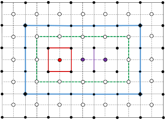
Figure 1: The two-dimensional lattice for the gauge theory (shown with solid lines) and the dual lattice for the scalar theory (shown with broken lines). Under duality, the electric operator along the solid violet link is mapped to the difference of $\phi$’s at the two violet vertices and the Wilson loop along the boundary of the plaquette shown in solid red is mapped to $\pi$ at the centre of the plaquette shown in red. The blue rectangle encloses the region $R$, with the four atypical boundary points at the edges shown as diamonds. The green rectangle encloses the dual region $\tilde{R}$.

For simplicity, we start with the case of the $U(1)$ gauge theory in $2+1$ dimensions. We take the spatial lattice to be square. The degrees of freedom are link variables $\theta_{l}$ valued in $U(1)$. The gauge invariant observables are electric operators, $E_{l}$, which are conjugate to the link variables and Wilson loop operators, which are defined for a plaquette and given by $\exp(\mathrm{i}\sum_{l}\theta_{l})$, where the sum is over oriented links along the boundary of the plaquette. We will be interested in the entanglement of a rectangular region $R$ shown in Fig 1. The electric centre arises when we keep all gauge invariant operators in $R$ in the algebra and corresponds to specifying the normal component of the electric field for each boundary point. For the four atypical boundary points where more than one boundary edge meet, the sum of the electric fields along the two boundary edges meeting at the point lie in the centre. By Gauss’ law, this is equivalent to specifying the centre element by the value of the sum of the electric fields along the outward directed links emanating from the boundary point. The magnetic centre is obtained after one deletes all the electric link operators for the boundary links from the algebra. It is easy to easy that the resulting algebra now has only one operator in the resulting magnetic centre which corresponds to the Wilson loop along the boundary of the region.

The dual lattice is obtained by replacing each link of the original lattice with a dual link, in the standard fashion as shown in Fig 1. This exchanges points of the original lattice with an elementary plaquette in the dual which surrounds the point and vice-versa. The dual theory lives on the dual lattice and is that of a free scalar. The gauge invariant operators discussed above map as follows. The Wilson loop along an elementary plaquette surrounding the point $i$ in the dual is

$$W=\pi(i),$$ (37)

where $\pi(i)$ is the operator which is the conjugate momentum for the scalar operator located at vertex $i$, $\phi(i)$. The electric field along link $l$ is

$$E_{l}\leftrightarrow\Delta\phi=\phi(i+1)-\phi(i),$$ (38)

where $\phi(i)$ denotes the value of the scalar at site $i$ and $\phi(i+1)$ at the site $i+1$ which is displaced by one lattice unit orthogonal to the direction of the link $l$. See Fig.1.

The algebra of observables for the region of interest in the scalar case includes all operators $\phi(i),\pi(i)$ with $i\in{\tilde{R}}$ where ${\tilde{R}}$ is the dual region shown in Fig 1. It is easy to see that this maps to the magnetic centre for the gauge theory with one small difference. The operator $\sum_{i}\phi(i)$, with the sum being over all points in ${\tilde{R}}$, is absent in the gauge theory case. Its absence gives rise to a non-trivial centre which, as per the discussion above for the magnetic centre, is given by the Wilson loop which measures the total magnetic flux threading $R$. This operator is dual to $\sum_{i\in{\tilde{R}}}\pi(i)$. Once the operator $\sum_{i\in{\tilde{R}}}\phi(i)$ is also present in the algebra, the centre becomes trivial.

Despite this difference, the entanglement of ground state is the same in the two algebras, as long as the theory is on a finite lattice. The reason is that the scalar theory has a global shift symmetry

$$\phi(i)\to\phi(i)+\alpha,$$ (39)

generated by the total conjugate momentum

$$\Pi^{T}=\sum_{i\in L}\pi(i).$$ (40)

On a finite lattice, this symmetry is not spontaneously broken, and the ground state is an eigenstate of $\Pi^{T}$ with zero total momentum.

Since we can write $\Pi^{T}$ as a sum of total inside and outside conjugate momenta,

$$\Pi^{T}=\Pi_{\mathrm{in}}^{T}+\Pi_{\mathrm{out}}^{T},$$ (41)

the reduced density matrix must commute with $\Pi_{\mathrm{in}}^{T}$ and therefore must be block-diagonal in any eigenbasis of $\Pi_{\mathrm{in}}^{T}$. Because of this, the reduced density matrix does not change when the operator $\sum_{i\in\tilde{R}}\phi(i)$, which is conjugate to $\Pi_{\mathrm{in}}^{T}$, is deleted from the algebra. This means that the reduced density matrix, and therefore the entanglement spectrum, is the same as that of the magnetic centre algebra which is the algebra of the region without the operator $\sum_{i\in\tilde{R}}\phi(i)$ whose removal makes no difference.

Let us end with a few comments. First, the argument above showing that the density matrices of the two algebras which differ by the inclusion of the operator $\sum_{i\in{\tilde{R}}}\phi(i)$ are the same will be true in any eigenstate of the total momentum, $\Pi^{T}$. In contrast, the argument will not apply for an infinite lattice since the global shift symmetry is spontaneously broken in this case and the ground state is no longer an eigenstate of $\Pi^{T}$.

Second, it was found in Donnelly:2016mlc that, for theories on compact manifolds, the EHS entanglement for the gauge theory agrees with the scalar entanglement (with a suitable identification of the UV regulator). The EHS entanglement includes a non-extractable piece which scales like the boundary area and diverges in the continuum limit. In contrast, for the scalar, the full result for the entanglement is, of course, extractable. As a result, the extractable entanglement in the two cases will not agree. Let us emphasise that this is not a contradiction since we are comparing two different algebras and the operations which can be carried out during quantum distillation or dilution depend on the operators at one’s disposal. It is nonetheless interesting that the full entanglement does agree in the two cases. We also note that the scalar case and the magnetic centre only differ by one operator, as noted above, and this difference is not expected to give rise to a differing area law contribution for the magnetic centre and scalar cases.

Also, we have not been careful about the distinction between the compact and non-compact $U(1)$ theories above. It is well known that the compact $U(1)$ theory maps to a compact boson (see, for example, Agon:2013iva for a careful discussion). The momenta $\pi(i)$ are well defined operators in the compact case, but instead of the field $\phi(i)$ we can work with the phase $e^{\mathrm{i}\phi}$ which is well defined (for $\phi$ having periodicity $2\pi$). The duality map can then be easily worked out and the discussion above can be extended in a precise manner for the compact case as well.

3.2 Gauge Field in $3+1$ Dimensions

Let us next consider a $U(1)$ gauge theory in $3+1$ dimensions. Its dual is also a $U(1)$ gauge theory. Under duality, the electric and magnetic fields are exchanged with each other,

$$\mathbf{E} \to\mathbf{B},$$ (42)

$$\mathbf{B} \to-\mathbf{E}.$$

The Gauss law and the Bianchi identity are exchanged under this map. On the lattice, the magnetic field actually refers to the value of the Wilson loop around an elementary plaquette, and the electric field to the corresponding electric operator on a link. Under duality, links are exchanged with plaquettes on the dual lattice and this exchanges the electric link and Wilson loop operators, in a lattice version of eq.(42). The electric field operators and the Wilson loop operators constitute a complete set of gauge invariant observables. In our subsequent discussion, we will sometimes be a little loose and refer to the electric link operators and Wilson loop operators on the lattice as electric and magnetic fields.

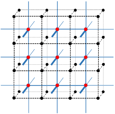
Figure 2: A boundary face in the three dimensional case. Wilson loops that lie in the magnetic centre are shown as dashed lines on the boundary face. Their duals are electric link operators along the outward directed normals, shown as blue links emanating from the vertices of the dual lattice denoted in red.

The electric centre is obtained when we keep all the gauge invariant operators in the region of interest in the algebra. Due to the Gauss law constraint, the centre elements can be thought of as corresponding to the normal component of the electric field on the boundary.

The magnetic centre is obtained, as in the $2+1$-dimensional case, by removing all electric link operators on the boundary from the algebra. The resulting algebra then has as its centre the Wilson loop operators along all the plaquettes that lie on the boundary faces. Under duality, these are exchanged with electric link operators. For the region $R$ of interest in the original theory, we can define a dual core region ${\tilde{R}}$ obtained by displacing all boundary lattice points half a lattice unit inwards along the normal. The electric link operators dual to the Wilson loops in the magnetic centre of the original theory lie along links which go from the boundary points of ${\tilde{R}}$ outwards along the normal direction. In Fig 2, we show one boundary face and the plaquette operators in the original lattice which are in the magnetic centre and lie on this face along with their dual electric link operators.

The dual description of the magnetic centre case can therefore be thought of as follows. We augment the set of all gauge invariant operators in the region ${\tilde{R}}$ with the additional electric link operators along links which extend from boundary points outward along the normal. This extended algebra then has the additional electric operators as its centre. For a typical boundary point of ${\tilde{R}}$, where no boundary faces meet, this additional electric operator is related to the other electric link operators emanating from the boundary point, which are already present in the algebra, by the Gauss law constraint. Therefore, the addition of this operator to the algebra actually does not change it. However, for boundary points where more than one face meet the additional electric link operators added in this way do enlarge the algebra, since Gauss’ law only relates the sum of these outgoing electric link operators to the electric link operators already present in ${\tilde{R}}$.

In this way, we see that the magnetic centre case in the original theory is related to the electric centre case in the dual theory by the addition of some additional electric link operators, which in the continuum limit we expect to be the same as the electric centre case. Conversely, the electric centre case of the original theory, with the addition of some extra electric link operators at boundary points where more than one face meet, maps to the magnetic centre case of the dual theory.

We end with the following comment. In the continuum limit, an alternative is to just choose a different latticisation where the boundary does not have ‘corners;’ for example, if the boundary is a sphere, we can choose the links in the lattice to consist of radial lines and, at a particular radius, latitudes and longitudes of the sphere. While this lattice is extremely odd at the origin, the main point is that in this lattice the electric centre exactly dualises to the magnetic centre, thereby tying in with the expectation that the additional operators discussed above will not make a significant difference in the continuum limit.

3.3 $p$-Form Theory in $d+1$ Dimensions

It is now easy to generalise the discussion for the general case of a $p$-form gauge potential in $d+1$ dimensions. This is dual to a $(d-p-1)$-form potential theory. We denote the components of the potential by $B_{\mu_{1}\mu_{2}\cdots\mu_{p}}$ and the field strength by $H_{\mu_{1}\mu_{2}\cdots\mu_{p+1}}$ and those of the dual potential and dual field strength by ${\tilde{B}}_{\mu_{1}\mu_{2}\cdots\mu_{d-p-1}}$ and ${\tilde{H}}_{\mu_{1}\mu_{2}\cdots\mu_{d-p}}$ respectively. On the spatial lattice, the gauge invariant observables are the electric fields $H_{0i_{1}i_{2}\cdots i_{p}}$ which are defined on a $p$-dimensional hypercube, and the magnetic fields are given by the oriented sum of $H_{i_{1}i_{2}\cdots i_{p+1}}$ along all the faces of a $(p+1)$-dimensional hypercube. The Gauss law constraint in the lattice takes the following form: Consider all $p$-dimensional hypercubes which share a vertex. Then the sum of all electric fields which share $p-1$ directions in common on these hypercubes must vanish. The Bianchi identity is given as follows. Consider a $(p+2)$-dimensional hypercube which has $(p+1)$-dimensional hypercubes as its faces. Then the oriented sum of the magnetic fields along all these faces vanishes. The Gauss law constraint and the Bianchi identity are exchanged under duality.

For a region $R$ which is now a $d$-dimensional hypercube, the boundary faces are $(d-1)$-dimensional. The outward normal component of the electric field at a boundary point corresponds to hypercubes which have one link extending from the boundary point along the outward normal and the remaining $p-1$ links along the $d-1$ directions tangent to the boundary. The electric centre case arises when all gauge invariant operators present in $R$ are included in the algebra. Using Gauss’ law, the centre can then be thought of as the outward normal component of the electric field at all boundary points. The magnetic centre is obtained by removing all electric operators which take values on hypercubes that lie along the boundary. It consists of all the magnetic field operators which take values on $(p+1)$-dimensional hypercubes lying on the boundary.

Consider now the magnetic centre in the dual theory. The dual core region ${\tilde{R}}$ is as above given by the region in the dual lattice obtained by going half a lattice unit inwards from the boundary of $R$ along the normal. The magnetic centre operators of the $p$-form theory map to outward normal components of the electric field at the boundary points of ${\tilde{R}}$ in the dual theory. Under the duality map, these operators are added to all the gauge invariant operators in ${\tilde{R}}$ to give the full algebra. Using Gauss’ law, as in the case of the $U(1)$ theory in $3+1$ dimensions above, the additional operators actually only arise from boundary points of ${\tilde{R}}$ where more than one faces meet.

The one exception which needs to be handled separately is the case of a $(d-1)$-form gauge potential in $d+1$ dimensions. This is analogous to case of a gauge theory in $2+1$ dimensions, discussed above. Here the dual theory is that of a scalar, and the magnetic centre case of the original theory maps to the situation where all operators in the scalar theory lying in the dual core region are included in the algebra, with the exception of $\sum_{i\in{\tilde{R}}}\phi(i)$. The centre has one element which in the total magnetic flux in $R$ or in dual description the total momentum in ${\tilde{R}}$, $\sum_{i\in{\tilde{R}}}\pi(i)$. Including the operator $\sum_{i\in{\tilde{R}}}\phi(i)$ gives rise to a trivial centre. Using an argument analogous to that in §3.1, it follows that the addition of this operator does not change the density matrix and the entanglement entropy for a state which has a fixed value of the total momentum, $\sum_{i\in{\tilde{L}}}\pi(i)$.

4 Conclusions

In this paper, we have analysed some aspects pertaining to the entanglement entropy for gauge theories. We argued that for the extended Hilbert space definition, or equivalently the electric centre case, with entanglement entropy given in eq.(1), the probability to be in the different superselection sectors, $p_{i}$, is determined by the two-point function of the normal component of the electric field along the boundary – more specifically, eq.(10) in the Abelian and eq.(28) in the non-Abelian cases. We find that the two-point function is dominated by modes which carry high momenta in the direction normal to the boundary. These modes give rise to a UV divergent contribution to the two-point function. As a result, in the continuum limit, the contribution from the first two terms in eq.(1) will drop out from the mutual information of two disjoint regions and the relative entropy between two states which have only finite energy excitations about the vacuum.

It is worth noting that our conclusions also apply to theories with matter. Strictly speaking, we assume that the theories are weakly coupled at short distances. In the non-Abelian case this would be true for asymptotically free theories. Our conclusions could be altered if the UV behaviour is different, from example if the behaviour is governed by a fixed point which changes the anomalous dimensions of the electric field operators sufficiently from the free field case. We also note that in the Abelian case, the high momentum modes give rise to a logarithmic divergence in the two-point function of the normal component of the electric field, this divergence is universally present irrespective of dimension.

Let us also mention that the behaviour of $2+1$-dimensional Maxwell theory has been studied numerically, Casini:2014aia . It was found that the the dependence on the centre does indeed drop out in the continuum limit. It was also argued quite generally using the expectation that the relative entropy and mutual information for “thin regions” should vanish in the continuum limit that the contribution of the classical term to the relative entropy or the mutual information would drop out in this limit Casini:2013rba . Some evidence for this was also obtained numerically, Casini:2014aia . Our analysis confirms these expectations.

In the more general case of an Abelian $p$-form gauge potential theory in $d+1$ spacetime dimensions, we find that the corresponding probability distribution is determined by the Laplacian for a $(p-1)$-form living on the $(d-1)$-dimensional spatial boundary of the region of interest. The high momentum modes dominate the behaviour of the relevant two-point function in this more general case as well and give rise to a similar logarithmic divergence in the two-point function. As a result, the classical term in the entanglement, $-\sum_{i}p_{i}\log p_{i}$, drops out in the continuum limit from the mutual information and the relative entropy which only receive a contribution from the quantum piece in the entanglement entropy. We have not been very careful about studying the zero modes of the $(p-1)$-form theory. See Donnelly:2016mlc for an important discussion in this regard; see also the comments at the end of §2.1, where we discuss how in Maxwell theory the zero modes can sometimes lead to contributions in the mutual information or relative entropy arising from the classical term.

Finally, we have also briefly studied some aspects of electric-magnetic duality on the lattice. We find that the magnetic centre for a $p$-form in $d+1$ dimensions maps to the electric centre case for the dual $(d-p-1)$-form, with the addition of a few more operators to the algebra. In the continuum limit, these extra operators will not make a difference while computing the mutual information or the relative entropy and the electric and magnetic theories will therefore agree in the results we obtain for these quantities.

It will be worth extending our discussion for gravity in the linearised limit. For some existing discussion, see Donnelly:2016auv ; Speranza:2017gxd ; Geiller:2017whh ; Camps:2018wjf . The classical term can be thought of as arising due to gauge transformations with support on the boundary of the region of interest. Elucidating the nature of these boundary degrees of freedom in the gravity case in more detail, and the resulting classical term, both for a planar boundary with a Rindler horizon, and at asymptotic null infinity would be quite interesting. It would also be interesting to explore how these considerations might be related to proposals for soft hair on a black hole horizon, Hawking:2016msc ; Hawking:2016sgy ; Haco:2018ske .

- (1) P. V. Buividovich and M. I. Polikarpov, Entanglement entropy in gauge theories and the holographic principle for electric strings, Phys. Lett. B670 (2008) 141 [0806.3376].
- (2) W. Donnelly, Decomposition of entanglement entropy in lattice gauge theory, Phys. Rev. D85 (2012) 085004 [1109.0036].
- (3) S. Ghosh, R. M. Soni and S. P. Trivedi, On The Entanglement Entropy For Gauge Theories, JHEP 09 (2015) 069 [1501.02593].
- (4) S. Aoki, T. Iritani, M. Nozaki, T. Numasawa, N. Shiba and H. Tasaki, On the definition of entanglement entropy in lattice gauge theories, JHEP 06 (2015) 187 [1502.04267].
- (5) R. M. Soni and S. P. Trivedi, Entanglement entropy in (3 + 1)-d free U(1) gauge theory, JHEP 02 (2017) 101 [1608.00353].
- (6) H. Casini, M. Huerta and J. A. Rosabal, Remarks on entanglement entropy for gauge fields, Phys. Rev. D89 (2014) 085012 [1312.1183].
- (7) R. M. Soni and S. P. Trivedi, Aspects of Entanglement Entropy for Gauge Theories, JHEP 01 (2016) 136 [1510.07455].
- (8) K. Van Acoleyen, N. Bultinck, J. Haegeman, M. Marien, V. B. Scholz and F. Verstraete, The entanglement of distillation for gauge theories, Phys. Rev. Lett. 117 (2016) 131602 [1511.04369].
- (9) M. Ohya and D. Petz, Quantum entropy and its use. Springer Science & Business Media, 2004.
- (10) E. Witten, APS Medal for Exceptional Achievement in Research: Invited article on entanglement properties of quantum field theory, Rev. Mod. Phys. 90 (2018) 045003 [1803.04993].
- (11) C. Eling, Y. Oz and S. Theisen, Entanglement and Thermal Entropy of Gauge Fields, JHEP 11 (2013) 019 [1308.4964].
- (12) K.-W. Huang, Central Charge and Entangled Gauge Fields, Phys. Rev. D92 (2015) 025010 [1412.2730].
- (13) W. Donnelly and A. C. Wall, Entanglement entropy of electromagnetic edge modes, Phys. Rev. Lett. 114 (2015) 111603 [1412.1895].
- (14) W. Donnelly and A. C. Wall, Geometric entropy and edge modes of the electromagnetic field, Phys. Rev. D94 (2016) 104053 [1506.05792].
- (15) F. Zuo, A note on electromagnetic edge modes, 1601.06910.
- (16) W. Donnelly, B. Michel and A. Wall, Electromagnetic Duality and Entanglement Anomalies, Phys. Rev. D96 (2017) 045008 [1611.05920].
- (17) J. S. Dowker, Renyi entropy and for p-forms on even spheres, 1706.04574.
- (18) A. Gromov and R. A. Santos, Entanglement Entropy in 2D Non-abelian Pure Gauge Theory, Phys. Lett. B737 (2014) 60 [1403.5035].
- (19) Đ. Radičević, Notes on Entanglement in Abelian Gauge Theories, 1404.1391.
- (20) W. Donnelly, Entanglement entropy and nonabelian gauge symmetry, Class. Quant. Grav. 31 (2014) 214003 [1406.7304].
- (21) H. Casini and M. Huerta, Entanglement entropy for a Maxwell field: Numerical calculation on a two dimensional lattice, Phys. Rev. D90 (2014) 105013 [1406.2991].
- (22) L.-Y. Hung and Y. Wan, Revisiting Entanglement Entropy of Lattice Gauge Theories, JHEP 04 (2015) 122 [1501.04389].
- (23) Đ. Radičević, Entanglement in Weakly Coupled Lattice Gauge Theories, JHEP 04 (2016) 163 [1509.08478].
- (24) C.-T. Ma, Entanglement with Centers, JHEP 01 (2016) 070 [1511.02671].
- (25) E. Itou, K. Nagata, Y. Nakagawa, A. Nakamura and V. I. Zakharov, Entanglement in Four-Dimensional SU(3) Gauge Theory, PTEP 2016 (2016) 061B01 [1512.01334].
- (26) H. Casini and M. Huerta, Entanglement entropy of a Maxwell field on the sphere, Phys. Rev. D93 (2016) 105031 [1512.06182].
- (27) Đ. Radičević, Entanglement Entropy and Duality, JHEP 11 (2016) 130 [1605.09396].
- (28) M. Nozaki and N. Watamura, Quantum Entanglement of Locally Excited States in Maxwell Theory, JHEP 12 (2016) 069 [1606.07076].
- (29) S. Aoki, E. Itou and K. Nagata, Entanglement entropy for pure gauge theories in 1 + 1 dimensions using the lattice regularization, Int. J. Mod. Phys. A31 (2016) 1650192 [1608.08727].
- (30) V. Balasubramanian, A. Bernamonti, B. Craps, T. De Jonckheere and F. Galli, Entwinement in discretely gauged theories, JHEP 12 (2016) 094 [1609.03991].
- (31) A. Agarwal, D. Karabali and V. P. Nair, Gauge-invariant Variables and Entanglement Entropy, Phys. Rev. D96 (2017) 125008 [1701.00014].
- (32) S. Aoki, N. Iizuka, K. Tamaoka and T. Yokoya, Entanglement Entropy for 2D Gauge Theories with Matters, Phys. Rev. D96 (2017) 045020 [1705.01549].
- (33) M. Hategan, Entanglement Entropy in Pure Gauge Lattices, 1705.10474.
- (34) Z. Yang and L.-Y. Hung, Gauge choices and entanglement entropy of two dimensional lattice gauge fields, JHEP 03 (2018) 073 [1710.09528].
- (35) M. Pretko, On the Entanglement Entropy of Maxwell Theory: A Condensed Matter Perspective, 1801.01158.
- (36) A. Blommaert, T. G. Mertens, H. Verschelde and V. I. Zakharov, Edge State Quantization: Vector Fields in Rindler, JHEP 08 (2018) 196 [1801.09910].
- (37) M. Hategan, Entanglement entropy in lattice theories with Abelian gauge groups, Phys. Rev. D98 (2018) 045020 [1809.00230].
- (38) M. M. Anber and B. J. Kolligs, Entanglement entropy, dualities, and deconfinement in gauge theories, JHEP 08 (2018) 175 [1804.01956].
- (39) A. Blommaert, T. G. Mertens and H. Verschelde, Edge Dynamics from the Path Integral: Maxwell and Yang-Mills, 1804.07585.
- (40) J. Lin and Đ. Radičević, Comments on Defining Entanglement Entropy, 1808.05939.
- (41) M. Huerta and L. A. Pedraza, Numerical determination of the entanglement entropy for a Maxwell field in the cylinder, 1808.01864.
- (42) A. M. Polyakov, Compact Gauge Fields and the Infrared Catastrophe, Phys. Lett. B59 (1975) 82.
- (43) S. Ghosh and S. Raju, Quantum information measures for restricted sets of observables, Phys. Rev. D98 (2018) 046005 [1712.09365].
- (44) J. B. Kogut and L. Susskind, Hamiltonian Formulation of Wilson’s Lattice Gauge Theories, Phys. Rev. D11 (1975) 395.
- (45) Đ. Radičević, Spin Structures and Exact Dualities in Low Dimensions, 1809.07757.
- (46) M. Campiglia, L. Freidel, F. Hopfmüller and R. M. Soni, Scalar Asymptotic Charges and Dual Large Gauge Transformations, 1810.04213.
- (47) C. A. Agón, M. Headrick, D. L. Jafferis and S. Kasko, Disk entanglement entropy for a Maxwell field, Phys. Rev. D89 (2014) 025018 [1310.4886].
- (48) W. Donnelly and L. Freidel, Local subsystems in gauge theory and gravity, JHEP 09 (2016) 102 [1601.04744].
- (49) A. J. Speranza, Local phase space and edge modes for diffeomorphism-invariant theories, JHEP 02 (2018) 021 [1706.05061].
- (50) M. Geiller, Lorentz-diffeomorphism edge modes in 3d gravity, JHEP 02 (2018) 029 [1712.05269].
- (51) J. Camps, Superselection Sectors of Gravitational Subregions, 1810.01802.
- (52) S. W. Hawking, M. J. Perry and A. Strominger, Soft Hair on Black Holes, Phys. Rev. Lett. 116 (2016) 231301 [1601.00921].
- (53) S. W. Hawking, M. J. Perry and A. Strominger, Superrotation Charge and Supertranslation Hair on Black Holes, JHEP 05 (2017) 161 [1611.09175].
- (54) S. Haco, S. W. Hawking, M. J. Perry and A. Strominger, Black Hole Entropy and Soft Hair, 1810.01847.