Dark Energy Survey Year 1 Results: Constraints on Intrinsic Alignments and their Colour Dependence from Galaxy Clustering and Weak Lensing

Abstract

We perform a joint analysis of intrinsic alignments and cosmology using tomographic weak lensing, galaxy clustering and galaxy-galaxy lensing measurements from Year 1 (Y1) of the Dark Energy Survey. We define early- and late-type subsamples, which are found to pass a series of systematics tests, including for spurious photometric redshift error and point spread function correlations. We analyse these split data alongside the fiducial mixed Y1 sample using a range of intrinsic alignment models. In a fiducial Nonlinear Alignment Model (NLA) analysis, assuming a flat $\Lambda$CDM cosmology, we find a significant difference in intrinsic alignment amplitude, with early-type galaxies favouring $A_{\mathrm{IA}}=2.38^{+0.32}_{-0.31}$ and late-type galaxies consistent with no intrinsic alignments at $0.05^{+0.10}_{-0.09}$. The analysis is repeated using a number of extended model spaces, including a physically motivated model that includes both tidal torquing and tidal alignment mechanisms. In multiprobe likelihood chains in which cosmology, intrinsic alignments in both galaxy samples and all other relevant systematics are varied simultaneously, we find the tidal alignment and tidal torquing parts of the intrinsic alignment signal have amplitudes $A_{1}=2.66^{+0.67}_{-0.66}$, $A_{2}=-2.94^{+1.94}_{-1.83}$, respectively, for early-type galaxies and $A_{1}=0.62^{+0.41}_{-0.41}$, $A_{2}=-2.26^{+1.30}_{-1.16}$ for late-type galaxies. In the full (mixed) Y1 sample the best constraints are $A_{1}=0.70^{+0.41}_{-0.38}$, $A_{2}=-1.36^{+1.08}_{-1.41}$. For all galaxy splits and IA models considered, we report cosmological parameter constraints consistent with the results of the main DES Y1 cosmic shear and multiprobe cosmology papers.

1 Introduction

Within a little over a decade the study of late-time cosmology has grown from a set of theoretically justified but empirically untested ideas, to a rigorous experimental field. With the current generation of surveys now in the process of cataloguing millions of galaxies and new experiments planned to reach even larger cosmological volumes, the ideas of the past half century are now finally being implemented. In many ways low redshift measurements are complementary to other cosmological probes such as the Cosmic Microwave Background (CMB), the masses and abundances of galaxy clusters and cosmographic observables such as supernovae and strong lensing. Cosmological lensing probes the large scale distribution of mass directly and is also sensitive to geometric distance ratios, which define a window of sensitivity on the line of sight (see e.g. Weinberg et al. 2013).

Advances have come in part due to the sheer number of galaxies imaged by modern surveys. Since shape noise scales as the inverse root of the number of galaxies, expanding datasets have afforded gradually better signal-to-noise on cosmic shear statistics. Though statistical power can be continuously improved, an additional floor to the precision of the resulting cosmological inferences is imposed by systematic errors. In order to codify this, it is typically necessary to introduce “nuisance parameters” in any cosmological analysis, which are marginalised out. In the systematics-limited regime the only way to achieve tighter cosmological constraints is to improve one’s understanding of the systematics in question. One is left with a choice of acquiring information from external data or theory, and incorporating it into the analysis via a prior, or self-calibrating the systematics by including new measurements in the likelihood calculation.

Indeed, there has long been recognition that combining different measurements can improve the quality of cosmological constraints. Even very similar measurements extracted from the same galaxy survey can be complementary if their parameter degeneracies and their systematic errors differ. Combining lensing auto-correlations with galaxy-galaxy lensing and two-point galaxy clustering, for example, is powerful as a means to “self-calibrate” redshift error and other systematic uncertainties (see e.g. Joachimi & Bridle 2010). Another idea is to use cross correlations between lensing and CMB maps as a way to check for residual errors in the shape measurement process (Schaan et al., 2017; Mishra-Sharma et al., 2018; Harnois-Déraps et al., 2017; Abbott et al., 2018).

There are many possible sources of systematic uncertainty in late-time datasets (see Mandelbaum 2017, 2015 for cosmic shear-specific reviews and Ross et al. 2011; Mandelbaum et al. 2013; Leistedt et al. 2016; Kwan et al. 2017; Prat et al. 2017 [their Section V]; Elvin-Poole et al. 2017 for more detailed discussions of systematics that can occur in galaxy-galaxy lensing and galaxy clustering measurements). One major class of systematics arises from local astrophysical effects, which can mimic a cosmological shear signal. Spurious (non-cosmological) correlations between galaxies, known as intrinsic alignments (IAs) have long been known to affect cosmic shear estimates. Such effects arise because galaxies are not independent point measurements of the large scale cosmic shear field, but rather extended astrophysical objects that interact with each other and with their environment. It was realised over a decade ago that galaxies hosted by a common dark matter halo tend to align through shared tidal interactions (Catelan et al., 2001) and rotational torquing (Mackey et al., 2002). This results in alignment in the intrinsic shapes of physically close pairs of galaxies, known as II correlations. An often more pervasive effect comes from the fact that the same foreground matter experiences local gravitational interactions over short spatial scales, and also induces lensing of background galaxies. This generates correlations in shape between foreground galaxies and background sources (Hirata & Seljak, 2004), which are known as the GI contribution; this is often the dominant form of intrinsic alignments in lensing surveys. It has been shown by Croft & Metzler (2000) and others that the total IA contamination to cosmological shear can be as high as $10\%$ in modern surveys, and neglecting these effects can result in significant cosmological biases (Kirk et al., 2012; Krause et al., 2016).

The particular challenge posed by IA modelling is in large part down to the nature of the contamination; biases in shear measurement, photo-$z$ estimation, point spread function (PSF) modelling errors and instrumental systematics are all fundamentally methodological problems. One can understand them using image simulations and mitigate them by devising new methods. In contrast, IA correlations are a real astrophysical signal, which enters much the same angular scales as cosmic shear itself. Indeed, it has been suggested that if correctly modelled they can in principle be used as a probe of cosmology (Chisari & Dvorkin, 2013; Troxel & Ishak, 2015), primordial non-Gaussianity (Chisari et al., 2016), or galaxy formation (Schmitz et al., 2018). Given this context, if we are to avoid becoming limited by intrinsic alignments it is important that the lensing community develops a robust understanding of the nature of this signal and techniques for dealing with it. A number of mitigation techniques have been proposed, involving discarding physically close pairs of galaxies (Catelan et al., 2001; Kirk et al., 2015), downweighting (King & Schneider, 2003; Heymans & Heavens, 2003; Heavens, 2003; Heymans et al., 2005), or nulling (Joachimi & Schneider, 2010). All of these methods depend on the existence of accurate redshift information to allow galaxies to be located relative to each other along the line of sight. Significantly, they are also ineffective in mitigating GI correlations, which are often dominant in galaxy samples typical of cosmic shear measurements. Alternatively one could impose colour or morphology cuts designed to isolate a subsample free of IA contamination (Krause et al., 2016). This approach, however, has a number of obvious drawbacks, not least that one has no theoretical grounds for believing any given population of galaxies to be perfectly without intrinsic alignments.

The issues with modelling IAs can broadly be separated into two problems. First, the models are known to perform poorly on small physical scales, where intra-halo interactions dominate the galaxy two-point correlations. Progress on these scales requires an understanding of how galaxies populate and interact within their host halos (see, for example, Schneider & Bridle 2010 for a halo model-based treatment of the small scale IA power spectra). Halo models have the advantage of mathematical elegance, and can be (validly) extended down to nonlinear scales. They do, however, require calibration using numerical simulations, and are thus only as reliable as the simulations in question. A similar idea is to use “semi-analytic” modelling, based on cosmological simulations, as discussed in Joachimi et al. (2013). Model testing on these scales is further complicated by the influence of other poorly understood effects such as baryonic feedback. The second problem is the existence of known deficiencies in IA modelling on two-halo scales. These occur primarily because the most common large scale alignment models are based on a population of galaxies that is highly unrepresentative of the typical samples used for lensing studies. Recent years have seen the emergence of a small handful of more complete physically motivated models, which seek to build a unified IA prescription in a mixed galaxy population (Blazek et al. 2015; Tugendhat & Schäfer 2017; Blazek et al. 2017; see also Dark Energy Survey Collaboration 2016; Troxel et al. 2017 for practical implementations). Similarly, Larsen & Challinor (2016) use perturbation theory to model scale dependence of CMB - intrinsic shape cross correlations, which they argue should match the GI term in cosmic shear on large scales. They predict that IAs due to tidal torquing should exhibit a very similar scale dependence to the commonly used linear alignment model.

It has been noted in both simulations and data that the choice of galaxy shape estimation method can alter the magnitude of the IA signal by an overall scale-independent factor (Singh & Mandelbaum, 2016; Hilbert et al., 2017). One interesting idea devised by Leonard & Mandelbaum (2018) takes advantage of this concept, using multiple shape measurement techniques to measure the scale dependence of the IA signal in the nonlinear regime, a subject that is poorly understood at a theoretical level at the present time. This method carries the advantage of being relatively robust to photometric redshift error compared with conventional measurements.

Notably several authors have found the intrinsic alignment correlations measured in hydrodynamic simulations to be dependent on galaxy type, mass and magnitude; these dependencies are also poorly understood at the theoretical level (Joachimi et al., 2013; Chisari et al., 2015; Hilbert et al., 2017). In recent years there have been attempts to place observational constraints on the alignment properties of galaxy samples more representative of the sort used for cosmological lensing measurements (Mandelbaum et al., 2011; Blazek et al., 2012; Tonegawa et al., 2017). Despite these efforts, given limitations in the sample selection and size, we still have little clear information about the expected values of the free parameters in our IA models. It is thus common to choose what is known to be an incomplete model and to marginalise over it using uninformative priors.

This work sits alongside a series of other DES studies based on the same data. Zuntz et al. (2017) describe the construction of the Y1 shape catalogues and provide a basic usage guide. In Prat et al. (2017) and Elvin-Poole et al. (2017) the galaxy-galaxy lensing and galaxy clustering measurements and their potential systematics are examined in detail. The cosmological analysis choices and the robustness of the Y1 pipeline to various forms of systematic error are tested using noiseless synthetic data in Krause et al. (2017) and N-body simulations in MacCrann et al. (2018). Cosmology constraints from cosmic shear alone and shear, galaxy-galaxy lensing and clustering are set out in Troxel et al. (2017) and Dark Energy Survey Collaboration (2017) respectively. More recent follow-on work has included a methodology paper for a future analysis combining $3\times 2$pt measurements with CMB cross-correlations (Baxter et al., 2018), a joint constraint on the local Hubble parameter using DES alongside external Baryon Acoustic Oscillation and Big Bang Nucleosynthesis data (Dark Energy Survey Collaboration, 2018b) and, most recently, a study setting out a series of cosmological modelling extensions (Dark Energy Survey Collaboration, 2018a). This paper seeks to explore a significant cosmological systematic using the same Y1 lensing dataset: intrinsic alignments and their colour dependence.

In Section 2 we outline the theory of modelling intrinsic alignments and introduce the formalism adopted in this study. We describe the DES Y1 data in Section 3 and define a number of galaxy samples, which are selected to separate differences in the underlying IA signal. Section 4 sets out the measurements used in this work, which include real space two-point correlations of cosmic shear, galaxy-galaxy lensing and galaxy clustering. In Section 5 we present the main results of this analysis, using a range of intrinsic alignment models and three different galaxy samples. We conclude and provide a brief summary in Section 6.

2 Theory & Background

2.1 Observational Constraints on Intrinsic Alignments

Attempts to constrain intrinsic shape correlations between galaxies fall broadly into two categories. The first are direct constraints, which typically use galaxies at low to intermediate redshift and often impose colour cuts to isolate well-measured red galaxies, and assume some fixed known cosmology. Correlation statistics used in these measurements are explicitly designed to maximise the IA signal (e.g. Hirata et al. 2007, Faltenbacher et al. 2009, Okumura & Jing 2009, Mandelbaum et al. 2011, Blazek et al. 2011, Blazek et al. 2012). Since IA correlations are a fundamentally local phenomenon it is common to focus on samples for which high quality spectroscopic data is available, allowing three-dimensional reconstruction of the physical field. In such studies it is also common to restrict measurements to the low redshift regime, where the amplitude of cosmological lensing is low.

The second class of measurements are indirect, or simultaneous constraints. Generally they measure statistics designed to be sensitive to cosmic shear such as $\xi_{\pm}$ and use faint high-redshift galaxies in which the cosmological signal is strongest. While some studies attempt to remove the lensing signal to obtain a clearer picture of IAs (e.g. Blazek et al. 2012; Chisari et al. 2014), cosmic shear and galaxy-galaxy lensing analyses must necessarily address the questions of intrinsic alignments and lensing together. Any investigation that involves marginalising over IAs rather than suppressing them directly falls into this category (Heymans et al., 2013; Dark Energy Survey Collaboration, 2016; Jee et al., 2016; Hildebrandt et al., 2017; Köhlinger et al., 2017; Troxel et al., 2017; Chang et al., 2018; Hikage et al., 2018). The assumptions about IAs differ slightly between studies, but they all assume the same basic model (the nonlinear alignment model), sometimes with a multiplicative scaling in redshift or luminosity.

There is some direct evidence for differences in the IA contamination, depending on the nature of the galaxy sample Heymans et al. (2013); Troxel et al. (2017). Broadly there are two paradigms: early-type ellipticals, which tend to be redder and structurally pressure dominated; and late-type spirals, which tend to be bluer and rotation dominated. The former are thought to align through tidal interactions with the background large scale structure of the Universe. If a dark matter halo sits in a local gradient in the gravitational field, it will be sheared along that gradient and nearby galaxies will become aligned with their common background tidal field. If the distortion is small, the induced ellipticity can be assumed to be linear in the gravitational potential. A handful of direct studies over the past decade have sought to place constraints on IAs in red galaxies (see e.g. Mandelbaum et al. 2006; Hirata et al. 2007; Okumura & Jing 2009; Joachimi et al. 2011; Li et al. 2013; Singh et al. 2015). In each case, a strong IA signal is reported, with no statistically significant detection of redshift dependence.

The picture for late-type galaxies is rather different. These objects form galactic discs, which, depending on the orientation, will have an apparent ellipticity. One common picture is that galaxy spin (which ultimately decides the disc orientation) is generated by tidal torquing, exerted on a halo in its early stages of development. Direct constraints on blue galaxy IAs are generally relatively weak. Measurements have been made on blue samples from SDSS (York et al., 2000) and WiggleZ (Parkinson et al., 2012) at low to mid redshifts, but impose only upper limits on the intrinsic alignment amplitude (Hirata et al., 2007; Mandelbaum et al., 2011). Blazek et al. (2012) use a blue sample from SDSS to make such a measurement, but place an upper limit only on the IA signal at $z\sim 0.1$. A similar analysis by Tonegawa et al. (2017), using Emission Line Galaxies from FastSound and the Canada France Hawaii Lensing Survey (CFHTLenS), also reports a null detection, showing no evidence of either non-zero amplitude or redshift dependence.

For a more detailed overview of the theory and observational history of intrinsic alignments we direct the reader to a number of extensive reviews on the subject (Troxel & Ishak, 2015; Joachimi et al., 2015; Kirk et al., 2015; Kiessling et al., 2015)

2.2 Theory

Theory modelling and parameter estimation for this study are performed within the CosmoSIS framework (Zuntz et al., 2015). We use the Multinest nested sampling package (Feroz et al., 2013) to sample the joint model space of cosmology, intrinsic alignment and systematics parameters. For consistency with previous publications, our choices regarding sampler settings follow those used by Krause et al. (2017). The dark matter power spectrum is estimated at each cosmology using camb , with nonlinear corrections generated by Halofit (Takahashi et al., 2012). We do not explicitly model baryonic effects and the intrinsic alignment prescriptions considered do not attempt to model the one-halo regime, but as noted in the next section our choice of scale cuts is relatively conservative. Except in Section 5.3.4, where we explicitly set out to extend the cosmological model space, we assume a flat $\Lambda$CDM cosmology with six free parameters $\mathbf{p}_{\mathrm{cosmology}}=(h,\Omega_{\mathrm{m}},\Omega_{\mathrm{b}},A_{\mathrm{s}},n_{\mathrm{s}},\Omega_{\nu}h^{2})$.

The following paragraphs describe how each of the three types of observable correlation, and their intrinsic alignment contribution, is modelled for the purposes of parameter inference.

2.2.1 Cosmic Shear

For cosmic shear we use real-space angular correlation functions in four tomographic bins. The measurements map onto the angular shear power spectrum via Hankel transforms:

$$\xi^{ij}_{\pm}(\theta)=\frac{1}{2\pi}\int\ell J_{0/4}(\ell\theta)C_{\gamma\gamma}^{ij}(\ell)d\ell$$ (1)

where the indices $ij$ indicate a pair of tomographic bins, and $J_{0}$ and $J_{4}$ are Bessel functions of the first kind. For the moment we will assume no intrinsic alignments, and so the shear-shear angular power spectrum $C_{\gamma\gamma}$ is interchangeable with the signal predicted from cosmological lensing only $C_{\mathrm{GG}}$. $C_{\mathrm{GG}}$ is related to the dark matter power spectrum under the Limber approximation as,

$$C^{ij}_{\mathrm{GG}}=\int^{\chi_{\mathrm{hor}}}_{0}\frac{g^{i}(\chi)g^{j}(\chi)}{\chi^{2}}P_{\delta}\left(k=\frac{\ell}{\chi},z\right)d\chi.$$ (2)

We assume a flat universe, such that the transverse angular diameter distance $S_{K}(\chi)=\chi$. The term $\chi_{\mathrm{hor}}$ is the comoving horizon distance and the lensing kernel in each bin is given by

$$g^{i}(\chi)=\frac{3}{2}\frac{H^{2}_{0}\Omega_{\mathrm{m}}}{c^{2}}\frac{\chi}{a(\chi)}\int^{\chi_{\mathrm{hor}}}_{\chi}n^{i}(\chi^{\prime})\frac{\chi^{\prime}-\chi}{\chi^{\prime}}d\chi^{\prime}$$ (3)

The redshift distributions $n(z)$ are assumed to be normalised over the depth of the survey, and defined such that $n(z)dz=n(\chi)d\chi$. Likelihoods for trial cosmologies are calculated by generating theory angular spectra, which are integrated over with the Bessel kernels, resampled at the appropriate angular scales, and then compared with the measurements of $\xi_{\pm}^{ij}$.

2.2.2 Galaxy Clustering

The formalism for predicting galaxy clustering observables follows by close analogy to the previous section. The spatial distribution of lens galaxies traces out the underlying dark matter, albeit via some unknown galaxy bias. In this work we adopt a simple scale-independent linear bias model, with the overdensity of galaxies at a particular scale related to the dark matter density as $\delta_{g}(k)=b_{g}(z)\delta(k)$. We adopt the same scale cuts used in the DES Y1 key paper (Dark Energy Survey Collaboration, 2017), under which it has been demonstrated that higher-order bias terms have negligible impact on cosmology (Krause et al., 2017). The correlation function of galaxy density has the form

$$w^{ij}(\theta)=\frac{1}{2\pi}\int\ell J_{0}(\ell\theta)C_{\delta_{g}\delta_{g}}^{ij}(\ell)d\ell,$$ (4)

where the galaxy-galaxy angular power spectrum between tomographic bins $i$ and $j$ is given by

$$C^{ij}_{\delta_{g}\delta_{g}}(\ell)=\int^{\chi_{\mathrm{hor}}}_{0}\frac{n_{l}^{i}(\chi)n_{l}^{j}(\chi)}{\chi^{2}}b_{g}^{i}b_{g}^{j}P_{\delta}\left(k=\frac{\ell}{\chi},z\right)d\chi.$$ (5)

Since we have no good first-principles model for the galaxy bias and its redshift evolution we allow $b_{g}^{i}$ to vary independently in each redshift bin. Within each bin $b_{g}^{i}$ is scale and redshift independent and can thus be taken outside of the integral. The subscript $l$ in the $n_{l}^{i}(\chi)$ terms denotes lens galaxies, for which we use the DES Y1 redMaGiC sample as presented by Elvin-Poole et al. (2017).

2.2.3 Galaxy-Galaxy Lensing

The final part of the $3\times 2$pt combination of late-time probes is galaxy-galaxy lensing. As the cross correlation between galaxy shapes and number density, the galaxy-galaxy lensing formalism follows similar lines to the two auto-correlations described above. A commonly used observable, $\gamma_{t}(\theta)$, is given by the Hankel transform

$$\gamma^{ij}_{t}(\theta)=\frac{1}{2\pi}\int\ell J_{2}(\ell\theta)C_{\delta_{g}\gamma}^{ij}(\ell)d\ell,$$ (6)

where the angular spectrum (again assuming zero IAs for the moment) is

$$C^{ij}_{\delta_{g}\mathrm{G}}(\ell)=\int^{\chi_{\mathrm{hor}}}_{0}\frac{n_{l}^{i}(\chi)g^{j}(\chi)}{\chi^{2}}b_{g}^{i}P_{\delta}\left(k=\frac{\ell}{\chi},z\right)d\chi.$$ (7)

Again, we assume linear galaxy bias, allowing the $\delta_{g}\mathrm{G}$ power spectrum to be expressed as the matter power spectrum modulated by a scale-independent bias coefficient $b_{g}^{i}$. The lensing kernel $g(\chi)$ is defined by equation 3. It is worth bearing in mind that a small handful of different galaxy-galaxy lensing estimators exist in the literature, most notably $\Delta\Sigma$ (related to $\gamma_{t}$ via a factor of the critical density $\Sigma_{\mathrm{c}}$; see Mandelbaum et al. 2013) and $\Upsilon$ (devised to remove contributions from small scales; see Baldauf et al. 2010).

2.2.4 Modelling Intrinsic Alignments

Even a perfectly unbiased measurement of the ellipticity-ellipticity two-point function in a set of galaxies is not a pure estimate of the cosmic shear spectrum. Correlations between the intrinsic (pre-shear) shapes contribute unknown additive terms of the form

$$C^{ij}_{\gamma\gamma}(\ell)=C^{ij}_{\mathrm{GG}}(\ell)+C^{ij}_{\mathrm{II}}(\ell)+C^{ij}_{\mathrm{GI}}(\ell)+C^{ji}_{\mathrm{GI}}(\ell),$$ (8)

where we make the distinction between the observable estimate for the shear correlation $C_{\gamma\gamma}$ and the cosmological GG component. Note that it is $\gamma\gamma$, not GG that appears in equation 1. The spectra with subscripts GI and II are intrinsic alignment correlations, and arise via the mechanisms described in Section 1. The IA contribution to galaxy-galaxy lensing follows a similar form, but is insensitive to II correlations:

$$C^{ij}_{\delta_{g}\gamma}(\ell)=C^{ij}_{\delta_{g}\mathrm{G}}(\ell)+C^{ij}_{\delta_{g}\mathrm{I}}(\ell),$$ (9)

A number of different prescriptions for calculating the GI and II terms exist in the literature.

These Limber projections in bins $ij$ are simply expressed in terms of the IA power spectra in the form

$$C^{ij}_{\mathrm{II}}(\ell)=\int\frac{n^{i}(\chi)n^{j}(\chi)}{\chi^{2}}P_{\mathrm{II}}\left(k=\frac{\ell}{\chi},\chi\right)d\chi$$ (10)

and

$$C^{ij}_{\mathrm{GI}}(\ell)=\int\frac{g^{i}(\chi)n^{j}(\chi)}{\chi^{2}}P_{\mathrm{GI}}\left(k=\frac{\ell}{\chi},\chi\right)d\chi,$$ (11)

where the GI and II power spectra $P_{\mathrm{GI}}$ and $P_{\mathrm{II}}$ are generic, and can be generated by any of the IA models discussed below. Similarly, the galaxy-intrinsic term, which appears in galaxy-galaxy lensing correlations is given by:

$$C^{ij}_{\delta_{g}\mathrm{I}}(\ell)=\int\frac{n_{l}^{i}(\chi)n^{j}(\chi)}{\chi^{2}}b^{i}_{g}P_{\mathrm{GI}}\left(k=\frac{\ell}{\chi},\chi\right)d\chi,$$ (12)

under the assumption of linear galaxy bias. Note that though they are both sensitive to the GI power spectrum $P_{\mathrm{GI}}$, the relation between $C_{\mathrm{GI}}$ and $C_{\delta_{g}\mathrm{I}}$ is non-trivial because the projection kernels in equations 11 and 12 differ.

Under the common family of “tidal alignment” models, in which the intrinsic galaxy shapes are assumed to be linearly related to the local tidal field, the IA power spectra are assumed to be of the same shape as the matter power spectrum, but subject to a redshift-dependent rescaling:

$$P_{\mathrm{GI}}(k,z)=A(z)P_{\delta}(k,z),$$ (13)

and

$$P_{\mathrm{II}}(k,z)=A^{2}(z)P_{\delta}(k,z).$$ (14)

Owing to its good performance in matching data and simulations, one prescription, known as the nonlinear alignment (NLA) model (Bridle & King, 2007) has become particularly popular. This is an empirical modification to the linear alignment model of Catelan et al. (2001) and Hirata & Seljak (2004), whereby the linear matter power spectrum is replaced by the nonlinear spectrum. The normalisation in the NLA model is typically expressed as

$$A(z)=-A_{\mathrm{IA}}\bar{C_{1}}\frac{3H^{2}_{0}\Omega_{\mathrm{m}}}{8\pi G}D^{-1}(z)\left(\frac{1+z}{1+z_{0}}\right)^{\eta_{\mathrm{IA}}}.$$ (15)

The dimensionless amplitude $A_{\mathrm{IA}}$ is an unknown scaling parameter governing the strength of the IA contamination for a particular sample of galaxies, and is generally left as a free parameter to be constrained. Here $G$ is the gravitational constant and $D(z)$ is the linear growth factor. The normalisation constant $\bar{C_{1}}$ is typically fixed at a value obtained from the SuperCOSMOS Sky Survey by Brown et al. (2002) of $\bar{C_{1}}=5\times 10^{-14}M_{\odot}^{-1}h^{-2}$ Mpc³. The redshift evolution is expressed by a power law index $\eta_{\mathrm{IA}}$, which has been measured in low redshift samples of luminous red galaxies (Joachimi et al., 2011). The value of $\eta_{\mathrm{IA}}$ can capture underlying evolution of the alignment or evolution within a given sample of other galaxy properties that impact alignment, such as luminosity and morphology. The denominator $1+z_{0}$ sets a pivot redshift, for which we assume $z_{0}=0.62$ whenever equation 15 is used in this paper. Note that the same value was used in the previous Y1 analyses of Troxel et al. (2017) and Dark Energy Survey Collaboration (2017).

In addition to the baseline NLA model, one could conceivably add flexibility to the IA model by allowing the amplitudes entering the GI and II power spectra (equations 13 and 14) to behave as independent free parameters. For the purpose of this study, we will treat this as a separate IA model with four free parameters (the fourth row of Table 1). Alternatively, one could maintain the link between the II and GI spectra, and instead allow $A$ to vary independently in each redshift bin. This approach, analogous to the treatment of galaxy bias in this paper, has four free parameters and is referred to as the ‘Flexible NLA’ model (row 3 of Table 1).

The NLA model, defined by the equations above, is physically motivated and found to match observational data well in specific circumstances. That is, on linear scales, in bright red low-redshift populations where intrinsic alignments have been measured with high signal-to-noise (Hirata et al., 2007; Blazek et al., 2011). Unfortunately, there is neither prima facie theoretical motivation nor strong observational evidence to suggest this model applies equally well to the type of galaxies sampled by modern lensing surveys. Moreover, the picture is further complicated by the fact that galaxies used for lensing cosmology are typically mixed (i.e. with no explicit colour or morphology based cuts), going from a predominantly elliptical population at low redshifts to one dominated by rotation-dominated spirals at high $z$. There is evidence from both theoretical studies (Catelan et al., 2001; Mackey et al., 2002) and from hydrodynamic simulations (Chisari et al., 2015; Hilbert et al., 2017) that the alignment mechanisms at play in these different galaxy types are very different.

The standard approach to this question is to assume that red galaxies can be modelled using the NLA model and blue galaxies have no intrinsic shape correlations. In this picture the observed IA contribution in cosmic shear data is a pure NLA signal, but scaled by an effective IA amplitude, which absorbs the dilution due to randomly oriented blue galaxies. This strategy will, however, be effective only in the limit of zero alignments in blue galaxies.

In addition to the NLA model, we will also employ a model intended to address this concern. Based on perturbation theory, the model of Blazek et al. (2017) combines alignment contributions from tidal torquing (quadratic in the tidal field; thought to dominate in blue galaxies) and from tidal alignments (linear in the tidal field; dominant in red galaxies). In this model, the intrinsic galaxy shape $\gamma_{ij}^{I}$ can be expressed as an expansion in the tidal field $s_{ij}$ and the density field $\delta$, with the subscripts denoting components of spin-2 tensor quantities.

$$\gamma_{ij}^{I}=C_{1}s_{ij}+C_{2}\left(s_{ik}s_{kj}-\frac{1}{3}s^{2}\right)+C_{1\delta}\left(\delta s_{ij}\right)+\cdots$$ (16)

In this expansion, $C_{1}$ captures the tidal alignment contribution. Using the full nonlinear density field to calculate $s_{ij}$ yields the NLA model. $C_{2}$ captures the quadratic contribution from tidal torquing. Finally, $C_{1\delta}$ can be seen as a contribution from “density weighting” the tidal alignment contribution: we only observe IAs where there are galaxies, which contributes this additional term at next-to-leading order. While these coefficients can be associated with tidal alignment and tidal torquing mechanisms, as done here, these can also be considered “effective” parameters capturing any relevant astrophysical processes that produce IA with the given dependence on cosmological fields. Furthermore, we note that $A_{1}\neq 0$ can potentially arise from tidal torquing combined with nonlinear structure growth (Larsen & Challinor, 2016; Blazek et al., 2017). Despite this potential complication, in the following discussion we assume the standard mapping between these parameters and the underlying IA formation mechanisms.

As implemented in this work, this formalism has four adjustable parameters: an amplitude and a redshift power law governing each of the tidal alignment ($C_{1}$) and tidal torque ($C_{2}$) power spectra. Following Blazek et al. (2017), we assume $C_{1\delta}=b^{\mathrm{src}}_{g}C_{1}$, i.e. the density weighting is given by the bias of the source sample. The source bias can be then either be fixed (as in Troxel et al. 2017, which assumed $b^{\mathrm{src}}_{g}=1$), or marginalised over a plausible range of values. For the main section of this paper we fix source bias. Note that the model requires no explicit assumptions about the fraction of red galaxies or its evolution with redshift. We have the following parameterization:

$$C_{1}(z)=-A_{1}\bar{C_{1}}\rho_{\mathrm{crit}}\frac{\Omega_{\mathrm{m}}}{D(z)}\left(\frac{1+z}{1+z_{0}}\right)^{\eta_{1}}$$ (17)

for the tidal alignment part. For the tidal torque contribution,

$$C_{2}(z)=5A_{2}\bar{C_{1}}\rho_{\mathrm{crit}}\frac{\Omega_{\mathrm{m}}}{D^{2}(z)}\left(\frac{1+z}{1+z_{0}}\right)^{\eta_{2}},$$ (18)

with the four IA parameters $\mathbf{p_{\mathrm{IA}}}=(A_{1},\eta_{1},A_{2},\eta_{2})$.

The corresponding IA power spectra (GI and II) are $k$-dependent functions derived from perturbation theory and are given by integrals over the matter power spectrum; for the full expressions and visual comparison see Blazek et al. (2017) Sections A-C. These alignment power spectra define what we will refer to as the ‘Complete TATT’ model. We will also treat the pure tidal alignment and tidal torque scenarios as models in their own right (Table 1, third and fourth from last rows).

In the most naïve theoretical picture of intrinsic alignments, galaxies are either pressure-supported ellipticals, whose shapes respond linearly to the background tidal field, or rotation-dominated spirals, whose alignment is quadratic in the tidal field. For comparison with previous theoretical studies we will, then, consider TA and TT cases, with power spectra obtained from the equations above, but with fixed amplitudes $A_{2}=0$ and $A_{1}=0$ respectively.

For computational reasons we assume negligible B-mode IA contribution. These analysis choices have been tested and shown to have no significant effect on our conclusions in Appendix A and Appendix B.

The $k$ dependent terms in these equations are computed using the FAST-PT code (McEwen et al., 2016; Fang et al., 2017). For both the mode-coupling integrals and the TATT model predictions, we use code implementations within CosmoSIS, which are common to Troxel et al. 2017 and the forecasts in Blazek et al. 2017.

The intrinsic alignment models discussed in the above paragraphs and their free parameters are summarised in Table 1. For reference we also include the ranges over which the various parameters are allowed to vary. The prescription referred to as the ‘Complete TATT Model’ in this work, which includes $C_{1}$ and $C_{2}$ contributions and has fixed $b^{\mathrm{src}}_{g}=1$ is identical to the ‘Mixed Model’ of Troxel et al. 2017, the ‘Complete Model’ (Section D) of Blazek et al. 2017 and the ‘TATT Model’ of Dark Energy Survey Collaboration 2018a. It is worth noting that Troxel et al. 2017 also present constraints with the baseline and flexible NLA models, but with cosmic shear alone. Both Troxel et al. (2017) and Dark Energy Survey Collaboration (2017) opt to marginalise over the two-parameter NLA model as their fiducial IA treatment; their headline cosmology constraints come from such treatment.

IA Model	Free Parameters	Priors
No Alignments	None	None
NLA (fiducial)	$A_{\mathrm{IA}}$	$U[-6,6]$
NLA (fiducial)	$\eta_{\mathrm{IA}}$	$U[-5,5]$
Flexible NLA	$A^{(i)},i\in(1,2,3,4)$	$U[-6,6]$
NLA (separate GI $+$ II)	$A_{\mathrm{GI}},A_{\mathrm{II}}$	$U[-6,6]$
	$\eta_{\mathrm{GI}},\eta_{\mathrm{II}}$	$U[-5,5]$
Tidal Alignment	$A_{1}$	$U[-6,6]$
Tidal Torque	$A_{2}$	$U[-6,6]$
TATT	$A_{1}$	$U[-32,32]$
	$A_{2}$	$U[-6,6]$
TATT ($z$ power law)	$A_{1}$	$U[-32,32]$
	$A_{2}$	$U[-6,6]$
	$\eta_{1},\eta_{2}$	$U[-32,32]$

Table 1: Summary of the intrinsic alignment models used in this paper. The right-hand column shows the parameters varied under each model. In principle the galaxy bias in the source population $b_{g}^{\mathrm{src}}$ also enters the TATT model (both variants) and the TA models (Blazek et al., 2017) . Other than in Appendix A, where we explicitly test its impact, however, we fix $b_{g}^{\mathrm{src}}=1$.

2.2.5 Other Systematics

In addition to five cosmological parameters and the IA model parameters we marginalise over thirteen nuisance parameters. The point here is to encapsulate residual systematic errors entering the measurement due to a number of effects. Following Dark Energy Survey Collaboration (2017), we marginalise over an offset in the mean of the photometric redshift distributions in each of the four lensing bins. At least in the context of $3\times 2$pt cosmology at current precision there is evidence in the literature that a shift in the ensemble mean of the redshift distribution is the most salient form of redshift error (see e.g. Figure 20 of Dark Energy Survey Collaboration 2017). This transforms the $n(z)$ entering into equation 3 as $n^{i}(z)\rightarrow n^{i}(z-\Delta z^{i})$, where $\Delta z^{i}$ is the redshift error for bin $i$. There is reason for caution here, however, particularly if one wishes to draw conclusions about less well-understood effects such as intrinsic alignments: photo-$z$ modelling errors can easily be absorbed into an apparent IA signal (see, for example, Section 6.6 of Hildebrandt et al. 2017). We seek to test the impact of photo-$z$ modelling insufficiency in Section 5.2 and find our results are robust to reasonable changes in the shape of the $n(z)$s. In addition, there is some level of uncertainty in the treatment of shear estimation bias, for which it is necessary to include an additional nuisance parameter $m^{i}$ per source bin. This modulates the angular spectra in equations 1 and 6 by factors of $(1+m^{i})(1+m^{j})$ and $(1+m^{i})$ respectively. Finally, there are five nuisance parameters to account for lens redshift errors and five for lens galaxy bias. The redshift parameters act in the same way as the source errors, but on the clustering sample $n_{l}(z)$. Our treatment of lens bias is discussed in Section 2.2.2.

Since the clustering sample is unchanged relative to that set out in Dark Energy Survey Collaboration (2017) we adopt the priors on lens redshift error and galaxy bias used in that paper. Similarly, the uncertainty in $m^{i}$ is dominated by limitations in how the shear measurement handles blending. This is not expected to differ significantly with galaxy type, and so for all of the samples described in the next section we adopt the fiducial Gaussian prior on $m^{i}$ recommended by Zuntz et al. (2017). The source redshift error, however, could very easily differ between galaxy samples of different colour. We recompute priors on $\Delta z^{i}$ for the different samples using galaxies from the COSMOS field, a calculation discussed further in Section 3.4.

3 Data & Sample Selection

In this section we define the galaxy samples used in this paper. The subsamples are disjoint populations from the DES Y1 weak lensing catalogue, intended to isolate morphological differences relevant to IA. The following paragraphs discuss the practical details of the split, including how we manage selection effects.

3.1 The Dark Energy Survey Y1 Data

The Dark Energy Survey (DES) has now completed its five-year observing campaign, covering a footprint of around 5000 square degrees to a depth of $r\sim 24.1$ magnitudes. The observing program made use of the 570 megapixel DECam (Flaugher et al., 2015), which is mounted on the Victor Blanco telescope at the Cerro Tololo Inter-American Observatory (CTIO) in northern Chile. Its five-band grizY photometry spans a broad region of the optical and near infrared spectrum between 0.40 and 1.06 microns. Each $griz$ exposure is 90 seconds in duration and the final mean tiling depth will be ten exposures over the full footprint.

The wide-field observations for Y1 encompass a large region completely overlapping the footprint of the South Pole Telescope (SPT; Carlstrom et al. 2011) CMB experiment and extends roughly over the range $\delta=[-60,-40]$ degrees. A significantly smaller region in the north of the Y1 footprint also overlaps with the Stripe 82 field of the Sloan Digital Sky Survey (SDSS); data from this region are excluded from this analysis, as they were from the main Y1 cosmology papers. In total the Y1 cosmology dataset encompasses an area of 1321 square degrees of the southern sky with a mean depth of three exposures. This includes masking for potentially bad regions deemed to be of unsuitable quality for cosmological inference. A more detailed description of the final Gold sample can be found in Drlica-Wagner et al. (2018). These data were collected between 31st August 2013 and 9th February 2014 during the first full season of DES operations.

For lensing measurements we make use of the larger of the two DES Y1 shape catalogues (see Zuntz et al. 2017), which contains $\sim 26$ million galaxies in the final cosmology selection. This dataset, known as the metacalibration catalogue, relies on the eponymous technique for correcting shear measurement bias. We discuss how these corrections, which include sample selection effects, are computed in Section 4.

The catalogue used for two-point clustering measurements comprises a set of luminous red galaxies selected by the redMaGiC algorithm (Rozo et al., 2016) using a method designed to minimise photometric redshift error. The sample contains roughly 0.66 M galaxies at constant comoving density over the range $z=0.15-0.9$ (Elvin-Poole et al., 2017).

3.2 Blinding

This analysis was doubly blinded, following the same protocol outlined in Zuntz et al. (2017) and implemented in Troxel et al. (2017). First, the early stages of this analysis were performed using modified shear catalogues, wherein each measured ellipticity was multiplied by a blinding factor. The factor was constructed such that the mathematical bounds of the ellipticity were unchanged by the transformation. This catalogue-level blinding was maintained until shortly after the point at which the fiducial Y1 results (Dark Energy Survey Collaboration, 2017) were unblinded. By this time the basic methodology of the analysis had been decided and the selection criteria for the galaxy samples were fixed.

Second, higher level blinding was imposed by the authors throughout the course of this analysis. The axis labels and range of any figures showing cosmological parameter constraints were omitted during the blinded period. This was intended to prevent unconcious bias from entering the analysis, for example, if the split samples were seen to be exhibit significant tensions. The bulk of the analysis, including running chains, comparing constraints from colour samples and creating figures, and all basic methodological decisions was carried out prior to lifting either form of blinding. A small number of notable changes were made after unblinding, namely: (a) generating and validating the multicolour covariance matrix, (b) running and analysing the chains shown in Figure 16. Though this could conceivably lead to expectation bias. We do, however, carry out a series of validation tests, which involve comparing subsections of the new covariance matrix (and the derived constraints) with the single colour matrices used in the earlier sections of this paper. The cosmology contours in Figure 17 were also generated only after the multicolour covariance matrix had been finalised. These steps, while not comprehensive, guard to some extent against such bias.

3.3 Splitting the Y1 Shape Catalogue

There are a number of terms used in the literature to classify galaxies, which are broadly analogous but non-identical. This paper primarily focuses on two, both of which are ultimately derived from differences in the flux of a galaxy in different optical bands. Though these names are often used somewhat interchangeably in the literature, in the following analysis the terms ‘early-type’, ‘red’, ‘late-type’ and ‘blue’ have distinct meanings, as set out below. The characteristics of these samples are summarised in Table 2. In both cases, we use these flux-based categories as a proxy for galaxy morphology and kinematics, which affect which alignment mechanism(s) are most relevant.

3.3.1 Spectral Class

A quantity commonly used to split galaxy populations is spectral class. Template-based photo-$z$ codes such as bpz  work by redshifting a library of spectral templates repeatedly. Fits are performed to produce a likelihood as a function of redshift for each galaxy, assuming each of the discrete library templates. The conditional likelihoods are interpolated to produce a single $p(z)$ and a non-integer best-fitting spectral class $T_{\mathrm{BPZ}}$, which represents an interpolated blend of templates and acts as a morphological class for each galaxy. This quantity has been used in previous studies to divide galaxies expected to have different systematics (Simon et al., 2013; Heymans et al., 2013). We follow those papers and define a boundary at $T_{\mathrm{BPZ}}=1$ to separate “early-type” and “late-type” galaxies. Imposing this split on the DES Y1 cosmology sample of Troxel et al. (2017), we obtain early- and late-type samples containing 4.8 M and 28.8 M galaxies respectively. In Figure 1 we show the distributions of photometric colour, defined by the difference in magnitudes between the $r$ and $z$ bands, and $r$-band magnitude in these two populations.

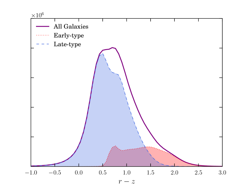
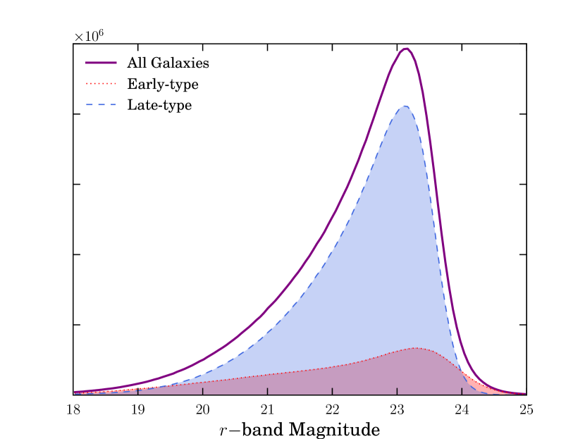
Figure 1: Top: The one dimensional distribution of photometric $r-z$ colour in the samples described in this study. The solid purple line shows the histogram of the full sample, and the dashed blue and dotted red lines show late-type and early-type galaxies only. Bottom: $r$-band magnitude distributions of the galaxy samples defined in this paper. Note that the solid purple line here is defined by the metacalibration selection flag, and corresponds to the dark red histogram in Figure 3 of Zuntz et al. (2017).

3.3.2 Photometric Colour

Another quantity frequently used as a proxy for morphological type is photometric colour, defined by differences between the measured brightness of a galaxy in different bands. The 2D histogram of galaxies in colour magnitude space is expected to be bimodal (Wyder et al., 2007). In the following we use a boundary in the $r-z$ plane to define red and blue galaxies, defined by the equation

$$r-z=a^{i}_{\mathrm{rz}}\times r+b^{i}_{\mathrm{rz}}.$$ (19)

Unlike previous studies, we do not have reliable $k$-corrected magnitudes, nor do we impose selection criteria designed to produce a homogenous low-redshift sample. To account for the fact that the observed colour-magnitude diagram is redshift dependent we adjust the values of the parameters $a_{\mathrm{rz}}$ and $b_{\mathrm{rz}}$ in each tomographic bin (denoted by the index $i$). The boundary is shifted manually in each bin to roughly follow the green valley division between peaks, and is shown in Figure 2. In the four DES Y1 source redshift bins we obtain $\mathbf{a}_{\mathrm{rz}}=(0.04,0.12,0.05,0.00)$ and $\mathbf{b}_{\mathrm{rz}}=(-0.1,-1.7,0.15,1.6)$.

It is worth finally bearing in mind that there are several similar sets of photometric measurements derived from DES Y1, which are used by different authors in slightly different contexts. In summary, three useful sets of galaxy fluxes are available to us: (a) those obtained from the source detection algorithm SExtractor, (b) the best-fitting fluxes from running our shape measurement code (known as metacalibration; see Section 4.1.1) on the raw galaxy images, (c) those obtained using metacalibration from reprocessed images with neighbour light subtracted away, using a technique called Multi-Object Fitting (MOF). Though (a) are included in the Gold catalogue, they are not used in this work. We use type (b) photometry, and products derived thereof, for the catalogue splits described in this section as well as for dividing galaxies into redshift bins. Though MOF partially mitigates the effects of blending and so is thought to produce more accurate fluxes, type (c) fluxes are used only for estimating the galaxy redshift PDFs (see Section 3.4 below). This detail arises from an oddity of DES Y1: for computational reasons, at the time of writing only one MOF shape run was carried out. To allow us to split on (c) type photometry and correctly treat the selection effects induced, we would require additional MOF runs on several sets of artificially sheared images (see Section 4.1.1).

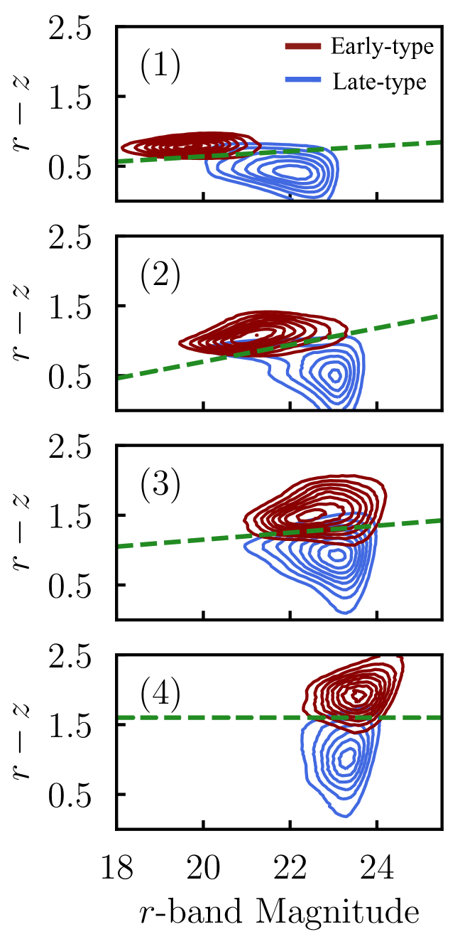
Figure 2: The distribution of galaxies in $r-z$ colour-magnitude space in the Y1 metacalibration catalogue. The panels show galaxies in four tomographic bins, which are labelled in parentheses. The red contours indicate early-type $(T_{\mathrm{BPZ}}<1)$ objects only, and the blue contours are the equivalent for late-type galaxies. Each is independently normalised to unity. The green dashed line shows the divisions used to define the red and blue samples described in Section 3.3, and are placed such that they roughly mimic the split between the red and blue contours.

Sample	$N_{\mathrm{gal}}$	$z^{\mathrm{med}}$	$\bar{r}$	$r-z$
All galaxies	25.7 M	0.57	22.2	0.79
Early	4.8 M	0.65	21.9	1.31
Late	20.8 M	0.55	22.3	0.64
Red	6.5 M	0.61	21.8	1.25
Blue	19.2 M	0.55	22.4	0.64
Early $\cap$ Red	2.3 M	0.66	21.9	1.37
Late $\cap$ Blue	18.5 M	0.55	22.4	0.62

Table 2: Observational characteristics of the sub-populations defined in this paper. Note that the mean and median values shown are weighted by the mean galaxy response $R=(R_{11}+R_{22})/2$.

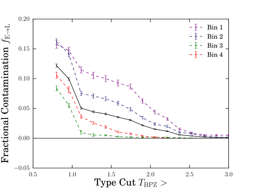
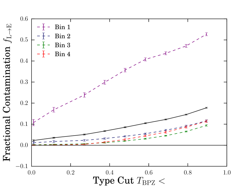
Figure 3: Galaxy colour leakage as a function of the upper/lower cut imposed on $T_{\mathrm{BPZ}}$. The upper panel shows the magnitude of misclassified early-type galaxies that appear in our late-type sample. The lower panel shows the equivalent late-type to early-type contamination. The leakage estimator $f_{\mathrm{Type1\rightarrow Type2}}$ here is defined as the fraction of the lensing weight in each bin coming from such misclassified galaxies. In each case we show the four tomographic bins, as well as the whole unbinned sample in black.

Finally we attempt to gauge the level of leakage between our galaxy samples. Since we define our samples about fixed boundary in noisy measured quantities it is inevitable that there will be some cross-contamination. That is, a population of galaxies that, if measured under ideal noiseless conditions would be classified as one type, but which in reality end up being classified as the other. We test this as follows. We re-run the bpz algorithm twice on a matched COSMOS sample (described in Section 3.4), (a) using a set of degraded galaxy fluxes designed to mimic DES-like noise levels and (b) using the original fluxes measured with DECam from deeper observations than in the DES wide-field. This exercise provides a redshift PDF and a best-estimate $T_{\mathrm{BPZ}}$ value per COSMOS galaxy. We then define an early-type sample based on the noisy $T_{\mathrm{BPZ}}$ from run (a) and compute the fraction of the lensing weight in that sample that is contributed by galaxies where the value from run (b) is $T_{\mathrm{BPZ}}>1$. The results are shown in Figure 3.

The leakage is relatively small in most tomographic bins, with the mis-allocated lensing weight at or below $\sim 15\%$. The notable exception is the lowest tomographic bin in the early-type sample, which exhibits a strong fractional contamination. This can be rationalised in simple terms, as follows; there is some degeneracy between colour and redshift. That is, galaxies assigned to the red sample and the lowest redshift bin can be (a) inherently red, low redshift galaxies or (b) bluer objects, which have been redshifted and thus appear red. A similar logic applies, such that a fraction of the blue sample galaxies in the upper tomographic bin will actually be inherently red low redshift objects mistakenly identified. The key difference is that the quality of the photo-$z$ for the red low $z$ objects tends to be superior than for more distant galaxies. The leakage of blue galaxies into the lowest bin is thus stronger than the converse. The significance of this feature for our results is tested by rerunning a subset of the chains in Section 5.1 with the lowest redshift bin removed. As discussed in that section, the omission of the high-leakage bin does not produce a significant shift in either the favoured cosmology, nor the best-fitting IA parameters.

3.4 Photometric Redshifts

We derive estimates for the redshift distribution of our samples using the bpz code (Benítez, 2000). The results have been tested using simulations, against a limited spectroscopic sample and against an alternative redshift algorithm (Hoyle et al., 2017). For each sample used in this study, the per-galaxy PDFs are stacked in four tomographic bins with bounds $z=[0.2,0.43,0.63,0.9,1.3]$. Galaxies are assigned to bins using the expectation value of the $p(z)$ estimated with metacalibration photometry. The run of bpz on the more optimal MOF photometry then provides the $p(z)$ stacked to generate the ensemble $n(z)$ estimates. We show the measured $n(z)$ obtained using bpz for $T_{\mathrm{BPZ}}<1$ and $T_{\mathrm{BPZ}}>1$ galaxies in Figure 4.

The main shear selection defined by Zuntz et al. (2017) has been subjected to a rigorous set of tests designed to constrain this redshift bias (Hoyle et al., 2017; Davis et al., 2017; Gatti et al., 2018). This information is incorporated into cosmic shear analyses via (non-zero centred) priors on redshift nuisance parameters. Unfortunately, one cannot guarantee that these priors will be robust to arbitrary division of the data. If we propose to use any subset of the catalogue for tomographic shear measurements, it is necessary to re-derive appropriate photo-$z$ priors. To do this we use galaxies from the partially overlapping COSMOS field. The low-noise 32-band photometry provides high-quality point redshift estimates for these galaxies. In the following we will take these as “true” redshifts. In principle we can test for bias in a particular sample by comparing the distribution of the COSMOS redshifts to the ensemble redshift distribution estimates for the same set of galaxies in the DES images. Selecting the galaxies in the COSMOS overlap, however, can itself induce selection effects, since the COSMOS galaxies are somewhat unrepresentative of DES in magnitude, colour and size. The COSMOS catalogue is thus resampled such that the resulting sample matches the DES Y1 data. The process results in a set of 200,000 DES galaxies matched to COSMOS counterparts with similar flux in four bands $griz$ and size (see Hoyle et al. 2017 for a full description of the algorithm).

We divide these galaxies into four tomographic bins according to mean redshift, as estimated from a re-run of bpz on the artificially noisy COSMOS $griz$ metacalibration fluxes. In each bin we compute a weighted mean

$$\left<z\right>^{(i)}=\frac{\sum^{N^{(i)}_{\mathrm{gal}}}_{j=1}w_{j}z^{\mathrm{C}}_{j}}{\sum^{N^{(i)}_{\mathrm{gal}}}_{j=1}w_{j}},$$ (20)

where $z^{\mathrm{C}}_{j}$ is the COSMOS redshift estimate for galaxy $j$ and the sum runs over all galaxies placed in redshift bin $i$. The weight is $w_{j}$ is given by the mean response (averaged over the two ellipticity components; see Section 4).

The offset between the mean COSMOS redshift and the equivalent weighted mean using the bpz Monte Carlo samples from artificially noisy MOF photometry provides a constraint on the level of systematic bias in the latter. We derive $\delta z$ in this way for our early, late and full samples, as defined by $T_{\mathrm{BPZ}}$. The result is shown in Table 3.

Selection	$\delta z^{(1)}$	$\delta z^{(2)}$	$\delta z^{(3)}$	$\delta z^{(4)}$
All Galaxies	$-0.006\pm 0.018$	$-0.014\pm 0.018$	$0.018\pm 0.017$	$-0.018\pm 0.018$
Early-Type	$-0.022\pm 0.020$	$-0.040\pm 0.012$	$-0.008\pm 0.012$	$-0.044\pm 0.014$
Late-Type	$-0.003\pm 0.020$	$-0.007\pm 0.023$	$0.030\pm 0.020$	$-0.010\pm 0.023$
Red	$-0.034\pm 0.012$	$-0.075\pm 0.011$	$-0.015\pm 0.011$	$-0.060\pm 0.013$
Blue	$0.000\pm 0.030$	$0.013\pm 0.025$	$0.032\pm 0.024$	$0.005\pm 0.027$

Table 3: Priors on the redshift error derived from a matched sample of galaxies from the COSMOS field. Photometric redshift estimates for this matched sample are derived from 32-band photometry, as described by Laigle et al. (2016). Note that since we do not attempt a clustering-based estimate of the photo-$z$ error on our colour samples, the numbers for the full sample are similar but non-identical to the priors on redshift error used in Dark Energy Survey Collaboration (2017).

These values set the central values of the redshift priors. In order to decide on an appropriate prior width we must consider a number of sources of uncertainty in this measurements. We subject the reweighted COSMOS dataset to a series of tests, outlined in Section 4 of Hoyle et al. (2017), which are designed to constrain systematic uncertainties. This includes redshift error contributions for statistical uncertainty, cosmic variance, and the limited matching process using flux and size only. The resulting prior widths in each sample are also shown in Table 3.

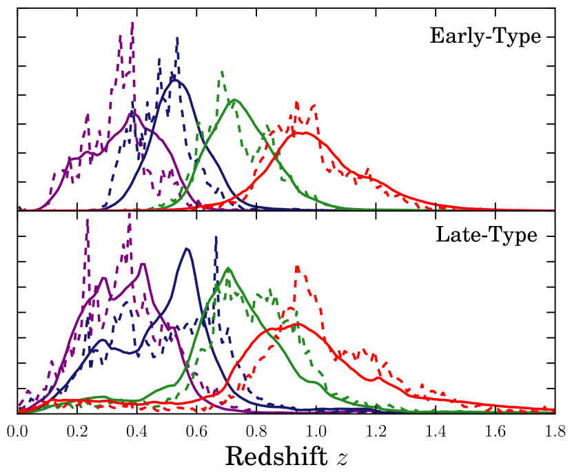
Figure 4: Estimated redshift distributions of the galaxy samples described in this paper. The upper and lower panels show our two Y1 type samples, split according to best-fitting template type $T_{\mathrm{BPZ}}$. The solid curves show estimates derived from the photometric redshift code bpz. The dashed lines are histograms of photo-$z$s for a sample of galaxies from the 32-band COSMOS data, which has been reweighted to match the DES flux and size distribution. Each distribution is independently normalised to unity over the redshift range shown.

In the following we adopt fiducial Gaussian priors for each sample centred according to Table 3 and with widths given by the above calculation.

4 Measurements

In this section we outline the measurements needed to set up the parameter inference detailed in the following section. This section seeks to highlight the new measurements and changes in the Y1 measurement pipeline implemented for this work. Given that the Y1 lens catalogue used here is identical to that in previous work, we simply refer the reader to Elvin-Poole et al. (2017) and Dark Energy Survey Collaboration (2017) for details of the sample selection, binning and two-point measurement.

4.1 Galaxy Shapes

4.1.1 Measurement and Selection Bias

To date, two validated science-ready shear catalogues have been built using the DES Y1 data. The smaller of the catalogues, im3shape, takes a conventional approach to calibrating shear biases, relying on a suite of complex image simulations. A detailed discussion of the processes involved in constructing and testing such a calibration is presented in Zuntz et al. (2017). As we point out in that paper, additional selection can very easily induce multiplicative shear bias.

For this analysis, however, we use the larger of the two shape catalogues. The measurements are made using a technique called metacalibration, the basis of which is to derive the calibration from the data itself using counterfactual copies of each galaxy with additional shear applied. The algorithm remeasures the shear and computes a quantity known as the response:

$$\mbox{\boldmath$R_{\gamma}$}_{i,j}=\frac{e_{i}^{+}-e_{i}^{-}}{\Delta\gamma_{j}},$$ (21)

where $e^{+}$ and $e^{-}$ are the measured values of the ellipticity obtained from images of the same object sheared by $+\gamma$ and $-\gamma$, and $\Delta\gamma=2\gamma$. The galaxy response must be included whenever a shape-derived statistic is calculated. We refer the reader to Sheldon & Huff (2017) and Huff & Mandelbaum (2017) for a full explanation of the algorithm and to Zuntz et al. (2017) for details of the implementation used in DES Y1 and a recipe for applying response corrections.

It is also possible to correct for selection bias using a similar calculation. To do this we must measure the response of the mean ellipticity to the selection function. Imagine for example, we wish to make a cut on galaxy type $T_{\mathrm{BPZ}}$. Since the photometry, and thus $T_{\mathrm{BPZ}}$, are not independent of ellipticity the raw cut may induce shear selection bias. The photometry must be estimated five times per galaxy: once in the original images, and in four counterfactual sheared images. From each set of photometry we re-evaluate $T_{\mathrm{BPZ}}$ and thus derive a slightly different selection mask. A mean response $\langle R_{S}\rangle$ contributed by a selection alone is then defined as the change in ellipticity

$$\mbox{\boldmath$\langle R_{S}\rangle$}_{i,j}\approx\frac{\langle e_{i}\rangle^{S+}-\langle e_{i}\rangle^{S-}}{\Delta\gamma_{j}},$$ (22)

where $\left<e\right>^{S\pm}$ denotes the mean ellipticity measured from the unsheared images, after selection based on quantities measured from the sheared images. The full response for the mean shear is then given by the sum of the shear and selection parts,

$$\mbox{\mbox{\boldmath$\langle R\rangle$}}=\langle\mbox{\mbox{\boldmath$R_{\gamma}$}}\rangle+\langle\mbox{\mbox{\boldmath$R_{S}$}}\rangle.$$ (23)

This must be recalculated each time galaxies are split in any way, including for tomographic binning. For the fiducial early- and late-type samples (divided about $T_{\mathrm{BPZ}}=1$) we obtain a mean selection response of $\left\langle R_{S}\right\rangle_{\mathrm{early}}=0.0018$ and $\left\langle R_{S}\right\rangle_{\mathrm{late}}=-0.0006$ respectively. We obtain a mean response in each sample of $\left\langle R_{\gamma}\right\rangle_{\mathrm{early}}=0.6282$ and $\left\langle R_{\gamma}\right\rangle_{\mathrm{late}}=0.6458$ (compared with $\left\langle R_{\gamma}\right\rangle=0.6416$ for the unsplit Y1 catalogue).

4.1.2 Shear Systematics

In this section we repeat a raft of systematic tests designed to ensure the (sub-)samples used in the following sections are of sufficient quality for cosmology at the precision of DES Y1. Although the full catalogue has been subjected to a rigorous set of tests in Zuntz et al. (2017), it is conceivable that cuts ultimately derived from the observed fluxes could introduce spurious correlations between ellipticity and galaxy properties. The most straightforward diagnostic would simply be to measure the mean shear in bins of observable properties and fit for correlations.

Correlation	Early-Type	Late-Type
PSF $e1$	(-0.0340, 0.0031)	(-0.0270, 0.0017)
PSF $e2$	(0.0014,-0.0338)	(-0.0004,-0.0223)
PSF Size $T_{\mathrm{PSF}}^{1/2}$	(0.0012, 0.0006)	(0.0001, -0.0004)
$S/N$	(0.0001, 0.0008)	(-0.0000(5), 0.0004)
Galaxy Size $T^{1/2}$	(0.0006, 0.0009)	(0.0004, 0.0000(3))

Table 4: Residual correlations between the galaxy ellipticities and observable properties in our fiducial galaxy samples, after weighting by the mean metacalibration derived response. The numbers in each set of parentheses are the correlations between each quantity and the two ellipticity components $(e_{1},e_{2})$. The PSF/galaxy size and signal-to-noise ratio follow the definitions in Zuntz et al. (2017) and Jarvis et al. (2016).

The results of this exercise are shown in Table 4. We test for correlations with a number of observable properties, including seeing (PSF size) and the signal-to-noise of the measurement. As in the unsplit catalogue, the measured correlations are comfortably at the sub-percentage level. We do not consider these to be of concern for cosmological analyses at the precision afforded by our data.

Although we do see a significant non-zero correlation between PSF ellipticity and galaxy shape, the magnitude does not appear to vary significantly as a function of galaxy type. This offers some reassurance that there are not significant selection-based systematics introduced by our cuts. As in Troxel et al. (2017), we measure the mean shear directly in each tomographic bin. In both early- and late-type split samples we report $|e_{1,2}|\lesssim 10^{-4}$ in all redshift bins.

4.2 Two-Point Correlations

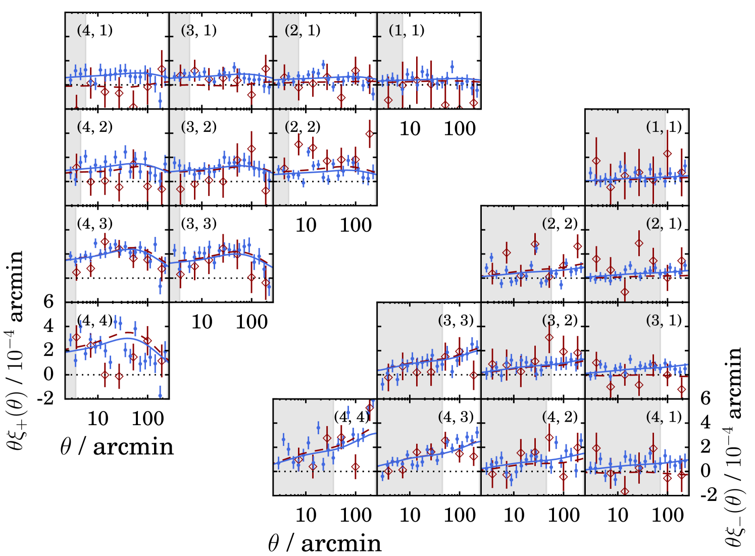
Figure 5: The fiducial cosmic shear datavectors. The filled blue points show the correlation functions measured from the late-type sample described in Section 3.3. Open red diamonds show the same, but for our early-type sample. The solid and dashed lines show the best fitting theoretical prediction for each galaxy sample, as obtained from a $3\times 2$pt analysis. The shaded grey regions indicate the scale cuts for each bin pair, with all points within these areas discarded prior to parameter inference. The reduced $\chi^{2}$ obtained from all points outside the shaded bounds is 1.74 with 59 degrees of freedom for the early-type sample, and 1.28 with 201 degrees of freedom for the late-type sample.

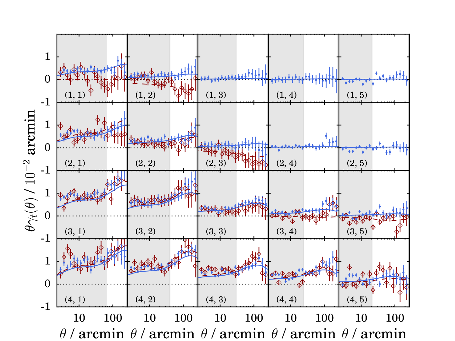
Figure 6: The fiducial galaxy-galaxy lensing datavector. As in Figure 5, filled blue points show measurements on our late-type split sample and open red points show those on early-type galaxies. The numbers in parentheses indicate a pair of redshift bins (source bin, followed by lens). The solid and dashed lines show the best fitting theoretical prediction for late-type and early-type galaxies respectively. The $\chi^{2}$ per degree of freedom obtained from all points outside the shaded bounds (plus the galaxy clustering data $w(\theta)$, which are not shown here) is 1.25 (153 degrees of freedom) for the early-type sample, and 1.22 (204 degrees of freedom) for the late-type sample. A small number of correlations were discarded (and so are missing from this figure) because the estimated redshift distribution of lenses had significant weight above the equivalent distribution of source galaxies.

This work makes use of three sets of correlation function measurements: between galaxy ellipticities, between galaxy positions, and the cross correlation of the two. All two-point measurements presented in this paper make use of TreeCorr . To manage calls to TreeCorr and handle sample selection and binning we make use of a DES-specific python wrapper, which is also publicly available.

The Y1 shear catalogues are used to construct two-point correlation functions of cosmic shear. Our method and choice of statistics and redshift binning follows Troxel et al. (2017). The shear-shear correlations $\xi_{+}$ and $\xi_{-}$ are measured in log-spaced bins in angular scale. To achieve roughly comparable signal-to-noise, measurements on the late-type and blue samples use 20 separation bins, but those on the early-type and red samples use only seven. Galaxy ellipticities are rotated, weighted and averaged in each bin as

$$\xi^{ij}_{\pm}(\theta)=\frac{\sum_{\alpha,\beta}w^{\alpha}w^{\beta}(e_{+}^{\alpha}e_{+}^{\beta}\pm e_{\times}^{\alpha}e_{\times}^{\beta})}{\sum_{\alpha,\beta}w^{\alpha}w^{\beta}(1+m^{\alpha})(1+m^{\beta})}$$ (24)

where the sums run over pairs of galaxies $(\alpha,\beta)$, which are drawn from redshift bins $(i,j)$ and whose angular separation falls within a bin of some finite width $\theta\pm\Delta\theta$. The correlation functions for the fiducial early- and late-type samples used in this paper are shown in Figure 5. Shaded regions corresponding to angular scales discarded in subsequent likelihood calculations.

To avoid the effects of theoretical uncertainties on small scales we impose a lower angular scale cut in each bin. These bounds are relatively stringent compared with contemporary shear analyses and are set out in more detail in Troxel et al. (2017). No angular scales smaller than $\theta_{+}=3.61$ arcmin and $\theta_{-}=36.06$ arcmin are used respectively for $\xi_{+}$ and $\xi_{-}$ correlations. Although designed to remove the potential contamination of baryonic effects, this minimum scale cut also reduces the impact of IA on small scales not captures in the NLA or TATT models. An upper cut of $\theta<250$ arcmin is also imposed to remove scales on which additive shear biases become dominant. The correlation is corrected with an average scale-independent selection response, as outlined by Sheldon & Huff (2017) and Troxel et al. (2017).

Very similar expressions can be constructed for the other two-point correlations used in this work. Following Prat et al. (2017), we use tangential shear about galaxy positions as an estimator for the galaxy-galaxy lensing signal:

$$\gamma_{t}^{ij}(\theta)=\frac{\sum_{\alpha,\beta}w^{\alpha}e_{t}(\alpha|\beta)}{\sum_{\alpha,\beta}(1+m^{\alpha})w^{\alpha}}.$$ (25)

The ellipticity notation $e_{t}(\alpha|\beta)$ represents the $+$ component of source galaxy $\alpha$ relative to the position of lens galaxy $\beta$. Due to the stronger signal-to-noise of the galaxy-galaxy lensing signal, we use 20 bins for both the early- and late-type samples. We make an empirical correction for additive systematics, which commonly affect large scale galaxy-galaxy lensing correlations, by evaluating $\gamma_{t}$ around random points drawn from the Y1 footprint and subtracting the result from the estimated signal around galaxies. The random points are drawn from the DES Y1 footprint, excluding masked regions. For a longer discussion of the random subtraction and the impact it has on the galaxy-galaxy lensing measurement see Prat et al. (2017) (their Sec IV A and Appendix B). We do not incorporate boost factors into this analysis, but rather follow Prat et al. (2017) and apply a scale cut at $12h^{-1}$ Mpc comoving separation (corresponding to the grey shaded portions of Figure 6 ). This is designed to remove scales thought to be significantly impacted by nonlinear bias, and comfortably removes the sections of the data where source-lens contamination is non-negligible. Similarly to with cosmic shear, these minimum scale cuts also reduce potential contamination from IA on fully nonlinear scales.

This analysis explicitly excludes galaxy-galaxy lensing measurements where there is a significant probability that the source galaxy is in front of the lens. That is, we reject correlations where the estimated lens redshift distribution is peaked significantly higher than the source redshift distributions. Due to slight differences in the early- and late-type $n(z)$, this cut removes $\gamma_{t}$ correlations between the lowest early-type redshift bin and the upper three lens bins, but leaves the late-type datavector unchanged.

Finally, the angular clustering auto correlation is constructed, mirroring the choices of Elvin-Poole et al. (2017), from a mixture of galaxy positions $D$ and random points $R$ using the Landy Szalay estimator (Landy & Szalay, 1993),

$$w^{ij}(\theta)=\frac{D^{i}D^{j}-D^{i}R^{j}-R^{i}D^{j}+R^{i}R^{j}}{R^{i}R^{j}}.$$ (26)

The positions in the galaxy catalogue $D$ are sorted into tomographic bins, denoted by the Roman index $i,j$. The random points $R$ are also assigned randomly to tomographic bins, such that the number of randoms per bin matches the number of galaxies. As the sample used for galaxy clustering measurements is the same as that described in Elvin-Poole et al. (2017), we do not show the resulting correlation functions, but refer the reader to Figure 3 of that paper.

The three measurements on the unsplit sample have passed a raft of null tests (Zuntz et al. 2017, Troxel et al. 2017, Prat et al. 2017, Elvin-Poole et al. 2017), and show no indication of significant B-modes. We measure the two-point correlations separately in the full catalogue, and also in our fiducial early-type and late-type samples.

4.3 Covariance Matrix

The covariance matrix of the two-point data is estimated using the CosmoLike software package (Krause & Eifler, 2017). The calculation employs a halo model to generate four-point correlations, which are then used to calculate an analytic non-Gaussian approximation of the multiprobe covariance. For this calculation we assume a flat $\Lambda$CDM universe with cosmological parameters $(\Omega_{\mathrm{m}},\Omega_{\mathrm{b}},\sigma_{8},n_{\mathrm{s}},h)=(0.286,0.05,0.82,0.96,0.7)$. Though the covariance matrix is cosmology dependent, Dark Energy Survey Collaboration (2017) have shown that rerunning the likelihood chains with covariance matrices recomputed at the best fitting cosmology does not induce any significant change in the best fitting parameters obtained from the Y1 data. The CosmoLike covariance code has been tested against log-normal simulations which include the DES survey mask (Krause et al., 2017). Like almost all previous studies of cosmic shear, our covariance matrix does not include the impact of intrinsic alignments. In a similar analysis based on CFHTLenS, Heymans et al. (2013) justify this in two ways. First, the galaxy catalogues used in cosmic shear measurements are typically not dominated by low redshift red population objects, in which IAs are known to be strong (in absolute terms, and relative to the lensing signal). Constraints using mixed samples from contemporary shear surveys have found alignment amplitudes in the range $A_{\mathrm{IA}}\sim 0-1$. The impact on the true covariance of the data due to the presence of IAs is thus expected to be small. Second, the red fraction is typically $\sim 20\%$ or less. Imposing a colour split will leave one with a relatively small red sample, and it is likely its covariance matrix will be dominated by shot noise.

Since the survey properties of DES Y1 are significantly different to those of CFHTLenS, we seek to verify these assumptions. To test this we use a fast analytic code to generate Gaussian covariances for the shear-shear angular power spectrum $C_{\gamma\gamma}$ in DES Y1-like tomographic bins. The IA power spectra are modelled using the NLA model with a range of amplitudes.

We proceed by inspecting the shift in diagonal elements of the covariance matrix. Unsurprisingly (since the dominant GI term will tend to surpress power in the cosmic shear signal) on most scales ignoring IA in the covariance matrix leads one to overestimate the uncertainties. This is particularly true in the autocorrelation of the lower redshift bins. On the largest scales (small $\ell$) this exercise suggests a potential slight underestimation of our errorbars. Mapping this onto a change in parameter space constraints is, however, a non-trivial exercise. We test this explicitly by running a series of MC forecasts on noise-free simulated $C(\ell)$ data using Gaussian covariance matrices with $A_{\mathrm{IA}}=[0,1,3,8]$. The parameter space is identical to that described in Section 2 (all cosmological and nuisance parameters). Using 20 multipole bins in the range $\ell=[5,2000]$ we find no significant change in the marginalised parameter contours between these four cases.

5 Results

This section describes the main results of this paper. We outline the baseline constraints obtained from the colour-split samples described in the earlier sections. The robustness of our results to redshift error and galaxy colour leakage is tested using a series of high-level validation exercises. For comparing IA models run on the same data, we make use of two single-number metrics: the difference in the reduced $\chi^{2}$ at the respective means of the parameter posteriors $\Delta\chi^{2}$ (Krause et al., 2016), and the Bayes Factor $B$ (the ratio of evidence values; see Marshall et al. 2006 for a functional definition and discussion of its usage for cosmological model comparison). The evidence ratios quoted are evaluated using Multinest, but are also tested using the Savage-Dickey approximation, outlined by Trotta (2007). In all cases the two values are seen to agree to $\sim 50\%$ of the Multinest estimate.

5.1 Simultaneous Constaints on Cosmology and Intrinsic Alignments

Our baseline analysis fits three samples independently (early-type, late-type and mixed) using the NLA model for intrinsic alignments in each, and assuming a $\Lambda$CDM cosmology. We will, however, consider a number of more complex IA treatments in the following sections. For reference, the mixed sample $3\times 2$pt cosmology constraints under each of these models are shown in Figure 7 (see also Table 1). In all cases the posterior constraints on $S_{8}$ are statistically consistent, though there are small downwards shifts in some of the models. These individual cases are discussed in more detail below.

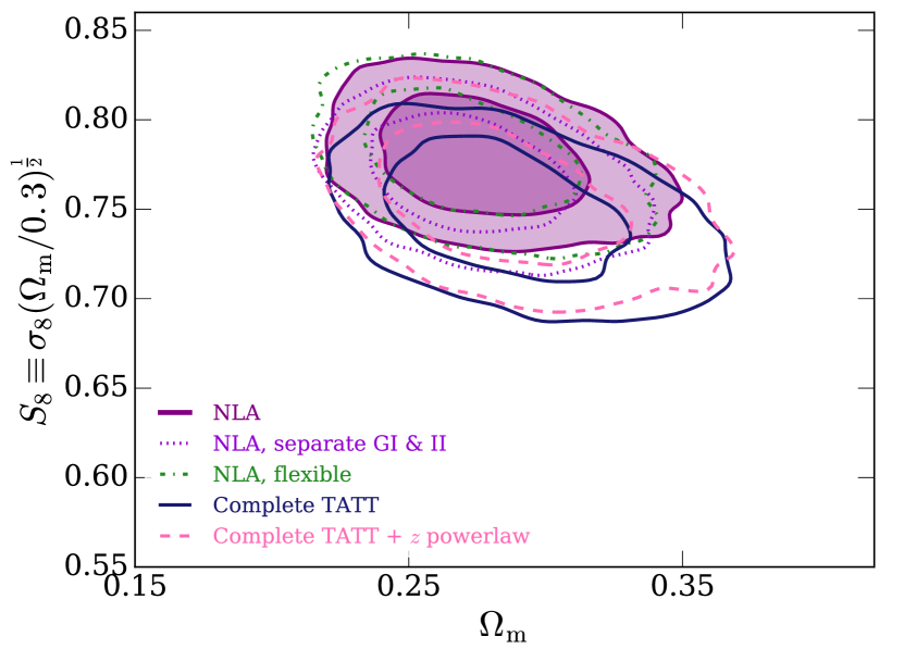
Figure 7: $\Lambda$CDM constraints on $S_{8}$ and $\Omega_{\mathrm{m}}$from cosmic shear, galaxy clustering and galaxy-galaxy lensing, using the unsplit Y1 cosmology sample. The solid filled (purple) contours show the baseline analysis, which assumes the nonlinear alignment model for intrinsic alignments, and is equivalent to the blue contours in Figure 11 of Dark Energy Survey Collaboration (2017). The other lines show extended IA models, the parameters of which are listed in Table 1.

The parameter constraints resulting from the basic analysis are shown in Figure 8. The dashed contours show shear alone, the dotted show the combination of galaxy-galaxy lensing and two-point clustering and the solid (filled) contours show the joint constraints from all three probes. Strikingly, much of the constraining power on the IA model parameters comes from galaxy-galaxy lensing. This can be understood as follows: the II contribution, to which $\gamma_{t}$ is insensitive, is generally subdominant in the NLA model. Combined with the fact that the signal-to-noise on $\gamma_{t}$ is high (compared with the equivalent shear-shear correlations), this allows a relatively strong IA constraint from galaxy-galaxy lensing data. The choice of lens sample is relevant here; the redshift distributions of the redMaGiC lenses overlap strongly with the lower source bins, which boosts the $C_{\delta_{g}\mathrm{I}}$ alignment term. The level of sensitivity of a galaxy-galaxy lensing measurement to IAs will clearly depend on the details of the lens and source redshift distributions. It is, finally, also true that the $\delta_{g}\gamma+\delta_{g}\delta_{g}$ data allows some level of self calibration, effectively breaking the degeneracy between intrinsic alignments and, for example, photometric redshift error.

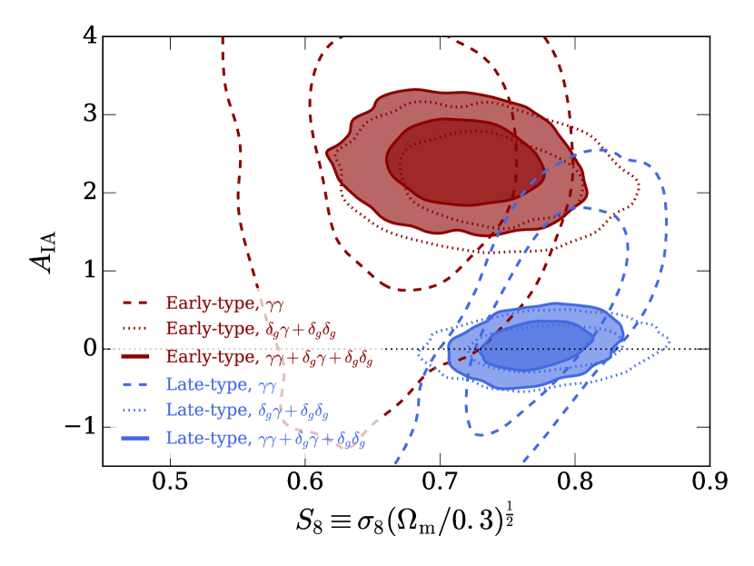
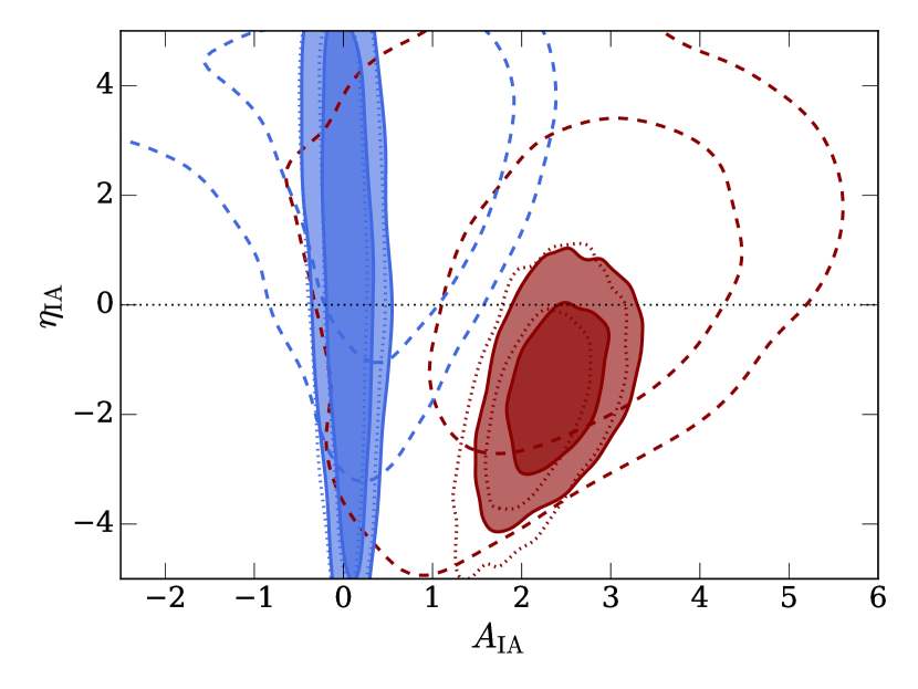
Figure 8: Joint constraints on cosmology and a single NLA model intrinsic alignment amplitude from subpopulations of the DES Y1 fiducial shear catalogue. The two sets of confidence contours are defined by a split according to best-fitting SED, roughly corresponding to early (red) and late (blue) type galaxies.

One notable feature of Figure 8 is the apparent lack of a constraint on the redshift evolution in late-type galaxies. Though it is counterintuitive that the $3\times 2$pt analysis should result in a weaker constraint on $\eta_{\mathrm{IA}}$ than cosmic shear alone, it is understandable in the context of an extended parameter space. The $\delta_{g}\gamma+\delta_{g}\delta_{g}$ data greatly restricts the allowed range of $A_{\mathrm{IA}}$ about zero, which reduces the signal-to-noise of the IA contribution (in the limit $A_{\mathrm{IA}}\rightarrow 0$ one has no ability to constrain $\eta_{\mathrm{IA}}$), resulting in an expansion of the uncertainty on $\eta_{\mathrm{IA}}$.

Under this model all our results are consistent with zero alignments in late-type galaxies at any redshift. In contrast, the IA constraints from the early-type sample are non-zero at the level of $\sim 6.6\sigma$ with the full $3\times 2$pt data. We also find hints of redshift evolution, with negative $\eta_{\mathrm{IA}}$ resulting in a signal that diminishes at high redshifts. It is worth being cautious here, however, given that (a) the deviation from zero is still only just over $1\sigma$, and (b) direct comparison with previous null measurements (e.g. Hirata et al. 2007, Joachimi et al. 2011) are complicated by a basic difference in analysis method. Unlike those studies, we do not explicitly model luminosity dependence in equation 15. The index $\eta_{\mathrm{IA}}$ should thus be interpreted as an effective parameter, which absorbs both genuine evolution of the IA contamination in the same galaxies and the changing composition of the sample along the line of sight.

Considering the final two columns in Table 5, we see a slight improvement in the $\chi^{2}$ of the NLA fit to the early-type sample relative to a case with $A_{\mathrm{IA}}=0$. More noticeably, the Bayes factor appears to strongly disfavour the reduced model in this sample. Though the $\Delta\chi^{2}$ is close to zero, perhaps unsurprisingly, the Bayes factors appear to favour the unmarginalised zero alignment scenario in the late-type sample.

5.2 Robustness to Systematic Errors

In this sub-section we seek to demonstrate that our results do, in fact, provide meaningful information about IAs and are not the result of residual systematic errors in our analysis pipeline.

5.2.1 Shape of the Redshift Distributions

Though it has been shown (Troxel et al., 2017) that DES Y1 shear-only cosmology constraints are insensitive to the precise shape of the redshift distributions, this is not trivially true for IA constraints from sub-divisions of the data. The kernels entering the IA spectra differ significantly from those in cosmic shear alone; it is not inconceivable that the favoured IA parameters derived from these spectra are more sensitive to the details of the $n(z)$ shape than the cosmological parameters. To test this we rerun our six fiducial analysis chains, replacing the smooth PDFs obtained from bpz with histograms of COSMOS redshifts (shown in Figure 4). Since the means of the two sets of distributions per redshift bin are the same by construction, the comparison gives us an estimate for how far reasonable changes to the shape of the $n(z)$ might impact upon our results. The constraints from this test are not shown, but we find only minor changes in the contour size, position and shape for each sample.

5.2.2 Colour Leakage

The previous test offers some reassurance that our photo-$z$ error parameterisation is sufficient. It does not, however, say anything about potential cross contamination between galaxy samples. We next seek to test the impact of potential colour leakage. In Section 4.1.2 we saw leakage affecting the lowest tomographic bin of the early-type sample more strongly than any other selection of the data. To gauge the importance of this we rerun the $\gamma\gamma$ and $\gamma\gamma+\delta_{g}\gamma+\delta_{g}\delta_{g}$ early-type chains, now explicitly excluding any parts of the data vector involving the lowest redshift bin. The result is shown in Figure 9. The best fit of the multivariate posterior is not significantly altered by these cuts, though we see a degradation in statistical power in the shear-only case. In the case of shear alone we also see some level of bimodality about $A_{\rm IA}=0$. We note, however, that similar behaviour has been seen before when adding flexibility to the IA model, particularly in redshift (see, for example, Figure 8 in Dark Energy Survey Collaboration 2016 and to a lesser extent Figure 9 in Joudaki et al. 2017 ). We thus view the opening up of the parameter space as an indication of insufficient information to properly constrain the IA signal without the lowest redshift bin, not as a cause for concern in itself.

A significant caveat here is that the removal of the lowest bin will naturally change the composition of the galaxy sample, which in turn could result in a shift in the IA signal. Unfortunately, it is very difficult to devise a test of leakage that does not. Despite this, the fact that the $3\times 2$pt constraints are almost unchanged by this test is reassuring. It implies that our IA model constraints are not dominated by galaxies in the lowest bin, which in turn implies the leakage seen in that bin is unlikely to be systematically biasing our results from the early-type sample.

Overall, this test does not give us reason to suspect our results are systematically biased by type-leakage.

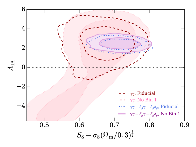
Figure 9: The impact of colour leakage on our fiducial results. The dashed red and dot-dashed blue lines show the baseline $\gamma\gamma$ and $\gamma\gamma+\delta_{g}\gamma+\delta_{g}\delta_{g}$ NLA results for the early-type sample. These are identical to the red dashed and solid lines in Figure 8. The filled pink (dotted) and purple (solid) contours show the equivalent constraints in this parameter space when all two-point correlations involving the lowest lensing redshift bin, which was found to exhibit potentially strong galaxy type cross-contamination, are excluded.

5.2.3 Splitting Method

Since we are using a measured quantity (in our case SED type) as a proxy for galaxy morphology, one would ideally like the result to be independent (within reason) of how that proxy is defined. To test the level at which this is true, we rerun our baseline analysis using the alternative catalogue split described earlier in this paper (‘red’ and ‘blue’ samples; see Section 3.3). The constraints from this alternative split sample are shown in Figure 10. Though the early-type and late-type samples do not map exactly onto the red and blue populations, our results here are very similar to those in the fiducial analysis. The most notable difference is a slight downwards shift in the favoured amplitude $A_{\mathrm{IA}}$ for the red sample compared with early-types. One interpretation for this might be that the early-type sample is a purer population of elliptical pressure-supported galaxies. That is, the red sample suffers from contamination by objects that appear red in colour (e.g. due to dust reddening), but which are morphologically closer to spiral galaxies and more akin to them in their alignment properties. The IA signal is thus diluted and the effective amplitude of the sample is shifted downwards. The qualitative picture is, however, consistent between the two splitting methods.

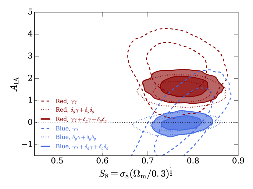
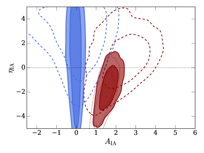
Figure 10: Joint constraints on cosmology and intrinsic alignments using galaxy samples split by photometric colour. The split is implemented independently in each redshift bin using equation 19 and is designed to approximate the evolution of the green valley bimodality in colour-magnitude space.

5.3 Model Extensions

Sample	IA Model	Probe	$A_{1}$	$A_{2}$	Bayes Factor	$\chi^{2}/$ dof
		$\gamma\gamma$	0	0	2.00	$281.4/203=1.39$
Full DES Y1	No IA	$\delta_{g}\gamma+\delta_{g}\delta_{g}$	0	0	$1.74$	$275.1/206=1.34$
		$\gamma\gamma+\delta_{g}\gamma+\delta_{g}\delta_{g}$	0	0	0.83	$582.7/433=1.35$
		$\gamma\gamma$	0	0	1.37	$110.7/61=1.81$
Early	No IA	$\delta_{g}\gamma+\delta_{g}\delta_{g}$	0	0	0.0	$275.1/206=1.34$
		$\gamma\gamma+\delta_{g}\gamma+\delta_{g}\delta_{g}$	0	0	0.0	$570.7/382=1.49$
		$\gamma\gamma$	0	0	11.29	$261.1/203=1.29$
Late	No IA	$\delta_{g}\gamma+\delta_{g}\delta_{g}$	0	0	28.76	$249.7/206=1.21$
		$\gamma\gamma+\delta_{g}\gamma+\delta_{g}\delta_{g}$	0	0	33.25	$530.6/433=1.23$
		$\gamma\gamma$	$1.03^{+0.45}_{-0.57}$	0	1	$276.0/201=1.37$
Full DES Y1	NLA (fiducial)	$\delta_{g}\gamma+\delta_{g}\delta_{g}$	$0.38^{+0.13}_{-0.14}$	0	1	$270.9/204=1.33$
		$\gamma\gamma+\delta_{g}\gamma+\delta_{g}\delta_{g}$	$0.49^{+0.15}_{-0.15}$	0	1	$575.3/431=1.33$
		$\gamma\gamma$	$2.37^{+1.16}_{-0.95}$	0	1	$102.6/59=1.74$
Early	NLA (fiducial)	$\delta_{g}\gamma+\delta_{g}\delta_{g}$	$2.17^{+0.33}_{-0.32}$	0	1	$191.0/153=1.24$
		$\gamma\gamma+\delta_{g}\gamma+\delta_{g}\delta_{g}$	$2.38^{+0.32}_{-0.31}$	0	1	$512.4/380=1.35$
		$\gamma\gamma$	$0.07^{+0.78}_{-1.40}$	0	1	$256.3/201=1.28$
Late	NLA (fiducial)	$\delta_{g}\gamma+\delta_{g}\delta_{g}$	$0.01^{+0.16}_{-0.17}$	0	1	$249.6/204=1.22$
		$\gamma\gamma+\delta_{g}\gamma+\delta_{g}\delta_{g}$	$0.05^{+0.17}_{-0.13}$	0	1	$531.1/431=1.23$
		$\gamma\gamma$	$2.20^{+0.85}_{-1.01}$	0	1.40	$103.5/60=1.72$
Early	TA	$\delta_{g}\gamma+\delta_{g}\delta_{g}$	$2.05^{+0.27}_{-0.25}$	0	$1.35$	$192.9/154=1.35$
		$\gamma\gamma+\delta_{g}\gamma+\delta_{g}\delta_{g}$	$2.17^{+0.27}_{-0.25}$	0	$1.36$	$515.9/381=1.36$
		$\gamma\gamma$	0	$0.08^{+0.47}_{-0.51}$	$9.44$	$260.5/202=1.29$
Late	TT	$\delta_{g}\gamma+\delta_{g}\delta_{g}$	0	$0.04^{+0.41}_{-0.42}$	17.20	$250.2/205=1.22$
		$\gamma\gamma+\delta_{g}\gamma+\delta_{g}\delta_{g}$	0	$-0.11^{+0.45}_{-0.44}$	$15.58$	$532.8/432=1.23$
		$\gamma\gamma$	$0.95^{+0.24}_{-0.29}$,	$-2.25^{+0.65}_{-0.57}$	$0.52$	$266.0/201=1.32$
Full DES Y1	TATT	$\delta_{g}\gamma+\delta_{g}\delta_{g}$	$0.45^{+0.29}_{-0.28}$,	$-0.42^{+1.03}_{-1.05}$	$0.10$	$271.3/204=1.33$
		$\gamma\gamma+\delta_{g}\gamma+\delta_{g}\delta_{g}$	$0.97^{+0.16}_{-0.16}$,	$-2.28^{+0.49}_{-0.47}$	$2.58$	$569.6/431=1.32$
		$\gamma\gamma$	$2.46^{+0.87}_{-1.01}$,	$-3.16^{+2.26}_{-1.44}$	$0.76$	$101.0/59=1.71$
Early	TATT	$\delta_{g}\gamma+\delta_{g}\delta_{g}$	$2.07^{+0.30}_{-0.29}$,	$-0.02^{+0.53}_{-0.51}$	$0.91$	$192.3/153=1.26$
		$\gamma\gamma+\delta_{g}\gamma+\delta_{g}\delta_{g}$	$2.21^{+0.29}_{-0.28}$,	$-0.13^{+0.56}_{-0.48}$	1.20	$515.6/380=1.36$
		$\gamma\gamma$	$0.53^{+0.37}_{-0.51}$,	$-1.08^{+1.45}_{-0.92}$	$0.23$	$255.1/201=1.27$
Late	TATT	$\delta_{g}\gamma+\delta_{g}\delta_{g}$	$-0.00^{+0.20}_{-0.20}$,	$0.03^{+0.51}_{-0.53}$,	0.75	$249.9/204=1.23$
		$\gamma\gamma+\delta_{g}\gamma+\delta_{g}\delta_{g}$	$0.34^{+0.28}_{-0.39}$,	$-1.17^{+1.35}_{-0.90}$	$0.20$	$530.6/431=1.23$
		$\gamma\gamma$	$0.70^{+0.64}_{-1.51}$,	$-1.46^{+1.46}_{-1.25}$	$0.03$	$272.1/199=1.37$
Full DES Y1	TATT ($z$ power law)	$\delta_{g}\gamma+\delta_{g}\delta_{g}$	$0.27^{+0.23}_{-0.20}$,	$0.13^{+0.83}_{-0.81}$	$0.01$	$271.4/202=1.34$
		$\gamma\gamma+\delta_{g}\gamma+\delta_{g}\delta_{g}$	$0.70^{+0.21}_{-0.19}$,	$-1.36^{+0.54}_{-0.70}$	0.07	$568.0/429=1.32$
		$\gamma\gamma$	$1.07^{+1.61}_{-3.77}$,	$-1.68^{+2.06}_{-1.97}$	$0.03$	$104.6/57=1.83$
Early	TATT ($z$ power law)	$\delta_{g}\gamma+\delta_{g}\delta_{g}$	$1.89^{+0.30}_{-0.28}$	$-0.04^{+0.52}_{-0.50}$	$0.32$	$200.3/151=1.27$
		$\gamma\gamma+\delta_{g}\gamma+\delta_{g}\delta_{g}$	$2.17^{+0.40}_{-0.38}$,	$-0.57^{+1.29}_{-1.30}$	0.01	$515.4/378=1.37$
		$\gamma\gamma$	$-1.42^{+1.37}_{-1.51}$,	$-0.51^{+1.48}_{-1.73}$	$35.68$	$253.6/199=1.28$
Late	TATT ($z$ power law)	$\delta_{g}\gamma+\delta_{g}\delta_{g}$	$-0.00^{+0.23}_{-0.21}$,	$-0.09^{+0.87}_{-0.91}$	$0.01$	$250.6/202=1.25$
		$\gamma\gamma+\delta_{g}\gamma+\delta_{g}\delta_{g}$	$0.14^{+0.25}_{-0.27}$,	$-0.66^{+0.94}_{-0.93}$	$0.02$	$532.9/429=1.24$

Table 5: Best-fitting parameters and fit metrics for a selection of the analyses discussed in this paper. The Bayes Factor is defined in this case as the ratio of the evidence obtained from the chain in question relative to that from the NLA model analysis of the same sample.

5.3.1 Separating GI & II

In order to better understand the nature of the IA signal we next introduce a slight generalisation to our fiducial model. Although the linear alignment paradigm has II and GI spectra modulated by the same amplitude, it could argued that one should allow the data to speak for itself where possible. In this spirit, we allow the amplitude and power law index applied to the two IA spectra to vary independently. Our two free alignment parameters are then expanded to four: $\mathbf{p_{\mathrm{IA}}}=(A_{\mathrm{GI}},A_{\mathrm{II}},\eta_{\mathrm{GI}},\eta_{\mathrm{II}})$. The increased flexibility degrades the $S_{8}$ constraint somewhat (see the purple dotted contours in Figure 7), and is accompanied by a small downwards shift in $S_{8}$. From the $3\times 2$pt analyses we obtain marginalised amplitudes of $A^{\mathrm{early}}_{\mathrm{GI}}=2.64^{+0.59}_{-1.20}$, $A^{\mathrm{early}}_{\mathrm{II}}=0.02^{+3.35}_{-3.34}$ and $A^{\mathrm{late}}_{\mathrm{GI}}=0.06^{+0.33}_{-0.34}$, $A^{\mathrm{late}}_{\mathrm{II}}=0.00^{+2.20}_{-2.16}$ for early- and late-type samples respectively. As expected, the GI term correlates with $S_{8}$ (as the GI contribution increases the shear signal becomes increasingly diluted, and so $S_{8}$ must increase to compensate). The II amplitude shows a weaker negative correlation. With no information about the II part coming from the galaxy-galaxy lensing data, the constraint on $A_{\mathrm{II}}$ and $\eta_{\mathrm{II}}$ is relatively weak.

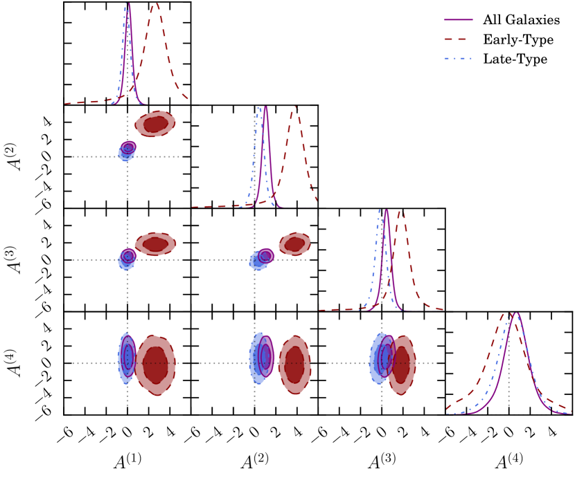
Figure 11: Joint constraints on the amplitudes of the IA spectrum in four tomographic bins for the $\gamma\gamma+\delta_{g}\gamma+\delta_{g}\delta_{g}$ combination. In each case, the red dashed contours show early-type galaxies, the dot-dashed blue show late-types and the shaded contours show the mixed Y1 cosmology sample.

5.3.2 Flexibility in Redshift

We next rerun our fiducial analyses with a free IA amplitude in each redshift bin. This is analogous to our treatment of galaxy bias, and simply modulates the IA power spectra used in the projection integrals. In reality the IA contamination in adjacent redshift slices will, of course, be correlated but we expect the impact to be small and do not attempt to model this here. We show the result of this analysis in Figure 11. Although the late-type signal is consistent with zero at all redshifts, the $A_{\mathrm{IA}}$ amplitude inferred from the early-type sample drops from $\sim 3-4$ in the lower bins to consistent with zero in the upper-most bin. This is consistent with the mildly negative value of $\eta_{\mathrm{IA}}$ seen in the fiducial analysis. As before, it is not possible to separate the effects of the changing composition of the sample from changes in the IA signal for a given set of galaxies. The unsplit sample is relatively stable, with $A^{(i)}\sim 0.5$ in all four redshift bins. As in Troxel et al. (2017), we see a mild degradation of constraints on $S_{8}$ compared with the fiducial model. Where in that paper shifting to the more flexible alignment model was seen to result in a downwards shift in $S_{8}$, however, in the $3\times 2$pt case presented here we find no corresponding shift.

5.3.3 TATT Model (Perturbation Theory)

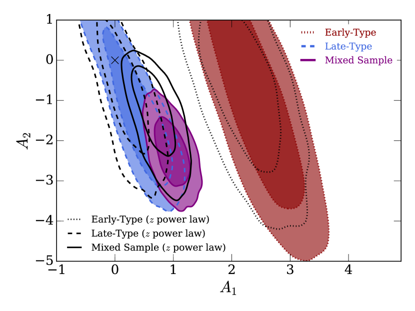
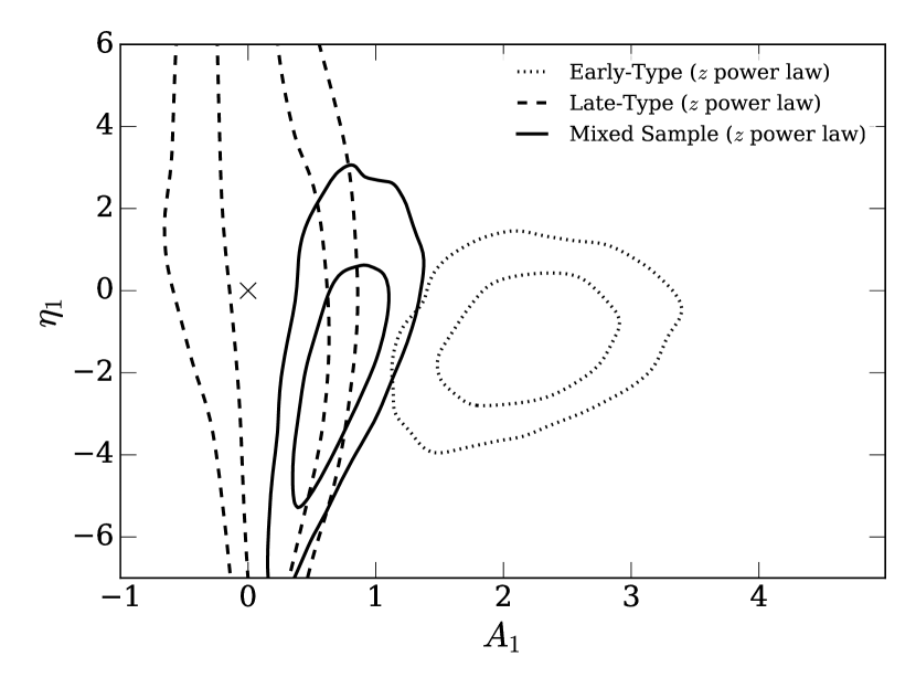
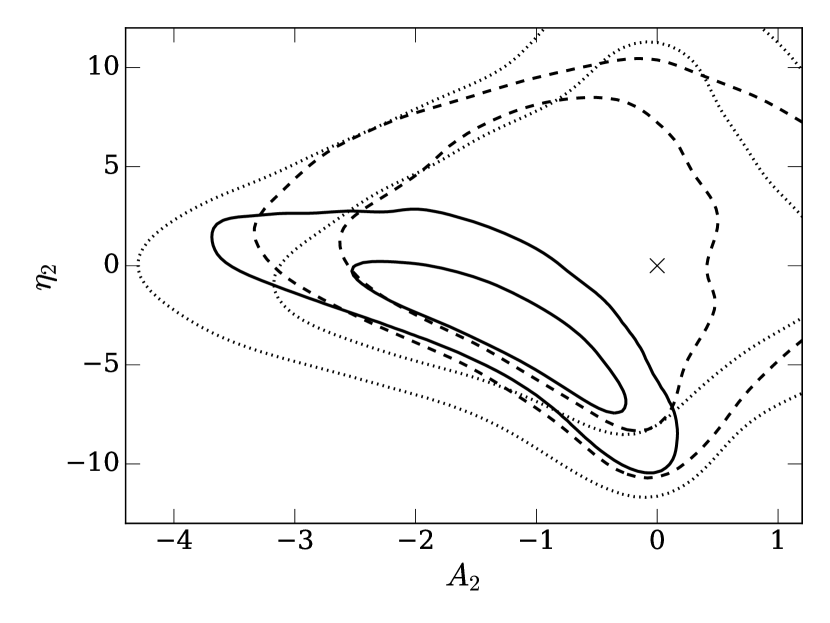
Figure 12: Joint constraints on tidal alignment and tidal torque amplitudes in the TATT model. The three sets of filled contours (dotted red, dashed blue and solid purple) show the results of fitting the baseline TATT model to each of the fiducial early-type, late-type and mixed samples used in this analysis. The unfilled black contours show the same, but with additional power laws in redshift $\eta_{1}$ and $\eta_{2}$, which are also marginalised.

Prior to this point all of the IA models we have considered have been permutations of the Nonlinear Alignment Model. Using this approach for a mixed popluation of galaxies relies on the assumption that the IA contribution to the data is a pure NLA signal, scaled by an effective IA amplitude, which absorbs the dilution due to randomly oriented blue galaxies. In this section we instead employ the TATT model described in Section 2.2.4, which includes linear and quadratic contributions. There are various physically useful variants of this model, with different parameters fixed. For clarity, in the following we will consider, in ascending order of complexity: (a) the TA and TT models, fit to the early-type and late-type samples respectively; (b) the TATT model with no redshift scaling; (c) the TATT model with a free redshift scaling of the form $[(1+z)/(1+z_{0})]^{\eta_{i}}$, $i\in(1,2)$.

In the simplest case (a), the IA model has only one free parameter (either $A_{1}$ or $A_{2}$ for TA and TT respectively), but results in a significantly different IA power spectra (see Figure 2 of Blazek et al. 2017). In the TA fit on the early-type sample, the results closely mirror those from the NLA analysis in Section 5.1; this is unsurprising, given that these models are the same up to the galaxy density weighted term (in the TA model but not NLA), and a redshift scaling (included in the NLA model but not TA). Our results are consistent with the TT IA amplitude in blue galaxies being zero (and also with mildly positive or negative values). The constraints under these models are not shown, but are summarised in Table 5.

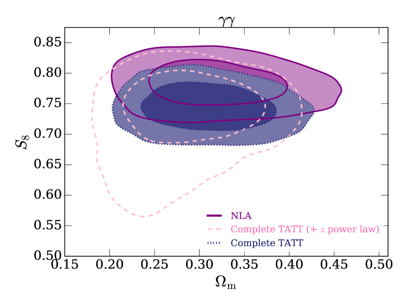
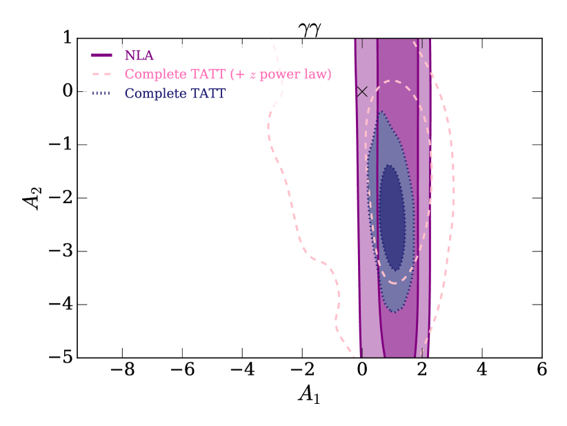
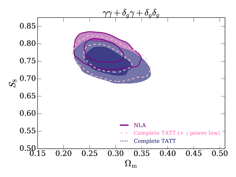
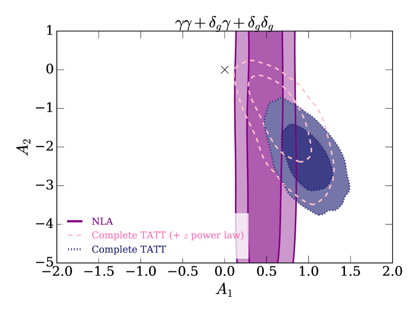
Figure 13: Constraints on cosmological and TATT model parameters in a $\Lambda$CDM cosmology using the full Y1 sample. The upper row shows constraints from cosmic shear alone, and the lower shows the joint constraint using the full $3\times 2$pt datavector. As labelled, we show the baseline NLA constraint (purple filled), the TATT model (blue dotted), and the result using the TATT power spectra, but also marginalising over redshift dependent scaling parameters $\eta_{1}$ and $\eta_{2}$ (pink dashed).

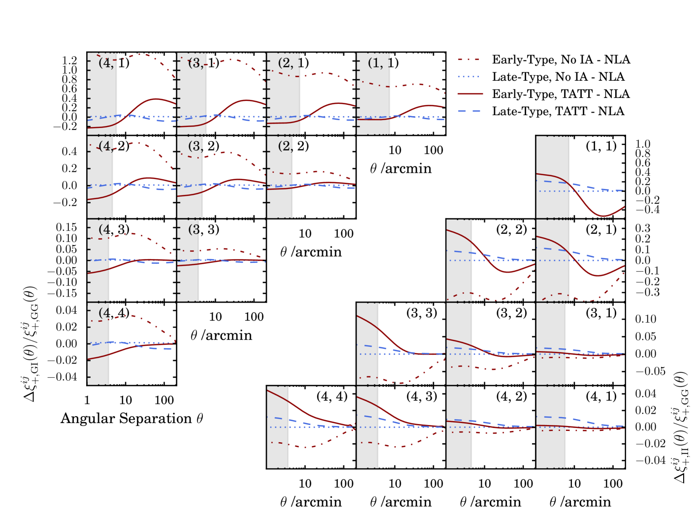
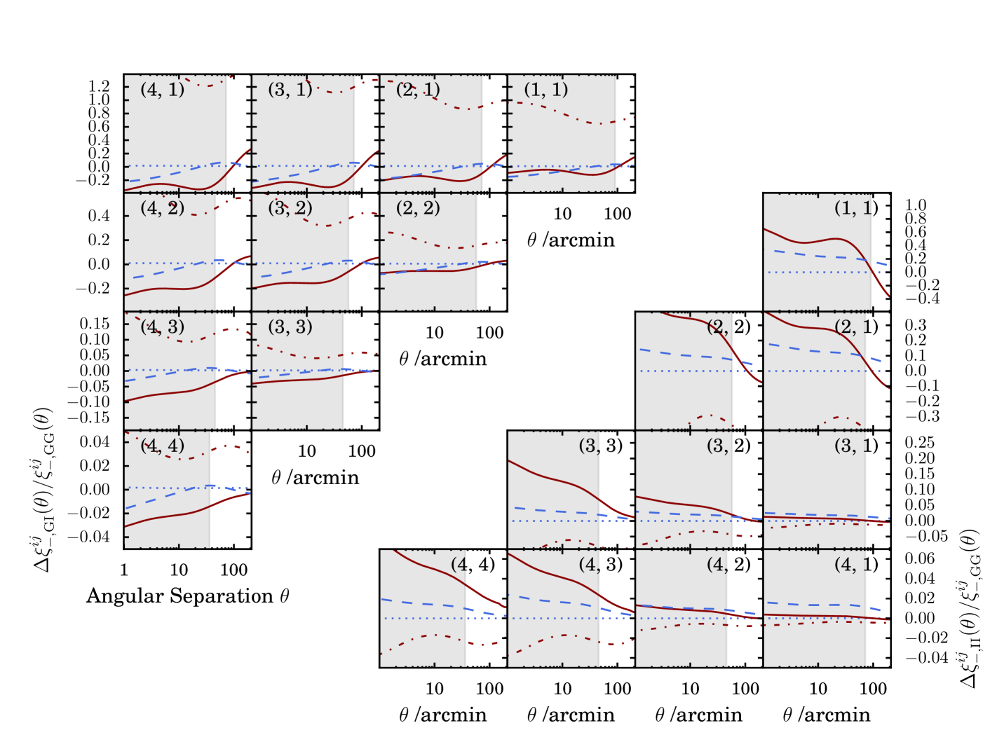
Figure 14: Top: The change in the estimated IA contributions to $\xi_{+}(\theta)$ when switching from the baseline NLA model to different IA scenarios. Red and blue lines show early-type and late-type samples respectively. We generate GI and II power spectra for each model by fixing the relevant parameters to the mean a posteriori values obtained from the 3x2pt analysis using the same model. The shifts between IA contributions $\Delta\xi$ under different models are shown as a fraction of the pure cosmological signal. Dotted and dot-dashed lines show the (No alignments - NLA) shift, while solid and dashed show the (TATT - NLA) difference. The upper and lower triangles show the GI and II contributions respectively. Bottom: The same, but for $\xi_{-}(\theta)$. Each panel shows a particular pair of redshift bins (shown in parentheses). The grey shaded regions indicate angular scales excluded in the likelihood calculations.

The next analysis permutation is to fit for both IA amplitudes, $A_{1}$ and $A_{2}$ simultaneously. Referred to as the TATT model (again, see Table 1 for reference), this model allows for no explicit redshift evolution, with both the indices $\eta_{1}$ and $\eta_{2}$ in equations 17 and 18 fixed to zero. We show the resulting split-sample IA constraints in the upper panel of Figure 12 (filled red/blue contours). The equivalent parameter fits using the unsplit Y1 shape catalogue are shown in Figure 13 (filled dark blue).

There are a number of points worth remarking on here. First, the best fitting $A_{1}$ values are consistent with those from the NLA fits previously, with $A_{1}\sim 2.5$ for early-types and $A_{1}\sim 0$ for late-types. In the split colour samples we report $A_{2}$ is consistent with zero to within $1\sigma$. The mixed Y1 sample, by contrast, favours a negative $A_{2}$ amplitude at the level of a few $\sigma$. Interestingly, the comparison in Figure 13 also suggests that the downwards shift in $S_{8}$ seen when switching to the TATT model is driven by the cosmic shear data (compare the dark blue contours in the upper and lower right-hand panels).

The standard physical interpretation of non-zero $A_{2}$ is as an IA contribution due to tidal torquing. Under the sign convention in equation 18, $A_{2}<0$ implies intrinsic shapes of galaxies are oriented tangentially relative to matter overdensities. This picture is consistent with recent results from hydrodynamic simulations (Chisari et al., 2015), although it is worth bearing in mind that there is still disagreement between simulations with differing methods (e.g. the three dimensional shape-position correlation of disc galaxies in the Illustris and MassiveBlack-II measured by Hilbert et al. 2017 and Tenneti et al. 2016 differ in sign from the equivalent measurement presented in Chisari et al. 2015). There are a number of other facts to note here, however. As ever, mapping IA parameter constraints onto physical processes is non-trivial, as they can very easily absorb features in the data due to residual systematics. We also re-iterate that, even in the absence of systematics, possible non-zero values of both $A_{1}$ and $A_{2}$ in the late-type and mixed samples are not straightforward to interpret. As mentioned above, even in a pure TT scenario, the presence of $A_{2}\neq 0$ can generate an effective non-zero $A_{1}$ amplitude.

We also note that, as in Troxel et al. (2017), the best fitting $S_{8}$ using the TATT model is shifted down slightly relative to the NLA fits; this shift is seen to persist in the full $3\times 2$pt combination. We echo Troxel et al. (2017), however, in warning that this is not necessarily a sign of bias in the NLA results, but could also be a result of an overly flexible model for the constraining power of the data. It is possible to test this idea using simulated data, and to this end we generate a synthetic cosmic shear data vector with zero IAs. We analyse the mock data with the maximally flexible version of TATT (two amplitudes and two power laws). We confirm that, with the Y1 covariance matrix, we do indeed see a downward shift in $S_{8}$ relative to the input. That is, switching to the more complicated model is seen to degrade constraints in the $S_{8}\Omega_{\mathrm{m}}$ plane preferentially towards low $S_{8}$, which results in a $\sim 0.5\sigma$ downward shift in the mean $S_{8}$. This effect is seen to shrink considerably if one assumes a DES Y3 like covariance matrix (both in absolute terms, and in $\sigma$).

Finally in this section, we fit a more flexible version of the TATT model, with a parametrised redshift dependence governed by the additional free parameters $\eta_{1}$ and $\eta_{2}$. As above, we fit each of the early-type, late-type and mixed samples separately. The results can be seen in Figure 12 (black unfilled) and Figure 7 (dashed pink). Note that the cosmic shear TATT + $z$ power law analysis of the mixed sample is almost identical to the “Mixed Model” constraints presented by Troxel et al. (2017). In the mixed galaxy sample we find

$$A^{\mathrm{mixed}}_{1}=0.70^{+0.21}_{-0.19},\quad\quad A^{\mathrm{mixed}}_{2}=-1.36^{+0.54}_{-0.70}.$$ (27)

For early-types we obtain the marginalised mean alignment amplitudes

$$A^{\mathrm{early}}_{1}=2.17^{+0.40}_{-0.38},\quad\quad A^{\mathrm{early}}_{2}=-0.57^{+2.58}_{-2.60},$$ (28)

and for late-type galaxies

$$A^{\mathrm{late}}_{1}=0.14^{+0.25}_{-0.27},\quad\quad A^{\mathrm{late}}_{2}=-0.66^{+1.88}_{-1.86}.$$ (29)

Our results are, again, consistent with the tidal alignment only paradigm for early-type galaxies, and the best-fitting value of the $A_{1}$ amplitude is consistent with the alignment amplitude obtained using the NLA model.

A number of notable differences become apparent when the IA signal is allowed to vary with redshift. First, with $\eta_{2}$ free, the favoured $A_{2}$ in all samples are shifted upwards to slightly less negative values. This is seen most strikingly in the mixed sample (compare the purple and black solid isopleths in Figure 12). The shift results from the crescent-shaped degeneracy seen in the middle panel in Figure 12; fixing $\eta_{2}=0$ forces $A_{2}$ downwards to compensate, but it appears that $A_{2}$ is not sufficiently degenerate with $S_{8}$ for this to translate into a shift in cosmology. Notably there is no region of this parameter space in which either $A_{2}>0$ or $\eta_{2}>0$ is favoured. Under the sign convention used here, $\eta_{2}<0$ implies an IA contribution that declines at high redshift.

In the mixed sample cosmological parameter space (Figure 7, left) the addition of the redshift scaling parameters significantly degrades the quality of the shear-only constraint. In the $3\times 2$pt case (lower left) the extended tail is seen to contract, but notably the posterior peak is not shifted back upwards towards the NLA constraint. It is also worth remarking that the downwards shift when switching to the TATT model, is driven entirely by the shear-shear data. The cosmology constraints from the $2\times 2$pt combination ($\delta_{g}\gamma+\delta_{g}\delta_{g}$; not shown in Figure 13) are close to identical under the NLA, TATT and TATT $+z$ power law models.

Of the TATT model variants discussed above, a small handful provide clearly favourable Bayes factors relative to the NLA analysis. The simplest one-parameter prescriptions yield $B=15.58$ in favour of the TT model in late-types and $B=1.36$ for TA in the early-type sample (interpreted on the Jeffreys’ Scale as “moderate” and “weak” evidence respectively). Under the more complicated models, only the early-type and unsplit TATT fits provide $B>1$. We interpret the low evidence ratios as an indication that the data, including the unsplit Y1 sample, are insufficient to support definitive statements about the relative goodness of fit using the IA models in question.

Finally, to understand at a more basic level how the TATT model enters the two-point observables, we compare simulated datavectors evaluated at the means of the multivariate posterior distributions from our multiprobe TATT and NLA analyses. The solid and dashed lines in Figure 14 show the difference in the IA contribution to the $\gamma\gamma$ data, as predicted by the TATT and NLA models. The upper and lower panels show the change in $\xi_{+}$ and $\xi_{-}$ respectively. The upper and lower triangles within each panel show the GI and II contributions. Since the aim here is to assess the importance of IA modelling uncertainties for cosmology, we show the difference as a fractional shift relative to the cosmological GG signal. For reference we also show (dotted and dot-dashed lines) the difference between the baseline NLA model and a no-alignments scenario. On the scales used in our analysis, the difference tends to be negative, particularly in early-type galaxies. This should be interpreted as saying that the TATT model predicts a smaller IA contribution than the NLA model. In late-type galaxies the reverse is true, suggesting NLA under-predicts the contamination due to IAs. In the correlations involving the upper redshift bins the fractional difference between the models is small ($<10\%$ on all scales), thanks largely to the stronger cosmological signal. In the lowest bins we find the difference can be in excess of $50\%$ of the GG contribution.

5.3.4 $w$CDM Cosmology

The main analyses presented in this work assume a flat $\Lambda$CDM universe. Though there is, to date, no unambiguous observational evidence for deviations from this standard description (see Dark Energy Survey Collaboration 2018a), it is still useful to test how sensitively our conclusions about intrinsic alignments depend upon the cosmological model. A simple, relatively common cosmological extension, is to allow the dark energy equation of state to vary with time; where earlier we enforced $w_{0}=-1$, we now allow it to vary in the range $w_{0}=[-3,-0.333]$. In total we recompute three chains, all using the unsplit Y1 catalogue: one assuming the baseline two-parameter NLA model, and one assuming the TATT IA model with and without redshift power laws. The results are shown in Figure 15. Considering first the IA model constraints, shifting from $\Lambda$CDM to $w$CDM parameter space is seen to induce a slight degradation, but no significant shift in the marginalised distributions (compare the black dashed and purple dotted contours). The mixed data still favour a small positive $A_{1}\sim 1$ and a moderately negative tidal torque amplitude $A_{2}\sim-2.4$. The latter is non-zero at the level of $\sim 2\sigma$. Conversely, if we consider how shifting to a new IA model affects cosmological constraints under $w$CDM, we find the following; as evident from the two left-most columns of Figure 15, switching from NLA to the more sophisticated IA model produces a small shift downwards in both $S_{8}$ and $w_{0}$. It is worth bearing in mind, however, that the parameter constraints under the two models overlap to comfortably within $1\sigma$. The galaxy sample is the same in the two cases, and so both shape noise and cosmic variance are correlated, but it is not straightforwards to assess the significance of such small shifts. As noted before, it is also possible to induce such changes by fitting a model that is too flexible for the data to properly constrain. Computing the Bayes factor of the $w$CDM TATT analysis relative to $w$CDM NLA we find $B=4.22$, which suggests the former IA model is mildly favoured by the Y1 data under the extended cosmology.

This exercise is informative, but not exhaustive. That is, there are a number of other changes to the background cosmology modelling choices (i.e. allowing for non-zero curvature, deviations from general relativity etc) that could plausibly mimic an intrinsic alignment signal. Exploring these degeneracies in detail is, however, an extensive task and considered beyond the scope of the current paper.

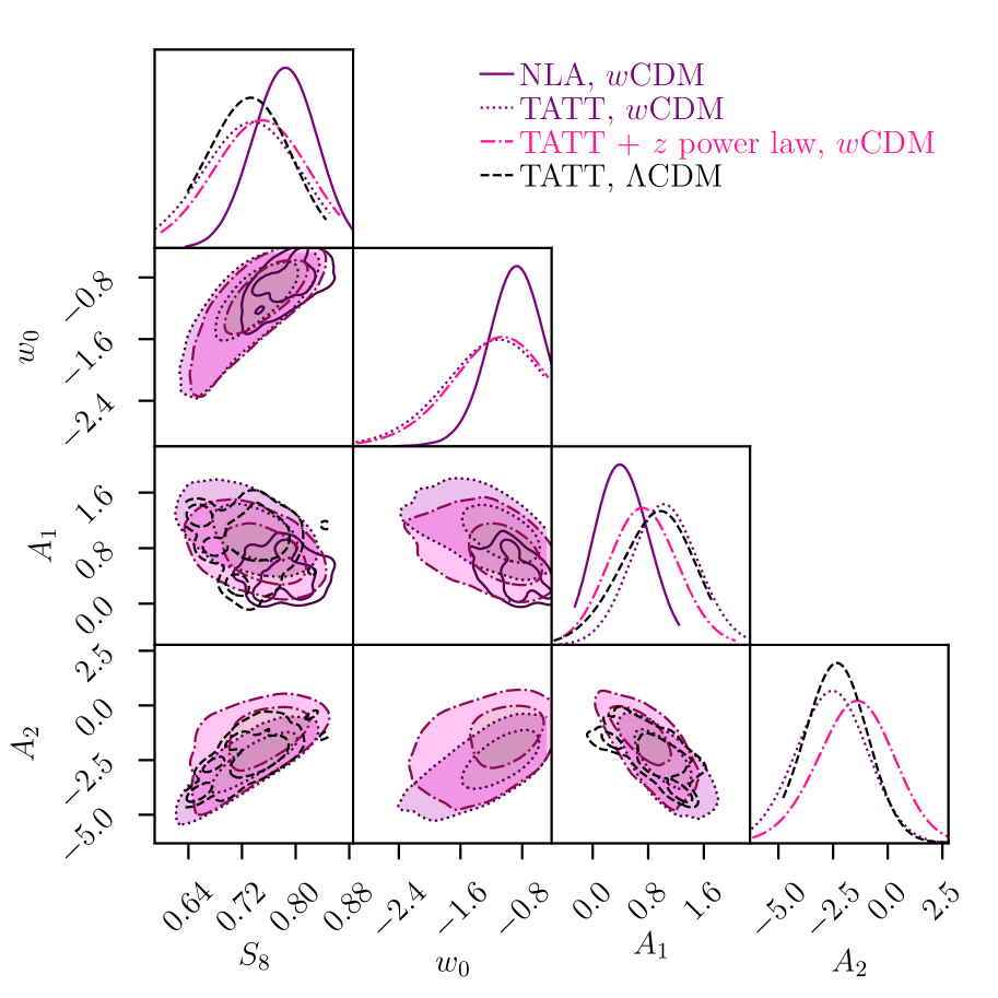
Figure 15: Constraints on IA parameters in the mixed DES Y1 sample. Dark purple (solid) contours show the fiducial NLA model, light purple (dotted) show the TATT model of Blazek et al. (2017) and pink (dash-dotted) show the TATT model with an additional power law in redshift, all assuming a $w$CDM cosmology. The TATT model constraints under $\Lambda$CDM are shown for reference in black (dashed).

5.4 Including Early $\times$ Late Cross Correlations

In this section we incorporate a potential source of information that is systematically excluded from our split-sample analyses: cross correlations between the source galaxy samples. The additional correlations are straightforward to measure, and can be incorporated into our analysis pipeline with minimal code modifications in the same way as extra tomographic bins. The total datavector after including all cross- and auto-correlations between colours and redshift bins consists of 114 unique two-point functions:

• five $w(\theta)$ auto correlations,

• 35 $\gamma_{t}(\theta)$ correlations $(20\times\delta_{g}\gamma^{\mathrm{R}}+15\times\delta_{g}\gamma^{\mathrm{B}}$, excluding galaxy pairs with $\bar{z}_{l}>\bar{z}_{s})$

• 74 $\xi_{+/-}(\theta)$ correlations $(2\times[10\times\gamma^{\mathrm{B}}\gamma^{\mathrm{B}}+10\times\gamma^{\mathrm{R}}\gamma^{\mathrm{R}}+16\times\gamma^{\mathrm{R}}\gamma^{\mathrm{B}}])$

(1171 points with early $\times$ late cross correlations and 811 without, after scale cuts). The superscripts R and B here refer to correlations involving the early- and late-type samples respectively. The additional $\gamma^{\mathrm{R}}\gamma^{\mathrm{B}}$ correlations, along with the extended covariance matrix, which includes all correlations between the two samples, are shown in Appendix D. Modelling the intrinsic alignment contribution to the cross terms is straightforward in both the NLA and TATT models, since the IA in each sample is related to the underlying tidal field. Correlations are then simply given by linear combinations of the tidal field correlations which appear in II contributions to these models, scaled by the relevant $A_{i}$ pre-factors (see Sec. IIIC of Blazek et al. 2017). Under this treatment, the cross terms $(\xi^{\mathrm{RB}}_{\pm})$ are sensitive to both the early- and late-type GI power spectra, and also to a multiplicative combination of the early- and late-type IA amplitudes via the II contribution.

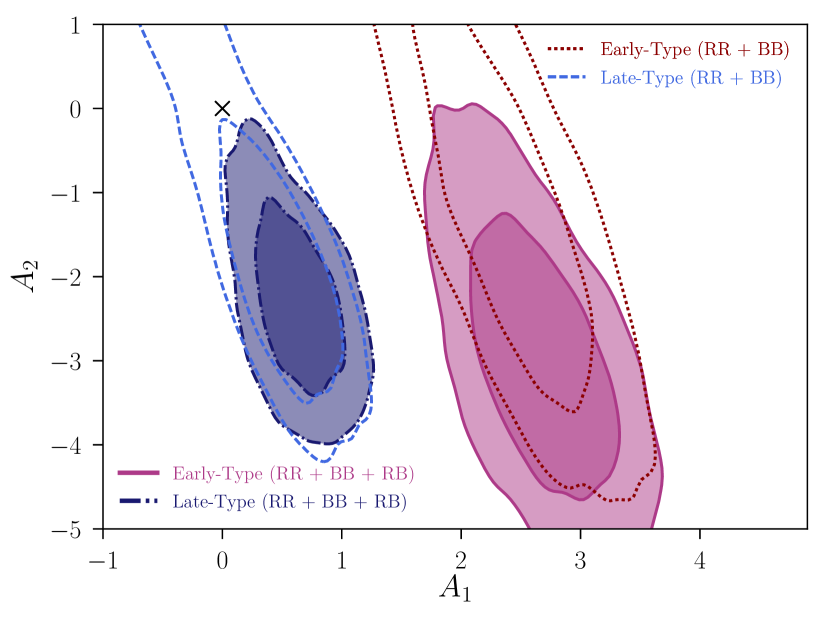
Figure 16: Joint constraints on tidal alignment and tidal torque IA parameters from a simultaneous multicolour $3\times 2$pt analysis of DES Y1. As described in Section 5.4, early- and late-type samples are analysed together using a four-parameter alignment model, with two free amplitudes for each population. The unfilled contours show the constraints from such an analysis using only auto-colour correlations, while the filled contours show the impact of also including early-late cross correlations $\xi^{\mathrm{RB}}_{\pm}$.

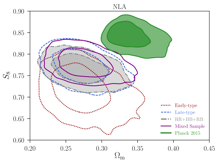
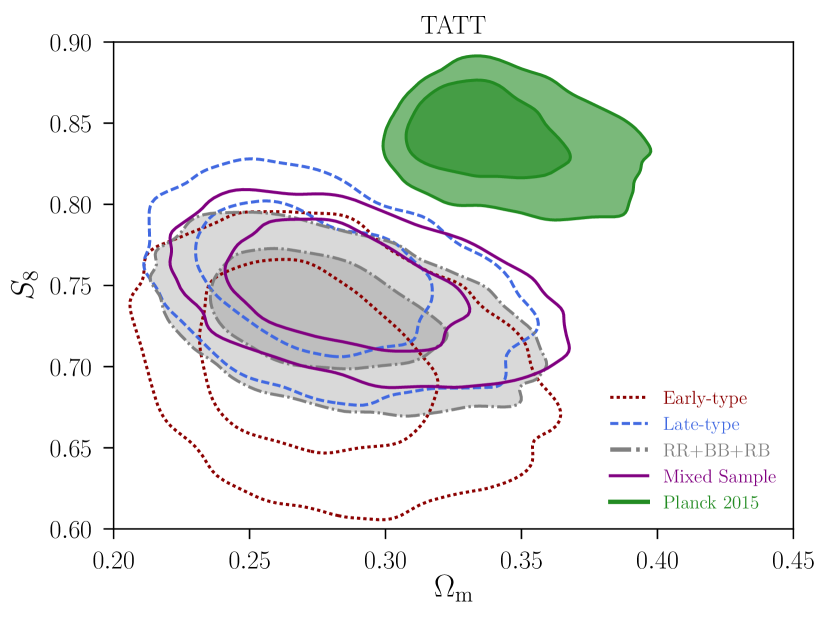
Figure 17: Constraints on cosmological parameters with various intrinsic alignment modelling choices. Left: Using the NLA model with two free parameters $(A_{\mathrm{IA}},\eta_{\mathrm{IA}})$. The open contours show split-sample constraints using early- and late-type source galaxies, while the purple solid show those using the unsplit Y1 source catalogue. Overlain in grey is the posterior distribution obtained from a joint analysis of early-type and late-type galaxies, along with their cross-correlations. This simultaneous fit allows the IA parameters for the early/late samples to vary independently, but does assume the same analytic form for both. Right: As left, but using the Complete TATT model for intrinsic alignments. The filled green contours are identical in the two cases and show the posterior obtained from Planck 2015 temperature and polarization data (TT+EE+TE). Note that, for comparability with our main results, we marginalise over the sum of the neutrino masses here.

In addition to the extra pieces to simulate, it is also necessary to model the covariance of the extended data. As before, we employ CosmoLike to generate a non Gaussian covariance matrix, the details of which can be found in Appendix A of Krause et al. (2016). Note that the non Gaussian contributions are sourced from the single-colour covariance matrices rather than recomputed, an approximation that is tested and seen to have no significant impact on our results in Appendix D.

We repeat our earlier analysis with these multicoloured data, fitting both early-type and late-type IAs simultaneously, along with independent systematics parameters in the two galaxy samples. In the TATT case, this leaves us with four IA parameters $\mathbf{p}_{\mathrm{IA}}=(C_{1}^{\mathrm{R}},C_{1}^{\mathrm{B}},C_{2}^{\mathrm{R}},C_{2}^{\mathrm{B}})$ and a significantly expanded model space (36 free parameters in total, including cosmology and nuisance parameters). We also consider a simultaneous NLA case with parameters $\mathbf{p}_{\mathrm{IA}}=(A_{\mathrm{IA}}^{\mathrm{R}},A_{\mathrm{IA}}^{\mathrm{B}},\eta_{\mathrm{IA}}^{\mathrm{R}},\eta_{\mathrm{IA}}^{\mathrm{B}})$.

The combination of extra data points and greater number of free parameters was found to increase the time required by Multinest to converge significantly. We instead perform this analysis using the Metropolis-Hastings Markov Chain Monte Carlo algorithm of emcee , which uses the affine-invariant sampler of Goodman & Weare (2010). Before accepting a chain as converged we require the following to be true, after burn in: (a) the samples in each parameter cannot be visibly distinguished from random noise of constant mean and variance when plotted in order, (b) no visible difference can be seen between 2D parameter constraints obtained from the first and second halves of the chain and (c) the integrated autocorrelation scale of the chain per walker is much smaller than the total number of samples.

The TATT model constraints resulting from this analysis are shown in Figure 16. In this figure, the unshaded contours show the posteriors from an analysis, which fits cosmology and early/late IAs simultaneously, but excludes the RB cross correlations. The filled contours show the equivalent from the full analysis including all correlations. The agreement of the former with the filled contours in Figure 12) is, of course, expected. The comparison is, however, non-trivial given differences in the sampler, covariance matrix and theory pipeline, in addition to the fact that one is fitting all parameters simultaneously. Although the IA models and nuisance parameters are independent between the two galaxy samples (e.g. BB correlations contain no information about early-type alignments), the simultaneous analysis gives a slightly stronger constraint on cosmology relative to the single-colour analyses, which in turn impacts IA constraints. This is thought to be the source of the small differences in the size of the unfilled contours in Figure 16 relative to those in Figure 12.

The final marginalised IA parameters obtained from the chain including cross correlations are:

$$A^{\mathrm{early}}_{1}=2.66^{+0.67}_{-0.66},\quad\quad A^{\mathrm{early}}_{2}=-2.94^{+1.94}_{-1.83},$$ (30)

and

$$A^{\mathrm{late}}_{1}=0.62^{+0.41}_{-0.41},\quad\quad A^{\mathrm{late}}_{2}=-2.26^{+1.30}_{-1.16},$$ (31)

Although our results hint at a possible non-zero IA signal in a blue galaxy sample, we encourage caution in interpreting this finding. Both IA amplitudes are still consistent with zero at the level of $2\sigma$. It is also worth bearing in mind that, as remarked upon earlier, the combination of a non-zero $A_{2}$ and nonlinear growth can produce an effective $A_{1}$, even if the alignment mechanism is entirely driven by tidal torquing. We note that fixing $A_{2}=0$, as in the various NLA analyses in Section 5.1, returns $A_{1}$ amplitudes consistent with zero in blue galaxies at all redshifts. Though our results taken at face value might suggest both tidal alignment and tidal torquing mechanisms at work in aligning blue galaxies, it is possible that the $A_{1}>0$ value is an artefact of such interplay between the parameters in the TATT model, rather than a genuine indication of physical linear alignment in blue galaxies. It is also worth noting that, as ever with indirect intrinsic alignment measurements, leakage of residual photo-$z$ error into the IA parameters is possible. Though we have attempted to be conservative in our analysis choices, and have tested the response of our baseline results to changes in the details of the $n(z)$, we cannot absolutely rule out photo-$z$ modelling as the source of the apparent non-zero IA signal in late-type galaxies.

Notably, the shear-shear cross correlations appear to contribute a considerable amount of information about IAs in both samples. This is particularly true of $A_{2}$, with the addition of the RB data visibly reducing the size of the shaded contours in Figure 16. That the values are consistent between early- and late-type galaxies is also interesting; though $A_{1}$ differs significantly, there is no clear evidence that the amplitude $A_{2}$ depends on galaxy type.

Finally, we compare the cosmology constraints obtained from the simultaneous analysis described above with our earlier results in Figure 17. In each panel of this figure one IA parameterisation is used for all samples (denoted above each). The unfilled red dotted, blue dashed and purple solid lines show the constraints in this parameter space using the early-type, late-type and unsplit source samples respectively. Overlain in grey we show the constraints from the simultaneous multicolour analysis discussed. One first conclusion to draw here is that splitting the source sample does not bring an obvious degradation in cosmological constraining power. In the late-type only case this is simply a result of the nature of the data excised. The early-type sample accounts for a relatively small fraction of the catalogue (see Table 2). Additionally, it contains a greater abundance of low redshift objects, in which the cosmological shear signal is relatively weak. Perhaps less intuitively, in the fully simultaneous case the additional complexity of the IA model does not appear to be sufficient to significantly broaden the $S_{8}$ posterior.

The downward shift in the TATT model relative to the NLA model is, again, seen here. This has been remarked on previously and we will not discuss it further here. Noticeably, however, we also see a slight downward shift, under both IA models, when one switches from a mixed sample analysis with a single set of effective IA parameters to an explicit colour-split simultaneous one. The magnitude of the shift is approximately the same in both scenarios, and it is worth keeping in mind that the results are still consistent to the level of $\sim 0.5\sigma$.

5.5 Comparison with External Data

As noted in the introduction, cosmic shear and galaxy clustering are far from the only usefully constraining cosmological probe available to the community. CMB measurements offer a particularly powerful way of probing the high-$z$ Universe. To assess the consistency of our measurements with existing results we follow Troxel et al. (2017) and Dark Energy Survey Collaboration (2017) and first recompute the Planck 2015 posterior in our fiducial $\Lambda$CDM parameter space. We use public temperature and polarization measurements (‘Planck TT + lowP’; Planck Collaboration et al. 2016), including scales $\ell=[30–2508]$ and $\ell=[2–29]$ for TT and TT+TE+EE+BB data respectively. The full cosmological parameter space for chains including CMB data has seven free parameters: $A_{\mathrm{s}},n_{\mathrm{s}},\Omega_{\mathrm{m}},\Omega_{\mathrm{b}},h,\Omega_{\nu}h^{2},\tau$. We show the results of this reanalysis in Figure 17 (green contours).

To quantify the consistency of our DES Y1 analysis with the external data we use the ratio:

$$R=\frac{p({\bf D}_{\rm p15},{\bf D}_{\rm DES}|{\rm IA~{}model})}{p({\bf D}_{\rm p15})p({\bf D}_{\rm DES}|{\rm IA~{}model})},$$ (32)

or the ratio of the joint DES + Planck evidence to the product of those obtained from the independent analyses (see Section V of Dark Energy Survey Collaboration 2017 for a fuller explanation). Implicitly, all of the evidence values in Equation 32 assume the same background model for cosmology (i.e. flat $\Lambda$CDM), even if the best fit values for its parameters differ. The evidence ratios derived from the various analysis permutations are listed in Table 6.

It is worth pointing out here that the mixed NLA entry in Table 6 does not match up with the equivalent value reported in Dark Energy Survey Collaboration (2017). This is expected, given that our analysis does not incorporate the updates to the covariance matrix discussed in Troxel et al. (2018).

Here we can see that switching to the TATT model worsens the agreement between DES Y1 and Planck 2015, as quantified by the evidence ratio, by a factor of $\sim 3$. This is consistent with the naive interpretation of the shift in $S_{8}$ between the purple lines in the left- and right-hand panels of Figure 17. Switching to the full multicolour TATT analysis we see a still larger degradation. One should be cautious in drawing strong conclusions from these numbers, however. First of all, we reiterate that we have seen in simulated analyses that slight shifts in $S_{8}$, predominantly downwards, can be achieved by running with an IA model that is not well constrained by the data. Such shifts may be a modelling artefact, and could potentially lead to a false impression of discord. Second, we note that there is some uncertainty on the Multinest evidence values and, potentially, $R$ may have some systematic bias which are neglected in this comparison. With the caveats given above, we note that our reanalysis tends to drive DES away from Planck in cosmological parameter space. Caution should, however, be exercised in drawing conclusions regarding tension from this work; we look to the code fixes and greater statistical power in Y3 to shed light on the matter.

Sample	IA Model	$\mathrm{ln}R$
Mixed	NLA	$-3.65$
Mixed	TATT	$-4.74$
RR+BB+RB	TATT	$-5864.33$

Table 6: Evidence ratios for a subset of the analyses presented in this paper. The evidence ratio $R$ is defined in Equation 32. The term ‘mixed’ here means without colour splitting, and RR+BB+RB refers to the full simultaneous analysis of our early and late-type samples and their cross correlations.

6 Discussion & Conclusions

In this paper we have presented a follow-on study to the Dark Energy Survey Year 1 cosmology results of Troxel et al. (2017) and Dark Energy Survey Collaboration (2017). Using cuts on SED type and photometric colour we have defined early- and late-type galaxy samples. There is prima facie reason to believe that the alignment of intrinsic galaxy shapes should arise by different mechanisms in these galaxy populations, and impact shear two point functions in different ways. From these samples we have obtained large scale cosmic shear, galaxy-galaxy lensing and galaxy clustering measurements, which we have analysed using a selection of different intrinsic alignment models, individually and simultaneously. Our key results are summarised below.

• We have detected a significant difference in IA amplitude between early-type and late-type samples, assuming the NLA model. Early-type galaxies were found to have positive $A_{\mathrm{IA}}\sim 2$ at $\sim 6.5\sigma$. Fits on late-type galaxies were consistent with no intrinsic alignments.

• We have used the split-sample DES data to impose new constraints on IAs and cosmology under the TATT model of Blazek et al. (2017). The linear coefficient $A_{1}$ in early- and late-type galaxies was found to be consistent with the amplitude obtained from fitting the NLA model. We have reported a null measurement of the quadratic term $A_{2}$ in the two subsamples, and a new constraint $A_{2}=-1.36^{+1.08}_{-1.41}$ in the mixed sample.

• We have reported fully simultaneous constraints from the joint analysis of early-type and late-type correlations, plus their cross-correlations. The addition of $\gamma^{\mathrm{R}}\gamma^{\mathrm{B}}$ correlations is seen to tighten constraints on the amplitude of the quadratic term in the TATT model $A_{2}$ particularly. This represents the first hints of non-zero IAs in late-type galaxies from real data, though the physical interpretation is non-trivial.

• We have assessed the differences in cosmology favoured under the various model and data permutations discussed in this work. We have seen the downwards shift in $S_{8}$ seen by Troxel et al. (2017) when switching to the TATT model persists in the $3\times 2$pt case, but is driven by the cosmic shear data. In both NLA and TATT analyses we have seen another downward shift at the level of $\sim 0.5\sigma$ between the unsplit and split simultaneous analyses.

Two ongoing Stage III lensing surveys have now released $3\times 2$pt cosmology analyses, performed by independent groups using separate analysis pipelines, and report consistent results (Dark Energy Survey Collaboration, 2017; van Uitert et al., 2017; Joudaki et al., 2018). Preliminary cosmic shear results from HSC, which will reach deeper than either KiDS or DES, have also very recently been added to the literature (Hikage et al., 2018). Although they represent the state of the art of late-time observational cosmology, the published results from each of these surveys covers less than half of their respective final footprints. Understanding and correctly modelling astrophysical systematics such as intrinsic alignments on both large and small scales will be crucial to the success of these cosmology projects and their successors. The current paper aims to contribute to this effort, providing a detailed study of the large scale intrinsic alignment contamination in DES Y1. Our results come with a number of caveats; notably we choose not to incorporate boost factors into the galaxy-galaxy lensing measurements (justified by scale cuts, which ensure that they have an impact of $\lesssim 1\%$; see Figure 10, Prat et al. 2017). Unfortunately boost factors enter our observables on small scales and where there is a strong overlap between the source and lens redshift distributions, which are precisely the regimes with the most potential for testing IA models. It is thus likely that future analyses on similar lines to this one will need to build these corrections into their pipelines. Our focus here is on large angular scales, which avoids the theoretical complexity of nonlinear growth and the interplay with between IAs and baryonic effects or higher-order galaxy bias. The behaviour of IAs on small scales is an important topic for future investigation, albeit one we consider beyond the scope of this paper.

Nonetheless, our results provide a step towards a more complete understanding of intrinsic alignments in modern lensing surveys. We offer the strongest constraints to date on physically-motivated IA models in a number of validated, realistic lensing samples. Finally, this work lays the ground for future analyses using the considerably larger datasets that will shortly become available. Work is already underway on building lensing measurements from the Dark Energy Survey Year 3 data. Whether or not it proves ultimately necessary to obtain unbiased cosmology constraints, a colour split analysis of the type outlined here will almost certainly be required to test the sufficiency of the IA modelling in future lensing cosmology studies. Our results offer reason for cautious optimism. Though clearly challenging, we have no reason to believe the task of adequately modelling large scale intrinsic alignments to be beyond the theoretical equipment already available to the lensing community.

7 Acknowledgements

The authors would like to thank François Lanusse and Donnacha Kirk for many useful conversations. We are grateful to Catherine Heymans, Elisa Chisari and Rachel Mandelbaum for their thoughts, and to David Bacon, Richard Battye and Sarah Bridle for extensive discussion of an early version of this work. We would also like to thank our anonymous referee for their comments on this work. The numerical analyses presented in this work made use of computing resources at the University of Manchester and Carnegie Mellon University. Correlation function and covariance matrix calculations were performed on the Cori cluster at the National Energy Research and Scientific Computing Center (NERSC; a US DoE facility).

Support for DG was provided by NASA through Einstein Postdoctoral Fellowship grant number PF5-160138 awarded by the Chandra X-ray Center, which is operated by the Smithsonian Astrophysical Observatory for NASA under contract NAS8-03060. JB is supported by an SNSF Ambizione Fellowship.

Funding for the DES Projects has been provided by the U.S. Department of Energy, the U.S. National Science Foundation, the Ministry of Science and Education of Spain, the Science and Technology Facilities Council of the United Kingdom, the Higher Education Funding Council for England, the National Center for Supercomputing Applications at the University of Illinois at Urbana-Champaign, the Kavli Institute of Cosmological Physics at the University of Chicago, the Center for Cosmology and Astro-Particle Physics at the Ohio State University, the Mitchell Institute for Fundamental Physics and Astronomy at Texas A&M University, Financiadora de Estudos e Projetos, Fundação Carlos Chagas Filho de Amparo à Pesquisa do Estado do Rio de Janeiro, Conselho Nacional de Desenvolvimento Científico e Tecnológico and the Ministério da Ciência, Tecnologia e Inovação, the Deutsche Forschungsgemeinschaft and the Collaborating Institutions in the Dark Energy Survey.

The Collaborating Institutions are Argonne National Laboratory, the University of California at Santa Cruz, the University of Cambridge, Centro de Investigaciones Energéticas, Medioambientales y Tecnológicas-Madrid, the University of Chicago, University College London, the DES-Brazil Consortium, the University of Edinburgh, the Eidgenössische Technische Hochschule (ETH) Zürich, Fermi National Accelerator Laboratory, the University of Illinois at Urbana-Champaign, the Institut de Ciències de l’Espai (IEEC/CSIC), the Institut de Física d’Altes Energies, Lawrence Berkeley National Laboratory, the Ludwig-Maximilians Universität München and the associated Excellence Cluster Universe, the University of Michigan, the National Optical Astronomy Observatory, the University of Nottingham, The Ohio State University, the University of Pennsylvania, the University of Portsmouth, SLAC National Accelerator Laboratory, Stanford University, the University of Sussex, Texas A&M University, and the OzDES Membership Consortium.

The DES data management system is supported by the National Science Foundation under Grant Numbers AST-1138766 and AST-1536171. The DES participants from Spanish institutions are partially supported by MINECO under grants AYA2015-71825, ESP2015-88861, FPA2015-68048, SEV-2012-0234, SEV-2016-0597, and MDM-2015-0509, some of which include ERDF funds from the European Union. IFAE is partially funded by the CERCA program of the Generalitat de Catalunya. Research leading to these results has received funding from the European Research Council under the European Union’s Seventh Framework Program (FP7/2007-2013) including ERC grant agreements 240672, 291329, and 306478. We acknowledge support from the Australian Research Council Centre of Excellence for All-sky Astrophysics (CAASTRO), through project number CE110001020.

This manuscript has been authored by Fermi Research Alliance, LLC under Contract No. DE-AC02-07CH11359 with the U.S. Department of Energy, Office of Science, Office of High Energy Physics. The United States Government retains and the publisher, by accepting the article for publication, acknowledges that the United States Government retains a non-exclusive, paid-up, irrevocable, world-wide license to publish or reproduce the published form of this manuscript, or allow others to do so, for United States Government purposes.

Based in part on observations at Cerro Tololo Inter-American Observatory, National Optical Astronomy Observatory, which is operated by the Association of Universities for Research in Astronomy (AURA) under a cooperative agreement with the National Science Foundation.

Appendix A Degeneracies between IA Parameters and Source Galaxy Bias

In this appendix we explore the level at which uncertainty in the galaxy bias in our lensing sample affects our resuts. Though source galaxy bias does not enter standard NLA prescription, the Complete TATT model includes additional terms generated by the fact that measurements occur, by definition, where there are observable galaxies, which leads to a density weighting that is sensitive to the galaxy bias in the source population Blazek et al. (2015).

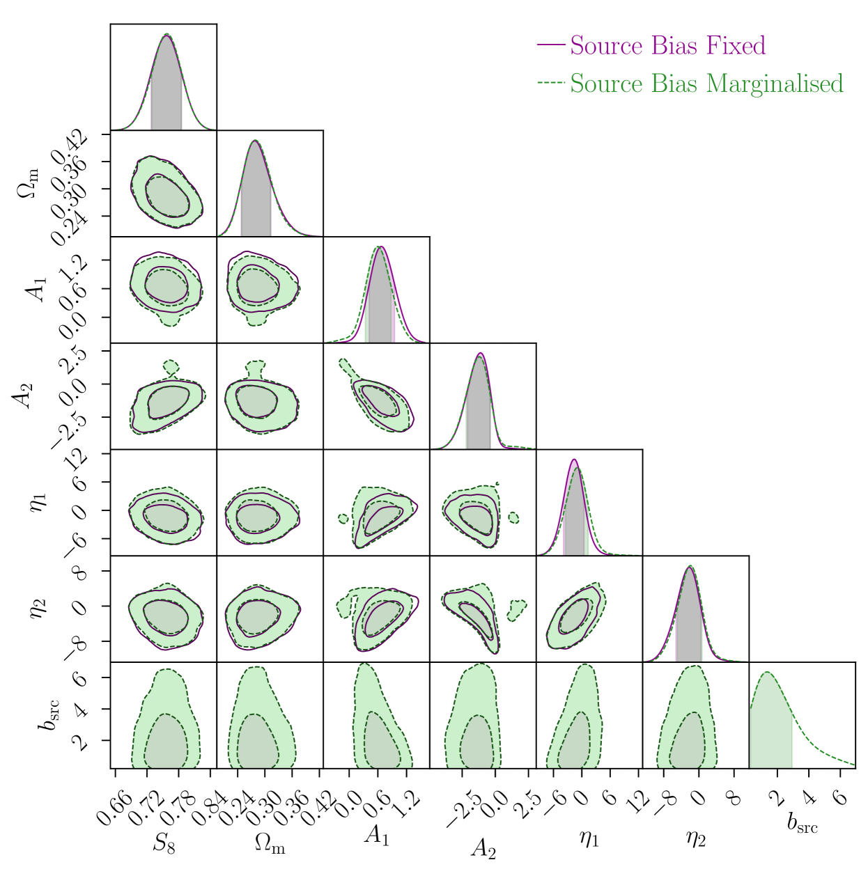
Figure 18: Constraints on cosmology, intrinsic alignment parameters and source galaxy bias in the mixed Y1 sample, assuming a mixed tidal alignment plus tidal torque model, and using all three correlations ($\gamma\gamma+\delta_{g}\gamma+\delta_{g}\delta_{g}$). Solid lines show the result with source galaxy bias fixed at $b_{g}^{\mathrm{src}}=1$ and the dashed green lines show the case where $b_{g}^{\mathrm{src}}$ is allowed to vary.

In the main body of this paper, we assume the angular scale cuts imposed are sufficiently stringent to ensure linear galaxy bias. Unlike lens bias, which appears directly in our predictions of $\gamma_{t}(\theta)$ and $w(\theta)$ and is always marginalised, our main analysis fixes the source bias $b_{g}^{\mathrm{src}}$ to unity, independent of scale, redshift and galaxy sample. Although from a theoretical perspective we do not expect this to have a major impact on our results, we test this assumption in practice here. To this end we made a small modification to the TATT prediction code, which allows $b_{g}^{\mathrm{src}}$ to be varied as a single redshift independent nuisance parameter. We then rerun the mixed TATT analysis with a flat prior on $b_{g}^{\mathrm{src}}=[0.1,8]$. The results are shown in Figure 18.

One should note that we show only the TATT results here; mathematically $b_{g}^{\mathrm{src}}$ appears in the TA terms and the TA/TT interaction terms (see Section III C of Blazek et al. 2017), and does not enter the picture in a pure tidal torquing scenario. It is apparent that the cosmological results are largely unaffected. We do see a slight upwards shift in the redshift index $\eta_{1}$, in the mixed sample. This is, however, most likely an artefact of our chosen parameter volume rather than a sign that our main result for this sample is biased. Although our assumption that $b_{g}^{\mathrm{src}}>0.1$ is justified by simulations and previous lensing measurements, $b_{g}^{\mathrm{src}}$ is only weakly constrained by the $3\times 2$pt data, and we are in effect artificially truncating the parameter space. Without this cut off, the joint posterior of $\eta_{1}$ and $b_{g}^{\mathrm{src}}$ would extend further into the $\eta_{1}<0$ regime, which would shift the constraints slightly closer to the fiducial results in which $b_{g}^{\mathrm{src}}$ is fixed. We also test the sensitivity of the early-type and late-type only results (both TATT and individual TA and TT) to marginalising over source bias. We see no significant change in the findings presented in the main sections of this paper. These analyses also provide some information (albeit weak at best) on the galaxy bias in the two source samples. In early type galaxies we find $b_{g}^{\mathrm{src}}\sim 0.1-2.5$. The bias in late-types is very poorly constrained, providing no preferred value in the range $b_{g}^{\mathrm{src}}=[0.1-7.0]$, thanks largely to the low amplitude of the IA signal in these galaxies, and the fact that the dominant alignment, if present, is expected to come through the tidal torquing, which is insensitive to source galaxy bias at next-to-leading order.

Appendix B The Impact of Neutrinos on Galaxy Bias

In the main sections of this study two other notable changes were introduced relative to Dark Energy Survey Collaboration (2017). First, the impact of neutrinos on halo bias (and ultimately galaxy bias) were omitted, whereas Krause & Eifler (2017) and Dark Energy Survey Collaboration (2017) include an analytic scale-dependent modification using the prescription of LoVerde (2014). Note that the first order effect of neutrino free-streaming on the shape of the matter power spectrum, is included in our modelling. As in the main DES Y1 analyses we marginalise over the total neutrino mass $\Omega_{\nu}h^{2}$ using wide flat priors. The impact of neutrinos through a slight modification to the galaxy bias (referred to for the sake of brevity as “neutrino bias”) is small, and one would not expect their inclusion to have a significant bearing on results at the scale cuts and statistical power of DES Y1. Krause & Eifler (2017) demonstrate this to be the case for the main Y1 results under the NLA model. We explicitly test their findings hold true for our split samples, under the TATT model.

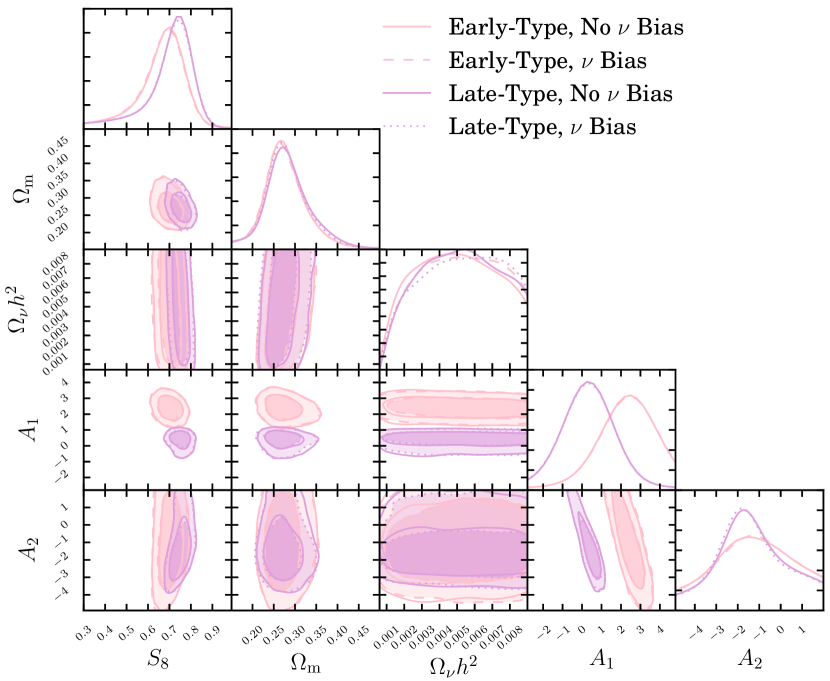
Figure 19: $3\times 2$pt constraints on cosmology and intrinsic alignment parameters from DES Y1 early- and late-type samples, assuming the Complete TATT IA model described in Section 2.2.4. The unfilled solid lines show the results for the two samples presented in the main body of this paper and the filled contours show the equivalent, but with an additional step in the theory calculation to model the impact of massive neutrinos on galaxy bias. In all cases the source galaxy bias is fixed at $b_{g}^{\mathrm{src}}=1$ and a flat $\Lambda$CDM cosmology is assumed.

We do not seek to propagate the impact of neutrinos to the source galaxy bias, but given the results of Appendix A this is not expected to alter our findings. Rerunning the multiprobe TATT analysis (with two free IA parameters $A_{1}$ and $A_{2}$ only), we obtain the results shown in Figure 19. No significant change in the constraints on any particular parameter are observed.

Appendix C Intrinsic Alignment Induced B-modes

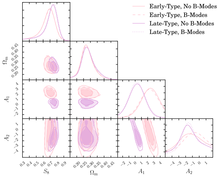
Figure 20: $3\times 2$pt constraints on cosmology and intrinsic alignment parameters from DES Y1 early- and late-type samples, assuming the Complete TATT IA model described in Section 2.2.4. The unfilled solid lines show the results for the two samples presented in the main body of this paper and the filled contours show the equivalent with additional B-modes contributions to the IA power spectra. In all cases the source galaxy bias is fixed at $b_{g}^{\mathrm{src}}=1$ and a flat $\Lambda$CDM cosmology is assumed.

The TATT model predicts a B-mode contribution to the II power spectrum, which was omitted in the results shown in the main body of this work. To test the robustness of our results to this, we rerun the early-type and late-type TATT analyses. The pipeline now includes an additional stage, in which at each step in parameter space we compute $P_{\mathrm{II}}^{BB}(k)$ using Blazek et al. (2017)’s equation 39, transform it to angular space via the Limber integral for a particular pair of redshift bins $ij$ and add the result to $C^{ij}_{\mathrm{II}}(\ell)$. The split analyses with and without B-modes are shown in Figure 20. Note that the filled contours represent the two galaxy samples; the offset between them should not be interpreted as the bias due to the IA B-mode contribution. The impact on all parameter constraints barring $A_{2}$ are close to negligible. Though the impact on $A_{2}$ is non-trivial, the shift is comfortably with the level of precision allowed by DES Y1.

Appendix D Multicolour Cross Correlations: Measurements & Covariance Matrix

The analysis of Section 5.4 includes a slight expansion of the total datavector. That is, the multicolour datavector is larger than the union of the early- and late-type datavectors due to cross-colour shear-shear correlations. The measurements are performed using the same code pipeline with minimal modifications to allow multiple colour bins to be handled simultaneously. The resulting cross-correlations are shown in Figure 21 ($\xi_{+}$ in purple, $\xi_{-}$ in pink).

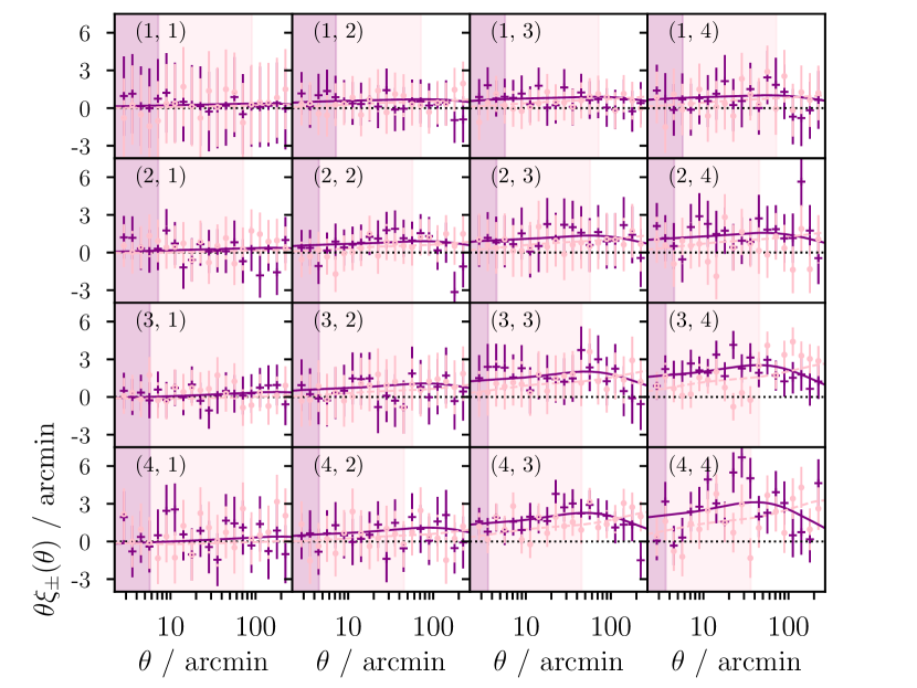
Figure 21: Multicolour cross correlations, as measured from the Y1 early- and late-type samples described in this work. Each panel shows the correlation between bin pair $(i,j)$, where $i\in(1,2,3,4)$ is the redshift bin index for the early-type galaxies used in the correlation, and $j$ is that for late-types. In each case purple crosses show $\xi_{+}$ and pink dots show $\xi_{-}$. The shaded regions in the same colours indicate the scale cuts applied to each of these measurements.

In order to obtain covariance matrices for the extended multicolour $3\times 2$pt data, we use the halo model implemented in CosmoLike (see Appendix A, Krause et al. 2016. In this scheme each element of the covariance matrix is evaluated as the sum of three contributions,

$$\mathrm{Cov}\left[C^{ij}_{\alpha\beta}(\ell)C^{kl}_{\delta\gamma}(\ell^{\prime})\right]=\\ \mathrm{Cov}^{\mathrm{G},ijkl}_{\alpha\beta\delta\gamma}(\ell,\ell^{\prime})+\mathrm{Cov}^{\mathrm{NG},ijkl}_{\alpha\beta\delta\gamma}(\ell,\ell^{\prime})+\mathrm{Cov}^{\mathrm{SSC},ijkl}_{\alpha\beta\delta\gamma}(\ell,\ell^{\prime}),$$ (33)

where the upper Roman indices indicate redshift and colour bins and the lower Greek ones denote a particular observable probe. The Gaussian piece is given by the standard expression

$$\mathrm{Cov}^{\mathrm{G},ijkl}_{\alpha\beta\delta\gamma}(\ell,\ell^{\prime})=\frac{4\pi\delta_{\ell\ell^{\prime}}}{A(2\ell+1)\Delta\ell}\times\\ \left[\tilde{C}^{ik}_{\alpha\delta}(\ell)\tilde{C}^{jl}_{\beta\gamma}(\ell)+\tilde{C}^{il}_{\alpha\gamma}(\ell)\tilde{C}^{jk}_{\beta\delta}(\ell)\right].$$ (34)

This is sensitive to the total survey area $A$ and the spacing of discrete $\ell$ modes $\Delta\ell$. The tilde indicates the sum of a cosmic variance term and a noise term, $\tilde{C}_{\mu\nu}^{ab}=C_{\mu\nu}^{ab}+N^{ab}_{\mu\nu}$. The shot/shape noise is nonzero only for $\mu=\nu$ and $i=j$, and is given by $N^{ij}_{\gamma\gamma}=\sigma_{e}^{2}/2n^{i}_{g}$ in the case of cosmic shear and $N^{ij}_{\delta_{g}\delta_{g}}=1/n_{g}^{i}$ for galaxy clustering. The first non Gaussian contribution is given by Krause et al. 2016’s equation A3 and is obtained by integrating the product of the trispectrum $T^{ijkl}_{\alpha\beta\gamma\delta}$ (sensitive to galaxy bias and cosmology) and four lensing efficiencies (sensitive to the normalised redshift distributions) over $\ell$ and $\chi$. This term is, then, dependent on the shape of the reshift distributions, but not on the absolute number densities. Similarly, the super-sample covariance contribution is sensitive to the redshift distributions, cosmology and the survey geometry, but is independent of the source number density.

Given the relatively high computational cost of generating the full multicolour non Gaussian covarance matrix we instead draw the non Gaussian and super sample covariance contributions from the single colour matrices, as follows. CosmoLike is first run to generate a base $2240\times 2240$ Gaussian covariance matrix. The non Gaussian contribution to an element $a,b$ is selected from:

• The early-type covariance matrix if $a,b$ is in blocks $\mathrm{Cov}[\xi^{\mathrm{RR}}_{+},\xi^{\mathrm{RR}}_{+}]$, $\mathrm{Cov}[\xi^{\mathrm{RR}}_{-},\xi^{\mathrm{RR}}_{-}]$, $\mathrm{Cov}[\xi^{\mathrm{RR}}_{+},\xi^{\mathrm{RR}}_{-}]$, $\mathrm{Cov}[\xi^{\mathrm{RR}}_{+},\gamma^{\mathrm{R}}_{t}]$, $\mathrm{Cov}[\xi^{\mathrm{RR}}_{+},w]$ or $\mathrm{Cov}[\gamma^{\mathrm{R}}_{t},w]$ of the covariance matrix

• The late-type covariance matrix if $a,b$ is in any other block.

We emphasise here that this patching process is used only to obtain the (relatively small) non Gaussian contribution to the multicolour covariance matrix; the Gaussian part, which contains shot/shape noise terms is clearly sensitive to the galaxy number densities, as so must be recomputed in full for the extended data vector.

The validity of our approach thus relies on the qualitative similarity of the redshift distributions of the two samples, such that the non Gaussian contributions for bin pair $ij$ are insensitive to whether the samples being correlated are RR, BB or RB. The resulting multiprobe matrices include non Gaussian (up to trispectrum) contributions and supersample variance. We show the resulting correlation matrix in Figure 22. We test the impact of the approximation described above by rerunning our TATT parameter constraints using the late-type part of the multicolour data vector only (i.e. applying cuts to remove all correlations involving early-type galaxies). The results are compared with those from the single colour late-type data vector, for which we generated the non Gaussian covariance matrix in full, in Figure 23. The purple solid and dark blue dashed contours show the constraints using the two non Gaussian covariance matrices. For reference, the green dotted contour shows the impact of ignoring the non Gaussian contribution entirely. We have chosen to show only the late-type sample here, given that its higher number density means that it is less shape noise dominated, and so more sensitive to changes in the non Gaussian covariance contribution.

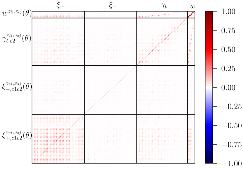
Figure 22: Correlation matrix for the multiprobe multicolour datavector. The matrix contains $2240\times 2240$ elements, and includes shear $(\xi_{\pm})$, galaxy-galaxy lensing $(\gamma_{t})$ and galaxy clustering $(w)$ measurements, including all cross correlations between the various statistics. Within each block, elements are grouped by $\theta$ bin, then by redshift bin couplet and finally by galaxy type pairing.

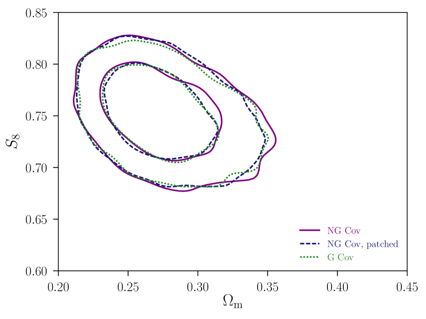
Figure 23: Cosmology constraints from the late-type galaxy sample, assuming different approximations for the covariance matrix. The solid purple line shows the $3\times 2$pt constraints using a non Gaussian covariance matrix, obtained from CosmoLike and used in Sections 5.1. The dashed dark blue contours are obtained using the multicolour covariance matrix described in the text and used in Section 5.4 (a baseline Gaussian matrix plus non Gaussian contributions sourced from the single colour matrices). Dotted green show the equivalent from the same data using a Gaussian covariance matrix (not used for any of the results presented in the main body of this paper, but included here for reference).

Including these extra data and using the covariance matrix described above, we obtain a reduced $\chi^{2}$ at the best-fitting cosmology of 1.11. This compares with $849.1/774=1.10$ for the simultaneous early-late analysis without cross-correlations (and with 1.36 and 1.23 respectively for the early- and late-type only TATT analyses).

The signal-to-noise of the combined $3\times 2$pt multicolour data (defined in terms of the datavector and covariance matrix $\mathcal{S}=\left(\sum_{i}\sum_{j}D_{i}C_{ij}^{-1}D_{j}^{T}\right)^{0.5}$ (see equation 15 in Chang et al. 2018) is 85.5. Deconstructed into single two point statistic values, we obtain 30.7, 21.4 and 30.5 for $\xi_{+}$, $\xi_{-}$ and $\gamma_{t}$ respectively. For early-type galaxies the corresponding values are 15.9, 9.9 and 19.7 and for late-types we find 20.2, 15.4 and 26.3.

Author Affiliations

¹McWilliams Center for Cosmology, Department of Physics, Carnegie Mellon University, Pittsburgh, PA 15213, USA
²Center for Cosmology and Astro-Particle Physics, The Ohio State University, Columbus, OH 43210, USA
³Laboratory of Astrophysics, é Ecole Polytechnique Fédérale de Lausanne (EPFL), Observatoire de Sauverny, 1290 Versoix, Switzerland
⁴Department of Physics, The Ohio State University, Columbus, OH 43210, USA
⁵Department of Astronomy/Steward Observatory, 933 North Cherry Avenue, Tucson, AZ 85721-0065, USA
⁶Institut de Física d’Altes Energies (IFAE), The Barcelona Institute of Science and Technology, Campus UAB, 08193 Bellaterra (Barcelona) Spain
⁷Kavli Institute for Particle Astrophysics & Cosmology, P. O. Box 2450, Stanford University, Stanford, CA 94305, USA
⁸SLAC National Accelerator Laboratory, Menlo Park, CA 94025, USA
⁹Jet Propulsion Laboratory, California Institute of Technology, 4800 Oak Grove Dr., Pasadena, CA 91109, USA
¹⁰ Department of Physics & Astronomy, University College London, Gower Street, London, WC1E 6BT, UK
¹¹ Department of Physics, ETH Zurich, Wolfgang-Pauli-Strasse 16, CH-8093 Zurich, Switzerland
¹² Max Planck Institute for Extraterrestrial Physics, Giessenbachstrasse, 85748 Garching, Germany
¹³ Universitäts-Sternwarte, Fakultät für Physik, Ludwig-Maximilians Universität München, Scheinerstr. 1, 81679 München, Germany
¹⁴Argonne National Laboratory, 9700 South Cass Avenue, Lemont, IL 60439, USA
¹⁵Scottish Universities Physics Alliance, Institute for Astronomy, University of Edinburgh, Edinburgh EH9 3HJ, UK
¹⁶ Cerro Tololo Inter-American Observatory, National Optical Astronomy Observatory, Casilla 603, La Serena, Chile
¹⁷ Fermi National Accelerator Laboratory, P. O. Box 500, Batavia, IL 60510, USA
¹⁸ Department of Physics and Astronomy, University of Pennsylvania, Philadelphia, PA 19104, USA
¹⁹ CNRS, UMR 7095, Institut d’Astrophysique de Paris, F-75014, Paris, France
²⁰ Sorbonne Universités, UPMC Univ Paris 06, UMR 7095, Institut d’Astrophysique de Paris, F-75014, Paris, France
²¹ Jodrell Bank Centre for Astrophysics, School of Physics and Astronomy, University of Manchester, Oxford Road, Manchester, M13 9PL, UK
²² Centro de Investigaciones Energéticas, Medioambientales y Tecnológicas (CIEMAT), Madrid, Spain
²³ Laboratório Interinstitucional de e-Astronomia - LIneA, Rua Gal. José Cristino 77, Rio de Janeiro, RJ - 20921-400, Brazil
²⁴ Department of Astronomy, University of Illinois at Urbana-Champaign, 1002 W. Green Street, Urbana, IL 61801, USA
²⁵ National Center for Supercomputing Applications, 1205 West Clark St., Urbana, IL 61801, USA
²⁶ Institut d’Estudis Espacials de Catalunya (IEEC), 08034 Barcelona, Spain
²⁷ Institute of Space Sciences (ICE, CSIC), Campus UAB, Carrer de Can Magrans, s/n, 08193 Barcelona, Spain
²⁸ Observatório Nacional, Rua Gal. José Cristino 77, Rio de Janeiro, RJ - 20921-400, Brazil
²⁹ George P. and Cynthia Woods Mitchell Institute for Fundamental Physics and Astronomy, and Department of Physics and Astronomy, Texas A&M University, College Station, TX 77843, USA
³⁰ Department of Physics, IIT Hyderabad, Kandi, Telangana 502285, India
³¹ Excellence Cluster Universe, Boltzmannstr. 2, 85748 Garching, Germany
³² Faculty of Physics, Ludwig-Maximilians-Universität, Scheinerstr. 1, 81679 Munich, Germany
³³ Kavli Institute for Cosmological Physics, University of Chicago, Chicago, IL 60637, USA
³⁴ Instituto de Fisica Teorica UAM/CSIC, Universidad Autonoma de Madrid, 28049 Madrid, Spain
³⁵ Department of Astronomy, University of Michigan, Ann Arbor, MI 48109, USA
³⁶ Department of Physics, University of Michigan, Ann Arbor, MI 48109, USA
³⁷ Santa Cruz Institute for Particle Physics, Santa Cruz, CA 95064, USA
³⁸ Harvard-Smithsonian Center for Astrophysics, Cambridge, MA 02138, USA
³⁹ Australian Astronomical Optics, Macquarie University, North Ryde, NSW 2113, Australia
⁴⁰ Departamento de Física Matemática, Instituto de Física, Universidade de São Paulo, CP 66318, São Paulo, SP, 05314-970, Brazil
⁴¹ Department of Astronomy, The Ohio State University, Columbus, OH 43210, USA
⁴² Department of Astrophysical Sciences, Princeton University, Peyton Hall, Princeton, NJ 08544, USA
⁴³ Institució Catalana de Recerca i Estudis Avançats, E-08010 Barcelona, Spain
⁴⁴ Brookhaven National Laboratory, Bldg 510, Upton, NY 11973, USA
⁴⁵ School of Physics and Astronomy, University of Southampton, Southampton, SO17 1BJ, UK
⁴⁶ Instituto de Física Gleb Wataghin, Universidade Estadual de Campinas, 13083-859, Campinas, SP, Brazil
⁴⁷ Computer Science and Mathematics Division, Oak Ridge National Laboratory, Oak Ridge, TN 37831
⁴⁸ Institute of Cosmology and Gravitation, University of Portsmouth, Portsmouth, PO1 3FX, UK
⁴⁹ Argonne National Laboratory, 9700 South Cass Avenue, Lemont, IL 60439, USA
$\dagger$ Einstein Fellow

References

- Abbott et al. (2018) Abbott T. M. C., et al., 2018, preprint, (arXiv:1810.02322)
- Baldauf et al. (2010) Baldauf T., Smith R. E., Seljak U., Mandelbaum R., 2010, Phys. Rev. D, 81, 063531
- Baxter et al. (2018) Baxter E. J., et al., 2018, preprint, (arXiv:1802.05257)
- Benítez (2000) Benítez N., 2000, ApJ, 536, 571
- Blazek et al. (2011) Blazek J., McQuinn M., Seljak U., 2011, J. Cosmology Astropart. Phys., 5, 010
- Blazek et al. (2012) Blazek J., Mandelbaum R., Seljak U., Nakajima R., 2012, J. Cosmology Astropart. Phys., 5, 041
- Blazek et al. (2015) Blazek J., Vlah Z., Seljak U., 2015, J. Cosmology Astropart. Phys., 8, 015
- Blazek et al. (2017) Blazek J., MacCrann N., Troxel M. A., Fang X., 2017, arXiv:1708.09247,
- Bridle & King (2007) Bridle S., King L., 2007, New Journal of Physics, 9, 444
- Brown et al. (2002) Brown M. L., Taylor A. N., Hambly N. C., Dye S., 2002, MNRAS, 333, 501
- Carlstrom et al. (2011) Carlstrom J. E., et al., 2011, PASP, 123, 568
- Catelan et al. (2001) Catelan P., Kamionkowski M., Blandford R. D., 2001, MNRAS, 320, L7
- Chang et al. (2018) Chang C., et al., 2018, preprint, (arXiv:1808.07335)
- Chisari & Dvorkin (2013) Chisari N. E., Dvorkin C., 2013, J. Cosmology Astropart. Phys., 12, 029
- Chisari et al. (2014) Chisari N. E., Mandelbaum R., Strauss M. A., Huff E. M., Bahcall N. A., 2014, MNRAS, 445, 726
- Chisari et al. (2015) Chisari N., et al., 2015, MNRAS, 454, 2736
- Chisari et al. (2016) Chisari N. E., Dvorkin C., Schmidt F., Spergel D. N., 2016, Phys. Rev. D, 94, 123507
- Croft & Metzler (2000) Croft R. A. C., Metzler C. A., 2000, ApJ, 545, 561
- Dark Energy Survey Collaboration (2016) Dark Energy Survey Collaboration 2016, Phys. Rev. D, 94, 022001
- Dark Energy Survey Collaboration (2017) Dark Energy Survey Collaboration 2017, Submitted to Phys. Rev. D, arXiv:1708.01530,
- Dark Energy Survey Collaboration (2018a) Dark Energy Survey Collaboration 2018a, To be Submitted to Phys. Rev. D,
- Dark Energy Survey Collaboration (2018b) Dark Energy Survey Collaboration 2018b, MNRAS, 480, 3879
- Davis et al. (2017) Davis C., et al., 2017, preprint, (arXiv:1710.02517)
- Desjacques et al. (2018) Desjacques V., Jeong D., Schmidt F., 2018, Phys. Rep., 733, 1
- Drlica-Wagner et al. (2018) Drlica-Wagner A., et al., 2018, ApJS, 235, 33
- Elvin-Poole et al. (2017) Elvin-Poole J., et al., 2017, Submitted to Phys. Rev. D, arXiv:1708.01536,
- Faltenbacher et al. (2009) Faltenbacher A., Li C., White S. D. M., Jing Y.-P., Shu-DeMao Wang J., 2009, Research in Astronomy and Astrophysics, 9, 41
- Fang et al. (2017) Fang X., Blazek J. A., McEwen J. E., Hirata C. M., 2017, J. Cosmology Astropart. Phys., 2, 030
- Feroz et al. (2013) Feroz F., Hobson M. P., Cameron E., Pettitt A. N., 2013, preprint, (arXiv:1306.2144)
- Flaugher et al. (2015) Flaugher B., et al., 2015, AJ, 150, 150
- Gatti et al. (2018) Gatti M., et al., 2018, MNRAS, 477, 1664
- Goodman & Weare (2010) Goodman J., Weare J., 2010, Communications in Applied Mathematics and Computational Science, Vol.~5, No.~1, p.~65-80, 2010, 5, 65
- Harnois-Déraps et al. (2017) Harnois-Déraps J., et al., 2017, MNRAS, 471, 1619
- Heavens (2003) Heavens A., 2003, MNRAS, 343, 1327
- Heymans & Heavens (2003) Heymans C., Heavens A., 2003, ArXiv Astrophysics e-prints,
- Heymans et al. (2005) Heymans C., et al., 2005, MNRAS, 361, 160
- Heymans et al. (2013) Heymans C., et al., 2013, MNRAS, 432, 2433
- Hikage et al. (2018) Hikage C., et al., 2018, preprint, (arXiv:1809.09148)
- Hilbert et al. (2017) Hilbert S., Xu D., Schneider P., Springel V., Vogelsberger M., Hernquist L., 2017, MNRAS, 468, 790
- Hildebrandt et al. (2017) Hildebrandt H., et al., 2017, MNRAS, 465, 1454
- Hirata & Seljak (2004) Hirata C. M., Seljak U., 2004, Phys. Rev. D, 70, 063526
- Hirata et al. (2007) Hirata C. M., Mandelbaum R., Ishak M., Seljak U., Nichol R., Pimbblet K. A., Ross N. P., Wake D., 2007, MNRAS, 381, 1197
- Hoyle et al. (2017) Hoyle B., et al., 2017, Submitted to MNRAS, arXiv:1708.01532,
- Huff & Mandelbaum (2017) Huff E., Mandelbaum R., 2017, arXiv:1702.02600,
- Jarvis et al. (2016) Jarvis M., et al., 2016, MNRAS, 460, 2245
- Jee et al. (2016) Jee M. J., Tyson J. A., Hilbert S., Schneider M. D., Schmidt S., Wittman D., 2016, ApJ, 824, 77
- Joachimi & Bridle (2010) Joachimi B., Bridle S. L., 2010, A&A, 523, A1
- Joachimi & Schneider (2010) Joachimi B., Schneider P., 2010, preprint, (arXiv:1009.2024)
- Joachimi et al. (2011) Joachimi B., Mandelbaum R., Abdalla F. B., Bridle S. L., 2011, A&A, 527, A26
- Joachimi et al. (2013) Joachimi B., Semboloni E., Hilbert S., Bett P. E., Hartlap J., Hoekstra H., Schneider P., 2013, MNRAS, 436, 819
- Joachimi et al. (2015) Joachimi B., et al., 2015, Space Sci. Rev., 193, 1
- Joudaki et al. (2017) Joudaki S., et al., 2017, MNRAS, 465, 2033
- Joudaki et al. (2018) Joudaki S., et al., 2018, MNRAS, 474, 4894
- Kiessling et al. (2015) Kiessling A., et al., 2015, Space Sci. Rev., 193, 67
- King & Schneider (2003) King L. J., Schneider P., 2003, A&A, 398, 23
- Kirk et al. (2012) Kirk D., Rassat A., Host O., Bridle S., 2012, MNRAS, 424, 1647
- Kirk et al. (2015) Kirk D., et al., 2015, Space Sci. Rev., 193, 139
- Köhlinger et al. (2017) Köhlinger F., et al., 2017, MNRAS, 471, 4412
- Krause & Eifler (2017) Krause E., Eifler T., 2017, MNRAS, 470, 2100
- Krause et al. (2016) Krause E., Eifler T., Blazek J., 2016, MNRAS, 456, 207
- Krause et al. (2017) Krause E., et al., 2017, Submitted to Phys. Rev. D, arXiv:1706.09359,
- Kwan et al. (2017) Kwan J., et al., 2017, MNRAS, 464, 4045
- Laigle et al. (2016) Laigle C., et al., 2016, ApJS, 224, 24
- Landy & Szalay (1993) Landy S. D., Szalay A. S., 1993, ApJ, 412, 64
- Larsen & Challinor (2016) Larsen P., Challinor A., 2016, MNRAS, 461, 4343
- Leistedt et al. (2016) Leistedt B., et al., 2016, ApJS, 226, 24
- Leonard & Mandelbaum (2018) Leonard C. D., Mandelbaum R., 2018, preprint, (arXiv:1802.08263)
- Li et al. (2013) Li C., Jing Y. P., Faltenbacher A., Wang J., 2013, ApJ, 770, L12
- LoVerde (2014) LoVerde M., 2014, Phys. Rev. D, 90, 083530
- MacCrann et al. (2018) MacCrann N., et al., 2018, MNRAS, 480, 4614
- Mackey et al. (2002) Mackey J., White M., Kamionkowski M., 2002, MNRAS, 332, 788
- Mandelbaum (2015) Mandelbaum R., 2015, Journal of Instrumentation, 10, C05017
- Mandelbaum (2017) Mandelbaum R., 2017, preprint, (arXiv:1710.03235)
- Mandelbaum et al. (2006) Mandelbaum R., Hirata C. M., Ishak M., Seljak U., Brinkmann J., 2006, MNRAS, 367, 611
- Mandelbaum et al. (2011) Mandelbaum R., et al., 2011, MNRAS, 410, 844
- Mandelbaum et al. (2013) Mandelbaum R., Slosar A., Baldauf T., Seljak U., Hirata C. M., Nakajima R., Reyes R., Smith R. E., 2013, MNRAS, 432, 1544
- Marshall et al. (2006) Marshall P., Rajguru N., Slosar A., 2006, Phys. Rev. D, 73, 067302
- McEwen et al. (2016) McEwen J. E., Fang X., Hirata C. M., Blazek J. A., 2016, J. Cosmology Astropart. Phys., 9, 015
- Mishra-Sharma et al. (2018) Mishra-Sharma S., Alonso D., Dunkley J., 2018, preprint, (arXiv:1803.07561)
- Okumura & Jing (2009) Okumura T., Jing Y. P., 2009, ApJ, 694, L83
- Parkinson et al. (2012) Parkinson D., et al., 2012, Phys. Rev. D, 86, 103518
- Planck Collaboration et al. (2016) Planck Collaboration et al., 2016, A&A, 594, A1
- Planck Collaboration et al. (2018) Planck Collaboration et al., 2018, arXiv e-prints, p. arXiv:1807.06205
- Prat et al. (2017) Prat J., et al., 2017, Submitted to Phys. Rev. D, arXiv:1708.01537,
- Ross et al. (2011) Ross A. J., et al., 2011, MNRAS, 417, 1350
- Rozo et al. (2016) Rozo E., et al., 2016, MNRAS, 461, 1431
- Schaan et al. (2017) Schaan E., Krause E., Eifler T., Doré O., Miyatake H., Rhodes J., Spergel D. N., 2017, Phys. Rev. D, 95, 123512
- Schmitz et al. (2018) Schmitz D. M., Hirata C. M., Blazek J., Krause E., 2018, J. Cosmology Astropart. Phys., 7, 030
- Schneider & Bridle (2010) Schneider M. D., Bridle S., 2010, MNRAS, 402, 2127
- Sheldon & Huff (2017) Sheldon E. S., Huff E. M., 2017, arXiv:1702.02601,
- Simon et al. (2013) Simon P., et al., 2013, MNRAS, 430, 2476
- Singh & Mandelbaum (2016) Singh S., Mandelbaum R., 2016, MNRAS, 457, 2301
- Singh et al. (2015) Singh S., Mandelbaum R., More S., 2015, MNRAS, 450, 2195
- Takahashi et al. (2012) Takahashi R., Sato M., Nishimichi T., Taruya A., Oguri M., 2012, ApJ, 761, 152
- Tenneti et al. (2016) Tenneti A., Mandelbaum R., Di Matteo T., 2016, MNRAS, 462, 2668
- Tonegawa et al. (2017) Tonegawa M., Okumura T., Totani T., Dalton G., Yabe K., 2017, preprint, (arXiv:1708.02224)
- Trotta (2007) Trotta R., 2007, MNRAS, 378, 72
- Troxel & Ishak (2015) Troxel M. A., Ishak M., 2015, Phys. Rep., 558, 1
- Troxel et al. (2017) Troxel M. A., et al., 2017, Submitted to Phys. Rev. D, arXiv:1708.01538,
- Troxel et al. (2018) Troxel M. A., et al., 2018, MNRAS, 479, 4998
- Tugendhat & Schäfer (2017) Tugendhat T. M., Schäfer B. M., 2017, preprint, (arXiv:1709.02630)
- Weinberg et al. (2013) Weinberg D. H., Mortonson M. J., Eisenstein D. J., Hirata C., Riess A. G., Rozo E., 2013, Phys. Rep., 530, 87
- Wyder et al. (2007) Wyder T. K., et al., 2007, ApJS, 173, 293
- York et al. (2000) York D. G., et al., 2000, AJ, 120, 1579
- Zuntz et al. (2015) Zuntz J., et al., 2015, Astronomy and Computing, 12, 45
- Zuntz et al. (2017) Zuntz J., et al., 2017, Submitted to Phys. Rev. D, arXiv:1708.01533,
- van Uitert et al. (2017) van Uitert E., et al., 2017, arXiv:1706.05004,