Tukey-Inspired Video Object Segmentation

Abstract

We investigate the problem of strictly unsupervised video object segmentation, i.e., the separation of a primary object from background in video without a user-provided object mask or any training on an annotated dataset. We find foreground objects in low-level vision data using a John Tukey-inspired measure of “outlierness.” This Tukey-inspired measure also estimates the reliability of each data source as video characteristics change (e.g., a camera starts moving). The proposed method achieves state-of-the-art results for strictly unsupervised video object segmentation on the challenging DAVIS dataset. Finally, we use a variant of the Tukey-inspired measure to combine the output of multiple segmentation methods, including those using supervision during training, runtime, or both. This collectively more robust method of segmentation improves the Jaccard measure of its constituent methods by as much as 28%.

1 Introduction

Video understanding remains a focus area in vision. Video object segmentation (VOS), a critical sub-problem, supports learning object class models [35, 45], scene parsing [28, 48], action recognition [30, 43, 44], and video editing applications [5]. Despite the utility of VOS, finding general solutions remains hotly in focus, especially in cases without human annotation or other supervision provided for training or inference. Most unsupervised methods make use of a measurable property, such as salient object motion [36], generic object appearance [11, 25], or rigid background elements [56]. However, a primary challenge in VOS is the variability of video characteristics: cameras can be static or moving; backgrounds and objects can be rigid or dynamic; objects can leave view, change scale, or become occluded; and unique elements like rippling water cause peculiar visual effects. In these circumstances, specific data sources become unreliable, degrading VOS performance.

We propose a new, strictly unsupervised VOS method called Tukey-Inspired Segmentation (TIS), which separates the primary foreground object in a video from background. In Exploratory Data Analysis [53], John Tukey provides a statistical method to find outliers in data. Given that foreground objects typically exhibit a measurable difference relative to the surrounding background, we use Tukey’s statistical method to identify candidate foreground objects in low-level vision data. We also develop our own “outlierness” scale to quantitatively determine each data source’s ability to reveal foreground objects. By weighting and combining foreground candidates from multiple data sources, our output segmentation mitigates problems associated with changing video characteristics (see Figure 1). In addition, we use a variant of our “outlierness” scale to estimate the reliability of segmentations from multiple VOS frameworks, which we weight and combine to generate new, more reliable segmentations. Using our TIS method to find foreground objects in low-level vision data, we set a new precedent for unsupervised methods on the DAVIS benchmark dataset. Using our TIS variant to combine segmentations, we achieve better performance on DAVIS than all prior approaches, whether unsupervised or supervised.

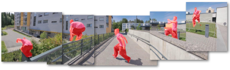
Figure 1: Tukey-inspired segmentation of DAVIS’s Parkour video, which has a moving camera, a dynamic foreground object with scale-variation, and occlusions (best viewed in color).

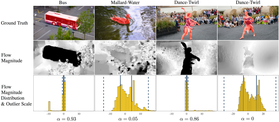
Figure 2: Foreground Candidates in Image Data. The outlier scale $\alpha$ acts as a saliency weighting that adapts to frame-to-frame video characteristics. In these examples, we focus on optical flow magnitude with outliers depicted as black pixels (middle row). Flow distributions are offset from the median (bottom row) and include the interquartile range (solid lines) and outlier thresholds (dotted lines). In the Bus video, the camera follows the bus while the background moves; from the resulting bimodal distribution, we reliably track the bus as a salient flow outlier ($\alpha=0.93$). In Mallard-Water, due to dynamically flowing background elements, the mallard is difficult to track using flow magnitude ($\alpha=0.05$). In Dance-Twirl, $\alpha=0.86$ when the camera is relatively stationary and $\alpha=0$ when the camera is moving.

2 Related Work

Learning-based methods have become commonplace for VOS benchmarks. However, supervised methods require annotated data, which are exceptionally tedious and costly for segmentation. For example, the state-of-the-art OnAVOS [54] has three distinct types of supervision: first, it trains its base network using the ImageNet [10], Microsoft COCO [27], and PASCAL datasets [12]; second, it fine-tunes using the DAVIS dataset [38]; and, third, it requires a user-provided object mask at the beginning of each video. Other DAVIS benchmark leaders, such as OSVOS-S [31], RGMP [34], OSVOS [4], and MSK [37], have similar requirements. To support learning, some researchers develop their own weakly-annotated (FSEG [20]) or synthetic training data (LMP [49]). Other methods require supervision through components, such as features from a previously-trained network (OFL [52]) or a previously-trained boundary detection algorithm (ARP [24, 57]). Finally, some supervised algorithms are not trained, but still need a user-provided mask at runtime [1, 15, 33, 39]. In contrast, our TIS method has no labeling or training requirements. This design constraint supports application areas where user-provided masks are impractical and application-specific datasets for training are unavailable.

Multiple benchmarks are available to evaluate VOS methods [26, 51], including the Densely Annotated VIdeo Segmentation (DAVIS) dataset [38]. DAVIS evaluates VOS methods across many challenge categories, including multiple instances of occlusions, objects leaving view, scale-variation, appearance change, edge ambiguity, camera-shake, interacting objects, and dynamic background (among others); these challenges frequently occur simultaneously. Using our strictly unsupervised TIS method, we achieve a Jaccard measure (or intersect over union) of 67.6 and, using the combinational variant, a Jaccard measure of 74.9, which is a 17% improvement over previous unsupervised results on DAVIS [3, 14, 16, 25, 36, 47, 55, 56].

Primary Contributions

Our primary contribution is a video object segmentation method that utilizes low-level processes without any training or annotation requirements, neither at training or runtime. Our method achieves the highest performance among all known unsupervised methods and higher performance than many supervised methods on the DAVIS video object segmentation benchmark for single objects, which is our focus. We also develop a variant of our initial approach that adaptively combines segmentations from multiple methods, generating new segmentations that achieve the highest DAVIS performance in every category of unsupervised and supervised approaches. We provide source code for the current work at https://github.com/griffbr/TIS.

3 Tukey-Inspired Segmentation

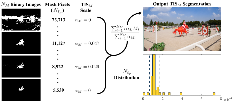
Figure 3: Foreground Objects from Binary Images. In this example, 34 segmentation methods are combined using the TIS_M method (i.e., $N_{M}=34$). The binary image outlier scale $\alpha_{M}$ functions as a confidence weighting for each mask $M$ and changes each video frame. Masks exhibiting a strong $N_{\ell_{p}}$ consensus with the group are considered reliable (middle left), while masks with too many or too few foreground pixels are considered unreliable outliers (top and bottom left, $\alpha_{M}=0$). The $N_{\ell_{p}}$ distribution for the current video frame (bottom right) includes the interquartile range (solid lines) and outlier thresholds (dotted lines).

We derive two Tukey-inspired methods of segmentation. In Section 3.1, we find foreground objects directly from general image data. We identify foreground candidates using John Tukey’s statistical measure of outliers, then we use our own measure of “outlierness” to determine the reliability of each data source for identifying foreground objects. In Section 3.2, we combine a set of binary images that represent previous estimates of foreground object locations, which enables the simultaneous utilization of multiple segmentation methods. To improve accuracy, we use a second “outlierness” measure to determine the reliability of each source segmentation and weight its relative contribution.

3.1 Foreground Candidates in Image Data

Most foreground objects exhibit a measurable difference in data relative to background elements. We identify this difference using outliers in vision data (e.g., optical flow). Given an image $D$ containing data values $d_{p}\in\mathbb{R}$ for each pixel $p$, we calculate lower and upper outlier thresholds:

$${O_{1}}= ~{}{Q_{1}}-k({Q_{3}}-{Q_{1}})$$

$${O_{3}}= ~{}{Q_{3}}+k({Q_{3}}-{Q_{1}}),$$ (1)

where ${Q_{1}}$ and ${Q_{3}}$ are the lower and upper quartiles for all $d_{p}\in D$ and ${Q_{3}}-{Q_{1}}$ is the interquartile range ($Q_{2}$ is the median). $k$ is a constant that scales the outlier thresholds, ${O_{1}}$ and ${O_{3}}$; as suggested by John Tukey in [53], we use $k=1.5$ to find “outliers.” We use each set of outlier data

$$O:=\{d_{p}\in D|d_{p}<{O_{1}}\vee d_{p}>{O_{3}}\}$$ (2)

to identify pixels corresponding to foreground objects.

We also define our own quantitative measure of “outlierness” for each data source $D$:

$$\alpha:=\frac{\sum_{d_{p}\in O}|d_{p}|}{\sum_{d_{p}\in D}|d_{p}|}.$$ (3)

$\alpha\in[0,1]$ is proportional to the magnitude of data in $O$ relative to $D$. By calculating $\alpha$ for each data source, we approximate the frame-to-frame capacity of each source to track foreground objects in a variety of video settings (see Figure 2). Accordingly, we use $\alpha$ to weight each input data source for our example VOS implementation in Section 4.

3.2 Foreground Objects from Binary Images

As an alternative to finding foreground objects in image data, we derive a second outlier scale that enables us to combine segmentation masks from multiple methods and weight their relative contribution according to their frame-to-frame reliability (see Figure 3). Given a set of $N_{M}$ binary masks for the same video frame, assume each mask $M$ consists of pixel-level labels, $\ell_{p}\in\{0,1\}$, where $\ell_{p}=1$ indicates pixel $p$ is a foreground-object location. Compared to image data, the “outlierness” of data within each $M$ is relatively meaningless ($\ell_{p}\in\{0,1\}$ implies that for $\ell_{p}\in M$: $Q_{1},Q_{2},Q_{3}\in\{0,1\}$). Instead, we measure “outlierness” across the set of binary images using the total number of foreground pixels in each $M$,

$$N_{\ell_{p}}:=\sum_{\ell_{p}\in M}\ell_{p}.$$ (4)

Using $N_{\ell_{p}}$, the outlier scale for each mask is defined as

$$\alpha_{M}:=\begin{cases}\text{max}\big{(}~{}\frac{N_{\ell_{p}}-O_{1}}{Q_{2}-O_{1}},0\big{)}&\text{if}~{}N_{\ell_{p}}<Q_{2}\\ \text{max}\big{(}~{}\frac{N_{\ell_{p}}-O_{3}}{Q_{2}-O_{3}},0\big{)}&\text{otherwise}\end{cases},$$ (5)

where quartiles $Q_{1},Q_{2},$ and $Q_{3}$ and thresholds $O_{1}$ and $O_{3}$ are found using (3.1) on the set of $N_{\ell_{p}}$ from all $N_{M}$ masks.

We use $\alpha_{M}\in[0,1]$ to weight each mask based on proximity to the median number of foreground pixels across all $N_{M}$ masks, with outliers being scaled at 0. The intuition behind this weighting is simple. If an individual mask is near the median, it is representative of the collective consensus of segmentation masks for the approximate size of the foreground object, and it is likely more reliable. Alternatively, if an individual mask is an outlier, it is likely unreliable for the current video frame.

To generate the output segmentation mask, we define an image-level estimate of “foregroundness” as

$$F:=\frac{\sum_{i=1}^{N_{M}}\alpha_{M_{i}}M_{i}}{\sum_{i=1}^{N_{M}}\alpha_{M_{i}}},$$ (6)

where $\alpha_{M_{i}}$ is the outlier scale for the $i$th mask $M_{i}$. Note that $F$’s corresponding pixel-level values $f_{p}\in[0,1]$. The final output mask $M$ for the Tukey-inspired combination of binary images is found using

$$\ell_{p}=\begin{cases}1&\text{if}~{}f_{p}>0.5\\ 0&\text{otherwise}\end{cases}.$$ (7)

Remark: In Figure 3 and Section 5.2, we refer to this binary image-based segmentation method as TIS_M.

4 Tukey-Inspired Segmentation using
Motion and Visual Saliency Outliers

We implement the method of finding foreground objects in image data from Section 3.1 using motion and visual saliency data. For motion saliency, $x$ and $y$ optical flow components are found using the method from [29]; in addition, the flow magnitude (i.e., $|x^{2}+y^{2}|$) and flow angle (i.e., $\arctan(\frac{y}{x})$) are also calculated. For each flow measure, the outlier thresholds and scales are calculated on a frame-to-frame basis using (3.1)-(3). The pixel-level motion saliency measure, $d^{\text{ms}}_{p}$, is defined for each flow component as

$$d^{\text{ms}}_{p}:=\begin{cases}0&\text{if}~{}d_{p}\notin O\vee\alpha_{f}<0.5\\ \alpha_{f}|d_{p_{f}}-Q_{2_{f}}|&\text{otherwise}\end{cases},$$ (8)

where $d_{p_{f}}$ is the initial pixel-level flow component value with corresponding frame-to-frame median $Q_{2_{f}}$, outlier scale $\alpha_{f}$, and a 0.5 minimum scale requirement.

The intuition behind (8) is as follows. First, whether a foreground object is moving with a fixed camera or vice versa, the foreground object’s deviation from the frame’s median optical flow will generally be salient (see Bus in Figure 2). Second, the absolute value enables a positive “foregroundness” contribution regardless of a flow component’s sign. Finally, the minimum scale requirement will remove the influence of less reliable flow components.

We found that visual saliency is less useful than optical flow for most video segmentation cases. However, the product of visual saliency and optical flow is beneficial for videos with dynamic background elements (e.g., Mallard-Water in Figure 2). Thus, we include a pixel-level visual saliency measure, $d^{\text{vs}}_{p}$, defined as

$$d^{\text{vs}}_{p}:=({d_{p_{v}}})^{k}\sum_{i=1}^{4}\text{max}(\alpha_{f_{i}},0.5)|d_{p_{f_{i}}}-Q_{2_{f_{i}}}|,$$ (9)

where $d_{p_{v}}\in[0,1]$ is a pixel-level visual saliency-based scale (found using [32]), $k$ is an exponential scale that adjusts the relative sharpness of $({d_{p_{v}}})^{k}\in[0,1]$, $d_{p_{f_{i}}}$ is the $i$th flow component with corresponding median $Q_{2_{f_{i}}}$ and outlier scale $\alpha_{f_{i}}$, and the minimum applied scale of 0.5 ensures that visual saliency features are available even if $\alpha_{f_{i}}=0~{}\forall i$. Three $d^{\text{vs}}_{p}$ measures are used altogether, with $k=\{1,\frac{1}{2},\frac{1}{3}\}$.

To generate the segmentation mask, we combine the four $d^{\text{ms}}_{p}$ and three $d^{\text{vs}}_{p}$ saliency measures for a pixel-level estimate of “foregroundness,” defined as

$$f_{p}:=\sum_{i=1}^{7}d^{i}_{p},$$ (10)

where $d^{i}_{p}$ is the $i$th measure. Using (10), we generate a mask $M$ for each video frame with pixel-level labels

$$\ell_{p}=\begin{cases}1&\text{if}~{}f_{p}>\beta\delta_{p}\\ 0&\text{otherwise}\end{cases},$$ (11)

where $\ell_{p}=1$ indicates a foreground object and $\beta\in\mathbb{R}$ is the sum of the mean and standard deviation of $f_{p}$ in the current frame. $\delta_{p}$ is the pixel-level previous-mask “discount”

$$\delta_{p}:=\begin{cases}\frac{1}{2}&\text{if}~{}\ell_{p,{i}-1}=1\\ 1&\text{otherwise}\end{cases}.$$ (12)

In simple words, if $f_{p}$ is greater than the pixel-level mean and standard deviation of “foregroundness” in the current frame, pixel $p$ is considered a foreground object location. In addition, wherever $p$ corresponds to a mask position in the previous frame, a half-threshold discount is applied, which encourages frame-to-frame continuity and gradually increasing accuracy of the segmentation mask. Finally, the output segmentation mask assumes a single foreground object hypothesis, so the mask in each frame is the single continuous segment with the greatest $f_{p}$ sum.

Remark: In the remainder of the paper, we refer to this image data-based segmentation method as TIS₀.

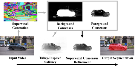
Figure 4: Consensus-based Boundary Refinement. Our Tukey-inspired segmentation (TIS₀) uses saliency outliers in image data to form a quantitative estimate of “foregroundness” and a corresponding object mask. Using supervoxels generated from the input video, we refine TIS₀ with a supervoxel-based consensus for both background and foreground elements, improving the boundary accuracy of the TIS₀ segmentation.

4.1 Consensus-based Boundary Refinement

To improve the boundary accuracy of (11), we use supervoxel consensus voting. This choice is motivated by previous VOS work in [14] that relates the “foregroundness” of superpixels to nearest neighbors across frames. Supervoxels, on the other hand, inherently exist across many frames and have shown promising results for relating features [46, 61] and detecting object boundaries [59]. Given a set of non-overlapping supervoxels that cover all video pixels, we use TIS₀ to build an internal consensus within the bounds of each supervoxel, and then relate this consensus across the video to refine the boundary of the initial TIS₀ mask. This refinement process is depicted in Figure 4.

First, using $\ell_{p}\in\{0,1\}$ from (11), the local consensus within each supervoxel $S$ is defined as

$$f^{\text{L}}_{S}:=\frac{1}{N_{p}}\sum_{p\in S}(2\ell_{p}-1),$$ (13)

where $N_{p}$ is the number of pixels $p\in S$. Note that $f^{\text{L}}_{S}\in[-1,1]$, where positive or negative values imply a foreground object or background.

Next, the non-local consensus among each $S$ is found as

$$f^{\text{NL}}_{S}=\sum_{i=1}^{N_{\text{NL}}}w_{i}f^{\text{L}}_{S_{i}},$$ (14)

where $N_{\text{NL}}$ is the number of nearest-neighbors contributing to the non-local consensus for supervoxel $S$ and $w_{i}$ determines the relative weight of each neighbor. Because the total number of supervoxels, $N_{S}$, changes with each video, we set $N_{\text{NL}}=\lceil\frac{N_{S}}{100}\rceil$. Nearest neighbor weight $w_{i}$ is set as

$$w_{i}=\frac{1}{R(S,S_{i})^{2}},$$ (15)

where $R\in\mathbb{R}$ calculates the city-block distance between the mean-LAB color of local supervoxel $S$ and the $i$th nearest neighbor $S_{i}$. To ensure that all three LAB distances are meaningful, video-wide LAB values are linearly mapped between 0 and 1. $R$ is squared to reduce the influence of supervoxels outside of the primary “clique.”

Finally, to refine the TIS₀ segmentation, we add (13) and (14) to the initial estimate of “foregroundness” from (10):

$$f^{\prime}_{p}:=f_{p}+w_{0}f^{\text{L}}_{S}+f^{\text{NL}}_{S},$$ (16)

where $f^{\text{L}}_{S}$ are $f^{\text{NL}}_{S}$ are the local and non-local consensus for the supervoxel containing $p$ and $w_{0}$ determines the relative weight of $f^{\text{L}}_{S}$ to $f^{\text{NL}}_{S}$. Essentially, $f^{\prime}_{p}$ improves the $f_{p}$-based boundary by adding to supervoxels with a consistent foreground object consensus while subtracting from supervoxels with a consistent background consensus. The refined TIS₀ segmentation mask is found using pixel-level labels

$$\ell_{p}=\begin{cases}1&\text{ if }f^{\prime}_{p}>0\\ 0&\text{otherwise}\end{cases}.$$ (17)

Remarks: (a) $f_{p}$ in (16) is scaled s.t. $f_{p}\in[0,1]$. (b) If using only local consensus, $w_{0}=1$ in (16) and all non-local weights are zeroed. (c) If using local and non-local consensus, $w_{0}=\frac{1}{3}$ and non-local weights are uniformly scaled $s.t.\sum_{i=1}^{N_{\text{NL}}}w_{i}=\frac{2}{3}$. (d) The refined mask (17) is limited to the two segments with the greatest $f^{\prime}_{p}$ sum in each frame. This improves VOS for objects with partial occlusions.

Table 1: DAVIS Results for TIS₀ with and without Supervoxel Consensus Refinement. GBH-based refinement performs better when using only the local consensus. Higher numbers are better for rows labeled with $\uparrow$ (e.g., $\mathcal{J}$ mean) and worse for rows with $\downarrow$.

	Configuration ID
Configuration	TIS${}_{\text{S}}$	TIS${}_{\text{G}}^{\text{L}}$	TIS0
Supervoxels Used	SWA	GBH	None
Hierarchy Level	6	2	N/A
Local Consensus	Yes	Yes	N/A
Non-Local Consensus	Yes	No	N/A
Measure	DAVIS Results
Region Similarity: $\mathcal{J}$ Mean $\uparrow$	67.6	65.3	58.6
Contour Accuracy: $\mathcal{F}$ Mean $\uparrow$	63.9	61.2	47.5
Temporal Stability: $\mathcal{T}$ Mean $\downarrow$	31.0	31.8	30.7

Table 2: Complete DAVIS Results for State-of-the-Art Unsupervised Methods. Methods are unsupervised, so we compare using training and validation videos. Object recall measures the fraction of sequences scoring higher than 0.5, and decay quantifies the performance loss (or gain) over time [38]. TIS₀ exhibits the best decay performance; TIS${}_{\text{S}}$ and TIS_M achieve top results in all other categories.

	Current Results				[56]
Measure	TISM	TIS${}_{\text{S}}$	TIS0	NLC	BGM	FST	KEY	MSG	CVOS	TRC	SAL
Mean $\uparrow$	74.9	67.6	58.6	64.1	62.5	57.5	56.9	54.3	51.4	50.1	42.6
$\mathcal{J}$ Recall $\uparrow$	90.1	84.7	75.9	73.1	70.0	65.2	67.1	63.6	58.1	56.0	38.6
Decay $\downarrow$	5.8	4.0	2.3	8.6	-	4.4	7.5	2.8	12.7	5.0	8.4
Mean $\uparrow$	69.0	63.9	47.5	59.3	59.3	53.6	50.3	52.5	49.0	47.8	38.3
$\mathcal{F}$ Recall $\uparrow$	83.8	78.5	48.8	65.8	66.2	57.9	53.4	61.3	57.8	51.9	26.4
Decay $\downarrow$	9.0	5.7	1.4	8.6	-	6.5	7.9	5.7	13.8	6.6	7.2

Table 3: DAVIS Validation Set Results. Runtime supervision requires a user-provided annotation frame for each segmentation video. Training supervision includes dataset training and dataset-trained components (e.g., OFL and ARP). The online benchmark distinguishes by runtime supervision only. TIS₀-based methods achieve top unsupervised results; TIS_M-based methods achieve top results in all categories.

	Supervision Required
	Runtime & Training							Runtime		Training			Unsuperivsed
Measure	TIS${}_{M5}^{\text{V}}$	TIS${}_{M}^{\text{RTV}}$	OnAVOS	OSVOS-S	CINM	FAVOS	RGMP	TIS${}_{M}^{\text{RV}}$	BVS	TIS${}_{M}^{\text{TV}}$	PDB	ARP	TIS${}_{M}^{V}$	TIS${}_{\text{S}}$	TIS0	FST	CUT
$\mathcal{J}$ Mean	88.1	86.7	86.1	85.6	83.4	82.4	81.5	76.5	60.0	81.8	77.2	76.2	71.2	62.6	56.2	55.8	55.2
$\mathcal{F}$ Mean	87.5	83.8	84.9	87.5	85.0	79.5	82.0	71.2	58.8	76.6	74.5	70.6	66.4	59.6	45.6	51.1	55.2

5 Results

We evaluate our TIS segmentation methods on two VOS benchmark datasets: the Densely Annotated VIdeo Segmentation (DAVIS) dataset [38] and the Georgia Tech Segmentation and Tracking Dataset (SegTrackv2) [26, 51]. The DAVIS 2016 dataset includes 50 diverse videos, 30 training and 20 validation, all of which have ground truth annotations matching the single object hypothesis (unlike DAVIS 2017-18). The SegTrackv2 dataset has fewer videos than DAVIS, and only a subset match the single object hypothesis. SegTrackv2 also contains videos with different resolutions, which span from 76,800 to 230,400 pixels per frame.

Three standard benchmark measures evaluate the performance of our segmentation method: region similarity $\mathcal{J}$, contour accuracy $\mathcal{F}$, and temporal stability $\mathcal{T}$, which are all calculated using the definitions provided in [38]. Region similarity (also known as the intersect over union or Jaccard index [13]) provides an intuitive, scale-invariant evaluation for the number of mislabeled foreground pixels with respect to a ground truth annotation. Given a foreground mask $M$ and ground truth annotation $G$, $\mathcal{J}=\frac{M\cap G}{M\cup G}$. Contour accuracy evaluates the boundary of a segmentation by measuring differences between the closed set of contours for $M$ and $G$. Finally, temporal stability is a measure based on the consistency of a mask between video frames.

Table 4: SegTrackv2 Results. Other results are directly from citation or comparative studies in [14, 20, 62]. Videos are single-object only.

	Unsupervised									Supervised
Video	Current Results				[58]	[62]	[19]
$\mathcal{J}$ Mean	TIS${}^{\text{L}}_{\text{G}}$	TIS${}_{\text{S}}$	TIS0	NLC	ITS	FAM	HPF	KEY	FST	FSEG	HVS
Birdfall	62	54	23	74	73	66	58	49	18	38	57
Frog	78	50	61	83	80	81	58	0	54	57	67
Girl	69	70	65	91	86	82	69	88	55	67	32
Monkey	58	57	34	71	83	69	69	79	65	8	62
Parachute	88	88	67	94	96	90	94	96	76	52	69
Soldier	56	53	49	83	76	83	6	67	4	7	67
Worm	77	58	52	81	82	82	84	84	73	51	35
All	70	62	50	82	82	79	70	66	54	59	56

5.1 TIS₀ Foreground Objects from Image Data

We evaluate our Tukey-inspired measure for finding foreground objects in image data using the TIS₀ implementation from Section 4. To improve boundary accuracy, we refine TIS₀ with supervoxel consensus (Section 4.1) using segmentation by weighted aggregation (SWA) [9, 40] and hierarchical graph-based (GBH) [18] supervoxels (both generated using the LIBSVX library [60]). Both TIS₀ refinement configurations are detailed in Table 1 with additional analysis provided in [17].

DAVIS results for TIS₀-based methods are compared with state-of-the-art methods in Tables 2 and 3. TIS₀ exhibits the best decay performance for $\mathcal{J}$ and $\mathcal{F}$ and achieves a higher $\mathcal{J}$ than all previous unsupervised methods on the DAVIS validation set. Multiple methods have better contour accuracy than TIS₀, but the refinement process from Section 4.1 solves this problem. TIS${}_{\text{S}}$, which improves TIS₀ with consensus-based boundary refinement, outperforms all unsupervised segmentation methods for both $\mathcal{J}$ and $\mathcal{F}$.

SegTrackv2 results are provided in Table 4. We select videos from SegTrackv2 that use a single object hypothesis (like DAVIS). SegTrackv2 uses videos with different resolutions, causing individual hierarchy levels to have dramatically different supervoxel quantities from one video to the next. Accordingly, we change supervoxel hierarchy levels for TIS${}_{\text{S}}$ and TIS${}^{\text{L}}_{\text{G}}$ between videos. Besides NLC, ITS, and FAM, TIS${}^{\text{L}}_{\text{G}}$ achieves top results.

5.2 TIS_M Foreground Objects from Binary Images

Table 5: DAVIS Results for Multiple TIS_M Configurations. Bold font indicates best performance for a given set of methods combined. With the exception of “Experimental Sets,” TIS_M configurations use all applicable methods from the online benchmark (davischallenge.org).

Configuration				Results
ID	Supervised	Methods Combined	Total	$\mathcal{J}$	$\mathcal{F}$
Complete DAVIS Dataset
TISM	No	TIS${}_{\text{S}}$, TIS0, FST[36], NLC[14], MSG[3], KEY[25], CVOS[47], TRC[16]	8	74.9	69.0
TIS${}_{M}^{\text{T}}$	Training	TISM set + ARP[24], FSEG[20], LMP[49]	11	80.5	74.2
TIS${}_{M}^{\text{R}}$	Runtime	TISM set + BVS[33], FCP[39], JMP[15], HVS[18], SEA[8]	13	78.2	73.5
TIS${}_{M}^{\text{RT}}$	R. & T.	TIS${}_{M}^{\text{R}}$ $\cup$ TIS${}_{M}^{\text{T}}$ sets + MSK[37], CTN[22], VPN[21], OFL[52]	20	83.3	78.5
Baseline Comparisons on DAVIS Validation Set
TIS${}_{M}^{\text{V}}$	No	TISM set & CUT[23]	9	71.2	66.4
meanM	No	“                               ”	9	73.3	67.7
medianM	No	“                               ”	9	64.8	60.0
TIS${}_{M}^{\text{TV}}$	Training	TIS${}_{M}^{\text{V}}$ $\cup$ TIS${}_{M}^{\text{T}}$ sets + PDB[42], LVO[50], SFLU[8]	15	81.8	76.6
meanM	Training	“                                                                               ”	15	80.8	75.3
medianM	Training	“                                                                               ”	15	76.0	70.3
TIS${}_{M}^{\text{RV}}$	Runtime	TIS${}_{M}^{\text{V}}$ $\cup$ TIS${}_{M}^{\text{R}}$ sets	14	76.5	71.2
meanM	Runtime	“                            ”	14	76.7	70.8
medianM	Runtime	“                            ”	14	70.3	64.4
TIS${}_{M}^{\text{RTV}}$	R. & T.	TIS${}_{M}^{\text{RT}}$ $\cup$ TIS${}_{M}^{\text{TV}}$ sets + OSVOS-S[31], OnAVOS[54], CINM[2], PML[6],	34	86.7	83.8
		RGMP[34], FAVOS[7], OSVOS[4], SFLS[8], OSMN[63], PLM[41]
meanM	R. & T.	“                                                                                                                ”	34	86.1	82.9
medianM	R. & T.	“                                                                                                                ”	34	80.6	77.1
Experimental Sets on DAVIS Validation Set
TIS${}_{M5}^{\text{V}}$	R. & T.	OSVOS-S, OnAVOS, CINM, RGMP, FAVOS	5	88.1	87.5
meanM	R. & T.	“                                                                      ”	5	88.5	87.7
TIS${}_{M19}^{\text{V}}$	R. & T.	TIS${}_{M5}^{\text{RTV}}$ and TIS${}_{M}^{\text{RV}}$ sets	19	85.8	82.6
meanM	R. & T.	“                                 ”	19	83.8	80.4

We evaluate our Tukey-inspired measure for finding foreground objects in binary images (Section 3.2) by combining the segmentation methods listed in Table 5. Each combination set includes a certain level of supervision: strictly unsupervised (TIS_M), training on an annotated dataset (TIS${}_{M}^{\text{T}}$), user-provided object mask at runtime (TIS${}_{M}^{\text{R}}$), or both user-provided masks and dataset training (TIS${}_{M}^{\text{RT}}$). Some source segmentation methods are only available on the DAVIS Validation Set; TIS_M configurations using these validation methods are only evaluated on the validation set and are distinguished by a V (e.g., TIS${}_{M}^{\text{V}}$).

TIS_M-based methods achieve top DAVIS results for unsupervised segmentation and all categories of supervised segmentation, as shown in Table 3 and Figure 5. For the complete dataset, the relative $\mathcal{J}$ increases over previous results in each category are: 17% for unsupervised (TIS_M to NLC), 6% for training (TIS${}_{M}^{\text{T}}$ to ARP), 18% for runtime (TIS${}_{M}^{\text{R}}$ to BVS), and 4% for runtime and training (TIS${}_{M}^{\text{RT}}$ to MSK). For the validation set, the relative increases are: 28% for unsupervised (TIS${}_{M}^{\text{V}}$ to FST), 6% for training (TIS${}_{M}^{\text{TV}}$ to PDB), 28% for runtime (TIS${}_{M}^{\text{RV}}$ to BVS), and 2% for runtime and training (TIS${}_{M5}^{\text{V}}$ to OnAVOS). The greatest increases for TIS_M combinations over constituent methods occur for categories with a lower $\mathcal{J}$ score (see Figure 5).

To further evaluate TIS_M, we compare against two additional statistics-based methods for combining segmentations. First, we test a mean-based combination (mean_M) that averages all source masks together and outputs a foreground label where the pixel-level mean is higher than 0.5; this is equivalent to setting $\alpha_{M_{i}}=1$ in (6). Second, we test a median-based combination (median_M) that outputs the source mask with the median number of foreground pixels ($N_{\ell_{p}}$ in (4)). For the baseline comparison in Table 5, TIS_M has the highest combined $\mathcal{J}$ and $\mathcal{F}$ score for all categories of supervision but one (mean_M over TIS${}_{M}^{\text{V}}$). In addition, TIS_M is the only combination method that achieves higher $\mathcal{J}$ scores than all source segmentation methods.

Figure 5: Visual Comparison of Segmentation Methods on Complete DAVIS Dataset. Note the correlation between $\mathcal{J}$ and $\mathcal{F}$. The TIS_M segmentation methods improve performance across all categories of supervised and unsupervised methods.

As a final experiment for combining segmentations, we additionally test a small set of the top-five methods (TIS${}_{M5}^{\text{V}}$) and a larger set combining the same top-five methods with many poorer segmentations (TIS${}_{M19}^{\text{V}}$). We postulate that the TIS_M combination method is well-suited for the larger, more variable set of segmentations, where the elimination of poorer-performing outliers and promotion of reliable inliers is critical. This is evidenced by TIS${}_{M19}^{\text{V}}$ and the other large TIS_M sets in Table 5 outperforming mean_M. On the other hand, on a smaller, less variable set of segmentation methods, the calculation of quartiles and outliers for scaling is less meaningful; consequently, we find that the small-set TIS${}_{M5}^{\text{V}}$ and mean_M have similar performance.

6 Discussion and Future Work

We develop a Tukey-inspired segmentation methodology to discover foreground objects in general image data. Our approach automatically adjusts its reliance on each data source according to the frame-to-frame characteristics of a video, addressing a primary challenge in video object segmentation of maintaining reliable measures with changing video characteristics. In addition, our Tukey-inspired measure for finding foreground objects in image data sets a new precedent on the DAVIS dataset for unsupervised segmentation methods. Our current implementation used optical flow and visual saliency data, but the method can incorporate additional sources of image data to accommodate new applications.

We apply a variant of our Tukey-inspired measure to combine the output of other segmentation methods, generating a new and collectively more robust method of segmentation. Our combination method achieves better performance on the DAVIS dataset than all prior segmentation methods and represents a new paradigm in video object segmentation. In real-world applications, it is difficult to know which individual segmentation methods will perform best for various videos. On the other hand, by using our approach, multiple methods can be implemented simultaneously, and only the most reliable methods will be used for segmentation in any given video frame. This extension was particularly effective when constitute methods had variable performance and a large gap for improvement, indicating that the Tukey-inspired combination can be a viable tool for cutting-edge applications where performance has not yet reached its potential. Furthermore, we found that attempting to combine segmentations using “non-Tukey” methods can result in worse performance than some of the source segmentations. Finally, our combination method can easily incorporate new, better-performing segmentation methods as they are developed by the research community.

Given that the current results are restricted to a single object hypothesis, we are currently working on extending this approach to multiple objects. We are also exploring how our method of weighting input data based on “outlierness” can improve performance in supervised learning applications.

References

- [1] S. Avinash Ramakanth and R. Venkatesh Babu. Seamseg: Video object segmentation using patch seams. In Proceedings of the IEEE Conference on Computer Vision and Pattern Recognition (CVPR), 2014.
- [2] L. Bao, B. Wu, and W. Liu. CNN in MRF: video object segmentation via inference in A cnn-based higher-order spatio-temporal MRF. In IEEE Conference on Computer Vision and Pattern Recognition (CVPR), 2018.
- [3] T. Brox and J. Malik. Object segmentation by long term analysis of point trajectories. In European conference on computer vision, pages 282–295. Springer, 2010.
- [4] S. Caelles, K.-K. Maninis, J. Pont-Tuset, L. Leal-Taixé, D. Cremers, and L. Van Gool. One-shot video object segmentation. In IEEE Conference on Computer Vision and Pattern Recognition (CVPR), 2017.
- [5] D.-J. Chen, H.-T. Chen, and L.-W. Chang. Video object cosegmentation. In ACM International Conference on Multimedia, 2012.
- [6] Y. Chen, J. Pont-Tuset, A. Montes, and L. Van Gool. Blazingly fast video object segmentation with pixel-wise metric learning. In Computer Vision and Pattern Recognition (CVPR), 2018.
- [7] J. Cheng, Y.-H. Tsai, W.-C. Hung, S. Wang, and M.-H. Yang. Fast and accurate online video object segmentation via tracking parts. In IEEE Conference on Computer Vision and Pattern Recognition (CVPR), 2018.
- [8] J. Cheng, Y.-H. Tsai, S. Wang, and M.-H. Yang. Segflow: Joint learning for video object segmentation and optical flow. In IEEE International Conference on Computer Vision (ICCV), 2017.
- [9] J. J. Corso, E. Sharon, S. Dube, S. El-Saden, U. Sinha, and A. Yuille. Efficient multilevel brain tumor segmentation with integrated bayesian model classification. IEEE transactions on medical imaging, 27(5):629–640, 2008.
- [10] J. Deng, W. Dong, R. Socher, L. J. Li, K. Li, and L. Fei-Fei. Imagenet: A large-scale hierarchical image database. In IEEE Conference on Computer Vision and Pattern Recognition (CVPR), 2009.
- [11] I. Endres and D. Hoiem. Category Independent Object Proposals, pages 575–588. Springer Berlin Heidelberg, Berlin, Heidelberg, 2010.
- [12] M. Everingham, S. M. A. Eslami, L. Van Gool, C. K. I. Williams, J. Winn, and A. Zisserman. The pascal visual object classes challenge: A retrospective. International Journal of Computer Vision, 111(1):98–136, Jan 2015.
- [13] M. Everingham, L. Van Gool, C. K. Williams, J. Winn, and A. Zisserman. The pascal visual object classes (VOC) challenge. International journal of computer vision, 88(2):303–338, 2010.
- [14] A. Faktor and M. Irani. Video segmentation by non-local consensus voting. In British Machine Vision Conference (BMVC), 2014.
- [15] Q. Fan, F. Zhong, D. Lischinski, D. Cohen-Or, and B. Chen. Jumpcut: non-successive mask transfer and interpolation for video cutout. ACM Trans. Graph., 34(6):195, 2015.
- [16] K. Fragkiadaki, G. Zhang, and J. Shi. Video segmentation by tracing discontinuities in a trajectory embedding. In Computer Vision and Pattern Recognition (CVPR), 2012 IEEE Conference on, pages 1846–1853. IEEE, 2012.
- [17] B. A. Griffin and J. J. Corso. Video object segmentation using supervoxel-based gerrymandering. CoRR, abs/1704.05165, 2017.
- [18] M. Grundmann, V. Kwatra, M. Han, and I. Essa. Efficient hierarchical graph-based video segmentation. In 2010 IEEE Computer Society Conference on Computer Vision and Pattern Recognition, pages 2141–2148, June 2010.
- [19] E. Haller and M. Leordeanu. Unsupervised object segmentation in video by efficient selection of highly probable positive features. In 2017 IEEE International Conference on Computer Vision (ICCV), pages 5095–5103, Oct 2017.
- [20] S. D. Jain, B. Xiong, and K. Grauman. Fusionseg: Learning to combine motion and appearance for fully automatic segmention of generic objects in videos. arXiv preprint arXiv:1701.05384, 2017.
- [21] V. Jampani, R. Gadde, and P. V. Gehler. Video propagation networks. In IEEE Conference on Computer Vision and Pattern Recognition (CVPR), 2017.
- [22] W. D. Jang and C. S. Kim. Online video object segmentation via convolutional trident network. In 2017 IEEE Conference on Computer Vision and Pattern Recognition (CVPR), pages 7474–7483, July 2017.
- [23] M. Keuper, B. Andres, and T. Brox. Motion trajectory segmentation via minimum cost multicuts. In IEEE International Conference on Computer Vision (ICCV), 2015.
- [24] Y. J. Koh and C. S. Kim. Primary object segmentation in videos based on region augmentation and reduction. In 2017 IEEE Conference on Computer Vision and Pattern Recognition (CVPR), pages 7417–7425, July 2017.
- [25] Y. J. Lee, J. Kim, and K. Grauman. Key-segments for video object segmentation. In IEEE International Conference on Computer Vision (ICCV), 2011.
- [26] F. Li, T. Kim, A. Humayun, D. Tsai, and J. M. Rehg. Video segmentation by tracking many figure-ground segments. In The IEEE International Conference on Computer Vision (ICCV).
- [27] T.-Y. Lin, M. Maire, S. Belongie, J. Hays, P. Perona, D. Ramanan, P. Dollár, and C. L. Zitnick. Microsoft coco: Common objects in context. In D. Fleet, T. Pajdla, B. Schiele, and T. Tuytelaars, editors, Computer Vision – ECCV 2014, pages 740–755, Cham, 2014. Springer International Publishing.
- [28] B. Liu and X. He. Multiclass semantic video segmentation with object-level active inference. In IEEE Conference on Computer Vision and Pattern Recognition, 2015.
- [29] C. Liu. Beyond pixels: exploring new representations and applications for motion analysis. PhD thesis, Citeseer, 2009.
- [30] J. Lu, R. Xu, and J. J. Corso. Human action segmentation with hierarchical supervoxel consistency. In IEEE Conference on Computer Vision and Pattern Recognition, 2015.
- [31] K. Maninis, S. Caelles, Y. Chen, J. Pont-Tuset, L. Leal-Taix , D. Cremers, and L. V. Gool. Video object segmentation without temporal information. IEEE Transactions on Pattern Analysis and Machine Intelligence, pages 1–1, 2018.
- [32] R. Margolin, A. Tal, and L. Zelnik-Manor. What makes a patch distinct? In Proceedings of the IEEE Conference on Computer Vision and Pattern Recognition, pages 1139–1146, 2013.
- [33] N. M rki, F. Perazzi, O. Wang, and A. Sorkine-Hornung. Bilateral space video segmentation. In 2016 IEEE Conference on Computer Vision and Pattern Recognition (CVPR), pages 743–751, June 2016.
- [34] S. W. Oh, J.-Y. Lee, K. Sunkavalli, and S. J. Kim. Fast video object segmentation by reference-guided mask propagation. In IEEE Conference on Computer Vision and Pattern Recognition (CVPR), 2018.
- [35] D. Oneata, J. Revaud, J. Verbeek, and C. Schmid. Spatio-temporal object detection proposals. In European Conference on Computer Vision, 2014.
- [36] A. Papazoglou and V. Ferrari. Fast object segmentation in unconstrained video. In Proceedings of the IEEE International Conference on Computer Vision (ICCV), 2013.
- [37] F. Perazzi, A. Khoreva, R. Benenson, B. Schiele, and A.Sorkine-Hornung. Learning video object segmentation from static images. In IEEE Conference on Computer Vision and Pattern Recognition (CVPR), 2017.
- [38] F. Perazzi, J. Pont-Tuset, B. McWilliams, L. Van Gool, M. Gross, and A. Sorkine-Hornung. A benchmark dataset and evaluation methodology for video object segmentation. In IEEE Conference on Computer Vision and Pattern Recognition (CVPR), 2016.
- [39] F. Perazzi, O. Wang, M. Gross, and A. Sorkine-Hornung. Fully connected object proposals for video segmentation. In IEEE International Conference on Computer Vision (ICCV), 2015.
- [40] E. Sharon, M. Galun, D. Sharon, R. Basri, and A. Brandt. Hierarchy and adaptivity in segmenting visual scenes. Nature, 442(7104):810–813, 2006.
- [41] J. Shin Yoon, F. Rameau, J. Kim, S. Lee, S. Shin, and I. So Kweon. Pixel-level matching for video object segmentation using convolutional neural networks. In IEEE International Conference on Computer Vision (ICCV), 2017.
- [42] H. Song, W. Wang, S. Zhao, J. Shen, and K.-M. Lam. Dilated pyramid convolution and deeper bidirectional convlstm for video salient object detection. In The European Conference on Computer Vision (ECCV), September 2018.
- [43] K. Soomro, H. Idrees, and M. Shah. Action localization in videos through context walk. In IEEE International Conference on Computer Vision, 2015.
- [44] K. Soomro, H. Idrees, and M. Shah. Predicting the where and what of actors and actions through online action localization. In IEEE Conference on Computer Vision and Pattern Recognition, 2016.
- [45] K. Tang, R. Sukthankar, J. Yagnik, and L. Fei-Fei. Discriminative segment annotation in weakly labeled video. In IEEE Conference on Computer Vision and Pattern Recognition, 2013.
- [46] E. H. Taralova, F. De la Torre, and M. Hebert. Motion words for videos. In European Conference on Computer Vision, pages 725–740. Springer, 2014.
- [47] B. Taylor, V. Karasev, and S. Soatto. Causal video object segmentation from persistence of occlusions. In Proceedings of the IEEE Conference on Computer Vision and Pattern Recognition, pages 4268–4276, 2015.
- [48] J. Tighe and S. Lazebnik. Superparsing: scalable nonparametric image parsing with superpixels. International Journal of Computer Vision, 2012.
- [49] P. Tokmakov, K. Alahari, and C. Schmid. Learning motion patterns in videos. In 2017 IEEE Conference on Computer Vision and Pattern Recognition (CVPR), pages 531–539, July 2017.
- [50] P. Tokmakov, K. Alahari, and C. Schmid. Learning video object segmentation with visual memory. In IEEE International Conference on Computer Vision (ICCV), 2017.
- [51] D. Tsai, M. Flagg, A. Nakazawa, and J. M. Rehg. Motion coherent tracking using multi-label mrf optimization. International journal of computer vision, 100(2):190–202, 2012.
- [52] Y. H. Tsai, M. H. Yang, and M. J. Black. Video segmentation via object flow. In 2016 IEEE Conference on Computer Vision and Pattern Recognition (CVPR), pages 3899–3908, June 2016.
- [53] J. W. Tukey. Exploratory data analysis. 1977.
- [54] P. Voigtlaender and B. Leibe. Online adaptation of convolutional neural networks for video object segmentation. In British Machine Vision Conference (BMVC), 2017.
- [55] W. Wang, J. Shen, and F. Porikli. Saliency-aware geodesic video object segmentation. In Proceedings of the IEEE Conference on Computer Vision and Pattern Recognition, pages 3395–3402, 2015.
- [56] S. Wehrwein and R. Szeliski. Video segmentation with background motion models. In British Machine Vision Conference (BMVC), 2017.
- [57] P. Weinzaepfel, J. Revaud, Z. Harchaoui, and C. Schmid. Learning to detect motion boundaries. In 2015 IEEE Conference on Computer Vision and Pattern Recognition (CVPR), pages 2578–2586, June 2015.
- [58] F. Xiao and Y. J. Lee. Track and segment: An iterative unsupervised approach for video object proposals. In 2016 IEEE Conference on Computer Vision and Pattern Recognition (CVPR), pages 933–942, June 2016.
- [59] C. Xu and J. J. Corso. Evaluation of super-voxel methods for early video processing. In Computer Vision and Pattern Recognition (CVPR), 2012 IEEE Conference on, pages 1202–1209. IEEE, 2012.
- [60] C. Xu and J. J. Corso. Libsvx: A supervoxel library and benchmark for early video processing. International Journal of Computer Vision, 119(3):272–290, 2016.
- [61] C. Xu, S. Whitt, and J. J. Corso. Flattening supervoxel hierarchies by the uniform entropy slice. In The IEEE International Conference on Computer Vision (ICCV), December 2013.
- [62] J. Yang, B. Price, X. Shen, Z. Lin, and J. Yuan. Fast appearance modeling for automatic primary video object segmentation. IEEE Transactions on Image Processing, 25(2):503–515, Feb 2016.
- [63] L. Yang, Y. Wang, X. Xiong, J. Yang, and A. K. Katsaggelos. Efficient video object segmentation via network modulation. IEEE Conference on Computer Vision and Pattern Recognition (CVPR), 2018.