Gravitational Decoupled Anisotropic Solutions in $f(\mathcal{G})$ Gravity

Abstract

In this paper, we investigate anisotropic static spherically symmetric solutions in the framework of $f(\mathcal{G})$ gravity through gravitational decoupling approach. For this purpose, we consider Krori and Barua (known solution) isotropic interior solution for static spherically symmetric self-gravitating system and extend it to two types of anisotropic solutions. We examine the physical viability of our models through energy conditions, squared speed of sound and anisotropy parameter. It is found that the first solution is physically viable as it fulfills the energy bounds as well as stability criteria while the second solution satisfies all energy bounds but is unstable at the core of the compact star.

Keywords: Anisotropy; $f(\mathcal{G})$ gravity; Gravitational decoupling; Exact solutions.
PACS: 04.20.J.b; 04.40.-b; 98.80.-k; 04.50.Kd.

1 Introduction

Modified theories of gravity have secured extensive recognition after the innovative cosmological aspects of the expanding universe. This intriguing approach is considered as the most promising and optimistic to unveil the hidden characteristics of cosmos. Nojiri and Odintsov [1] introduced modified Gauss-Bonnet gravity (or $f(\mathcal{G})$ gravity) by including higher order correction terms through Gauss-Bonnet (GB) invariant. The motivation behind this theory comes from string theory at low energy scales which is expected to analyze effectively the late-time cosmic transitions. The GB invariant is a four-dimensional topological term which is a combination of the Ricci scalar ($R$), Ricci ($R_{\alpha\beta}$) and Riemann tensors ($R_{\alpha\beta\mu\nu}$), given by $\mathcal{G}=R^{2}-4R_{\alpha\beta}R^{\alpha\beta}+R_{\alpha\beta\mu\nu}R^{\alpha\beta\mu\nu}$. This second Lovelock scalar trivially contributes when included in matter Lagrangian but excludes spin-2 ghost instability [2]. Bamba et al. [3] explored modified $f(\mathcal{G})$ as well as $f(R,\mathcal{G})$ models with some emergent ingredients of finite-time future singularities and investigated higher-order curvature corrections to cure these singularities.

The formulation of appropriate spherically symmetric interior solution of self-gravitating system has always been problematic due to the presence of nonlinearity in the field equations. A plenty of work has been done in literature to tackle this issue. Mak and Harko [4] obtained exact anisotropic solution of the field equations and found the positively finite behavior of density and pressure supporting the core of stellar objects. Gleiser and Dev [5] investigated algorithm of anisotropic self-gravitating system with compactness $\frac{M}{R}=\frac{4}{9}$ and obtained stable model for small measures of adiabatic index. Sharma and Maharaj [6] explored some anisotropic spherical exact solutions in the framework of linear combination of equation of state defining compactness of stellar objects. Kalam et al. [7] found compact models in the context of anisotropic regime using Karori and Barua metric. Bhar et al. [8] discussed the possibilities of existence of compact objects in higher dimensions. Maurya et al. [9] studied anisotropic solutions of compact stars in the presence of charge distribution.

The existence of exact interior solutions of self-gravitating systems in the presence of anisotropy have been carried out in a number of ways. In this regard, the minimal gravitational decoupling (MGD) approach appeared as significantly deterministic in finding the physically viable solutions for spherically symmetric stellar configuration. Ovalle [10] proposed this technique to extract some exact solutions for compact stellar objects in the framework of braneworld. The MGD approach is not a novel idea, indeed some ingredients make it specifically more attractive for searching new spherically symmetric solutions of the Einstein field equations. The main and foremost feature of this technique is that a simple solution can be extended into more complex domains. This technique could be started with a simple source ($T^{(m)}_{\mu\nu}$) in which another gravitational source ($T^{\ast}_{\mu\nu}$) can be added through a coupling constant $\alpha$, i.e., $T^{(m)}_{\mu\nu}\rightarrow\tilde{T}^{(tot)}_{\mu\nu}=T^{(m)}_{\mu\nu}+\alpha T^{\ast}_{\mu\nu}$ such that the spherical symmetry remains preserved. The reverse of this technique also works through de-coupling of gravitationally sources. In order to find the solution of highly non-linear field equations with complex spherically symmetric gravitational sources, we split the source in simple components and find the solution for each of them. This leads to as many solutions as the number of components whose combination will yield the solution of the field equation corresponding to the original energy-momentum tensor. This technique provides a breakthrough in the search of anisotropic solutions extended from isotropic ones.

In this context, Ovalle and Linares [11] formulated an exact solution of the field equations for spherically symmetric isotropic compact distribution and concluded that their results present the braneworld form of Tolman-IV solution. Casadio et al. [12] developed some exterior solutions for spherically symmetric self-gravitating system using gravitational decoupling technique and found naked singularity at Schwarzschild radius. Ovalle [13] decoupled gravitational source to obtain anisotropic solutions from spherically symmetric isotropic solutions. Ovalle et al. [14] extended the isotropic solution by inclusion of anisotropy using MGD approach for static regime of stellar objects. Sharif and Sadiq [15] explored charged anisotropic spherical solution through this approach and also examined the viability conditions, stability criteria through squared speed of sound.

Compact stars being the relativistic massive objects (small size and extremely massive structure) possess very strong gravitational force which can be studied in modified theories of gravity. The curiosity to know more about compact stars brings in many researchers on the platform of modified theories of gravity. Zubair and Abbas [16] investigated the possibilities of formulation of compact star in $f(R)$ gravity using Karori and Barua solution. Abbas and his collaborators [17] analyzed the anisotropic compact star solution in $f(T)$ gravity and examined the surface redshift, stability as well as regularity conditions. Abbas et al. [18] analyzed the anisotropic compact star in $f(\mathcal{G})$ gravity and examined physical behavior of star with observational data. Sharif and Fatima [19] explored static spherically symmetric solutions in $f(\mathcal{G})$ gravity for both isotropic and anisotropic matter distributions.

In this paper, we explore anisotropic spherically symmetric solutions using MGD approach. The paper is organized in the following format. In the next section, we discuss some basic terminologies of $f(\mathcal{G})$ gravity and corresponding field equations for multiple sources. Section 3 is devoted to MGD approach and corresponding junction conditions. In section 4, we find exact anisotropic solutions using some constraints and check their physical behavior. Finally, we conclude our results in the last section.

2 Fluid Configuration and Field Equations for Multiple Sources

The standard field equation for $f(\mathcal{G})$ gravity are [20]

$$R_{\rho\gamma}-\frac{1}{2}Rg_{\rho\gamma}=\kappa T_{\rho\gamma}^{(tot)},$$ (1)

where $\kappa$ is coupling constant with

$$T_{\rho\gamma}^{(tot)}=T_{\rho\gamma}^{(m)}+T_{\rho\gamma}^{(\mathcal{G})}+\alpha\Theta_{\rho\gamma}.$$ (2)

The energy-momentum tensor for perfect fluid configuration containing four-velocity field, density and pressure is

$$T_{\rho\gamma}^{(m)}=(\rho+P)U_{\rho}U_{\gamma}+Pg_{\rho\gamma},$$ (3)

and

$$T_{\rho\gamma}^{(\mathcal{G})} = \frac{1}{2\kappa}g_{\rho\gamma}f(\mathcal{G})+\frac{1}{\kappa}[(4R_{\gamma\mu}R^{\mu}_{\rho}-2RR_{\rho\gamma}-2R_{\rho\mu\eta\nu}R^{\mu\eta\nu}_{\gamma}-4R_{\rho\mu\eta\gamma}R^{\mu\eta})f_{\mathcal{G}}(\mathcal{G})$$ (4)

$$+ (4R_{\rho\gamma}-2Rg_{\rho\gamma})\nabla^{2}f_{\mathcal{G}}(\mathcal{G})+2R\nabla_{\rho}\nabla_{\gamma}f_{\mathcal{G}}(\mathcal{G})$$

$$- 4R_{\rho}^{\mu}\nabla_{\gamma}\nabla_{\mu}f_{\mathcal{G}}(\mathcal{G})-4R_{\gamma}^{\mu}\nabla_{\rho}\nabla_{\mu}f_{\mathcal{G}}(\mathcal{G})$$

$$+ 4g_{\rho\gamma}R^{\mu\eta}\nabla_{\mu}\nabla_{\eta}f_{\mathcal{G}}(\mathcal{G})-4R_{\rho\mu\gamma\eta}\nabla^{\mu}\nabla^{\eta}f_{\mathcal{G}}(\mathcal{G})],$$

where $\nabla^{2}=\nabla_{\mu}\nabla^{\mu}$ ($\nabla_{\mu}$ denotes covariant derivative) is d’Alembert operator and $f_{\mathcal{G}}(\mathcal{G})$ represents derivative of generic function with respect to $\mathcal{G}$. The term $\Theta_{\rho\gamma}$ describes an additional source coupling the gravity through constant $\alpha$ [21] which may incorporate new fields (like scalar, vector or tensor fields) and will produce anisotropy in self-gravitating systems.

The line element of static spherically symmetric spacetime reads

$$ds^{2}=-e^{\eta(r)}dt^{2}+e^{\psi(r)}dr^{2}+r^{2}(d\theta^{2}+\sin^{2}\theta d\phi^{2}),$$ (5)

where $\eta=\eta(r)$, $\psi=\psi(r)$ denote the function of areal radius $r$ ranging from core to the surface of star while $U^{\mu}=e^{-\frac{\eta}{2}}\delta^{\mu}_{0}$ for $0<r<R$. The field equations (1) with (5) yield

$$\kappa(\rho-T_{0}^{0(\mathcal{G})}-\alpha\Theta_{0}^{0}) = \frac{1}{r^{2}}+(\frac{\psi^{\prime}}{r}-\frac{1}{r^{2}})e^{-\psi(r)},$$ (6)

$$\kappa(P+T_{1}^{1(\mathcal{G})}+\alpha\Theta_{1}^{1}) = -\frac{1}{r^{2}}+(\frac{\eta^{\prime}}{r}+\frac{1}{r^{2}})e^{-\psi(r)},$$ (7)

$$\kappa(P+T_{2}^{2(\mathcal{G})}+\alpha\Theta_{2}^{2}) = (\frac{\eta^{\prime}}{2r}+\frac{\eta^{\prime\prime}}{2}+\frac{\eta^{\prime 2}}{4}-\frac{\eta^{\prime}\psi^{\prime}}{4}-\frac{\psi^{\prime}}{2r})e^{-\psi(r)},$$ (8)

where $T_{0}^{0(\mathcal{G})}$, $T_{1}^{1(\mathcal{G})}$ and $T_{2}^{2(\mathcal{G})}$ are given in appendix A. The expression for GB invariant takes the form

$$\mathcal{G}=\frac{2e^{-2\psi}}{r^{2}}[(\eta^{\prime 2}+2\eta^{\prime\prime})(1-e^{\psi})+\eta^{\prime}\psi^{\prime}(e^{\psi})],$$ (9)

where prime denotes the derivative with respect to $r$. The corresponding conservation equation reads

$$\frac{dP}{dr} + \frac{dT_{1}^{1(\mathcal{G})}}{dr}+\alpha\frac{d\Theta_{1}^{1}}{dr}+\frac{\eta^{\prime}}{2}(\rho+P+T_{1}^{1(\mathcal{G})}-T_{0}^{0(\mathcal{G})})+\frac{2}{r}(T_{1}^{1(\mathcal{G})}-T_{2}^{2(\mathcal{G})})$$ (10)

$$+ \frac{\alpha\eta^{\prime}}{2}(\Theta_{1}^{1}-\Theta_{0}^{0})+\frac{2\alpha}{r}(\Theta_{1}^{1}-\Theta_{2}^{2})=0.$$

It is found that the system of non-linear differential equations ((6)-(10)) consists of seven unknown functions ($\psi$, $\eta$, $\rho$, $P$, $\Theta_{0}^{0}$, $\Theta_{1}^{1}$, $\Theta_{2}^{2}$). We adopt systematic approach of Ovalle [14] to determine these unknowns. For the system ((6)-(10)), the matter contents (effective density, effective isotropic pressure and effective tangential pressure) can be identified as

$$\bar{\rho}=\rho-\alpha\Theta_{0}^{0},\quad\bar{P}_{r}=P+\alpha\Theta_{1}^{1},\quad\bar{P}_{t}=P+\alpha\Theta_{2}^{2}.$$ (11)

This clearly shows that the source $\Theta_{\rho\gamma}$ can, in general, bring in anisotropy $\bar{\Delta}=\bar{P}_{t}-\bar{P}_{r}=\alpha(\Theta_{2}^{2}-\Theta_{1}^{1})$ into the inner of stellar distribution.

3 Gravitational Decoupling by MGD Approach

In this section, we use MGD approach to find solution of the system ((6)-(10)) by transforming the field equations such that the source $\Theta_{\rho\gamma}$ takes the form of effective equations which might incorporate anisotropy. Let us consider the perfect fluid solution ($\psi$, $\eta$, $\rho$, $P$) with $\alpha=0$ using line element

$$ds^{2}=-e^{\chi(r)}dt^{2}+\frac{dr^{2}}{\xi(r)}+r^{2}(d\theta^{2}+\sin^{2}\theta d\phi^{2}),$$ (12)

where $\xi(r)=1-\frac{2m}{r}$ contains the Misner-Sharp mass “$m$” for the fluid configuration. We take the effects of source $\Theta_{\rho\gamma}$ in isotropic model by encoding the geometrical deformation undertaken by perfect fluid metric (12) as [14]

$$\chi\rightarrow\eta=\chi+\alpha f,\quad\xi\rightarrow e^{-\psi}=\xi+\alpha h,$$ (13)

where $f$ and $h$ are geometrical deformations offered to temporal and radial metric ingredients. The possibly minimal geometric deformation among aforementioned deformations is

$$f\rightarrow 0,\quad h\rightarrow h^{\ast},$$ (14)

where the radial metric component endures deformation while the temporal component remains the same. Hence the minimal geometric deformation equation (14) turns out to be

$$\chi\rightarrow\eta=\chi,\quad\xi\rightarrow e^{-\psi}=\xi+\alpha h^{\ast},$$ (15)

where $h^{\ast}$ is the deformation function associated to radial metric component. Using Eq.(15), the system ((6)-(10)) splits up into two sets.

The first set gives

$$\kappa(\rho-T_{0}^{0(\mathcal{G})}) = \frac{1}{r^{2}}-(\frac{\xi^{\prime}}{r}+\frac{\xi}{r^{2}}),$$ (16)

$$\kappa(P+T_{1}^{1(\mathcal{G})}) = -\frac{1}{r^{2}}+(\frac{\chi^{\prime}}{r}+\frac{1}{r^{2}})\xi(r),$$ (17)

$$\kappa(P+T_{2}^{2(\mathcal{G})}) = (\frac{\chi^{\prime}}{2r}+\frac{\chi^{\prime\prime}}{2}+\frac{\chi^{\prime 2}}{4})\xi(r)+(\frac{\chi^{\prime}}{4}+\frac{1}{2r})\xi^{\prime}(r),$$ (18)

and the second one containing the source is

$$\kappa\Theta_{0}^{0} = \frac{h^{\ast^{\prime}}}{r}+\frac{h^{\ast}}{r^{2}},$$ (19)

$$\kappa\Theta_{1}^{1} = h^{\ast}(\frac{\chi^{\prime}}{r}+\frac{1}{r^{2}}),$$ (20)

$$\kappa\Theta_{2}^{2} = (\frac{\chi^{\prime}}{2r}+\frac{\chi^{\prime\prime}}{2}+\frac{\chi^{\prime 2}}{4})\xi(r)+(\frac{\chi^{\prime}}{4}+\frac{1}{2r})\xi^{\prime}(r),$$ (21)

The above system (19)-(21) looks similar to the spherically symmetric field equations for anisotropic fluid configuration with source $\Theta_{\rho\gamma}$ ($\rho=-\Theta_{0}^{0},~{}P_{r}=\Theta_{1}^{1},~{}P_{t}=\Theta_{2}^{2}$) corresponding to the metric

$$ds^{2}=-e^{\chi(r)}dt^{2}+\frac{dr^{2}}{h^{\ast}(r)}+r^{2}(d\theta^{2}+\sin^{2}\theta d\phi^{2}).$$ (22)

However, the right-hand side of system (19)-(21) deviates from the anisotropic solution by term $\frac{1}{r^{2}}$ which constitutes the effective matter components as

$$\bar{\rho}=\Theta_{0}^{0\ast}=\Theta_{0}^{0}-\frac{1}{\kappa r^{2}},\quad\bar{P}_{r}=\Theta_{1}^{1\ast}=\Theta_{1}^{1}-\frac{1}{\kappa r^{2}},\quad\bar{P}_{t}=\Theta_{2}^{2\ast}=\Theta_{2}^{2}.$$ (23)

The junction conditions provide smooth matching of interior and exterior geometries at the surface of the stellar object to investigate some significant features of their evolution. For instance, the interior spacetime geometry of stellar distribution is obtained through MGD as

$$ds^{2}=-e^{\eta_{-}(r)}dt^{2}+(1-\frac{2\bar{m}}{r})^{-1}dr^{2}+r^{2}(d\theta^{2}+\sin^{2}\theta d\phi^{2}),$$ (24)

where the interior mass is $\bar{m}=m(r)-\frac{r}{2}\alpha h^{\ast}$. Consider the general exterior metric as

$$ds^{2}=-e^{\eta_{+}(r)}dt^{2}+e^{\psi_{+}(r)}dr^{2}+r^{2}(d\theta^{2}+\sin^{2}\theta d\phi^{2}).$$ (25)

The continuity of the first fundamental form of matching conditions, i.e., $[ds^{2}]_{\Sigma}=0$ ($\Sigma$ is hypersurface or star’s surface ($r=R$)) yields

$$\eta_{+}(R)=\eta_{-}(R),\quad 1-\frac{2M_{0}}{R}+\alpha h^{\ast}(R)=e^{\psi_{+}(R)}.$$ (26)

Similarly, the continuity of second fundamental form ($[G_{\rho\gamma}t^{\gamma}]_{\Sigma}=0$, where $t^{\gamma}$ is a unit four-vector in radial direction) leads to

$$P_{R}+\alpha(\Theta_{1}^{1}(R))^{-}+(T_{1}^{1(\mathcal{G})}(R))^{-}=\alpha(\Theta_{1}^{1}(R))^{+}+(T_{1}^{1(\mathcal{G})}(R))^{+}.$$ (27)

Using the matching condition (26), we obtain $(T_{1}^{1(\mathcal{G})}(R))^{-}=(T_{1}^{1(\mathcal{G})}(R))^{+}$ which implies that

$$P_{R}+\alpha(\Theta_{1}^{1}(R))^{-}=\alpha(\Theta_{1}^{1}(R))^{+},$$ (28)

yielding

$$P_{R}+\frac{\alpha h^{\ast}}{\kappa}(\frac{\eta^{\prime}}{R}+\frac{1}{R^{2}})=\frac{\alpha f^{\ast}}{\kappa R^{2}}(\frac{R}{R-2M}),$$ (29)

where $f^{\ast}=0$ is the outer radial geometric deformation for Schwarzschild metric given as

$$ds^{2}=-(1-\frac{2m}{r})dt^{2}+(1-\frac{2m}{r}+\alpha h^{\ast})^{-1}dr^{2}+r^{2}(d\theta^{2}+\sin^{2}\theta d\phi^{2}).$$ (30)

The necessary and sufficient conditions for smooth matching of MGD interior and exterior Schwarzschild metrics (filled by the field of the source $\Theta_{\rho\gamma}$) are given by the constraints Eqs.(26)-(29). If the exterior geometric metric is taken as the standard Schwarzschild metric ($f^{\ast}=0$) then

$$\bar{P}_{R}=P_{R}+\frac{\alpha h^{\ast}}{\kappa}(\frac{\eta^{\prime}}{R}+\frac{1}{R^{2}})=0.$$ (31)

In the following, we take a known isotropic spherically symmetric solution for our systematic analysis.

4 Interior Solutions

In order to obtain anisotropic solution using MGD decoupling, it is important to find out perfect fluid spherically symmetric solution. In particular, we choose Krori and Barua solution for physical relevance as [22]

$$e^{\eta} = e^{Br^{2}+C},$$ (32)

$$e^{\chi} = \xi^{-1}(r)=e^{Ar^{2}},$$ (33)

$$\rho = \frac{e^{-Ar^{2}}}{\kappa r^{2}}(e^{Ar^{2}}+2Ar^{2}-1)+T_{0}^{0(\mathcal{G})},$$ (34)

$$P = \frac{e^{-Ar^{2}}}{\kappa r^{2}}(-e^{Ar^{2}}+2Br^{2}+1)-T_{1}^{1(\mathcal{G})},$$ (35)

where $A$, $B$ and $C$ are constants that can be derived through matching conditions. The rationale for the aforementioned solution is its singularity-free feature which satisfies physical conditions inside the spherical distribution. For exterior geometric configuration as Schwarzschild metric, the junction condition yields

$$A = -\frac{1}{R^{2}}\ln(1-\frac{2M_{0}}{R}),\quad B=\frac{M_{0}}{R^{2}(R-2M_{0})},$$ (36)

$$C = \ln(\frac{R-2M_{0}}{R})-\frac{M_{0}}{R-2M_{0}},$$ (37)

with compactness $\frac{M_{0}}{R}<\frac{4}{9}$ ($M_{0}$ is the total mass). The above expressions through the matching conditions ensure the continuity of the interior and exterior regions at the boundary of the star which definitely will vary in the presence of source $\Theta_{\rho\gamma}$.

Now, we evaluate anisotropic solution, i.e., $\alpha\neq 0$ in the interior spherical distribution. The temporal and radial metric contents are given by Eqs.(15) and (32) whereas the geometric deformation and source are connected through Eqs.(19)-(21). For this purpose, various choices can be considered such as the equation of state, some particular forms of density as well as pressure or some physically motivated restrictions on $h^{\ast}$ [14, 15, 23]. In any case, we need to remain concerned with physical acceptability of the solution. In the following, we address this problem by taking some conditions to generate physically acceptable interior solutions.

4.1 Solution-I

Herein, we apply the constraint on source component $\Theta_{1}^{1}$ and solve the field equations for deformation function $h^{\ast}$ and source $\Theta_{\rho\gamma}$. One can observe that the exterior geometry of Schwarzschild metric is compatible with interior matter configuration as long as $P+T_{1}^{1(\mathcal{G})}\sim\alpha(\Theta_{1}^{1}(R))_{-}$. The simplest choice which satisfies this crucial requirement is

$$\alpha\Theta_{1}^{1}=P+T_{1}^{1(\mathcal{G})}\quad\Rightarrow\quad h^{\ast}=\xi-\frac{1}{1+r\eta^{\prime}},$$ (38)

where we have used Eqs.(17) and (20). Equation (38) mimics the radial metric component as

$$e^{-\psi}=(1+\alpha)\xi-\frac{\alpha}{1+2Br^{2}}.$$ (39)

The interior geometric component in Eqs.(33) and (39) represent minimally deformed Krori and Barua solution by generic anisotropic source $\Theta_{\rho\gamma}$. In the limit $\alpha\rightarrow 0$, Eq.(39) yields standard isotropic spherical solutions ((32)-(35)).

The continuity of first fundamental form of junction conditions gives

$$Br^{2}+C=\ln(1-\frac{2M}{R}),$$ (40)

$$1-\frac{2M}{R}=(1+\alpha)\xi-\frac{\alpha}{1+2BR^{2}},$$ (41)

whereas the continuity of second fundamental form ($P(R)+T_{1}^{1(\mathcal{G})}+\alpha(\Theta_{1}^{1}(R))_{-}=0$) reads

$$P(R)+T_{1}^{1(\mathcal{G})}=0\Rightarrow A=\frac{\ln(1+2BR^{2})}{R^{2}},$$ (42)

where expression in (38) has been utilized. Using Eq.(41), the Schwarzschild mass is obtained as

$$\frac{2M}{R}=\frac{2(1+\alpha)M_{0}}{R}+\frac{\alpha}{1+2BR^{2}}-\alpha.$$ (43)

Using this in Eq.(40), we have

$$BR^{2}+C=\ln((1+\alpha)(1-\frac{2M_{0}}{R})-\frac{\alpha}{1+2BR^{2}}),$$ (44)

where the constant $C$ is expressed in terms of $B$. Equations (42)-(44) give the necessary and sufficient conditions for smooth matching of interior and exterior spacetimes on the surface of star. Using the mimic constraint (38), the anisotropic solution ($\bar{\rho},\bar{P}_{r},\bar{P}_{t}$) is given by

$$\bar{\rho} = \frac{1}{\kappa(r+2Br^{3})^{2}}[(1+2(1+\alpha)Ar^{2}e^{-Ar^{2}}+(1-\alpha)e^{-Ar^{2}}+\kappa r^{2}T_{0}^{0(\mathcal{G})})$$ (45)

$$\times (1+4Br^{2}(1+Br^{2}))+\alpha(1-2Br^{2})],$$

$$\bar{P}_{r} = \frac{1}{\kappa r^{2}}(1+\alpha)((2Br^{2}+1)e^{-Ar^{2}}-1+\kappa r^{2}T_{1}^{1(\mathcal{G})}),$$ (46)

$$\bar{P}_{t} = \frac{1}{\kappa(r+2Br^{3})^{2}}[\alpha Ar^{2}e^{-Ar^{2}}(1+5Br^{2}+8B^{2}r^{4}+4b^{3}r^{6})+Br^{2}e^{-Ar^{2}}$$ (47)

$$\times (-2(3+\alpha)+3Br^{2}(3\alpha-4)-4B^{2}r^{4}(2+3\alpha)-4\alpha B^{3}r^{6})+\alpha B^{2}r^{4}$$

$$\times (3+2Br^{2})-e^{-Ar^{2}}+(1+\kappa r^{2}T_{1}^{1(\mathcal{G})})(1+4Br^{2}+4B^{2}r^{4})],$$

$$\bar{\Delta} = \bar{P}_{t}-\bar{P}_{r}=\frac{1}{\kappa(r+2Br^{3})^{2}}[1+e^{-Ar^{2}}(-1-Ar^{2}(1+5Br^{2}+8B^{2}r^{4}$$ (48)

$$+ 4B^{3}r^{6})+Br^{2}(-4-3Br^{2}+4B^{2}r^{4}+4B^{3}r^{6}))+B^{2}r^{4}+4Br^{2}$$

$$- 2B^{3}r^{6}+\kappa T_{1}^{1(\mathcal{G})}r^{2}(1+4Br^{2}+4B^{2}r^{4})].$$

4.2 Solution-II

In this case, we take another choice of mimic constraint on density for physically acceptable solution. This constraint ($\alpha\Theta_{0}^{0}\sim\rho-T_{0}^{0(\mathcal{G})}$) implies that

$$h^{\ast}=\frac{c_{1}}{r}+e^{-Ar^{2}}-1,$$ (49)

where $c_{1}$ is the integration constant. By adopting the same methodology as prescribed in solution-I, we obtain the junction conditions as

$$\alpha R(e^{-AR^{2}}-1)+\alpha c_{1}+2(M-M_{0})=0,$$ (50)

$$BR^{2} + C=\ln(1-\frac{2M_{0}}{R}+\frac{\alpha c_{1}}{R}+\alpha(e^{-AR^{2}}-1),$$ (51)

The anisotropic solution satisfying the above matching condition becomes

$$\bar{\rho} = (1-\alpha)[\frac{e^{-Ar^{2}}}{\kappa r^{2}}(e^{Ar^{2}}+2Ar^{2}-1)+T_{0}^{0(\mathcal{G})}],$$ (52)

$$\bar{P}_{r} = \frac{1}{\kappa r^{3}}[2Be^{-Ar^{2}}r^{3}(\alpha+1)+2\alpha Br^{2}(c_{1}-r)+re^{-Ar^{2}}(\alpha+1)-(1+\alpha)r$$ (53)

$$- T_{1}^{1(\mathcal{G})}\kappa r^{3},$$

$$\bar{P}_{t} = -\frac{1}{2\kappa r^{3}}[2Be^{-Ar^{2}}\alpha r^{5}(A-B)+2\alpha B^{2}r^{4}(r-c_{1})-4Be^{-Ar^{2}}r^{3}(1+\alpha)$$ (54)

$$+ 4B\alpha r^{2}(4r-3c_{1})+2re^{-Ar^{2}}(Ar^{2}-1)+2r+\alpha c_{1}+2\kappa r^{3}T_{1}^{1(\mathcal{G})}]$$

with anisotropic parameter

$$\bar{\Delta}=\bar{P}_{t}-\bar{P}_{r} = -\frac{\alpha}{2\kappa r^{3}}[2Be^{-Ar^{2}}r^{5}(A-B)+2B^{2}r^{4}(r-c_{1})+2re^{-Ar^{2}}$$ (55)

$$\times (Ar^{2}+1)+Bc_{1}r^{2}+3c_{1}+2r].$$

4.3 Graphical Analysis of Some Specific Solutions

In this section, we analyze anisotropic matter distribution prescribed by solutions I and II for specific form of generic function as

$$f(\mathcal{G})=\beta\mathcal{G}^{n},$$ (56)

where $\beta$ is constant and $n>0$ [24]. In order to examine the solution-I graphically, we use $n=2$ and $\beta=0.25$ while the constant $A$ is taken from Eq.(42). The free parameters $B$ and $C$ are fixed through matching conditions for isotropic distribution given in Eqs.(36) and (37). For compact star, the energy density as well as radial pressure must be positive, finite and maximum at its core, i.e., it must obey monotonically decreasing behavior as radial component $r$ increases. The plot of effective energy density $\bar{\rho}$ is shown in Figure 1 (left plot, row-1). It is observed that density gives the maximum value at the interior of star and decreases gradually as $r$ increases. It is also found that the density increases with increase in $\beta$ which presents more dense spherical structure while it decreases with increase in decoupling constant $\alpha$. This demonstrates that the model becomes less dense in the presence of coupling parameter.

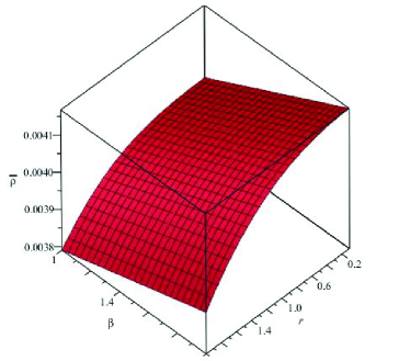
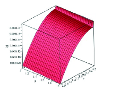
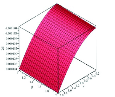
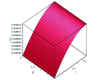
Figure 1: Plots of $\bar{\rho}$ (left plot, row-1), $\bar{P}_{r}$ (right plot, row-1), $\bar{P}_{t}$ (left plot, row-2) and $\bar{\Delta}$ (right plot, row-2) against $r$ using $M_{0}=1M_{\odot}$ and $R=(0.2)^{-1}M_{\odot}$ for solution-I.

The radial ($\bar{P}_{r}$) and tangential pressures ($\bar{P}_{t}$) show the same pattern against radius of stellar object while tangential pressure decreases with increase in $\beta$ as compared to radial (remains the same). It is seen that the radial pressure decreases when $\alpha$ increases as compared to the inverse behavior of tangential pressure for $\alpha$. The anisotropy parameter $\bar{\Delta}$ gives necessary information about anisotropy of the fluid configuration. For $\bar{P}_{t}>\bar{P}_{r}$, the anisotropy parameter remains positive which shows that it is outward directed while for $\bar{P}_{t}<\bar{P}_{r}$, it corresponds to inward directed. In our case, we measure anisotropy outward directed scenario (Figure 1, right plot, row-2). Moreover, the generic anisotropy remains the same for $\beta$ while increases with increase in $\alpha$. It is crucial to check the viability of the resulting solutions. For this purpose, we investigate the energy conditions which describe physically realistic matter configuration. The corresponding energy conditions are defined as

$$\bar{\rho}\geq 0,\quad\bar{\rho}+\bar{P}_{r}\geq 0,\quad\bar{\rho}+\bar{P}_{t}\geq 0,\quad\bar{\rho}-\bar{P}_{r}\geq 0,$$

$$\bar{\rho}-\bar{P}_{t}\geq 0,\quad\bar{\rho}+\bar{P}_{r}+2\bar{P}_{t}\geq 0.$$

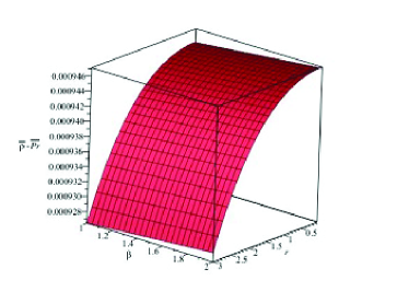
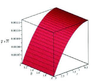
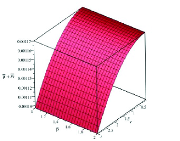
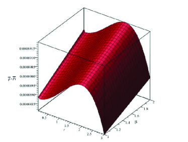
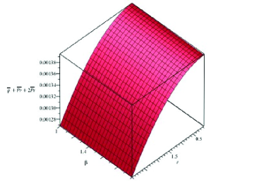
Figure 2: Plots of energy conditions against $r$ and $\beta$ using $M_{0}=1M_{\odot}$ and $R=(0.2)^{-1}M_{\odot}$ for solution-I.

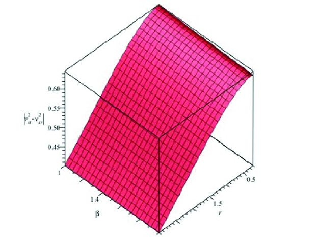
Figure 3: Plots of $|\nu_{st}^{2}-\nu_{sr}^{2}|$ against $r$ and $\beta$ using $M_{0}=1M_{\odot}$ and $R=(0.2)^{-1}M_{\odot}$ for solution-I.

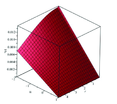
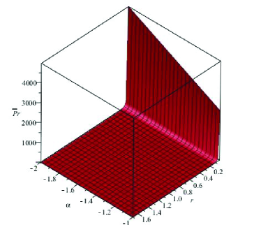
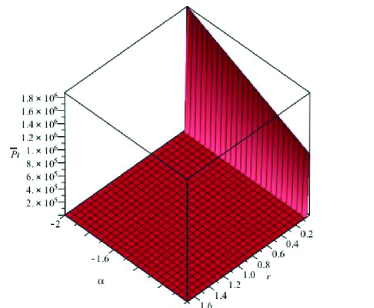
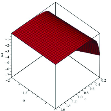
Figure 4: Plots of $\bar{\rho}$ (left plot, row-1), $\bar{P}_{r}$ (right plot, row-1), $\bar{P}_{t}$ (left plot, row-2) and $\bar{\Delta}$ (right plot, row-2) against $r$ and $\alpha$ using $M_{0}=1M_{\odot}$ and $R=(0.3)^{-1}M_{\odot}$ for solution-II.

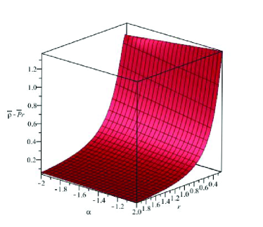
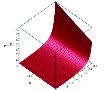
Figure 5: Plots of energy conditions against $r$ and $\alpha$ using $M_{0}=1M_{\odot}$ and $R=(0.3)^{-1}M_{\odot}$ for solution-II.

Figure 6: Plots of $|\nu_{st}^{2}-\nu_{sr}^{2}|$ against $r$ and $\alpha$ using $M_{0}=1M_{\odot}$ and $R=(0.3)^{-1}M_{\odot}$ for solution-II.

These conditions are shown graphically for the derived anisotropic solution in Figure 2 which indicates the validity of all energy condition and hence viability of the resulting anisotropic solution. For the stability analysis, we plot the squared speed of sound as shown in Figure 3. For stability of the solution, the condition $0<|\nu_{st}^{2}-\nu_{sr}^{2}|<1$, must be satisfied. Figure 3 shows $|\nu_{st}^{2}-\nu_{sr}^{2}|\leq 1$ for small $\alpha$ but it is violated for its large value.

For analyzing physical characteristics of solution-II, we choose constants $A$, $B$, $C$ from the matching conditions (36) and (50)-(51) whereas free parameters set as $c_{1}=-0.5$, $\beta=1.2$ and $n=3$, respectively. It is observed that the behavior of $\bar{\rho}$, $\bar{P}_{r}$ and $\bar{P}_{t}$ against $r$ is consistent with solution-I whereas both the radial and tangential pressure decreases linearly with increase in parameter $\alpha$ (Figure 4). The plot of these matter contents shows that as $r\rightarrow 0$, they attain their maximum and this, in fact, indicates the high compactness of the core of the star validating that our model under analysis is viable for the outer region of the core. Moreover, anisotropy is greater at the surface of star than that of core which shows opposite behavior as compared to solution-I. The plots of energy conditions (Figure 5) show that our solution satisfies all energy bounds which suffices for the viable solution. However, the stability condition is violated (Figure 6).

5 Concluding Remarks

Recently, the minimal gravitational decoupling approach has extensively been used to obtain exact solutions for interior configuration of stellar distribution. In this work, we have used MGD decoupling technique in $f(\mathcal{G})$ gravity to extend interior isotropic spherical solution to anisotropic solution contained in gravitational source. For this purpose, we have introduced a new source in isotropic energy-momentum tensor constituting the field equations for anisotropic matter distribution. We have introduced minimal geometrical deformation in metric functions (radial metric component only). It is found that the corresponding field equations with source can be split into two systems: one corresponds to standard field equations of $f(\mathcal{G})$ gravity and other contains the source term with deformed coefficients. These two systems express that there is a purely gravitational interaction, without direct exchange of energies.

We have studied junction condition for smooth matching of interior and exterior geometries for the deformed Schwarzschild spacetime. For anisotropic solution, we have taken a known solution then extended it through the source added in perfect fluid geometry. We have imposed constraints on the effective energy density and effective pressure which constitute solutions I and II, respectively. For physical acceptability, we have introduced specific generic function and examined energy conditions as well as squared speed of sound and anisotropy parameter. We have observed that solution-I as well as solution-II are physically acceptable and corresponds to stability of stellar object. Finally, we would like to mention here that our results for the first solution are consistent with those obtained in general relativity (GR) [14, 15]. It is also worth mentioning here that modified $f(\mathcal{G})$ gravity provides viable spherically symmetric solutions (as the energy conditions for both solutions are satisfied) due to inclusion of correction terms as compared to GR in which the second type of solutions do not meet the energy bounds [14, 15].

Appendix A

The GB corrections for the interior metric are

$$\kappa T_{0}^{0(\mathcal{G})} = \frac{1}{2}f(\mathcal{G})+\frac{e^{-2\psi}}{2r^{3}}[\eta^{\prime 2}(2r(9-\eta^{\prime}\psi^{\prime}r^{2}+4r\psi^{\prime}-6r\psi^{\prime})+r^{3}(\eta^{\prime 2}+\psi^{\prime 2})$$

$$+ 4\eta^{\prime}(4-r\psi^{\prime}+r^{2}\psi^{\prime 2}))+\exp(\psi)(\eta^{\prime}(-16+2r\psi^{\prime}-2r\eta^{\prime})-4r\eta^{\prime\prime})$$

$$+ 4r\eta^{\prime\prime}(1-r^{2}\eta^{\prime}\psi^{\prime}+r^{2}(1+\eta^{\prime 2})+4r\eta^{\prime}-2r\psi^{\prime})]\frac{df(\mathcal{G})}{d\mathcal{G}}-[\mathcal{G}^{\prime}(-8$$

$$+ r^{3}\psi^{\prime}\eta^{\prime 2}-r^{3}\psi^{\prime}\eta^{\prime}-2e^{\psi}r\psi^{\prime}+4r^{2}\psi^{\prime}\eta^{\prime}+2r^{3}\psi^{\prime}\eta^{\prime\prime}-4r^{2}\psi^{\prime 2}+6r\psi^{\prime}$$

$$+ 8e^{\psi})+\mathcal{G}^{\prime\prime}(4r(e^{\psi}-1)+8r^{2}(\psi^{\prime}-\eta^{\prime})+3r^{3}(\eta^{\prime}\psi^{\prime}-\eta^{\prime 2}-2\eta^{\prime\prime}))]\frac{e^{-2\psi}}{r^{3}}$$

$$\times \frac{d^{2}f(\mathcal{G})}{d\mathcal{G}^{2}}+\frac{2e^{-2\psi}}{r^{2}}[r^{2}(2\eta^{\prime\prime}-\eta^{\prime 2}-\eta^{\prime}\psi^{\prime})+4r(\eta^{\prime}-\psi^{\prime})$$

$$- 2e^{-\psi}(1-e^{-\psi})]\mathcal{G}^{\prime 2}\frac{d^{3}f(\mathcal{G})}{d\mathcal{G}^{3}},$$

$$\kappa T_{1}^{1(\mathcal{G})} = \frac{1}{2}f(\mathcal{G})+\frac{e^{-2\psi}}{2r^{3}}[4r\eta^{\prime 2}(1-e^{\psi}+r^{2}\eta^{\prime\prime}-4r\psi^{\prime})+4r^{2}\eta^{\prime}\eta^{\prime\prime}(r(\eta^{\prime}-\psi^{\prime})$$

$$+ 2)+\eta^{\prime 2}(2r(1+2r\eta^{\prime}-e^{\psi}-r^{2}\eta^{\prime}\psi^{\prime}-6r\psi^{\prime\prime})+r^{3}(\eta^{\prime}-\psi^{\prime}))$$

$$+ 2r\eta^{\prime}\psi^{\prime}(-7+e^{\psi}+4r\psi^{\prime})-16\psi^{\prime}(1-\psi^{\prime}-e^{\psi})]\frac{df(\mathcal{G})}{d\mathcal{G}}$$

$$+ \frac{e^{-2\psi}}{2r^{3}}[2r^{2}\eta^{\prime\prime}(-8-\eta^{\prime}r+e^{\eta-\psi}r\eta^{\prime}-2r\psi^{\prime})+\eta^{\prime}(4r(-7+e^{\psi}$$

$$+ 3r\psi^{\prime}-e^{\eta-\psi}r\psi^{\prime})-r^{3}\psi^{\prime 2})]\mathcal{G}^{\prime}\frac{d^{2}f(\mathcal{G})}{d\mathcal{G}^{2}}-\frac{e^{-2\psi}}{r^{2}}[r^{2}(2\eta^{\prime\prime}+\eta^{\prime 2}-\eta^{\prime}\psi^{\prime})$$

$$+ 4r(\eta^{\prime}-\psi^{\prime}-e^{\psi})+4]\mathcal{G}^{\prime 2}\frac{d^{3}f(\mathcal{G})}{d\mathcal{G}^{3}},$$

$$\kappa T_{2}^{2(\mathcal{G})} = \frac{1}{2}f(\mathcal{G})+\frac{e^{-2\psi}}{r^{4}}[r^{2}\eta^{\prime 2}(5-e^{\psi}+r\eta^{\prime}-2r\psi^{\prime})+r\eta^{\prime}(12-7r\psi^{\prime}$$

$$+ re^{\psi}\psi^{\prime}-12e^{\psi}+r^{2}\psi^{\prime 2})+2r^{2}\eta^{\prime\prime}(1-e^{\psi}+r\eta^{\prime}-r\psi^{\prime})-12r\psi^{\prime}$$

$$- 16e^{\psi}+8e^{2\psi}+12re^{\psi}\psi^{\prime}+4r^{2}\psi^{\prime 2}+8]\frac{df(\mathcal{G})}{d\mathcal{G}}+\frac{e^{-2\psi}}{2r^{3}}[4r^{2}\eta^{\prime\prime}\mathcal{G}^{\prime\prime}$$

$$+ \mathcal{G}^{\prime}(\eta^{\prime}(4r^{2}-r^{3}\psi^{\prime 2}-8r^{2}\psi^{\prime}+12r)+\eta^{\prime 2}r^{2}(r\psi^{\prime}+6)+2r^{2}\eta^{\prime\prime}(r\psi^{\prime}-6)$$

$$- 8(e^{\psi}-1)-2r\psi^{\prime}(r\psi^{\prime}+6))]\frac{d^{2}f(\mathcal{G})}{d\mathcal{G}^{2}}-2\frac{e^{-2\psi}}{r^{2}}\eta^{\prime}r\mathcal{G}^{\prime 2}\frac{d^{3}f(\mathcal{G})}{d\mathcal{G}^{3}}.$$

References

- [1] Nojiri, S. and Odintsov, S.D.: Phys. Lett. B 631(2005)1.
- [2] Calcagni, G., Tsujikawa, S. and Sami, M.: Class. Quantum. Grav. 22(2005)3977; De Felice, A., Hindmarsh, M. and Trodden, M.: J. Cosmol. Astopart. Phys. 08(2006)005.
- [3] Bamba, K. et al.: Eur. Phys. J. C 67(2010)295.
- [4] Mak, M.K., Harko, T.: Int. J. Mod. Phys. D 13(2004)149.
- [5] Gleiser, M. and Dev, K.: Int. J. Mod. Phys. D 13(2004)1389.
- [6] Sharma, R. and Maharaj, S.D.: Mon. Not. R. Astron. Soc. 375(2007)1265.
- [7] Kalam, M., Rahaman, F., Hossein, S.M. and Ray, S.: Eur. Phys. J. C 73(2013)2409.
- [8] Bhar, P., Rahaman, F., Ray, S. and Chatterjee, V.: Eur. Phys. J. C 75(2015)190.
- [9] Maurya, S.K., Gupta, Y.K. and Ray, S.: Eur. Phys. J. C 77(2017)360.
- [10] Ovalle, J.: Mod. Phys. Lett. A 23(2008)3247.
- [11] Ovalle, J. and Linares, F.: Phys. Rev. D 88(2013)104026.
- [12] Casadio, R., Ovalle, J. and da Rocha, R.: Class. Quantum Grav. 32(2015)215020.
- [13] Ovalle, J.: Phys. Rev. D 95(2017)104019.
- [14] Ovalle, J., Casadio, R., da Rocha, R. and Sotomayor, A.: Eur. Phys. J. C 78(2018)122.
- [15] Sharif, M. and Sadiq, S.: Eur. Phys. J. C 78(2018)410.
- [16] Zubair, M. and Abbas, G.: arXiv:1412.2120.
- [17] Abbas, G., Kanwal, A. and Zubair, M.: Astrophys. Space Sci. 357(2015)109.
- [18] Abbas, G. et al.: Astrophys. Space Sci. 357(2015)158.
- [19] Sharif, M. and Fatima, I.: Int. J. Mod. Phys. D 25(2016)1650083.
- [20] Sharif, M. and Naz, S.: Mod. Phys. Lett. A 33(2018)1850109.
- [21] Burikham, P., Harko, T. and Lake, M.J.: Phys. Rev. D 94(2016)064070.
- [22] Krori, K.D. and Barua, J.: J. Phys. A: Math. Gen. 8(1975)508.
- [23] Harko, T. and Mak, M.K.: Ann. Phys. 11(2002)3; ibid. Proc. Roy. Soc. Lond. A 459(2003)393; Harko, T., Dobson, P.N.Jr. and Mak, M.K. : Int. J. Mod. Phys. D 11(2002)207; Graterol, R.P. : Eur. Phys. J. P 133(2018)244.
- [24] Cognola, G. et al.: Phys. Rev. D 73(2006)084007.