A general framework for quantum splines

Abstract.

Quantum splines are curves in a Hilbert space or, equivalently, in the corresponding Hilbert projective space, which generalize the notion of Riemannian cubic splines to the quantum domain. In this paper, we present a generalization of this concept to general density matrices with a Hamiltonian approach and using a geometrical formulation of quantum mechanics. Our main goal is to formulate an optimal control problem for a nonlinear system on $\mathfrak{u}^{*}(n)$ which corresponds to the variational problem of quantum splines. The corresponding Hamiltonian equations and interpolation conditions are derived. The results are illustrated with some examples and the corresponding quantum splines are computed with the implementation of a suitable iterative algorithm.

1. Introduction

Quantum control theory, and in particular quantum optimal control, is drawing considerable attention from quite different communities in different areas of physics, chemistry, applied mathematics and quantum information (see [23] for a nice introduction to the area with several practical physical and chemical applications). This subject represents an essential ingredient to use the new quantum technologies which are being created in these fields, with a wide range of applications (see, for instance, [5, 6, 16, 18, 22, 24, 25, 26]). An important problem is the design of efficient algorithms to generate accurately specified quantum states under certain conditions (in minimal time, with a minimal energy investment, etc). These algorithms usually consist in defining a suitable time dependent Hamiltonian which drives the system to the desired quantum states under the required conditions.

In a recent paper [9], Brody and co-workers introduced the notion of quantum spline as the generalization to the quantum domain of the familiar notion of geometric splines (see [12, 13, 15, 21]). A quantum spline is the solution of the following quantum optimization problem. Let us consider a set of states $\{|\psi_{0}\rangle,\cdots,|\psi_{N}\rangle\}$ in a certain finite dimensional Hilbert space ${\mathcal{H}}$ and a corresponding set of times $\{t_{0},\cdots,t_{N}\}$. The problem is to find a time-dependent Hamiltonian $H(t)$ defining an unitary evolution which, at the given times $t_{k}$, passes arbitrarily close to the given states $|\psi_{k}\rangle$, and such that the total change in the Hamiltonian along the curve is minimized. We can write it as a variational problem asking to minimize the cost functional

$${\mathcal{J}}=\int_{t_{0}}^{t_{N}}\langle\mathrm{i}\dot{H}(t)\mid\mathrm{i}\dot{H}(t)\rangle\mathrm{d}t+\frac{1}{2\epsilon}\sum_{k=1}^{N}D^{2}(|\psi(t_{k})\rangle,|\psi_{k}\rangle)$$ (1)

where $|\psi(t)\rangle=U(t)|\psi_{0}\rangle$ represents the trajectory in ${\mathcal{H}}$ defined by the unitary evolution $U(t)$, the scalar product $\langle\cdot\mid\cdot\rangle$ represents the trace of the product

$$\langle A\mid B\rangle=-\frac{1}{2}\mathrm{Tr}(AB),\qquad\forall A,B\in\mathfrak{u}(\mathcal{H}),$$ (2)

and $\epsilon$ is just a positive coefficient which allows us to change the relative importance of the total change of the Hamiltonian of the system and how close we are from the point we are supposed to target ($D$ represents the corresponding distance).

Some comments are in order:

• As the time dependence of the Hamiltonian in quantum control problems is often implemented as time-dependent magnetic fields which interact with the spin system, we can think at the minimization problem as the equilibrium between the accuracy at targetting the points at the designated times and the total energy required to change the magnetic fields during the process.

• The (square) distances $D^{2}(|\psi(t_{k})\rangle,|\psi_{k}\rangle)$ are considered on the projective space ${\mathcal{P}H}$, with respect to the canonical Fubini-Study metric. From the technical point of view, the functional (1) combines thus quantities defined on two different manifolds: the trace-norm of skew-Hermitian operators and the Fubini-Study metric on the projective space.

• The solution of the problem above, even for very simple examples such as a two-level quantum system, requires of numerical algorithms. In [9] the authors provide an algorithm for the discretization of their variational equations which is used in the construction of the solution of the example they study.

The aim of this paper is to introduce an alternative formulation of the problem of quantum splines and a generalization of the notion which enlarges the range of potential applications. The main idea is to re-formulate the problem in terms of density matrices and to adapt the conditions on the dynamics to it. Thus, the notion of quantum spline for pure states introduced in [9] is included, while an analogous notion for mixed states does also make sense:

New formulation of the interpolation problem: Let us consider a set of density matrices $\{\rho_{0},\cdots,\rho_{N}\}$ on a certain finite dimensional Hilbert space ${\mathcal{H}}$ and a corresponding set of times $\{t_{0},\cdots,t_{N}\}$. Find a time-dependent Hamiltonian $H(t)$ defining an unitary evolution which, at the given times $t_{k}$, passes as close as possible to the given points $\rho_{k}$, and such that the change in the Hamiltonian is optimal in the sense that the cost functional $${\mathcal{J}}=\sum_{{k=1}}^{N}\int_{t_{k-1}}^{t_{k}}\langle\mathrm{i}\dot{H}(t)\mid\mathrm{i}\dot{H}(t)\rangle\mathrm{d}t+\frac{1}{2\epsilon}\sum_{k=1}^{N}d^{2}(\rho(t_{k}),\rho_{k})$$ (3) is minimized, where the trajectory of the system represented by $\rho(t)$ is a solution of von Neumann equation: $$\mathrm{i}\hbar\dot{\rho}(t)=H(t)\rho(t)-\rho(t)H(t),$$ (4) and $d$ represents the distance on the space of Hermitian operators $d(A,B)=\sqrt{\frac{1}{2}\mathrm{Tr}(A-B)^{2}}$.

This formulation of the problem includes the previous one for the case of pure quantum states, but it allows to consider it also for general quantum states. Furthermore, it relaxes the continuity condition on the derivative of the Hamiltonian $H(t)$ at the intermediate points, as it is often assumed in (quantum) control based on pulses. From a physical point of view, the lack of continuity does not represent a serious condition on the system, and as we are going to see it allows for a much simpler analysis of the problem.

Regarding the generalization to density matrices, notice that all real systems are in contact with some type of environment. In that case, we know that the system is very seldom in a pure quantum state and therefore to extend the notion of quantum spline to mixed states seems as a natural step forward. For instance, we could consider a system which initially is in equilibrium at a finite temperature $T$ (see [7]) with a bath. If the evolution associated to the quantum controls is much faster than the dynamics produced by the interaction with the bath, we could approximate the evolution by a unitary transformation on the set of mixed quantum states. This is the type of problem that we will be considering in this paper. Another interesting generalization would be to consider that the controlled evolution is of the same order as the interaction with the bath and replace von Neumann equation by a more general master equation, such as Lindblad-Kossakowski equation. The problem would be formally analogous to our “New formulation” above, replacing equation (4) by Lindblad-Kossakowski equation. Nonetheless, Lindblad-Kossakowski equation would put some constraints in the possible values of the set of times $\{t_{j}\}$ and density matrices $\{\rho_{j}\}$ (remember that Lindblad dynamics is not always controllable [2, 3]). We are also studying this problem and it will be considered in a future paper.

There are important aspects that characterize the new formulation:

• From the technical point of view, our formulation is much simpler than the one considered in [9], since it can be done at the level of a linear space (the dual space to the algebra of the unitary group $\mathfrak{u}^{*}(n)$), instead of considering the Lie group $U(n)$ and the projective space $\mathbb{CP}^{n-1}$.

• The set of quantum states $\mathcal{D}$ for our formulation will be the submanifold of $\mathfrak{u}^{*}(n)$ defined by the elements which have trace equal to one and are positive definite. $\mathcal{D}$ is a nonlinear submanifold of $\mathfrak{u}^{*}(n)$, but the particular choice of our dynamic system allows us to treat the problem as a problem defined on the linear space $\mathfrak{u}^{*}(n)$. Indeed, as the dynamics on $\mathcal{D}$ is defined by von Neumann equation, we know that the solution $\rho(t)$ must belong to a unitary orbit of the coadjoint action of the unitary group. As it is well known (see [20]), those orbits constitute symplectic submanifolds of $\mathfrak{u}^{*}(n)$ which define the leaves of the symplectic foliation associated with its Lie-Poisson canonical structure. If we consider an initial condition contained in one of the leaves, the whole solution will be contained in it. This property will allow us to consider the problem defined directly at the linear space $\mathfrak{u}^{*}(n)$ and forget about the nonlinear constraints. Nonetheless, this also imposes some constraints for the definition of splines in the general case. Indeed, as the dynamics we are considering is always unitary, any generalized spline will be contained in a unitary orbit. Thus, if the target points are not contained in one unitary orbit, the best possible solution will only be able to define the closest unitary orbit to the set of target points. We will discuss this point at the end of the paper.

• The geometric formulation of Quantum Mechanics (see [4, 8, 10, 19] ) is a natural framework to formulate the problem in a geometric formalism which exhibits these symplectic aspects. In that framework, von Neumann equation defines in a natural way a Hamiltonian vector field. This property is particularly useful when considering numeric integration of the solutions, since by using symplectic integrators we do not need to take into account constraints such as the trace of the quantum state or its rank and the problem can be treated as a free one.

• In [9], a numerical algorithm was introduced in order to provide a method of integration for the splines. In our formalism, even if simpler, a numerical algorithm will also be necessary. We introduce an iterative algorithm to approach the optimal solution of the interpolation problem. We may not reach the absolute optimal solution, but we always obtain a very good approximation to it. As our framework is defined on linear spaces the algorithm turns out to be very simple and the efficiency is very high.

The structure of the paper is as follows. Section 2 presents a summary of the geometric formalism of quantum mechanics, with special emphasis on the geometrical structures associated with the description of the set of Hermitian operators and the set of density states, which are the main ingredients of our construction. Section 3 presents the main aspects of our new formulation, analyzing first the quantum control problem from the point of view of the Pontryagin maximum principle, then the analytical tools used to build the system of differential equations defining the solution and finally discussing an iterative algorithm to build solutions in an efficient way and the numerical methods we use to obtain them. Section 4 illustrates our construction with the simplest example for the interpolation between a set of pure states of a two level system and Section 5 presents a more sophisticated example of the interpolation of mixed states of a three level quantum systems. Finally, Section 6 summarizes the main results of the paper and discuss the possible generalization of our method to the case of open quantum systems.

2. The geometrical description of quantum mechanics

Let us briefly review some very general aspects of the geometrical formulation of quantum mechanics, focusing on the ingredients which will be used later in the paper. For more details, we address the interested reader to [4, 8, 10, 19] and references therein. We use Einstein summation over repeated indexes.

2.1. The geometrical structures of $\mathfrak{u}^{*}(n)$

We hereafter assume $\mathcal{H}$ to be an $n$-dimensional complex Hilbert space. In this case the $C^{*}$–algebra of operators corresponds to $\mathcal{A}=\mathrm{End}(\mathbb{C}^{n})$ and the involution is the usual adjoint operation for complex endomorphisms. In this case, when considering an orthonormal basis, self-adjoint operators are represented by Hermitian matrices.

It is important now to emphasize the following facts:

• We can define isomorphisms between $\mathfrak{u}(n)$, $\mathfrak{u}^{*}(n)$ and the vector space of Hermitian matrices $\mathrm{i}\mathfrak{u}(n)$ by mappings

  $$\mathrm{i}\mathfrak{u}(n)\ni A\mapsto iA\,\in\mathfrak{u}(n);$$ (5)

  $$\mathrm{i}\mathfrak{u}(n)\ni A\mapsto\xi_{A}\,\in\mathfrak{u}^{*}(n),\;\;\;\mbox{with}\;\;\xi_{A}=\langle-\mathrm{i}A\mid\cdot\,\rangle:\mathfrak{u}(n)\to\mathbb{R}.$$ (6)

  These isomorphisms define also Lie brackets on each space $[\cdot,\cdot]_{\mathfrak{u}}$, $[\cdot,\cdot]_{\mathfrak{u}^{*}}$ and $[\cdot,\cdot]_{\mathrm{i}\mathfrak{u}}$. We have a special interest in the identification of the elements of $\mathfrak{u}^{*}(n)$ with the Hermitian matrices, which will be used later.

• On the dual space $\mathfrak{u}^{*}(n)$ we have a natural linear Poisson structure, the Lie-Poisson structure. The Poisson tensor $\Lambda$ is defined, on the set of linear functions on $\mathfrak{u}^{*}(n)$, as follows

  $$\Lambda_{\xi}(V,W)=\xi\left([V,W]\right),\qquad\xi\in\mathfrak{u}^{*}(n),\quad\forall V,W\in\mathfrak{u}(n).$$ (7)

  From this definition on linear functions, we can construct the Poisson bracket on general functions $f,g\in{\mathcal{C}}^{\infty}(\mathfrak{u}^{*}(n))$ by extending equation (7) requiring bilinearity, i.e., as the action of the bi-differential operator which on linear functions behaves as equation (7). This defines the canonical Lie-Poisson tensor of the dual of the unitary algebra (see [1]).

• The Hamiltonian vector field $X_{\mathrm{i}H}=-\Lambda(\mathrm{i}H,\cdot)$ is the infinitesimal generator of the coadjoint action of $U(n)$ on $\mathfrak{u}^{*}(n)$ and, therefore, the system

  $$\dot{\xi}(t)=X_{\mathrm{i}H}(\xi(t)),\qquad\xi(0)=\xi_{0},\qquad\xi(t)\in\mathfrak{u}^{*}(n),$$ (8)

  is a symplectic Hamiltonian system on the coadjoint orbit where the initial condition $\xi_{0}$ is contained (again we refer the reader to [1] for details) .

2.2. The set of density matrices ${\mathcal{D}}({\mathcal{H}})$

The physical states which are used in the Schrödinger formalism correspond to the points of the projective space ${\mathcal{P}H}$. As it is well known, we can also represent these states by using the projectors on one-dimensional subspaces of the Hilbert space. Unitary evolution, associated with the Schrödinger or the von Neumann equation, will define trajectories on this set. We will denote by ${\mathcal{D}}^{1}({\mathcal{H}})$ the corresponding set of projectors. Nonetheless, ${\mathcal{D}}^{1}({\mathcal{H}})$ is not enough to represent all the possible physical states of a system, since arbitrary convex combinations of rank-one-projectors also define admissible physical states. Indeed, if our system is not isolated and is surrounded by an environment (as it is the case of all real systems), or just a set of other systems, the representing state will not be, in general, pure. Therefore, we must enlarge the set of states to consider:

Definition 2.1.

The set of density states ${\mathcal{D}}({\mathcal{H}})$ of the system corresponds to the subset of $\mathfrak{u}^{*}(n)$ obtained by convex combinations of rank-one-projectors, that is,

$${\mathcal{D}}({\mathcal{H}})=\left\{\rho=\sum_{k}p_{k}\rho_{k}\;:\quad p_{k}\geq 0,\quad\sum_{k}p_{k}=1,\quad\rho_{k}\in{\mathcal{D}}^{1}({\mathcal{H}})\right\}.$$ (9)

Equivalently, we can consider the following definition: an element $\rho\in\mathfrak{u}^{*}(n)$ is a density operator if and only if

$$\mathrm{Tr}\rho=1\quad\mbox{and}\quad\rho\geq 0.$$ (10)

An important property of the manifold $\mathcal{D}(\mathcal{H})$ is its internal structure, in particular in what regards the restriction of the coadjoint orbits of the unitary group on $\mathfrak{u}^{*}(n)$. A very important aspect of that structure is the nature of $\mathcal{D}(\mathcal{H})$ as a stratified manifold, the strata being defined by the rank of the states (see [Grabowski2005a] for details). Indeed, as all density states are self-adjoint and positive definite, they all are diagonalizable and have non-negative eigenvalues. The number of non-vanishing eigenvalues equals the rank of the operator (or the matrix, if we choose a basis). Thus, all states having the same rank belong to the same stratum. As the coadjoint action of the unitary group is known to preserve the spectrum of the density operator, it is obvious that the orbit will stay on the same stratum as its initial condition. Equivalently, we can claim that the Hamiltonian vector field defined by equation (8) will be tangent to the different strata.

Thus, if we consider the Hamiltonian vector field $X_{\mathrm{i}H}$ (defined by equation (8)) restricted to $\mathcal{D}(\mathcal{H})$, we obtain the von Neumann equation for the density matrix $\rho\in\mathcal{D}(\mathcal{H})$,

$$\dot{\rho}=X_{\mathrm{i}H}(\rho).$$ (11)

We know that this evolution corresponds to a unitary transformation. Thus, the Hamiltonian vector fields of $\Lambda$ are the infinitesimal generators of the coadjoint action of the unitary group on $\mathfrak{u}^{*}(n)$, and the corresponding orbits are known to be symplectic submanifolds. For instance, the set of pure states $\mathcal{D}^{1}(\mathcal{H})$ defines a symplectic orbit which corresponds to a symplectic leaf of the canonical Poisson foliation. Therefore, the solution of von Neumann’s equation on $\mathcal{D}^{1}(\mathcal{H})$ is always tangent to it and defines a symplectic transformation. This allows us to use the formulation of the problem on $\mathfrak{u}^{*}(n)$ without using any constraints to specify the submanifold of pure states, since we know that any trajectory with an initial condition on $\mathcal{D}^{1}(\mathcal{H})$ will remain on the submanifold for all times.

For the case of a mixed state, the situation is analogous, but in this case the symplectic orbit of the coadjoint action will not cover all the stratum. Each stratum will contain several coadjoint orbits of different dimensions and therefore the formulation of the interpolation problem must take into account this property. Indeed, the exact quantum spline for mixed states (i.e., a curve joining all points) makes sense only if the set of points belong to the same coadjoint orbit. As the target points are not reached exactly, the problem still makes sense for a neighborhood of the orbit. In the next Section we will see how it is possible to define an iterative algorithm which drives the evolution to the closest point of the orbit with respect to the target point.

3. Dynamical interpolation problem on $\mathfrak{u}^{*}(n)$

Let $\{\rho_{0},\rho_{1},\cdots,\rho_{N}\}$ be a finite subset of $\mathcal{D}(\mathcal{H})$ and $0=t_{0}<t_{1}<\cdots<t_{N}=T$ a partition of the time interval $[0,T]$, $T>0$. Consider also a $m$-dimensional vector subspace $\mathfrak{h}$ of $\mathfrak{u}^{*}(n)$, $m\leq n^{2}$ which will represent the space of admissible controls for our interpolation problem.

3.1. The control problems chain

In general, let $E$ be a real vector space of dimension $n$ and $U$ a subspace of $E$ (in our case, $E$ will be the vector space $\mathfrak{u}^{*}(n)\times\mathfrak{u}^{*}(n)$). Given a cost function $L:E\times U\to\mathbb{R}$ and the functions $G_{j}:E\to\mathbb{R}$, consider the optimal control problem P concerning the minimum of the functional

$$J(u)=\sum_{j=1}^{N}\int_{t_{j-1}}^{t_{j}}L(x(t),u(t))\,\mathrm{d}t+\frac{1}{\epsilon}\sum_{j=1}^{N}G_{j}(x(t_{j})),$$ (12)

where $\epsilon$ is a tunable positive parameter, and with $u:[0,T]\to U$ and $x:[0,T]\to E$ being curves, subject to the initial condition $x(0)=x_{0},$ satisfying the control system

$$\dot{x}=f(x,u)$$ (13)

and the conditions:

• $x$ is continuous in $[0,T]$ and smooth in $]t_{j-1},t_{j}[$, with finite one-sided limits at $t_{j}$, for all $j=1,\ldots,N$;

• $u$ is smooth in $]t_{j-1},t_{j}[$, with finite one-sided limits at $t_{j}$, for all $j=1,\ldots,N$.

This defines a set of $N$ subproblems $P_{j}$, $j=1,\ldots,N$, one for each subinterval, where the initial condition is fixed (by the value of the solution at the end point of the previous interval), but the final condition is free. Thus, on interval $]t_{j-1},t_{j}[$ we consider the functional

$$J_{j}(u)=\int_{t_{j-1}}^{t_{j}}L(x(t),u(t))\,\mathrm{d}t+\frac{1}{\epsilon}G_{j}(x(t_{j}),$$ (14)

and search for the optimal solution $x:[t_{j-1},t_{j}]\to\mathbb{R}$ subject to the initial conditions $x(t_{j-1})=x_{j-1}$, which corresponds to the final conditions of the previous subinterval. Each of these subproblems is a particular case of a well known optimal control problem known as a Bolza problem (see [11]). The solution $x(t)$ is asked to be continuous on the whole interval $[0,T]$.

The solution of each Bolza problem can be obtained straightforwardly by using the Pontryagin maximum principle, the only difficulty being the boundary condition. Although it is a well known method, let us present, for completeness, a sketch of the variational construction needed to prove Pontryagin’s result. Let us take, for instance, the first subinterval $[t_{0},t_{1}]$. Consider the Hamiltonian function $h:E\times E^{*}\times U\to\mathbb{R}$ associated with the optimal control problem, defined by

$$h(x,p,u)=p(f(x,u))-L(x,u).$$ (15)

For each $x\in E$ and $p\in E^{*}$, the partial functional derivative of a function $h$ with respect to $x$ at $a$ is an element of $E^{*}$ denoted by $(\delta h/\delta x)(a)$ and the partial functional derivative with respect to $p$ at $a$ is an element of $E$ denoted by $(\delta h/\delta p)(a)$. Now, let us enlarge the functional $J$ by the dynamical constraints, using the costate trajectory $p:[t_{0},t_{1}]\to E$, in the following way:

$$\widetilde{J}(u) = \displaystyle\int_{t_{0}}^{t_{1}}L(x(t),u(t))\,\mathrm{d}t+\int_{t_{0}}^{t_{1}}p\left(\dot{x}-f(x,u)\right)\,\mathrm{d}t+\frac{1}{\epsilon}G_{1}(x(t_{1}))$$

$$= \displaystyle\int_{t_{0}}^{t_{1}}\left(L(x,u)-p(f(x,u))\right)\mathrm{d}t+\int_{t_{0}}^{t_{1}}p(\dot{x})\,\mathrm{d}t+\frac{1}{\epsilon}G_{1}(x(t_{1}))$$

$$= \displaystyle-\int_{t_{0}}^{t_{1}}h(x,p,u)\mathrm{d}t+\int_{t_{0}}^{t_{1}}p(\dot{x})\,\mathrm{d}t+\frac{1}{\epsilon}G_{1}(x(t_{1})).$$

Thus, we know that the optimal solution will satisfy the equations

$$\dot{x}=\frac{\delta h}{\delta p},\qquad\dot{p}=\displaystyle-\frac{\delta h}{\delta x},\qquad p(t_{1}^{-})=-\frac{1}{\epsilon}\frac{\delta G_{1}}{\delta x}(x(t_{1})),\qquad\frac{\delta h}{\delta u}(x,p,u)=0.$$ (16)

Therefore, it is now simple to prove the following result:

Theorem 1.

If $u$ is the optimal control resulting of the optimal control problems $P_{j}$, $j=1,\ldots,N$ and $x$ is the associated optimal state trajectory, then there exists a piecewise-smooth costate trajectory $p:[0,T]:\rightarrow E$ such that

$$\displaystyle\dot{x}=\frac{\delta h}{\delta p},\qquad\dot{p}=-\frac{\delta h}{\delta x},$$ (17)

$$\frac{\delta h}{\delta u}=0,$$ (18)

$$\displaystyle p(t_{j}^{-})=-\frac{1}{\epsilon}\frac{\delta G_{j}}{\delta x}(x(t_{j})),\qquad\mbox{for all}\quad j=1,\ldots,N.$$ (19)

Proof

The problem is defined piecewisely, and hence we will proceed in the same way. For each $j$, consider the problem on the subinterval $[t_{j-1},t_{j}]$, determine the optimal solution on it, and consider then the value of the optimal solution to define the boundary condition of the next subinterval in order to ensure continuity of the trajectory. On the first subinterval, $[t_{0},t_{1}]$, we have seen that the solution satisfies the condition. Consider now the optimal solution $x(t)$ and the corresponding value $x(t_{1})$, and use it as the initial condition for the Bolza problem in the subinterval $[t_{1},t_{2}]$. We will then define an optimal solution for the second subinterval which will define the initial condition for the third one. On each case we produce a smooth costate variable $p$, defined on each subinterval. If we repeat the procedure on all subintervals, the result follows and the global costate variable will be, by construction, piecewise-smooth.  $\Box$

Observe that system (17-18) and the time-invariance of the Hamiltonian $h$ guarantee that $h$ is an integral of motion.

3.2. The optimal control problem P for quantum splines

Let us apply now the result above to our formulation of the interpolation problem. As we had formulated it on $\mathfrak{u}^{*}(n)$, we consider a cost function $L:\mathfrak{u}^{*}(n)\times\mathfrak{u}^{*}(n)\times\mathfrak{h}\to\mathbb{R}$ defined by

$$L(\rho,H,u)=\frac{1}{2}\left\|u\right\|^{2}=\frac{1}{2}\langle u,u\rangle$$ (20)

where $\langle\xi,\eta\rangle=\frac{1}{2}\mathrm{Tr}(\xi\eta)$ for $\xi,\eta\in\mathfrak{u}^{*}(n)$. The functions $G_{j}:\mathfrak{u}^{*}(n)\to\mathbb{R}$ are given by

$$G_{j}(\rho)=\frac{1}{2}\left\|\rho-\rho_{j}\right\|^{2},\qquad j=1,\ldots,N.$$ (21)

The dynamical interpolation problem is the optimal control problem concerning the minimum of the functional

$$J(u)=\sum_{j=1}^{N}\int_{t_{j-1}}^{t_{j}}L(\rho(t),H(t),u(t))\,\mathrm{d}t+\frac{1}{\epsilon}\sum_{j=1}^{N}G_{j}(\rho(t_{j})),$$ (22)

with $u:[0,T]\to\mathfrak{h}$ and $(\rho,H):[0,T]\to\mathfrak{u}^{*}(n)\times\mathfrak{u}^{*}(n)$ being piecewise-defined curves subject to the initial conditions

$$\rho(0)=\rho_{0}\qquad\mbox{and}\qquad H(0)=H_{0},$$ (23)

satisfying the control system

$$\dot{\rho}={\color[rgb]{0,0,0}[H,\rho]_{\mathfrak{u}^{*}}},\qquad\dot{H}=u,$$ (24)

where the curves verify the same regularity conditions of the previous section.

The Hamiltonian function to apply the Pontryagin maximum principle becomes now the function $h:\mathfrak{u}^{*}(n)\times\mathfrak{u}^{*}(n)\times\mathfrak{u}(n)\times\mathfrak{u}(n)\times\mathfrak{h}\to\mathbb{R}$ given by

$$h(\rho,H,\Gamma,\Pi,u)=\Gamma({\color[rgb]{0,0,0}[H,\rho]_{\mathfrak{u}^{*}}})+\Pi(u)-L(\rho,H,u).$$ (25)

The approach considered above, obtained by application of the theorem 1, implies the following result:

Theorem 2.

If $u$ is the optimal control resulting of the optimal control problems $P_{j}$, $j=1,\ldots,N$, and $(\rho,H)$ is the associated optimal state trajectory, then there exists a piecewise-continuous optimal costate trajectory $(\Gamma,\Pi)$ that satisfies the system

$$\dot{\rho}={\color[rgb]{0,0,0}[H,\rho]_{\mathfrak{u}^{*}}},\quad\dot{H}=u,\quad\dot{\Gamma}=-{\rm ad}_{H}^{*}\Gamma,\quad\dot{\Pi}=\,{\rm ad}_{\rho}^{*}\Gamma,\quad\Pi=u^{\flat},$$ (26)

the initial conditions (23) and the interpolating conditions

$$\Gamma(t_{j}^{-})=-\frac{1}{\epsilon}(\rho(t_{j})-\rho_{j})^{\flat},\qquad\Pi(t_{j}^{-})=0,\qquad\,j=1,\ldots,N.$$ (27)

In the equations above $\mathrm{ad}$ and $\mathrm{ad}^{*}$ refer to the adjoint and co-adjoint actions of the Lie bracket $[\cdot,\cdot]_{\mathfrak{u}^{*}}$ and ${\cdot}^{\flat}$ specifies the isomorphism $\flat:\mathfrak{u}^{*}\to\mathfrak{u}$ given by the inner product on $\mathfrak{u}^{*}(n)$.

Notice that eliminating the controls in (26) we obtain the system

$$\dot{\rho}={\color[rgb]{0,0,0}[H,\rho]_{\mathfrak{u}^{*}}},\qquad\dot{H}=\Pi_{\mathfrak{h}}^{\sharp},\qquad\dot{\Gamma}=-{\rm ad}_{H}^{*}\Gamma,\qquad\dot{\Pi}=\,{\rm ad}_{\rho}^{*}\Gamma,$$ (28)

which is Hamiltonian with respect to the function $\tilde{h}:\mathfrak{u}^{*}(n)\times\mathfrak{u}^{*}(n)\times\mathfrak{u}(n)\times\mathfrak{u}(n)\to\mathbb{R}$,

$$\tilde{h}(\rho,H,\Gamma,\Pi)=\Gamma({\color[rgb]{0,0,0}[H,\rho]_{\mathfrak{u}^{*}}})+\frac{1}{2}\left\|\Pi_{\mathfrak{h}}^{\sharp}\right\|^{2}.$$ (29)

Notice that ${\cdot}^{\sharp}$ specifies the inverse of the isomorphism $\flat$.

Observe that the Hamiltonian system (28) can be written as follows

$$\dot{\rho}={\color[rgb]{0,0,0}[H,\rho]_{\mathfrak{u}^{*}}},\qquad\dot{H}=\Pi_{\mathfrak{h}}^{\sharp},\qquad\dot{\Gamma}={\color[rgb]{0,0,0}[H,\Gamma^{\sharp}]_{\mathfrak{u}^{*}}^{\flat}},\qquad\dot{\Pi}={\color[rgb]{0,0,0}[\Gamma^{\sharp},\rho]_{\mathfrak{u}^{*}}^{\flat}},$$ (30)

with interpolation conditions

$$\Gamma(t_{j}^{-})=-\frac{1}{\epsilon}(\rho(t_{j})-\rho_{j})^{\flat},\qquad\Pi(t_{j}^{-})=0,\qquad j=1,\ldots,N.$$ (31)

Consider now the problem $P$ with $u$ taking values in all space, that is, the space of admissible controls corresponds to $\mathfrak{h}=\mathfrak{u}^{*}(n)$ and thus $m=n^{2}$. From Hamiltonian equations (30), we differentiate twice the equation $\dot{H}=\Pi^{\sharp}$ and eliminate the costates $\Gamma$ and $\Pi$, to obtain the equations $\ddot{H}=-\mathrm{ad}_{\rho}\Gamma^{\sharp}$ and $\dddot{H}={\color[rgb]{0,0,0}[H,\ddot{H}]_{\mathfrak{u}^{*}}}$. Indeed,

$$\begin{array}[]{lll}\displaystyle\dddot{H}&=&-\,{\rm ad}_{\dot{\rho}}\Gamma^{\sharp}-\,{\rm ad}_{\rho}\dot{\Gamma}^{\sharp}=-{\rm ad}_{[H,\rho]_{\mathfrak{u}^{*}}}\Gamma^{\sharp}-\,{\rm ad}_{\rho}{\rm ad}_{H}\Gamma^{\sharp}\\[5.0pt] &=&{\rm ad}_{\rho}{\rm ad}_{H}\Gamma^{\sharp}-{\rm ad}_{H}{\rm ad}_{\rho}\Gamma^{\sharp}-\,{\rm ad}_{\rho}{\rm ad}_{H}\Gamma^{\sharp}\\[5.0pt] &=&-{\rm ad}_{H}{\rm ad}_{\rho}\Gamma^{\sharp}={\rm ad}_{H}\ddot{H}={\color[rgb]{0,0,0}[H,\ddot{H}]_{\mathfrak{u}^{*}}}.\end{array}$$ (32)

Therefore, the associated optimal state trajectory $(\rho,H)$ verifies the two conditions

$$\dot{\rho}={\color[rgb]{0,0,0}[H,\rho]_{\mathfrak{u}^{*}}}\qquad\mbox{and}\qquad\displaystyle\dddot{H}={\color[rgb]{0,0,0}[H,\ddot{H}]_{\mathfrak{u}^{*}}}.$$ (33)

Moreover, interpolation conditions can be interpreted in terms of $\rho$ and $H$ as follows: $\rho$ is of class $\mathcal{C}^{1}$, $H$ is of class $\mathcal{C}^{0}$ and

$$\ddot{H}(t_{j}^{-})=\frac{1}{\epsilon}{\color[rgb]{0,0,0}[\rho_{j},\rho(t_{j})]_{\mathfrak{u}^{*}}},\qquad\dot{H}(t_{j}^{-})=0,\qquad\mbox{for all}\quad j=1,\ldots,N.$$ (34)

Now, if we integrate the equation $\displaystyle\dddot{H}=[H,\ddot{H}]_{\mathfrak{u}^{*}}$, we obtain

$$\ddot{H}(t)=K_{j}+{\color[rgb]{0,0,0}[H(t),\dot{H}(t)]_{\mathfrak{u}^{*}}},\qquad\mbox{with}\quad t\in[t_{j-1},t_{j}],$$ (35)

where $K_{j}$ are the matrices defined by

$$K_{j}=\frac{1}{\epsilon}{\color[rgb]{0,0,0}[\rho_{j},\rho(t_{j})]_{\mathfrak{u}^{*}}},\qquad\mbox{for all}\quad j=1,\ldots,N.$$ (36)

Notice that any solution of equations (35-36) satisfies the second equation of (33), i.e., any of them are cubic polynomials and represent extremals of the continuous part of functional $J$ defined in equation (22).

Let $\{\sigma_{l}\mid l=1,\ldots,n^{2}\}$ be an orthonormal basis of $\mathfrak{u}^{*}(n)$. Denote, with respect to this basis, the coordinates of $K_{j}$ by $(k_{j}^{l})$, $l=1,\ldots,n^{2}$, and the coordinate functions for $\rho$ and $H$ by $(x_{l})$ and $(y_{l})$, $l=1,\ldots,n^{2}$, respectively. The system (33) is then written in the following way

$$\begin{array}[]{l}\displaystyle\dot{x}_{l}(t)=\sum_{r,s=1}^{n^{2}}c^{l}_{rs}\,y_{r}(t)x_{s}(t),\\[15.0pt] \displaystyle\ddot{y}_{l}(t)=k_{j}^{l}+\sum_{r,s=1}^{n^{2}}c^{l}_{rs}\,y_{r}(t)\dot{y}_{s}(t),\end{array}$$ (37)

for $l=1,\ldots,n^{2}$ and $t\in[t_{j-1},t_{j}]$, with $j=1,\ldots,N$ and where $c^{l}_{rs}$ are the structure constants of the Lie algebra structure of $\mathfrak{u}^{*}(n)$.

3.3. Implicit numeric integration

The integration of equations (37) is far from trivial because of the presence of the coefficients $\{k_{j}^{l}\}$, which require of the solution of $\rho(t)$ to be determined, since

$$K_{j}=\frac{1}{\epsilon}[\rho_{j},\rho(t_{j})]_{\mathfrak{u}^{*}}.$$

These operators couple the equation for $\rho(t)$ and the equation for $H(t)$, which, otherwise, would be independent. In any case, it is not clear whether the optimal solution exist. Therefore, we have designed an iterative algorithm to obtain a numerical solution for equations (33), always improving the distance to the target points. We consider only one interval $[t_{j-1},t_{j}]$, for the sake of simplicity:

• We fix the initial value of $K_{j}=K^{0}_{j}=0$ (the null matrix) and integrate equation (37). This gives us an initial solution $\rho^{0}(t)$ which, in general, will be a bad solution of the interpolation problem from $\rho_{j-1}$ to $\rho_{j}$.

• From this solution we determine the corresponding value of $K^{1}_{j}:=\frac{1}{\epsilon}[\rho_{j},\rho^{0}(t_{j})]_{\mathfrak{u}^{*}}$. Notice that this expression corresponds to the extremal of the variations of the cost functional $G=\frac{1}{2\epsilon}\|\rho-\rho_{j}\|^{2}$, and therefore it defines the suitable steering acceleration of the solution $(\rho(t),H(t))$ to make $\rho(t_{j})$ to move towards $\rho_{j}$. For a suitable (not too small) value of $\epsilon$, the computation of a new solution of equation (37) with this value of $K_{j}^{1}$, produces a solution $(\rho^{1}(t),H^{1}(t))$, where $\rho^{1}(t)$ is a better solution of the interpolation problem. If the value of $\epsilon$ is too small, the acceleration of $H^{1}(t)$, even in the correct direction, will be too large and the solution $\rho^{1}(t)$ might become a worst interpolation solution than $\rho^{0}(t)$.

• From solution $\rho^{1}(t)$ we recompute $K^{2}_{j}:=K^{1}_{j}+\frac{1}{\epsilon}[\rho_{j},\rho^{1}(t_{j})]_{\mathfrak{u}^{*}}$ and integrate again equation (37) to define a new solution $(\rho^{2}(t),H^{2}(t))$, where $\rho^{2}(t)$ will be a better solution of the interpolation problem. We repeat the process to obtain a sequence of solutions $\{\rho^{j}(t)\}$, each one representing a better interpolation solution for $\rho(t)$. Notice that any curve of this series is a solution of equation (33) and therefore provides a solution for the interpolation problem. Each iteration allows us to obtain solutions of equations (33) which are closer and closer to the target points. At the same time, the number of iterations of the algorithm also affects the value of the continuous part of the functional $J$ (equation 22): the larger the number of iterations, the larger value for the integral part. Hence adjusting the number of iterations can also be considered a mechanism to obtain solutions of the interpolation problem which assign different weights to the continuous part with respect to the discrete part of the functional.

• On each of these steps the value of $\frac{1}{\epsilon}[\rho_{j},\rho^{i}(t_{j})]_{{\mathfrak{u}^{*}}}$ decreases, since $\|\rho_{j}-\rho^{i}(t_{j})\|^{2}$ is decreasing. Therefore, after a sufficiently large number $r$ of steps, the value of $K_{j}^{r}$ stabilizes within a certain tolerance. The speed of the process depends on the value of $\epsilon$, that is fixing the magnitude of $K_{j}$ (i.e. an acceleration for $H(t)$) and thus fixes the velocity of von Neumann equation for $\rho(t)$. In any case, notice that $(\rho^{i}(t),H^{i}(t))$ is not a solution of equation (36) since $H^{i}(t)$ is a solution of an equation obtained with respect to a value of $K^{i}_{j}$ which has been obtained from $\rho^{i-1}(t)$ as

  $$K^{i}_{j}=K^{i-1}_{j}+\frac{1}{\epsilon}[\rho_{j},\rho^{i-1}(t_{j})]_{{\mathfrak{u}^{*}}}=\frac{1}{\epsilon}\left[\rho_{j},\sum_{s=0}^{i-1}\rho^{s}(t_{j})\right]_{{\mathfrak{u}^{*}}},$$ (38)

  and not as

  $$K_{j}=\frac{1}{\epsilon}[\rho_{j},\rho^{i}(t_{j})]_{\mathfrak{u}^{*}},$$

  which is the form required for the solution $(\rho^{i}(t),H^{i}(t))$ to be a solution of equations (37) and (36). Hence we can conclude that it is not the optimal solution for our problem. Nonetheless, it is still a solution of equations (33) and therefore an acceptable one for our interpolation problem, even if more optimal solutions may exist. Furthermore, as we will see later in the examples, the method is very efficient and defines very accurate solutions with a small number of iterations.

3.4. Numerical integration: unitary methods

Our construction has produced the system of equations (37) for the solutions of the optimization problem. It is crucial now to notice that these equations represent the flow of the Hamiltonian system (26), the first one (the $x$-coordinate in our notation) being the coordinate expression of von Neumann’s equation, which was proved to be a Hamiltonian vector field (see equation (11)) with respect to the canonical Lie-Poisson tensor on $\mathfrak{u}^{*}(n)$. This Hamiltonian vector field represents the infinitesimal generator of the coadjoint action of the unitary group $U(n)$ and therefore we know that its integral curves are contained in the corresponding orbit, which is known to be a symplectic submanifold of $\mathfrak{u}^{*}(n)$ (see [1]). In particular, if we consider an initial condition which is a pure state, the corresponding symplectic orbit will be a curve on the set $\mathcal{D}^{1}(\mathcal{H})$ and therefore diffeomorphic to a curve in $P\mathcal{H}$. Notice that, being a unitary transformation, the evolution also defines isometries for the scalar product on $\mathfrak{u}^{*}(n)$.

If we are considering the interpolation of a set of points which do not belong to the same unitary orbit, the situation is a bit different. As the evolution we choose (with the vector field associated to von Neumann equation) is always unitary, any solution of equations (37) must define a unitary transformation. Hence, the minimal distance of the trajectory to the target point corresponds to the distance between the unitary orbit containing the initial condition chosen and the target point. Notice that the algorithm introduced in the previous section makes sense also in this case: the sequence of operators $K_{j}$ defined by equation (38) steer the solutions towards the point in the unitary orbit which minimizes the distance with respect to the target point. We will discuss this point in detail in the following section for a particular example.

From both properties we know that, by implementing a numerical method which preserves the symplectic structure and the distance, we will be ensuring that trajectories of equation (37) will remain on the corresponding orbit and therefore that they will define solutions of our interpolation problem. There exists several numerical methods with those properties, being one of the best known the Gauss(-Legendre) Runge-Kutta (Gauss RK) implicit method (see [14] and [17]), that we will be using in the example of the next Section. The transition matrix of the integrator defines thus a canonical transformation (since the integrator is symplectic) which is also an isometry for the metric structure.

4. Example 1: the interpolation problem for a qubit

As an application of our method, this section presents the optimal control problem on the Lie algebra $\mathfrak{u}^{*}(2)$, with the function (20), $L$, defined on $\mathfrak{u}^{*}(2)\times\mathfrak{u}^{*}(2)\times\mathfrak{u}^{*}(2)$. Our goal is to determine a quantum spline for a set of points $\{\rho_{j}\}\in\mathcal{D}^{1}(\mathcal{H})$ and a set of times $\{t_{j}\}$.

We will use, for simplicity, the identification of $\mathfrak{u}^{*}(2)$ with the set of Hermitian matrices $\mathrm{i}\mathfrak{u}(2)$ and consider as basis the set of Hermitian Pauli spin matrices:

$$\sigma_{1}=\left(\begin{array}[]{cc}1&0\\ 0&1\end{array}\right),\quad\sigma_{2}=\left(\begin{array}[]{cc}0&1\\ 1&0\end{array}\right),\quad\sigma_{3}=\left(\begin{array}[]{cc}0&-i\\ i&0\end{array}\right)\qquad\mbox{and}\quad\sigma_{4}=\left(\begin{array}[]{cc}1&0\\ 0&-1\end{array}\right),$$

that obey the commutation relations ${\color[rgb]{0,0,0}[\sigma_{2},\sigma_{3}]_{\mathrm{i}\mathfrak{u}(2)}}=2\sigma_{4}$, ${\color[rgb]{0,0,0}[\sigma_{4},\sigma_{2}]_{\mathrm{i}\mathfrak{u}(2)}}=2\sigma_{3}$, ${\color[rgb]{0,0,0}[\sigma_{3},\sigma_{4}]_{\mathrm{i}\mathfrak{u}(2)}}=2\sigma_{2}$. The structure constants with respect to this basis are

$$c_{23}^{4}=c_{42}^{3}=c_{34}^{2}=-c_{32}^{4}=-c_{24}^{3}=-c_{43}^{2}=2\quad\mbox{and zero otherwise}.$$

The elements $\rho\in\mathcal{D}^{1}(\mathcal{H})\subset\mathrm{i}\mathfrak{u}(2)$ are written as

$$\rho(t)=\frac{1}{2}\sigma_{1}+\sum_{k=2}^{4}x_{k}(t)\sigma_{k},$$ (39)

while the elements of the form $H\in T_{\rho}\mathrm{i}\mathfrak{u}(2)\sim\mathrm{i}\mathfrak{u}(2)$ become

$$H(t)=\sum_{k=1}^{4}y_{k}(t)\sigma_{k}.$$ (40)

With respect to these coordinates, the system (37) turns out to be

$$\begin{array}[]{l}\dot{x}_{1}(t)=0\\[5.0pt] \dot{x}_{2}(t)=2x_{4}(t)\,y_{3}(t)-2x_{3}(t)\,y_{4}(t)\\[5.0pt] \dot{x}_{3}(t)=2x_{2}(t)\,y_{4}(t)-2x_{4}(t)\,y_{2}(t)\\[5.0pt] \dot{x}_{4}(t)=2x_{3}(t)\,y_{2}(t)-2x_{2}(t)\,y_{3}(t)\\[5.0pt] \ddot{y}_{1}(t)=0\\[5.0pt] \ddot{y}_{2}(t)=k_{j}^{2}+2y_{3}(t)\dot{y}_{4}(t)-2y_{4}(t)\dot{y}_{3}(t)\\[5.0pt] \ddot{y}_{3}(t)=k_{j}^{3}+2y_{4}(t)\dot{y}_{2}(t)-2y_{2}(t)\dot{y}_{4}(t)\\[5.0pt] \ddot{y}_{4}(t)=k_{j}^{4}+2y_{2}(t)\dot{y}_{3}(t)-2y_{3}(t)\dot{y}_{2}(t).\end{array}\vskip 3.0pt plus 1.0pt minus 1.0pt$$ (41)

Note that the definition of $K_{j}$ implies $k^{1}_{j}=0$, for all $j=1,\dots,N$. The dynamics also implies that the curve $\rho$ in the set $\mathcal{D}^{1}(\mathcal{H})$ of rank-one-projectors can be identified with a curve on the border of a sphere of radius $r=\frac{1}{2}$, that is, $x_{2}^{2}+x_{3}^{2}+x_{4}^{2}=\frac{1}{4}$. Equations (34) imply that the value of $u(t)$ at the final point of each subinterval must vanish and this is imposed as a boundary condition. The only free parameter is the value of $H(0)$, which can be seen to be irrelevant for the algorithm, since the implicit algorithm adapts itself to it. Remember also that $H(t)$ is required to be continuous.

Consider the uniform partition of times $t_{0}=0<t_{1}=\frac{1}{5}<t_{2}=\frac{2}{5}<t_{3}=\frac{3}{5}<t_{4}=\frac{4}{5}<t_{5}=1$ and the following set of rank-one-projectors:

$$\begin{array}[]{l}\rho_{0}=\frac{1}{2}\,\sigma_{1}+\frac{1}{2}\,\sigma_{4}\\[5.0pt] \rho_{1}=\frac{1}{2}\,\sigma_{1}+\frac{1}{4}\,\sigma_{2}+\frac{1}{4}\,\sigma_{3}+\frac{\sqrt{2}}{4}\,\sigma_{4}\\[5.0pt] \rho_{2}=\frac{1}{2}\,\sigma_{1}+\frac{3}{8}\,\sigma_{2}+\frac{\sqrt{3}}{8}\,\sigma_{3}+\frac{1}{4}\,\sigma_{4}\\[5.0pt] \rho_{3}=\frac{1}{2}\,\sigma_{1}+\frac{1}{2}\,\sigma_{2}\\[5.0pt] \rho_{4}=\frac{1}{2}\,\sigma_{1}+\frac{\sqrt{3}}{8}\,\sigma_{2}+\frac{1}{8}\,\sigma_{3}-\frac{\sqrt{3}}{2}\,\sigma_{4}\\[5.0pt] \rho_{5}=\frac{1}{2}\,\sigma_{1}+\frac{1}{2}\,\sigma_{3}.\end{array}$$ (42)

The problem consists in finding the optimal control function $u(t)$ and the optimal state trajectory $(\rho(t),H(t))$ that minimizes the functional

$$J(u)=\int_{0}^{1}\frac{1}{2}\|u\|^{2}\,\mathrm{d}t+\frac{1}{2\epsilon}\sum_{j=1}^{5}\|\rho(t_{j})-\rho_{j}\|^{2}$$ (43)

and satisfies the dynamical system

$$\dot{\rho}(t)={\color[rgb]{0,0,0}-i(H(t)\rho(t)-\rho(t)H(t))}\qquad\mbox{and}\qquad\displaystyle\dot{H}(t)=u(t),$$ (44)

subject to the initial conditions

$$\rho(0)=\rho_{0}\qquad\mbox{and}\qquad H(0)=\sigma_{4},$$ (45)

where regularity and interpolation conditions are assumed according to the dynamical interpolation problem $P$.

We have implemented our algorithm described in Section 3.3 for different values of the number of iterations and also different values of the parameter $\epsilon$. Notice that both options are not independent since a larger value of $\epsilon$ leads to a faster convergence for the algorithm. The number of iterations of the algorithm also affects the value of the continuous part of the functional $J$ (equation 43): the larger the number of iterations, the larger the value for the integral part. In the table below we present the values obtained for the distance to the target points but also for the continuous part of the functional. Numerical integration was done with Wolfram’s Mathematica, by using the implicit unitary integrator included in the “ImplicitRungeKutta” library of the NDSolveUtilities package. It is immediate to verify that the purity of the state does not change at all because of the unitarity of the integrator (hence the points are always on the surface of the sphere)

The resulting curve can be found in the figure 1 and it produces a remarkably accurate result with suitable values for the parameter $\epsilon$, as it can be seen in the tables for $\epsilon=0.005$ and 5 iterations (left) and for $\epsilon=0.005$ and 50 iterations (right)

$t$	$\|\rho(t_{j})-\rho_{j}\|$	$J_{cont}$	$J$
$0$	$0$	$0$	$0$
$0.2$	$0.0101$	$54.90$	$54.91$
$0.4$	$0.0125$	$72.46$	$72.47$
$0.6$	$0.0077$	$33.73$	$33.73$
$0.8$	$0.0128$	$55.87$	$55.88$
$1$	$0.0178$	$62.19$	$62.22$

$t$	$\|\rho(t_{j})-\rho_{j}\|$	$J_{cont}$	$J$
$0$	$0$	$0$	$0$
$0.2$	$7.14\times 10^{-11}$	$57.82$	$57.82$
$0.4$	$7.16\times 10^{-11}$	$85.07$	$85.07$
$0.6$	$7.16\times 10^{-11}$	$46.12$	$46.12$
$0.8$	$7.16\times 10^{-11}$	$47.55$	$47.55$
$1$	$7.15\times 10^{-11}$	$60.80$	$60.80$

We verify that the distance to the target points can be made almost zero for a sufficiently large number of iterations. At each intermediate point $t_{k}$, we also include the values of the continuous part of the functional ($J_{cont}=\int_{t_{k-1}}^{t_{k}}\frac{1}{2}\|u\|^{2}dt$) computed over the subinterval and the total value of $J$.

The computation time on a PC takes less than two seconds per iteration for the example presented. We will see in next Section how the time increases significantly when considering a three-level case.

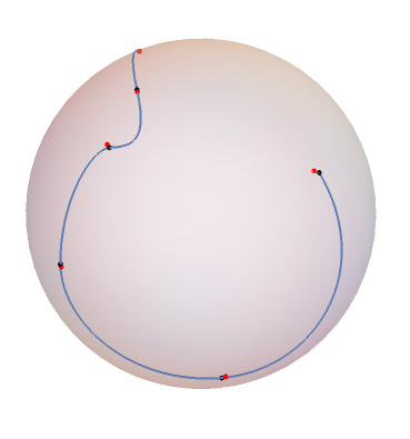
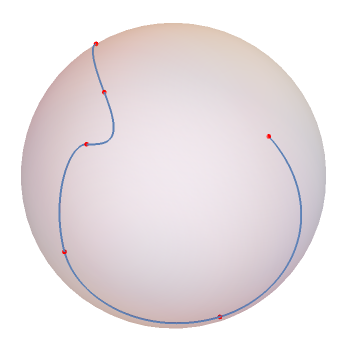
Figure 1. Curve in $\mathcal{D}^{1}(\mathbb{C}^{2})\equiv S^{2}$ for $\epsilon=0.005$ and 5 iterations of the algorithm (left) and 50 iterations (right). Points $\rho_{j}$ for $j=0,\ldots,5$ are represented in red. Points $\rho(t_{j})$ are represented in black. We see how on the right, target points and the points reached by the trajectory are indistinguishable. In the figure on the left we can see a small discrepancy between red and black points.

5. Example 2: the interpolation problem for a qutrit

As a second application of our method, this section presents the case of a three-level systems (a qutrit). The formulation is entirely analogous to the previous case but now the problem is formulated on the space $\mathcal{D}(\mathbb{C}^{3})\subset\mathfrak{u}^{*}(3)$. As we did in the qubit case we will use the identification of $\mathfrak{u}^{*}(3)$ with $\mathrm{i}\mathfrak{u}(3)$ and we will represent the density states as $3\times 3$ Hermitian matrices. As a basis, we will consider the set of Gell-Mann matrices

$$\lambda_{1}=\left(\begin{array}[]{ccc}0&1&0\\ 1&0&0\\ 0&0&0\\ \end{array}\right),\qquad\lambda_{2}=\left(\begin{array}[]{ccc}0&-i&0\\ i&0&0\\ 0&0&0\\ \end{array}\right),\qquad\lambda_{3}=\left(\begin{array}[]{ccc}1&0&0\\ 0&-1&0\\ 0&0&0\\ \end{array}\right)$$

$$\lambda_{4}=\left(\begin{array}[]{ccc}0&0&1\\ 0&0&0\\ 1&0&0\\ \end{array}\right),\qquad\lambda_{5}=\left(\begin{array}[]{ccc}0&0&-i\\ 0&0&0\\ i&0&0\\ \end{array}\right),\qquad\lambda_{6}=\left(\begin{array}[]{ccc}0&0&0\\ 0&0&1\\ 0&1&0\\ \end{array}\right)$$

$$\lambda_{7}=\left(\begin{array}[]{ccc}0&0&0\\ 0&0&-i\\ 0&i&0\\ \end{array}\right),\qquad\lambda_{8}=\frac{1}{\sqrt{3}}\left(\begin{array}[]{ccc}1&0&0\\ 0&1&0\\ 0&0&-2\\ \end{array}\right),\qquad\lambda_{9}=\sqrt{\frac{2}{3}}\left(\begin{array}[]{ccc}1&0&0\\ 0&1&0\\ 0&0&1\\ \end{array}\right).$$

The structure constants with respect to this basis are

$$c_{12}^{3}=-c_{21}^{3}=2;\quad c_{45}^{8}=c_{67}^{8}=-c_{54}^{8}=-c_{76}^{8}=\sqrt{3};$$

$$c_{14}^{7}=-c_{41}^{7}=-c_{15}^{6}=c_{51}^{6}=c_{24}^{6}=-c_{42}^{6}=c_{25}^{7}=-c_{52}^{7}=c_{34}^{5}=-c_{43}^{5}=c_{63}^{7}=-c_{36}^{7}=1$$

and zero otherwise. The elements $\rho\in\mathcal{D}(\mathcal{H})\subset\mathrm{i}\mathfrak{u}(3)$ are written as

$$\rho(t)=\frac{1}{2}\lambda_{9}+\sum_{k=1}^{8}x_{k}(t)\lambda_{k},$$ (46)

while the elements of the form $H\in T_{\rho}\mathrm{i}\mathfrak{u}(3)\sim\mathrm{i}\mathfrak{u}(3)$ become

$$H(t)=\sum_{k=1}^{9}y_{k}(t)\lambda_{k}.$$ (47)

With respect to these coordinates, we consider now the problem of finding the optimal control function $u(t)$ and the optimal state trajectory $(\rho(t),H(t))$ that minimizes the functional

$$J(u)=\int_{0}^{1}\frac{1}{2}\|u\|^{2}\,\mathrm{d}t+\frac{1}{2\epsilon}\sum_{j=1}^{N}\|\rho(t_{j})-\rho_{j}\|^{2}$$ (48)

and satisfies the dynamical system

$$\dot{\rho}(t)=-i(H(t)\rho(t)-\rho(t)H(t))\qquad\mbox{and}\qquad\displaystyle\dot{H}(t)=u(t),$$ (49)

subject to the initial conditions

$$\rho(0)=\rho_{0}\qquad\mbox{and}\qquad H(0)=\lambda_{9},$$ (50)

where regularity and interpolation conditions are assumed according to the dynamical interpolation problem $P$. As we saw above, we have to solve the system (37). Again, equations (34) imply that the value of $u(t)$ at the final point of each subinterval must vanish and this is imposed as a boundary condition. The value of $H(0)$ can also be seen to be irrelevant for the algorithm, as it happens in the case of two levels.

5.1. First example: points contained in a unitary orbit

Let us consider the following set of points, for times $t_{0}=0<t_{1}=\frac{1}{6}<t_{2}=\frac{1}{3}<t_{3}=\frac{1}{2}<t_{4}=\frac{2}{3}<t_{5}=\frac{5}{6}<t_{6}=1$:

$$\rho_{0}=\left(\begin{array}[]{ccc}\frac{1}{3}&0&0\\ 0&\frac{2}{3}&0\\ 0&0&0\\ \end{array}\right),$$

$$\rho_{1}=\left(\begin{array}[]{ccc}0.436919&-0.0234205-0.187994i&0.109777\,+0.158205i\\ -0.0234205+0.187994i&0.442465&0.0387764\,+0.0518969i\\ 0.109777\,-0.158205i&0.0387764\,-0.0518969i&0.120616\\ \end{array}\right),$$

$$\rho_{2}=\left(\begin{array}[]{ccc}0.25208&0.0710467\,-0.0594233i&-0.178472+0.143899i\\ 0.0710467\,+0.0594233i&0.358968&0.0437509\,-0.207081i\\ -0.178472-0.143899i&0.0437509\,+0.207081i&0.388953\\ \end{array}\right),$$

$$\rho_{3}=\left(\begin{array}[]{ccc}0.510032&0.0421306\,-0.160051i&-0.158675+0.163612i\\ 0.0421306\,+0.160051i&0.268756&0.0865724\,+0.0172119i\\ -0.158675-0.163612i&0.0865724\,-0.0172119i&0.221213\\ \end{array}\right),$$

$$\rho_{4}=\left(\begin{array}[]{ccc}0.145442&0.0762356\,-0.126603i&-0.0740697+0.211438i\\ 0.0762356\,+0.126603i&0.450398&-0.107868-0.0207668i\\ -0.0740697-0.211438i&-0.107868+0.0207668i&0.40416\\ \end{array}\right),$$

$$\rho_{5}=\left(\begin{array}[]{ccc}0.294447&0.1995\,-0.0726447i&-0.0696641+0.219691i\\ 0.1995\,+0.0726447i&0.301392&-0.0818337-0.0494491i\\ -0.0696641-0.219691i&-0.0818337+0.0494491i&0.40416\\ \end{array}\right),$$

$$\rho_{6}=\left(\begin{array}[]{ccc}0.0638338&-0.040794+0.00995446i&0.00664582\,-0.133158i\\ -0.040794-0.00995446i&0.522085&0.152599\,-0.104391i\\ 0.00664582\,+0.133158i&0.152599\,+0.104391i&0.414082\\ \end{array}\right).$$

All seven points belong to a unitary orbit of the set of mixed states in $\mathcal{D}(\mathbb{C}^{3})$.

We have considered again our algorithm for this case in order to verify how does it work for the case of mixed states. We have considered a value for $\epsilon=0.001$ and 200 iterations of our algorithm. The resulting distances of the points obtained and the values of the functional $J$ and its continuous part $J_{cont}$ are the following:

$t$	$\|\rho(t_{j})-\rho_{j}\|$	$J_{cont}$	$J$
$0$	$0$	0	0
$\frac{1}{6}$	$4.87\times 10^{-10}$	$1.82\times 10^{-16}$	$3.01\times 10^{-16}$
$\frac{1}{3}$	$6.7\times 10^{-4}$	$845.53$	$845.53$
$\frac{1}{2}$	$9.01\times 10^{-7}$	$607.02$	$607.02$
$\frac{2}{3}$	$9.51\times 10^{-9}$	$77.55$	$77.55$
$\frac{5}{6}$	$5.64\times 10^{-7}$	$298.54$	$298.54$
$1$	$8.9\times 10^{-6}$	$282.83$	$282.83$

Computation times are now longer, up to 5-6 seconds per iteration in certain cases. We conclude thus that the algorithm is also very efficient in the case of mixed states, although smaller values of the parameter $\epsilon$ must be considered. Notice that this example constitutes an important generalization with respect to the approach presented in [9] which makes sense only for pure states.

5.2. Points in different unitary orbits

Furthermore, the richness of the structure of unitary orbits of the set $\mathcal{D}(\mathbb{C}^{3})$ allows us to consider different situations. For instance, we can consider a case where the target points do not belong to the same unitary orbit and check the behavior of the algorithm. If we consider as initial point

$$\rho_{0b}=\left(\begin{array}[]{ccc}\frac{1}{3}-0.001&0&0\\ 0&\frac{2}{3}+0.001&0\\ 0&0&0\\ \end{array}\right),$$

and seek for a curve joining $\rho_{0b}$, $\rho_{1}$ and $\rho_{2}$ by using equations (37) we obtain points which are contained in the unitary orbit of $\rho_{0b}$. Hence, as $\rho_{1}$ and $\rho_{2}$ lie in a different orbit, the curve can not reach them. Nonetheless, the algorithm stabilizes (after 100 iterations) at points

$$\rho_{1b}=\left(\begin{array}[]{ccc}0.437204&-0.0233546-0.18881i&0.109899\,+0.158095i\\ -0.0233546+0.18881i&0.442331&0.0383441\,+0.0521308i\\ 0.109899\,-0.158095i&0.0383441\,-0.0521308i&0.120465\\ \end{array}\right)$$

and

$$\rho_{2b}=\left(\begin{array}[]{ccc}0.251872&0.070592\,-0.0598828i&-0.178803+0.143833i\\ 0.070592\,+0.0598828i&0.358735&0.0435776\,-0.207622i\\ -0.178803-0.143833i&0.0435776\,+0.207622i&0.389393\\ \end{array}\right)$$

which are at a distance of 0.001 of $\rho_{1}$ and $\rho_{2}$, respectively. These are the closest possible points since the unitary transformation must preserve the distance between both unitary orbits which is 0.001 at the initial points ($\rho_{0}$ and $\rho_{0b}$).

We conclude thus that our method provides an efficient numerical solution for the interpolation problem of general (pure or mixed) quantum states and generates a trajectory contained in the closest unitary orbit to them.

6. Conclusions and outlook

In this paper we have generalized the notion of quantum spline introduced in [9] to the case of general quantum states, pure or mixed. Brody et al. formulated a variational problem on a projective space defined in Section 1. They considered a globally defined continuous curve on the Lie group $U(n)$ and the corresponding set of continuous variations, and study the set of extremals of the functional defined in equation (1), which combines the curve on $U(n)$ and its action on the complex projective space. From this, they obtain a set of differential equations whose solutions correspond to Riemannian cubic polynomials on the subintervals $]t_{j-1},t_{j}[$ and a set of boundary conditions on the times $\{t_{j}\}$. Finding a global solution is a difficult problem and they also provide a numerical algorithm illustrated by a particular example in the case of a two level system.

Our definition reconsiders the problem and writes it on the complete set of quantum states (pure and mixed), modeled as a submanifold $\mathcal{D}$ of the dual space $\mathfrak{u}^{*}(n)$. Considering (as in [9] ) the case of unitary dynamics, allows us to forget about $\mathcal{D}$ and define the problem globally on the linear space $\mathfrak{u}^{*}(n)$. This simplifies the problem in a remarkable way. Furthermore, we consider a different type of optimization problem and choose a local formulation on the different subintervals of the time domain which does not impose the differentiability of the time dependence of the Hamiltonian. This choice, which is common, for instance, in quantum control solutions based on pulses, simplifies further the problem from the mathematical point of view, and transform it in a chain of Bolza-type problems. We consider then a Hamiltonian formulation of the corresponding control problem based on Pontryagin Maximum Principle, which allows us to consider in a natural way symplectic integrators associated to the geometrical formulation of Quantum Mechanics. Despite the much simpler formulation, the resulting system of differential equations is still difficult to solve exactly. We have introduced then an iterative algorithm to determine good solutions of the problem which works very efficiently for pure states and for mixed states, even for problems where the points to be interpolated do not belong to the same unitary orbit. Our algorithm allows us to define the closest unitary orbit in an efficient way.

Another advantage of our formalism is that it admits further generalizations in a simple way. Indeed, we can consider an analogous formulation where unitary dynamics is replaced by more general master equations, as for instance the Lindblad-Kossakowski equation. This Markovian generalization may impose some extra constraints on the set of possible times and points to be interpolated, but the formulation of the problem makes perfect sense. The conclusions of that analysis, which is being done now, will be presented in a future paper.

References

- [1] Abraham R and Marsden J E 1978 Foundations of Mechanics (Reading, MA: Addison-Wesley)
- [2] Altafini, C 2002 Modeling and Control of Quantum Systems: An Introduction IEEE Trans. Autom. Control, 57 (8), pp 1898-1917
- [3] Altafini, C 2003 Controllability properties for finite dimensional quantum Markovian master equations Journal of Mathematical Physics, 44, pp 2357-2372
- [4] Ashtekar A and Schilling T A 1998 Geometrical Formulation of Quantum Mechanics On Einstein’s Path: Essays in Honor of Engelbert Schucking ed A Harvey (Berlin: Springer-Verlag) pp 23–65
- [5] Bartana A and Kosloff, R 1993 Laser cooling of molecular internal degrees of freedom by a series of shaped pulses J. Chem. Phys. 99 (1) pp. 196
- [6] Bartana A and Kosloff, R 1997 Laser cooling of internal degrees of freedom. II J. Chem. Phys. 106 (4) pp. 1435
- [7] Breuer H P and Petruccione F 2002 The Theory of Open Quantum Systems (Oxford University Press)
- [8] Brody D C and Hughston L P 2001 Geometric quantum mechanics J. Geom. Phys. 38 19–53
- [9] Brody D C, Holm D D and Meier D M 2012 Quantum splines Phys. Rev. Letters 109 100501
- [10] Cariñena J F, Clemente-Gallardo J and Marmo G 2007 Geometrization of quantum mechanics Theoret. and Math. Phys. 152 (1) 894–903
- [11] Cesari L 1983 Optimization - Theory and Applications (Springer-Verlag)
- [12] Colombo, L, and de Diego, D M 2014 Higher-order variational problems on Lie groups and optimal control applications. J. Geom. Mech, 6(4), 451-478.
- [13] Crouch P and Silva Leite F 1995 The dynamic interpolation problem: On Riemannian manifolds, Lie groups, and symmetric spaces J. Dyn. Control Syst. 1 (2) 177–202
- [14] Dieci L, Russell R D and Vleck E S van 1994 Unitary integrators and applications to continous orthonormalization techniques SIAM J. Numerical Analysis 31 (1) 261-281
- [15] Gay-Balmaz F, Holm D D, Meier D M, Ratiu T S and Vialard F X 2012 Invariant higher-order variational problems. Communications in Mathematical Physics, 309(2), 413-458.
- [16] Grifoni M and Hänggi, P 1998 Driven quantum tunneling Phys. Rep. 304, pp 229-354
- [17] Hairer E, Lubich C and Wanner G 2006 Geometric numerical integration: structure-preserving algorithms for ordinary differential equations (Springer-Verlag Berlin Heidelberg)
- [18] Khaneja N, Brockett R and Glaser S Time optimal control in spin systems Phys. Rev. A 63 (2001) 032308
- [19] Kibble T 1979 Geometrization of quantum mechanics Comm. Math. Phys. 65 (2) 189–201
- [20] Konstant, B 1970 Quantization and unitary representations in Lectures in Modern Analysis and Applications III, Editors C. T. Taam, Springer, pp 87-208
- [21] Noakes L, Heinzinger G and Paden B 1989 Cubic splines on curved spaces IMA J. Math. Control Inform. 6 465–473
- [22] Ohtsuki, Y 1999 Monotonically convergent algorithm for quantum optimal control with dissipation J. Chem. Phys. 110 pp 9825
- [23] Werschnik J and Gross EKU 2007 Quantum optimal control theory J. Phys. B: At. Mol. Opt. Phys 40, R175-R211
- [24] Time optimal control of finite quantum systems J. Math. Phys. 41 5262
- [25] Whu W, Botina J and Rabitz H 1998 Rapidly convergent iteration methods for quantum optimal control of population J. Chem. Phys. 108 1953
- [26] Whu W and Rabitz H 1998 A rapid monotonically convergent iteration algorithm for quantum optimal control over the expectation value of a positive definite operator J. Chem. Phys. 109 385