Distributing CV entanglement over 4 co-propagating orthogonal modes

Abstract

We propose a scheme for distributing continuous variable entanglement originally established among a pair of mode between a set of four orthogonal co-propagating modes. This is accomplished by exploiting the possibility of coupling polarization with optical angular momentum provided by the q-plate. Here we present the principle of the proposed scheme with a short feasibility study that shows that the four-modes covariance matrix at the scheme output represent an entangled multi mode system.

1 Introduction

One of the most peculiar traits of quantum systems is the presence of correlations that cannot be explained by classical laws of physics. In continuous variable (CV) quantum optics this translates into squeezing for single field mode Wu86 and entanglement between distinct modes Ou92 .

Entanglement, firstly introduced by Schrödinger Schrodinger1935 in response to the famous Einstein, Podolsky, and Rosen (EPR) paper in 1935 EPR , plays a leading role for what concerns applications indeed, together with coherence and superposition, they are fundamental as quantum technology as emerged as the strategy to find enhanced ways of manipulating and transmitting information QuantumRev or to overcome the classical limits in measurements Quantum Metrology .

Here we will deal with CV entanglement in non-zero Orbital Angular Momentum (OAM) beams. OAM represents a discrete quantum variable (DV) spanning an infinite dimensional Hilbert space. Mixing CV systems with DV features allows achieving quantum tasks not accessible with either photon-number states or CV entanglement VanLoock2011 ; Andersen2015 .

In Ref. Pecoraro we reported on the preparation and the complete experimental characterization of a bipartite two-mode CV Gaussian entangled state carrying OAM.

In the present paper, we propose a scheme for distributing the entanglement, originally cast among a pair of modes in a type–II OPO, among a set of four mutually orthogonal modes. This is possible by exploiting the higher dimensionality provided by OAM. As a matter of fact, the use of a q-plate, a liquid crystal device that couples polarization with OAM Marrucci2006 , can realise a quantum beam-splitter among co-propagating modes that acquire multi-distinguishability thanks to the twofold label (polarization and OAM). In this way it is possible to distribute entanglement between co-propagating modes that are mutually orthogonal. The so obtained 4–modes Gaussian state is described by a 8x8 covariance matrix in phase space. Analysing the full system covariance matrix it can be found that a single q-plate allows to distribute entanglement between the four output modes creating three possible combination of pairs of entangled modes. This happens at the expense of introducing fictitious losses at the single mode level while preserving the total energy of the system.

The paper is structured as follows. In Sect. 2 we describe the action of a q-plate onto a pair of orthogonally polarised modes. Then, in Sect. 3, the manipulation of the entangled state at the output of a type–II non-degenerate OPO is detailed. Section 4 discusses the properties of the set of four modes at the q-plate output while conclusions are, eventually, drawn in Sect. 5.

2 The q-plate action

The q-plate is a liquid crystal device that couples polarization (bi-dimensional) d.o.f. with the infinite Hilbert space of optical orbital angular momentum (OAM).

A beam transmitted through a q-plate gains $2q$ quanta of OAM where the $q$ parameter is the topological charge of the device. The q-plate is composed of a thin liquid crystal film sandwiched between two glasses. The device is birefringent where $\delta$ is the retardation between the two axes. The retardation $\delta$ can be tuned by applying an alternate voltage to the liquid crystal cell.

OAM is an important property of light known since classical electromagnetic theory. Light, besides carrying energy, can also transport momentum in its linear and angular components. In particular, by focusing on the angular part, it’s possible to distinguish between the so-called spin angular momentum (SAM), macroscopically associated with polarization, and the orbital angular momentum (OAM) associated to the helicity of the phase fronts.

Both classical properties of light are kept all the way down to the single photon level and so to the quantum regime. They arise from solving the Helmholtz equation in paraxial approximation unveiling intrinsic properties of single photons.

More in detail, solving the most general form of the Helmholtz equation gives particular kinds of beams, such as Laguerre–Gauss ones, that are characterized by an azimuthal phase factor $e^{im\varphi}$ winding around the propagation axes. In this case, the beam acquires a peculiar helical wavefront, and shows, in a transverse plane, a doughnut intensity profile with an optical vortex at the centre due to the therein located phase singularity PadgettOAM ; OAMRev .

The value $\left|m\right|$ indicates that each photon in the beam carries $\left|m\right|$ quanta of OAM. Since in principle $m$ can assume any positive and negative integer value, this internal d.o.f. of the photon exploits an infinite dimensional Hilbert space allowing the possibility of encoding a large amount of informations onto a single beam.

Given at the q-plate input a generic k mode of orbital order m, its action, in the $L$ (left) and $R$ (right) circularly polarisation base, is:

$$\hat{Q}\;k_{\left[L,m\right]}=\cos\frac{\delta}{2}\;k_{\left[L,m\right]}+i\sin\frac{\delta}{2}\;k_{\left[R,m+2q\right]}$$

$$\hat{Q}\;k_{\left[R,m\right]}=\cos\frac{\delta}{2}\;k_{\left[R,m\right]}+i\sin\frac{\delta}{2}\;k_{\left[L,m-2q\right]}$$ (1)

where $\hat{Q}$ represents the q-plate operator, and $\left[A,m\right]$ labels the mode with OAM $m$ and polarization $A=(L,R)$.

From Eq. (1) it is easy to see that a q-plate couples polarization with OAM. In particular, entering the device with a circularly polarised light beam and a well defined OAM order m, gives raise to a pair of beams that are distinguishable for both d.o.f.. Tuning the birefringence retardation $\delta$ allows to change the weights of the output components and, in particular, setting $\delta=\pi$ a single circularly polarised beam travelling across the q-plate reverses its polarization and acquires $\pm 2q$ quanta of OAM. This regime has been exploited for endowing a cross polarised pair of CV entangled beams with OAM extra–distinguishability through the q-plate action as reported in Pecoraro .

Classically the q-plate acts as a device with one input and two outputs. From the quantum point of view this would be in contrast with the preservation of the Heisenberg uncertainty principle. From the quantum perspective, the q-plate is analogous to a beam–splitter acting onto the SAM+OAM mode space. As it will be detailed in the next section it couples two input mode to two output modes. The quantum action of the q-plate must take into account the vacuum modes that take part into the complete transformation. In particular, tuning the retardation $\delta$ to $\pi/2$ realise a balanced beam splitter acting on co-propagating orthogonal modes.

3 Manipulating a bi–partite CV polarization entangled state

Our starting point is a CV Gaussian bipartite two-mode entangled state generated by a type–II Optical Parametric Oscillator (OPO) working in frequency degeneration DAuria08 . Such a device generates two entangled frequency-degenerate continuous-wave beams exploiting the polarization as the distinguishing degree of freedom (d.o.f) DAuria09 . These two beams are in the fundamental a Gaussian mode ($TEM_{00}$), have linear orthogonal polarization and are collinear.

Let’s indicate these two modes with $a_{\left[H,0\right]}$ and $b_{\left[V,0\right]}$ ($\left[H,0\right]$ and $\left[V,0\right]$ are the polarization and the initial OAM value for the respective mode).

The scheme we are going to discuss in some details is sketched in Fig. 1.

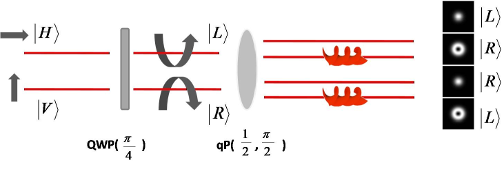
Figure 1: Scheme for the distribution of bipartite entanglement among four distinct orthogonal modes at the ouput of a type–II OPO. The initial orthogonally lineraly polarized pair pass through a quarter-waveplate for getting into an orthogonally circularly polarised pair. Then, passing through a properly tuned q-plate allows to access four modes distinguishable by either polarization and/or optical OAM.

The first step toward the distribution of the entanglement over four distinct modes is the use of a quarter-waveplate to makes the two OPO output beams circularly polarized so that $a_{\left[H,0\right]}\rightarrow a_{\left[L,0\right]}$ and $b_{\left[V,0\right]}\rightarrow b_{\left[R,0\right]}$.

Then, the two circularly polarised beams enters a $q=1/2$ q-plate tuned at $\delta=\pi/2$. To have a quantum picture of the q-plate induced transformation we have to consider a reversible version of Eq. (1). In order to obtain these relations we have to consider a transformation that involves, since the input, the 4 modes with labels $\left(\left[R,0\right],\left[L,0\right],\left[R,1\right],\left[L,-1\right]\right)$. The fully quantum version for Eq. (1) is

$$\hat{Q}\;a_{\left[L,0\right]}=\frac{1}{\sqrt{2}}\left(a_{\left[L,0\right]}+i\,a_{\left[R,1\right]}\right)$$

$$\hat{Q}\;a_{\left[R,1\right]}=\frac{1}{\sqrt{2}}\left(a_{\left[R,1\right]}+i\,a_{\left[L,0\right]}\right)$$

$$\hat{Q}\;b_{\left[R,0\right]}=\frac{1}{\sqrt{2}}\left(b_{\left[R,0\right]}+i\,b_{\left[L,-1\right]}\right)$$

$$\hat{Q}\;b_{\left[L,-1\right]}=\frac{1}{\sqrt{2}}\left(b_{\left[L,-1\right]}+i\,b_{\left[R,0\right]}\right)$$ (2)

It is straightforward to see that the above set of equations is made of two uncoupled sub-sets. For distinguishing the mode in and out from the q-plate, from now on we will identify the set of modes at the output by:

$$a_{1} \equiv a_{[L,0]}$$

$$a_{2} \equiv a_{[R,1]}$$

$$b_{1} \equiv b_{[R,0]}$$

$$b_{2} \equiv b_{[L,-1]}$$ (3)

Thanks to the introduction of OAM d.o.f. these modes are all orthogonal and so physically distinguishable.

In order to investigate the presence of mutual correlations among the set of output modes, we exploit the fact that the state produced by the OPO source is Gaussian i.e. it possesses a Gaussian Wigner function in phase space Olivares ; Gaussian . Hence, thanks to the Gaussian character, that is preserved by linear transformations as (2), the state of the four modes system can be completely characterized by its Covariance Matrix (CM) that, in this case, is a $8\times 8$ symmetric positive-definite matrix. To construct the state CM let us introduce pair of canonical quadrature operators i.e. for each mode of the set:

$$X_{k_{i}}=\frac{k_{i}+k_{i}^{\dagger}}{\sqrt{2}}$$

$$Y_{k_{i}}=\frac{k_{i}-k_{i}^{\dagger}}{\sqrt{2}i}$$

where $k=a,b$ and $i=1,2$. The second statistical moments of these two operators are the elements of the CM,

$$\Sigma_{4}=\left(\begin{array}[]{cccc}\sigma_{a_{1}}&\varepsilon_{12}&\varepsilon_{13}&\varepsilon_{14}\\ \varepsilon_{12}^{T}&\sigma_{a_{2}}&\varepsilon_{23}&\varepsilon_{24}\\ \varepsilon_{13}^{T}&\varepsilon_{23}^{T}&\sigma_{b_{1}}&\varepsilon_{34}\\ \varepsilon_{14}^{T}&\varepsilon_{24}^{T}&\varepsilon_{34}^{T}&\sigma_{b_{2}}\end{array}\right)$$ (4)

where the $\sigma$ blocks are single mode CM while $\varepsilon$ blocks contain information on the possibly quantum mutual correlation between distinct modes. They are given by:

$$\sigma_{k_{i}}=\left(\begin{array}[]{cc}\triangle X_{k_{i}}^{2}&\triangle X_{k_{i}}Y_{k_{i}}\\ \triangle Y_{k_{i}}X_{k_{i}}&\triangle Y_{k_{i}}^{2}\end{array}\right) \varepsilon_{ij}=\left(\begin{array}[]{cc}\triangle X_{k_{i}}X_{l_{j}}&\triangle X_{k_{i}}Y_{l_{j}}\\ \triangle Y_{k_{i}}X_{l_{j}}&\triangle Y_{k_{i}}Y_{l_{j}}\end{array}\right)$$ (9)

where $\triangle A_{k_{i}}^{2}$ are quadrature variances while covariance $\triangle A_{k_{i}}B_{l_{j}}$ are expressed as

$$\triangle A_{k_{i}}B_{l_{j}}=\frac{1}{2}\left\langle\left\{A_{k_{i}},B_{l_{j}}\right\}\right\rangle-\left\langle A_{k_{i}}\right\rangle\left\langle B_{l_{j}}\right\rangle$$

The presence of entanglement among pair of modes can be witnessed by applying suitable criteria to the elements of this matrix. A necessary and sufficient criterion for the (non–)separability of bipartite Gaussian states with an arbitrary number of modes has been established by Giedke et al. lewenstein . We will adopt this criterion later on to verify the presence of entanglement between realistic covariance matrices obtained transforming a pair of modes at the OPO output.

4 Properties of the four modes state

Let’s now focus on the quadrature of the modes at the q-plate output to properly construct the final CM with respect to the CM characterizing the pair of modes at the OPO output. As seen the set 2 can be split in two pairs descending from the OPO mode $a_{[H,0]}$ and $b_{[V,0]}$ respectively.

Inverting the first two Eqs. 2 one obtains

$$a_{1}=\frac{1}{\sqrt{2}}\left(a_{[L,0]}-i\tilde{a}_{[R,1]}\right)$$

$$a_{2}=\frac{1}{\sqrt{2}}\left(\tilde{a}_{[R,1]}-ia_{[L,0]}\right)$$ (10)

So that the relations among the quadratures of the two sides of the q-plate are:

$$X_{a_{1}}=\frac{1}{\sqrt{2}}\left(a_{1}+a_{1}^{\dagger}\right)=\frac{1}{\sqrt{2}}\left(X_{a_{[L,0]}}+\tilde{Y}_{a_{[R,1]}}\right)$$

$$Y_{a_{1}}=\frac{1}{\sqrt{2}i}\left(a_{1}-a_{1}^{\dagger}\right)=\frac{1}{\sqrt{2}}\left(Y_{a_{[L,0]}}-\tilde{X}_{a_{[R,1]}}\right)$$

$$X_{a_{2}}=\frac{1}{\sqrt{2}}\left(a_{2}+a_{2}^{\dagger}\right)=\frac{1}{\sqrt{2}}\left(\tilde{X}_{a_{[R,1]}}+Y_{a_{[L,0]}}\right)$$

$$Y_{a_{2}}=\frac{1}{\sqrt{2}i}\left(a_{2}-a_{2}^{\dagger}\right)=\frac{1}{\sqrt{2}}\left(\tilde{Y}_{a_{[R,1]}}-X_{a_{[L,0]}}\right)$$ (11)

Similarly, for the pair of mode coming from $b_{[V,0]}$ one gets:

$$b_{1} = \frac{1}{\sqrt{2}}\left(b_{[R,0]}-i\tilde{b}_{[L,-1]}\right)$$

$$b_{2} = \frac{1}{\sqrt{2}}\left(-ib_{[R,0]}+\tilde{b}_{[L,-1]}\right)$$ (12)

and the relations among quadratures are:

$$X_{b_{1}}=\frac{1}{\sqrt{2}}\left(b_{1}+b_{1}^{\dagger}\right)=\frac{1}{\sqrt{2}}\left(X_{b_{[R,0]}}+\tilde{Y}_{b_{[L,-1]}}\right)$$

$$Y_{b_{1}}=\frac{1}{\sqrt{2}i}\left(b_{1}-b_{1}^{\dagger}\right)=\frac{1}{\sqrt{2}}\left(Y_{b_{[R,0]}}-\tilde{X}_{b_{[L,-1]}}\right)$$

$$X_{b_{2}}=\frac{1}{\sqrt{2}}\left(b_{2}+b_{2}^{\dagger}\right)=\frac{1}{\sqrt{2}}\left(Y_{b_{[R,0]}}+\tilde{X}_{b_{[L,-1]}}\right)$$

$$Y_{b_{2}}=\frac{1}{\sqrt{2}i}\left(b_{2}-b_{2}^{\dagger}\right)=\frac{1}{\sqrt{2}}\left(\tilde{Y}_{b_{[L,-1]}}-X_{b_{[R,0]}}\right)$$ (13)

If the initial bipartite two-mode state (of the pair $\left(a_{[H,0]},b_{[V,0]}\right)$) is described by a $2\times 2$ CM in the standard form, i.e.:

$$\Sigma_{2}=\left(\begin{array}[]{cccc}a&0&c_{1}&0\\ 0&a&0&c_{2}\\ c_{1}&0&b&0\\ 0&c_{2}&0&b\end{array}\right)$$ (14)

one finds that $\Sigma_{4}$ can be written in terms of the elements of $\sigma_{2}$ as

$$\Sigma_{4}=\frac{1}{2}\left(\begin{array}[]{cccccccc}a+sn&0&0&sn-a&c_{1}&0&0&-c_{1}\\ 0&a+sn&a-sn&0&0&c_{2}&c_{2}&0\\ 0&a-sn&a+sn&0&0&c_{2}&c_{2}&0\\ sn-a&0&0&a+sn&-c_{1}&0&0&c_{1}\\ c_{1}&0&0&-c_{1}&b+sn&0&0&sn-b\\ 0&c_{2}&c_{2}&0&0&b+sn&b-sn&0\\ 0&c_{2}&c_{2}&0&0&b-sn&b+sn&0\\ -c_{1}&0&0&c_{1}&sn-b&0&0&b+sn\end{array}\right)$$ (15)

where $sn$ refers to the shot noise of the vacuum modes $sn=\triangle\widetilde{X}_{b_{[L,-1]}}^{2}=\triangle\widetilde{Y}_{b_{[L,-1]}}^{2}=\triangle\widetilde{X}_{a_{[R,1]}}^{2}=\triangle\widetilde{Y}_{b_{[R,1]}}^{2}=1/2$.

To perform a realistic feasibility test we have applied the above transformations to the experimental matrix $\Sigma_{2}$ reported in Ref. Pecoraro and corrected for collection losses. The matrix so obtained represents the pure state as it is generated inside the OPO crystal and it is given by:

$$\sigma_{exp}=\left(\begin{array}[]{cccc}0.72\pm 0.05&0&0.51\pm 0.01&0\\ 0&0.72\pm 0.05&0&-0.51\pm 0.01\\ 0.51\pm 0.01&0&0.72\pm 0.05&0\\ 0&-0.51\pm 0.01&0&0.72\pm 0.05\end{array}\right)$$ (16)

Putting these values in the matrix (15) one obtains

$$\sigma_{4(exp)}=\left(\begin{array}[]{cccccccc}0.60&0&0&-0.10&0.25&0&0&-0.25\\ 0&0.60&0.10&0&0&-0.25&-0.25&0\\ 0&0.10&0.60&0&0&-0.25&-0.25&0\\ -0.10&0&0.60&0.60&-0.25&0&0&0.25\\ 0.25&0&0&-0.25&0.60&0&0&-0.10\\ 0&-0.25&-0.25&0&0&0.60&0.10&0\\ 0&-0.25&-0.25&0&0&0.10&0.60&0\\ -0.25&0&0&0.25&-0.10&0&0&0.60\end{array}\right)$$ (17)

We set a Mathematica routine to apply to the above matrix the the Giedke et al. iterative criterion proving the presence of entanglement between pairs of subsystems. In particular, each mode has two entangled companions. $a_{1}$ is entangled with $b_{1}$ and $b_{2}$ (and vice-versa), the same happens for $a_{2}$. On the contrary, $a_{1}$ and $a_{2}$ are separable and the same is for $b_{1}$ and $b_{2}$.

5 Conclusions

In conclusion we have proposed a scheme to distribute the entanglement between two e.m. modes produced by a standard type-II phase matching OPO source among four modes so realizing a bipartite four-modes entangled state. This goal has been accomplished thanks to the introduction of the OAM degree of freedom. Vortex modes have been obtained by a q-plate that, by properly tuning its parameter $\delta$ , permits to split each of the two initial entangled modes into two further modes distinguishable by both OAM and polarization d.o.f. so accessing a larger Hilbert space. The Gaussian OAM-carrying bipartite four-modes state obtained in this way, can be fully characterized by its CM whose form, in terms of the initial pair of modes has been calculated. We have used an experimentally measured matrix in order to show that this scheme would effectively generate a bipartite four-modes entangled state. The entanglement of the final matrix has been established applying criterion introduced by Giedke et al. lewenstein

References

- (1) Ling-An Wu, H. J. Kimble, J. L. Hall, and Huifa Wu, Generation of Squeezed States by Parametric Down Conversion Phys. Rev. Lett. 57:2520 (1986);
- (2) Z. Y. Ou, S. F. Pereira, H. J. Kimble, and K. C. Peng, Realization of the Einstein-Podolsky-Rosen paradox for continuous variables Phys. Rev. Lett. 68:3663 (1992);
- (3) E. Schrödinger, Discussion of Probability Relations between Separated Systems, Proc. Cambridge Philos. Soc. 31:555 (1935);
- (4) A. Einstein, B. Podolsky, and N. Rosen, Can Quantum-Mechanical Description of Physical Reality Be Considered Complete?, Phys. Rev. 47:777 (1935);
- (5) Samuel L. Braunstein and Peter van Loock, Quantum information with continuous variables, Rev. Mod. Phys. 77:513 (2005); Quantum communication Nicolas Gisin and Rob Thew Nature Photonics 1, pages 165–171 (2007);
- (6) Advances in quantum metrology Vittorio Giovannetti, Seth Lloyd, and Lorenzo Maccone, Advances in quantum metrology, Nature Photonics 5:222 (2011);
- (7) P. van Loock, Optical Hybrid Approaches to Quantum Information, Laser Photonics Rev. 5:167 (2011);
- (8) U. L. Andersen, J. S. Neergaard-Nielsen, P. van Loock, and A. Furusawa, Hybrid discrete- and continuousvariable quantum information, Nat. Phys. 11:713 (2015);
- (9) A. Pecoraro, F. Cardano, L. Marrucci and A.Porzio, Continuous-Variable Entangled States of Light carrying Orbital Angular Momentum, arXiv:1805.05105;
- (10) L. Marrucci, C. Manzo, and D. Paparo, Optical Spin-to-Orbital Angular Momentum Conversion in Inhomogeneous Anisotropic Media, Phys. Rev. Lett. 96:163905 (2006);
- (11) A. M.Yao,and M.JPadgett, Orbital angular momentum: origins, behavior and applications, Adv. Opt. Photon. 3:161204(2011);
- (12) H. Rubinsztein-Dunlop, A. Forbes, M. V. Berry, M. R. Dennis, D. L. Andrews, M. Mansuripur, C. Denz, C. Alpmann, P. Banzer, T. Bauer, E. Karimi, L. Marrucci, M. Padgett, M. Ritsch-Marte, N. M. Litchinitser, N. P. Bigelow, C. Rosales-Guzmán, A. Belmonte, J. P. Torres, T. W. Neely, M. Baker, R. Gordon, A. B. Stilgoe, J. Romero, A. G. White, R. Fickler, A. E. Willner, G. Xie, B. McMorran, and A. M. Weiner, Roadmap on structured light, J. Opt. 19:013001 (2017);
- (13) V. D’Auria, S. Fornaro, A. Porzio, E.A. Sete, and S. Solimeno, Fine tuning of a triply resonant OPO for generating frequency degenerate CV entangled beams at low pump powers, Applied Physics B, 91:309 (2008);
- (14) V. DAuria, S. Fornaro, A. Porzio, S. Solimeno, S. Olivares, and M. G. A. Paris, Full Characterization of Gaussian Bipartite Entangled States by a Single Homodyne Detector, Phys. Rev. Lett. 102:020502 (2009);
- (15) S. Olivares, Quantum optics in the phase space, The European Physical Journal Special Topics, 203:3 (2012);
- (16) A.Ferraro, S.Olivares, M.G.A.Paris, Gaussian States in quantum information, (Bibliopolis, Napoli, 2005).
- (17) G. Giedke, B. Kraus, M. Lewenstein, and J. I. Cirac, Entanglement Criteria for All Bipartite Gaussian States, Phys. Rev. Lett. 87:167904 (2001);