Note on linear response for interacting Hall insulators

Abstract.

We relate explicitly the adiabatic curvature-in flux space- of an interacting Hall insulator with nondegenerate ground state to various linear response coefficients, in particular the Kubo response and the adiabatic response. The flexibility of the setup, allowing for various driving terms and currents, reflects the topological nature of the adiabatic curvature. We also outline an abstract connection between Kubo response and adiabatic response, corresponding to the fact that electric fields can be generated both by electrostatic potentials and time-dependent magnetic fields. Our treatment fits in the framework of rigorous many-body theory, thanks to the gap assumption.

1. Introduction

The Hall conductance is given by an adiabatic curvature, related to the threading of two Aharonov-Bohm fluxes. This insight originated with Niu, Thouless and Wu [1], see also the work of Avron and Seiler in [2]. Over the past years, it inspired a mathematically rigorous proof [3] by Hastings and Michalakis of quantization in the integer quantum Hall effect in the many-body context.

The goal of this note is not to sketch these developments but rather to review why the adiabatic curvature is indeed a Hall response coefficient. This is hence not a new insight, but we found it quite useful to phrase it in the language of modern many-body theory, using tools like quasi-adiabatic evolution and the like.

A related question that one might want to see clarified is the rigorous justification of linear response per se. While in general this remains an important problem of mathematical physics, it is under control in the case of Hall responses (exactly because these are non-dissipative responses), see [4, 5, 6]. This issue will however not be discussed here.

2. Setup

2.1. Spaces and operators

We use very heavily the setup and notation from a recent paper of ours, namely [7]. We consider a two dimensional discrete torus $\Gamma=\Gamma_{L}={\mathbb{Z}}^{2}_{L}$ with ${\mathbb{Z}}_{L}={\mathbb{Z}}/(L{\mathbb{Z}})$. We take $L$ large and even and we often identify $\Gamma$ with the square $\{(x_{1},x_{2})\in{\mathbb{Z}}^{2}\;:\;-L/2\leq x_{1,2}\leq L/2\}$, with the appropriate identification of boundary points.

A finite-dimensional Hilbert space ${\mathbb{C}}^{n}$ is associated to each site $x\in\Gamma$ and there is a preferred basis in ${\mathbb{C}}^{n}$ labelled by $\sigma$ (as an example, one can think of the $z$-spin number). We consider the fermionic Fock space ${\mathcal{H}}={\mathcal{H}}_{\Gamma}$ built on the one-particle space $l^{2}(\Gamma,{\mathbb{C}}^{n})$. The algebra of operators ${\mathcal{B}}({\mathcal{H}})$ is generated by the creation/annihilation operators $c_{x,\sigma}/c^{*}_{x,\sigma}$:

$$\{c_{x,\sigma},c^{*}_{x^{\prime},\sigma^{\prime}}\}=\delta_{x,x^{\prime}}\delta_{\sigma,\sigma^{\prime}},\qquad\{c^{\sharp}_{x,\sigma},c^{\sharp}_{x^{\prime},\sigma^{\prime}}\}=0$$

where $\{A,B\}=AB+BA$ and $c^{\sharp}$ can be either $c$ or $c^{*}$. Any operator $O$ can be written in a unique way as a sum of normal-ordered monomials in $c^{\sharp}_{x,\sigma}$ which are at most of first degree in each $c^{\sharp}_{x,\sigma}$. Referring to this unique representation, we write $O_{S}$ for the ‘restriction to $S$’, namely the sum of monomials in $O$ containing only $c^{\sharp}_{x,\sigma}$ with $x\in S$.

For obvious reasons, we call $S$ the ‘spatial support’ of $O_{S}$. Also, we will consider only Hamiltonians and observables that are in the even subalgebra, i.e. they contain only monomials of even degree. A direct consequence of this is that, for even $O,O^{\prime}$ we have $[O_{S},O^{\prime}_{S^{\prime}}]=0$ whenever $S\cap S^{\prime}=\emptyset$. An oft-used operator is the particle number at $x$, given by $n_{x}=\sum_{\sigma}c^{*}_{x,\sigma}c_{x,\sigma}$ and the particle number in $X$, given by $n_{X}=\sum_{x\in X}n_{x}$.

We will in general write $S^{r}$ for the neighborhood

(2.1) $$S^{r}=\{x|\,\mathrm{\mathrm{dist}}(x,S)\leq r\}$$

Here the distance $\mathrm{\mathrm{dist}}(\cdot,\cdot)$ refers to the Euclidian distance on the underlying continuous torus $[-L/2,L/2]^{2}$ with opposite edges identified.

Consider an observable $O_{L}$ on $\Gamma_{L}$ whose support $S$ fits inside a smaller square, say $|x_{1,2}|\leq L/4$ for all $x\in S$, then we can define a corresponding $O_{L^{\prime}}$ on $\Gamma_{L^{\prime}}$ for $L^{\prime}>L$ by the identification of $\Gamma_{L}$ with a square. This realizes a natural embedding of ${\mathcal{B}}({\mathcal{H}}_{\Gamma_{L}})$ into ${\mathcal{B}}({\mathcal{H}}_{\Gamma_{L^{\prime}}})$. We will use this to fix an observable $O$ and consider it implicitly for all (sufficiently large) $L$. For example Assumption 2.2 relies on this construction.

We also need another class of operators, representing Hamiltonians, currents, etc. They are of the type $G=\sum_{X\in\Gamma}G_{X}$, with

1. $G_{X}=0$ unless $\mathrm{diam}(X)\leq R$ for some fixed range $R<\infty$.

2. $\left\|G_{X}\right\|\leq m$ for some fixed $m$.

For lack of a better name, we call (the $L$-sequence of) $G$ a ‘local Hamiltonian’ whenever the above conditions are satisfied for all $L$ with $m,R$ independent of $L$. Of course, one can devise a framework to consider ‘the same’ $G$ for different $L$, but we will not need this explicitly.

2.2. The Hamiltonian

Our framework allows to consider rather arbitrary local Hamiltonians, but for the sake of simplicity, we restrict to a class with nearest neighbour hopping:

$$H=\sum_{\sigma,\sigma^{\prime}}\sum_{x\sim x^{\prime}}\alpha(x,\sigma,x^{\prime},\sigma^{\prime})c^{*}_{x,\sigma}c_{x^{\prime},\sigma^{\prime}}+\sum_{X\subset\Gamma}B_{X}$$

where $x\sim x^{\prime}$ indicates that $x,x^{\prime}$ are adjacent, and

1. $\alpha(x,\sigma,x^{\prime},\sigma^{\prime})=\overline{\alpha(x^{\prime},\sigma^{\prime},x,\sigma)}$ to ensure Hermiticity.

2. $\sum_{X}B_{X}$ is a ‘local Hamiltonian’ as defined above in Section 2.1.

3. All $B_{X}$ are Hermitian and $[B_{X},n_{x}]=0$ for any $x,X$.

The conserved charge is $N=\sum_{x}n_{x}$, i.e. for simplicity we assume unit charge per fermion. By $\mathrm{iii})$, we see that the $B_{X}$ don’t contribute to charge transport. The natural choice for these $B_{X}$ is

$$B_{\{x\}}=\mu n_{x}+Un_{x}^{2},\qquad B_{X}=0\text{ if $|X|>1$}$$

i.e.  the Hubbard model with on-site interaction $U$ and chemical potential $\mu$. The main assumptions on the Hamiltonian are

Assumption 2.1.

$H$ has a non-degenerate ground state $\Psi$ separated from the rest of the spectrum by a distance ${g}>0$, uniformly in the size $L$.

Let us write $\omega(\cdot)=\langle\Psi,\cdot\Psi\rangle$ for the ground state expectation. Sometimes, as in the upcoming assumption, we need to recall that everything depends on $L$, so we may write $\omega(\cdot)=\omega_{L}(\cdot)$.

Assumption 2.2.

The ground state has a thermodynamic limit in a weak sense: for any observable $O$ with finite support, the limit $\lim_{L\to\infty}\omega_{L}(O)$ exists. (We used the identification in Section 2.1 of observables for different $L$ to give meaning to $\omega_{L}(O)=\omega_{L}(O_{L})$)

These assumptions are assumed to hold throughout our text and we do not repeat them. That being said, Assumption 2.2 is only necessary for Lemma 3.1 and Theorem 4.1. In all what follows, we always mean that error terms, constants $C$, etc can be taken bounded independently of $L$.

2.2.1. Example: interacting Harper model

We take $n=1$, i.e. spinless fermions, so we omit the label $\sigma$. The hopping amplitudes $\alpha$ are specified as

(2.2) $$\alpha(x,x^{\prime})=\begin{cases}t\mathrm{e}^{\pm\mathrm{i}\Phi_{L}x_{1}}&\qquad x_{1}=x^{\prime}_{1}\quad\text{and}\quad(x^{\prime}_{2}-x_{2})\mathrm{mod}L=\pm 1\\ t&\qquad x_{2}=x^{\prime}_{2}\quad\text{and}\quad(x^{\prime}_{1}-x_{1})\mathrm{mod}L=\pm 1\end{cases}$$

where $\Phi_{L}\in 2\pi{\mathbb{Z}}/L$ is the magnetic flux per unit cell and $t\in{\mathbb{R}}$ is the hopping strength. Note that $\Phi_{L}\in 2\pi{\mathbb{Z}}/L$ ensures that the hopping amplitudes are well defined on the $L\times L$ torus. The infinite volume Harper model[9] is well-defined for all values of the flux $\Phi$ and Lesbegue a.e. $\Phi$ satisfy the following property: there is an open set $U\ni\Phi$ and a chemical potential $\mu$ such that, for every $\Phi^{\prime}\in U$, $\mu$ lies outside of the spectrum of the Harper Hamiltonian. Let $\Phi$ satisfy this property, then we can find a sequence of fluxes $\Phi_{L}\rightarrow\Phi$ such that the corresponding sequence of finite-volume Harper models statisfies assumptions 2.1 and 2.2. So far the non-interacting model. Persistence of gaps for weak interactions was proven in [10, 11] and also implicitly in [5], and existence of the thermodynamic limit is standard in this context.

2.3. Fluxes

2.3.1. One-forms on $\Gamma$

We want to ‘thread magnetic fluxes’ through the loops of the torus $\Gamma$. These fluxes will be modelled using vector potentials, which we describe as discrete one-forms, i.e. objects that can be integrated along oriented paths. The elements of an oriented path are the oriented edges which it traverses. A one-form is a function $A:\Gamma^{e}\rightarrow{\mathbb{R}}$ on the oriented edges of $\Gamma$ such that $A(e)$ flips sign if the orientation of $e$ is reversed. We write $\left\|A\right\|:=\sup_{e}|A(e)|$.

The integral of $A$ along $\gamma$ is then

$$\int_{\gamma}A:=\sum_{e\in\gamma}A(e).$$

Any function $\theta:\Gamma\rightarrow{\mathbb{R}}$ defines a one-form $\mathrm{d}\theta$ by $\mathrm{d}\theta\big{(}(x,y)\big{)}=\theta(y)-\theta(x)$. See the appendix for more details on discrete one-forms.

2.3.2. Hamiltonian with vector potential

Vector potentials are one-forms $A$. A background vector potential $A$ is implemented by modifying the Hamiltonian in the following way:

$$H\to H_{A},\qquad\alpha(x,\sigma;x^{\prime},\sigma^{\prime})\to\alpha(x,\sigma;x^{\prime},\sigma^{\prime})\mathrm{e}^{\mathrm{i}A\big{(}(x,x^{\prime})\big{)}}.$$

In practice, we do not need any additional magnetic fluxes piercing the lattice, so we will mostly restrict to vortex-free $A$ i.e. $\oint_{\gamma}A=0$ across loops $\gamma$ that are contractible to a point. The implementation of a vector potential of the form $\mathrm{d}\theta$ for some function $\theta:\Gamma\to{\mathbb{R}}$ amouts to a gauge transformation

(2.3) $$U_{\theta}H_{A}U^{*}_{\theta}=H_{A+\mathrm{d}\theta}$$

where

$$U_{\theta}=\mathrm{e}^{\mathrm{i}\langle\theta,n\rangle},\qquad\langle\theta,n\rangle\equiv\sum_{x}\theta(x)n_{x}.$$

Consider now a one-form $A$ that is exact in the region $\Sigma\subset\Gamma$. By this we mean that $\oint_{\gamma}A=0$ for any $\gamma$, not necessarily contractible, consisting of oriented edges in $\Sigma^{e}$ (edges whose both vertices are in $\Sigma$). Then there exists a function $\theta$, with support in $\Sigma$, such that

$$A\big{|}_{\Sigma^{e}}={\mathrm{d}}\theta.$$

This in particular implies that

(2.4) $$(H_{A})_{\Sigma}=(U_{\theta}HU^{*}_{\theta})_{\Sigma}.$$

If we identify gauge equivalent vector potentials, then there are only two independent nonzero vortex-free classes. A representant of the first (second) class is given by the vector potential $\xi_{1}$ ($\xi_{2}$) which takes the value $1/L$ on edges pointing in the positive $1$-direction ($2$-direction), and vanishes on edges pointing in the $2$-direction ($1$-direction). The point is that locally the one-form $\xi_{i}$ is given by $\mathrm{d}x_{i}/L$.

Let $\gamma_{1},\gamma_{2}$ be two loops that wind around the torus across the lines $x_{2}=0,x_{1}=0$, respectively. Then

$$\int_{\gamma_{i}}\xi_{j}=\delta_{ij}.$$

Any vector potential of the form $\phi_{1}(\xi_{1}+\mathrm{d}\theta_{1})+\phi_{2}(\xi_{2}+\mathrm{d}\theta_{2})$ describes magnetic fluxes $(\phi_{1},\phi_{2})$ threaded through the torus, with no magnetic fields on the torus, see Figure  1

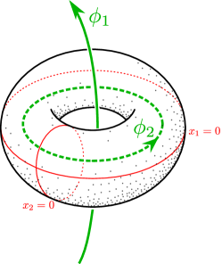
Figure 1. The torus $\Gamma$ with threaded fluxes $\phi_{1}$ and $\phi_{2}$.

2.4. Current operators

Let us define current, related to the flow of the conserved charge $N$. For any connected region $X\subset\Gamma$, the instantaneous change of $n_{X}$ is given by

$$J_{\partial X}=\mathrm{i}[H,n_{X}]$$

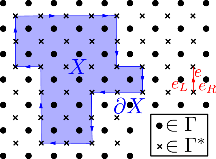
(a) The boundary of the set $X$ as an oriented path, and an edge $e$ together with the vertices $e_{L}$ and $e_{R}$ which it passes.

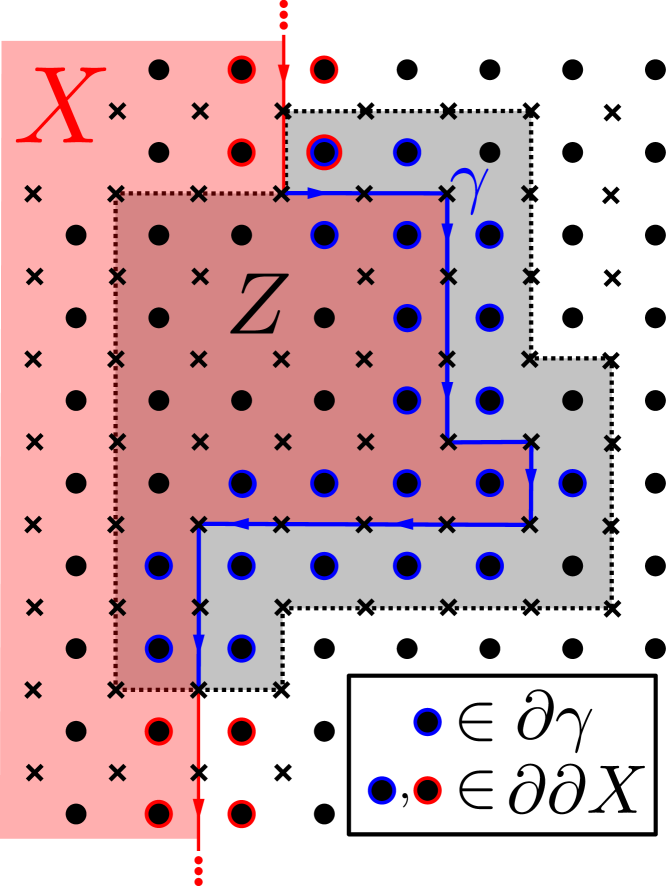
(b) The path $\gamma$ as a restriction of the boundary of $X$.

Figure 2.

and so it is natural to interpret $J_{\partial X}$ as the current operator through the non-intersecting oriented loop $\partial X$ in the dual lattice $\Gamma^{*}$. By convention, we orient $\partial X$ in a ‘counter-clockwise’ fashion, i.e. when walking along $\partial X$, one sees the set $X$ to the right, see Figure 2(a). Moreover, since $J_{\partial X}$ is a sum of local operators situated in a close vicinity of $\partial X$, we can also associate in a natural way a current $J_{\gamma}$ to every oriented subpath $\gamma$ of $\partial X$.

The ambiguity in doing this amounts to an operator of norm at most $C(R)$ at the ends of $\gamma$, with $R$ the range of the Hamiltonian (actually, only the range of the hopping term would enter here). Therefore, $J_{\gamma}$ will be meaningful whenever $|\gamma|\gg C(R)$. For the sake of explicitness, we give a possible choice. Note first that each oriented edge $e$ of $\Gamma^{*}$ is uniquely specified by giving the site $e_{L}$, which lies just to the left of $e$, and the site $e_{R}$, which lies just to the right of $e$. We set

$$J_{\gamma}=-\mathrm{i}\sum_{e\in\gamma}\left(\alpha(e_{L},e_{R})c_{e_{R}}^{*}c_{e_{L}}-\alpha(e_{R},e_{L})c_{e_{L}}^{*}c_{e_{R}}\right).$$

The formalism of gauge transformations offers us a handy way to write $J_{\gamma}$. Write $\partial\gamma:=\cup_{e\in\gamma}\{e_{L},e_{R}\}$ for the vertices passed by $\gamma$. The idea is to find a region $X$ such that $\gamma$ is a subpath of $\partial X$ and to write $J_{\gamma}$ as a (spatial restriction of) the current into $X$, i.e.

$$(J_{\partial X})_{Z}=J_{\gamma}$$

for a region $Z$ that selects exactly the right part of $\partial X$. To be precise, $Z$ has to satisfy $Z\supset\partial\gamma$ and $(\partial\partial X\setminus\partial\gamma)\cap Z=\emptyset$, see Figure 2(b).

Therefore we have also

(2.5) $$J_{\gamma}=\partial_{\phi}(\mathrm{e}^{\mathrm{i}\phi n_{X}}H\mathrm{e}^{\mathrm{i}\phi n_{X}})_{Z}\big{|}_{\phi=0}=\mathrm{i}([n_{X},H])_{Z}$$

which relates current operators to flux threading. The last equality is a consequence of the fact that the restriction to a spatial region is a linear map on operators.

3. Response coefficients

3.1. Kubo Linear response

The Kubo linear response coefficient $\chi_{J,V}(\nu)$ at frequency $\nu$, describes the response of an observable $J$ to adding a perturbation $\mathrm{e}^{\mathrm{i}\nu t}V$ to the Hamiltonian starting at $t=0$ [12]. We simply start from the well-known expression for the response coefficient:

(3.1) $$\chi_{J,V}(\nu):=\mathrm{i}\lim_{\epsilon\rightarrow 0^{+}}\int_{0}^{\infty}\mathrm{d}t\;\omega\left([V(-t),J]\right)\mathrm{e}^{\mathrm{i}\nu t-\epsilon t},\qquad\text{and $\chi_{J,V}=\chi_{J,V}(0)$}$$

where $V(t)=\mathrm{e}^{\mathrm{i}tH}V\mathrm{e}^{-\mathrm{i}tH}$. We should immediately add that it is often crucial to take the thermodynamic limit $L\nearrow\infty$ before taking $\epsilon\rightarrow 0^{+}$. However, for gapped systems (as we are considering) these limits commute:

Lemma 3.1.

Let $|\nu|\leq g/2$ (recall that $g$ is the spectral gap). If both $J,V$ are operators with finite support, then

(3.2) $$\mathrm{i}\lim_{\epsilon\rightarrow 0^{+}}\lim_{L\to\infty}\int_{0}^{\infty}\mathrm{d}t\;\omega\left([V(-t),J]\right)\mathrm{e}^{\mathrm{i}\nu t-\epsilon t}$$

exists and equals the $L\nearrow\infty$ limit of (3.1).

We will hence consider always (3.1) but we stress that the commutativity of limits exhibited in Lemma 3.1 actually precludes any dissipative effect.

One of the features of the Kubo response that we will rely on, is its locality, made explicit in the following lemma.

Lemma 3.2.

Let $|\nu|<g/2$. Let $J,V$ be local Hamiltonians in the sense of Section 2.1 and assume that the region $Z$ is the intersection of their supports. Then

(3.3) $$\chi_{J,V}(\nu)-\chi_{J_{Z^{r}},V_{Z^{r}}}(\nu)={\mathcal{O}}(r^{-\infty})$$

with $Z^{r}$ as defined in (2.1). Actually, $\chi_{J,V}=\mathrm{i}\>\omega([{\mathcal{I}}(J),V])$ (with ${\mathcal{I}}$ defined in Section 5.1) which renders this locality explicit.

3.2. Adiabatic response

Since this setup is less familiar to most readers, we sketch how it is derived from fundamental considerations. Consider a family of Hamiltonians $H_{s}$ for $s\in[-1,1]$ with uniformly gapped groundsates $\Psi_{s}$. We require that the map $s\mapsto H_{s}$ is smooth and that $\partial^{n}_{s}H_{s}=0$ at $s=-1$, for all $n$. Now, to put ourselves in the adiabatic regime, the parameter $s$ is varied slowly: the Hamiltonian in physical time $t$ is given by $H^{\epsilon}(t):=H_{\epsilon t}$. Write $\Psi^{\epsilon}_{t}$ for the solution to the time-dependent Schrödinger equation (TSE)

$$\mathrm{i}\>\partial_{t}\Psi^{\epsilon}_{t}=H^{\epsilon}(t)\Psi^{\epsilon}_{t},\qquad\text{with initial condition}\quad\Psi^{\epsilon}_{-1/\epsilon}=\Psi_{-1}.$$

The adiabatic response of some local observable $J$ at parameter $s$ is then defined as the difference between the solution of the TSE and the instantaneous ground state:

(3.4) $$\chi^{\mathrm{ad}}_{J,H_{s}}:=\lim_{\epsilon\rightarrow 0}\tfrac{1}{\epsilon}\left({\langle\Psi^{\epsilon}_{s/\epsilon},J\;\Psi^{\epsilon}_{s/\epsilon}\rangle-\langle\Psi_{s},J\;\Psi_{s}\rangle}\right).$$

Of course, the same remark about the thermodynamic limit as in Section 3.1 applies here and we do not comment on that further. From now on, we will always choose $s=0$ in (3.4). Let us give now heuristically evaluate (3.4). Since the state is close to the instantaneous ground state, let us pretend that they are exactly equal at time $t=0$ and evaluate the difference at $t\gg 1$, but $t$ not growing with $\epsilon$, such that $t/\epsilon$ still morally corresponds to taking $s=0$ in (3.4). In other words we look at

$$\lim_{t\to\infty}\;\lim_{\epsilon\rightarrow 0}\tfrac{1}{\epsilon}\left({\langle\Psi^{\epsilon}_{t},J\;\Psi^{\epsilon}_{t}\rangle-\langle\Psi_{0},J\;\Psi_{0}\rangle}\right),\qquad\text{started from}\quad\Psi^{\epsilon}_{0}:=\Psi_{0}$$

The advantage of doing so is that only the values of $H_{s}$ near $s=0$ seem to matter. We expand $H^{\epsilon}(t)$ around $t=0$, where $H^{\epsilon}(0)=H_{0}$, obtaining

(3.5) $$H^{\epsilon}(t)=H_{0}+(H^{\epsilon}(t)-H_{0})\approx H_{0}+\epsilon tW,\qquad W=\partial_{s}H_{s}\big{|}_{s=0}.$$

What we have gained is that the setup now looks very much like the setup of the Kubo response formula: We start at $t=0$ in the ground state and we switch on a time-dependent driving, with the time-dependence being linear. In this setup one derives the Kubo response formula by making a Dyson expansion of the dynamics, up to first order in $\epsilon$ and taking $t\to\infty$ (after introducing a regularization $\mathrm{e}^{-\delta t}$). Doing this, we arrive at

(3.6) $$\chi^{\mathrm{ad}}_{J,H_{s}}=\mathrm{i}\lim_{\delta\rightarrow 0^{+}}\int_{0}^{\infty}\mathrm{d}t\;t\omega\left([W(-t),J]\right)\mathrm{e}^{-\delta t}.$$

By standard Fourier techniques and renaming $\delta\to\epsilon$, this leads to

(3.7) $$\chi^{\mathrm{ad}}_{J,H_{s}}=\lim_{\epsilon\rightarrow 0^{+}}\frac{\partial}{\partial\nu}\int_{0}^{\infty}\mathrm{d}t\;\mathrm{e}^{\mathrm{i}\nu t}\omega\left([W(-t),J]\right)e^{-\epsilon t}\big{|}_{\nu=0}=-\mathrm{i}\frac{\partial}{\partial\nu}\chi_{J,W}(\nu)\big{|}_{\nu=0}$$

Therefore, this heuristic treatment suggests that the adiabatic response is directly related to the Kubo linear response. Indeed, using the adiabatic perturbation theory in [13], we have

Lemma 3.3.

Assume that Assumption 2.1 holds for all $s\in[-1,1]$ uniformly, that $H_{s}$ are local Hamiltonians whose parameters $m,R$ can be chosen uniformly in $s$ and that all local terms $H_{s,X}$ are smooth, uniformly in $X$. Then (3.6) holds true.

3.3. Adiabatic curvature

We recall the vector potential $A=\phi_{1}\xi_{1}+\phi_{2}\xi_{2}$ introduced in Section 2.3, corresponding to threaded fluxes $\phi=(\phi_{1},\phi_{2})$. We now consider the so-called twist Hamiltonians

$$H(\phi)=H(\phi_{1},\phi_{2})=H_{\phi_{1}\xi_{1}+\phi_{2}\xi_{2}},\qquad\phi\in{\mathbb{T}}^{2}.$$

For small $\phi$, the twist Hamiltonian $H(\phi)$ is a small (in norm) perturbation of $H$, so from assumption 2.1 it follows that we can find a neighbourhood ${\mathcal{U}}={\mathcal{U}}(L)$ of $\phi=0$ such that the twist Hamiltonian $H(\phi)$ also has a non-degenerate ground state, gapped by ${g}/2$. In this neighbourhood ${\mathcal{U}}$, we denote by ${P}(\phi)$ the ground state projection of ${H}(\phi)$. We thus have a two-parameter family of projections of which we consider the adiabatic curvature at $\phi=0$:

(3.8) $$\kappa:=\mathrm{i}\;\mathrm{Tr}\left({P}[\partial_{1}{P},\partial_{2}{P}]\right)=\mathrm{i}\;\omega\left([\partial_{1}{P},\partial_{2}{P}]\right),\qquad\partial_{i}P=\partial_{\phi_{i}}P(\phi)\big{|}_{\phi=0}$$

We immediately point out that $\kappa$ is independent of the precise form of the vector potential $A$ that was used to define the twist Hamiltonian. Indeed, consider another vortex-free $A^{\prime}$ that threads the same flux $(\phi_{1},\phi_{2})$, implying that it is of the form

$$A^{\prime}=\phi_{1}(\xi_{1}+\mathrm{d}\theta_{1})+\phi_{2}(\xi_{2}+\mathrm{d}\theta_{2})=A+\mathrm{d}f,\qquad\text{where}\quad f=\phi_{1}\theta_{1}+\phi_{2}\theta_{2}.$$

Then changing $A\to A^{\prime}$ does not change the adiabatic curvature $\kappa$. More precisely,

Lemma 3.4.

Let $H^{\prime}(\phi)$ be

$$H^{\prime}(\phi)=H_{A^{\prime}},\qquad A^{\prime}=\phi_{1}(\xi_{1}+\mathrm{d}\theta_{1})+\phi_{2}(\xi_{2}+\mathrm{d}\theta_{2})$$

for some functions $\theta_{1,2}$ satisfying $\left\|\mathrm{d}\theta_{1,2}\right\|\leq C$. By (2.3) these Hamiltonians are also uniformly gapped for $\phi$ in a neighbourhood ${\mathcal{U}}^{\prime}$ of $0$. If we write $P^{\prime}(\phi)$ for the corresponding groundstate projections, then

$$\kappa=\mathrm{i}\>\omega^{\prime}\left([\partial_{1}P^{\prime},\partial_{2}P^{\prime}]\right)+{\mathcal{O}}(L^{-\infty}).$$

It is useful to state an alternative, oft-used form of the curvature. Its basic ingredients are generators of parallel transport $K_{i}$. These operators have to satisfy the relation

(3.9) $$\partial_{j}P=\mathrm{i}\>[K_{j},P],\qquad j=1,2.$$

It is immediate that this relation does not fix $K_{i}$ uniquely. A choice that one encounters often (but that is rather useless in the many-body setting because it is not local) is $K_{i}=P(\partial_{i}P)(1-P)+(1-P)(\partial_{i}P)P$. By a little algebra, we see that

(3.10) $$\omega([[K_{1},P],[K_{2},P]])=-\omega([K_{1},K_{2}])$$

and hence, for any pair $K_{1,2}$ of generators of parallel transport,

$$\kappa=\mathrm{i}\>\omega([K_{1},K_{2}]).$$

4. Results

To put the results that follow into a firm context, we note that a strong from of quantization was proven in [3, 14, 5] for the adiabatic curvature $\kappa$ as introduced in Section 3.3, namely,

Theorem 4.1.

There exists $n\in{\mathbb{Z}}$ such that

$$\left|\kappa-2\pi n\right|={\mathcal{O}}(L^{-\infty}).$$

Note that the proof of this theorem is simplified if one demands that Assumption 2.1 holds for all fluxes $\phi\in{\mathbb{T}}^{2}$, see [7]. In view of this result, we build up the following sections as linking alternatively defined response coefficients to $\kappa$.

4.1. From the Kubo response to adiabatic curvature

We want to compute the current density in response to a perpendicular applied electric field. We measure this current density $j_{2}$ in the $2$-direction and at the origin. The driving is by a uniform electric field of strength $E$ in the $1$-direction. The Hall conductivity in this setup should be

(4.1) $$\frac{j_{2}}{E}=\frac{\langle J_{\gamma_{d}}\rangle}{2dE},\qquad E\to 0$$

where $\gamma_{d}$ is the oriented path in $\Gamma^{*}$ running in the $x_{1}$-direction from $-d+1/2$ to $d+1/2$ at $x_{2}=1/2$ i.e. it has length $2d$, see Figure 3. The corresponding current operator $J_{\gamma_{d}}$ was defined in Section 2.4. To implement the electric field, we choose an electrostatic potential $v$ that gives a constant electric field in the strip $\{|x_{1}|\leq\ell\}$:

(4.2) $${\mathrm{d}}v=E\mathrm{d}x_{1}\quad\text{ on}\quad\{|x_{1}|\leq\ell\}^{e}$$

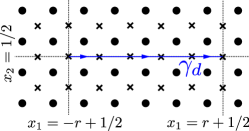
Figure 3.

with $\ell\geq d$. (one could think that $\ell\gg d$ is necessary but that does not make any difference for the upcoming result) For the rest, $v$ is arbitrary but such that $\left\|\mathrm{d}v\right\|\leq C$. The operator implementing this potential is $V=\langle v,n\rangle$ and so we have specified both $J=J_{\gamma_{d}}$ and $V$, see Figure 4(a).

Lemma 4.2.

With $V,J$ chosen as in the lines above, we have

(4.3) $$\left|\kappa-\frac{\chi_{J,V}}{2Ed}\right|={\mathcal{O}}(1/d).$$

The relatively large error ${\mathcal{O}}(1/d)$ in this theorem is explained by realizing that the current operator $J_{\gamma_{d}}$ itself is only defined unambiguously up to terms of norm unity at the edges of the line segment, see Section 2.4. This also shows the way to a solution: We note that (4.1) also equals $\frac{\langle J_{\gamma_{d}}\rangle}{\Delta v}$ with $\Delta v$ the change in potential along the line segment (in other words: for transverse conductivity in 2D, conductivity equals conductance). One is tempted to modify the setup so that the endpoints of $\gamma_{d}$ are in a field-free region. Here is a possible way: We keep the electric field the same as before in the strip $\{|x_{1}|\leq\ell\}^{e}$ and we insist that it is identically zero in the strips $\{\ell<|x_{1}|<\ell+2r\}^{e}$ with $r\gg 1$. The length $2d$ of path $\gamma_{d}$ is now chosen $d=\ell+r$, see Figure 4(b). So, to nail down the model precisely, we take $J=J_{\gamma_{d}}$ (defined above Lemma 4.2) with $d=\ell+r$ and $V=\langle v,n\rangle$ with

(4.4) $${\mathrm{d}}v=\begin{cases}E\mathrm{d}x_{1}&\text{on}\quad\{|x_{1}|\leq\ell\}^{e}\\ 0&\text{on}\quad\{\ell<|x_{1}|\leq\ell+2r\}^{e}\end{cases}$$

and $v$ arbitrary elsewhere but with $\left\|\mathrm{d}v\right\|\leq C$. We write $\Delta v=v(\ell,0)-v(-\ell,0)$

Theorem 4.3.

With $V,J$ chosen as in the lines above

(4.5) $$\left|\kappa-\frac{\chi_{J,V}}{\Delta v}\right|={\mathcal{O}}\big{(}r^{-\infty}\big{)}.$$

As anticipated, the above result has a much better accuracy than Lemma 4.2. What is however not yet explicitly exhibited, is the topological nature of the response coefficient. We still have a relevant region of constant electric field. However, we note that the error term only depends on $r$ and not on $\ell,d$ separately: the entire potential difference can also be realized along a single site spacing ($\ell=1$). This already shows that it is not important to have a region around where the electric field is well-defined. We can take this a step further and cast the result in a much more robust way. Let us deform the path $\gamma$, allowing it to be an arbitrary path in $\Gamma^{*}$ that is part of the oriented boundary of some set (cf. (2.5)). We denote the begin-and endpoints of $\gamma$ by $y_{\rm b},y_{\rm e}\in\Gamma^{*}$, thus also specifying an orientation for $\gamma$. We now consider a potential $v$ that is flat on spheres of radius $r$ around $y_{\rm b}$ and $y_{\rm e}$, see Figure 4(c). Abusing the notation slightly, we denote by $v(y_{\rm b}),v(y_{\rm e})$ the two values that $v$ takes in the vicinity of $v(y_{\rm b}),v(y_{\rm e})$. We then define the potential difference $\Delta v=v(y_{\rm e})-v(y_{\rm b})$. We set $J=J_{\gamma}$, then

Lemma 4.4.

With $V,J$ chosen as in the lines above

(4.6) $$\left|\kappa-\frac{\chi_{J,V}}{\Delta v}\right|={\mathcal{O}}\big{(}r^{-\infty}\big{)}.$$

This lemma is our most revealing result on the Kubo response.

(a) Setup for Lemma 4.2. The current is measured across a small segment in the bulk of the electric field. As indicated, since the field $\mathrm{d}v$ is derived from a potential, it must be non-zero somewhere outside the region $\{\lvert x_{1}\rvert\leq l\}$ as well.

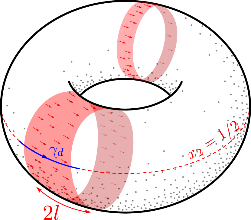
(b) Setup for Theorem 4.3. The current is measured across a line that completely traverses the region of electric field.

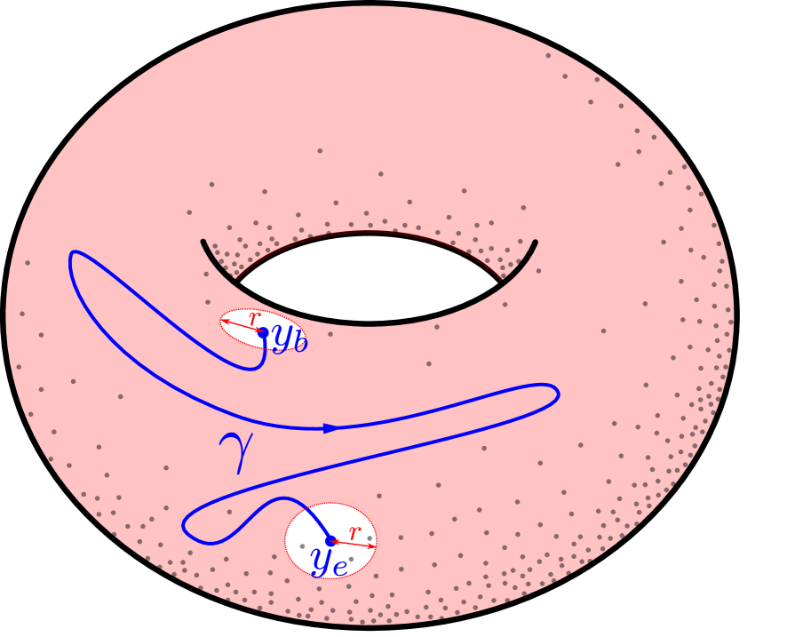
(c) Setup for Lemma 4.4. The electric field $\mathrm{d}v$ is nonzero only in the red region.

4.2. From Kubo response to adiabatic response

The setup of adiabatic response demands that we specify a slow change in the Hamiltonian. In the context of Hall fluids, the natural change is to slowly thread a flux. Hence, we take up the setup introduced in Section 2.3, we choose a vortex free vector potential $A$ and define

$$H_{s}:=H_{sA}$$

As we saw in Section 3.2 a special role is played by the derivative $W:=\partial_{s}H_{s}\big{|}_{s=0}$. In our case, this derivative is locally computed to be

(4.7) $$(W)_{\Sigma}=\mathrm{i}\>([\langle\theta,n\rangle,H]))_{\Sigma}$$

where $\Sigma$ is a region in which $A$ is exact, i.e. $A=\mathrm{d}\theta$ on $\Sigma^{e}$, see Section 2.3. The commutator in the right-hand side of the previous formula reminds us of the frequency derivative linking the adiabatic and Kubo responses. If $J$ has support in the far interior of $\Sigma$, we can pretend that (4.7) holds globally, leading to

Theorem 4.5.

Let $J$ be supported in $X$, such that $\mathrm{dist}(X,\Gamma\setminus\Sigma)\geq r$, with $A=\mathrm{d}\theta$ on $\Sigma^{e}$. Then

$$\left|\chi^{\mathrm{ad}}_{J,H_{s}}-\chi_{J,V}\right|={\mathcal{O}}(r^{-\infty}),\qquad\text{with}\quad V=\langle\theta,n\rangle.$$

The above theorem tells us that adiabatically switching on a vector potential evokes the same response as driving with an electric field (derived from the electrostatic potential $\theta$). This is demystified by recalling the standard electrodynamics relation $E={\mathrm{d}}v-\partial_{t}A$ and noting that we have here an $A$ that is linear in the rescaled time $s=\epsilon t$, and the observable $J$ allows to restrict to a region where $A={\mathrm{d}}\theta$. Hence $E=-{\mathrm{d}}\theta$ and $\theta$ plays the role of an electrostatic potential $v$. This is precisely the content of the above theorem.

To belabour this point, we provide a corollary to Theorem 4.5 that applies to a Hall setup. Consider a path $\gamma$ that has the regularity also required in Lemma 4.4 ( i.e. $\gamma$ is part of the boundary of some set) but we allow for the path to be closed as well. We consider a vortex-free vector potential $A$ that vanishes in the balls of radius $r$ around the points $y_{b}$ and $y_{e}$ (for closed paths, there is no requirement, and then we formally take $r={\mathcal{O}}(L)$). Define ${\mathcal{E}}:=\int_{\gamma}A$ (the suggestion is that this is an emf, ie. electromotive force)

Corollary 4.6.

Let $H_{s}=H_{sA}$ with $A$, $J=J_{\gamma}$ and ${\mathcal{E}}$ as described above, then we have

$$\left|\kappa-\frac{\chi^{\mathrm{ad}}_{J,H_{s}}}{{\mathcal{E}}}\right|={\mathcal{O}}(r^{-\infty}).$$

In the case of an open path, this corollary is an immediate consequence of Theorem 4.5 and Lemma 4.4, as one can always choose a gauge $\theta$ locally so that $A=\mathrm{d}\theta$. For closed paths, this might be impossible. In that case one can for example follow the steps of the proof of Thoerem 4.3, or, alternatively, still use Theorem 4.5 for several paths glued together in regions of diameter $cL$ where $\mathrm{d}A$ vanishes.

5. Proofs

5.1. Preliminaries

Let $W\in L^{\infty}({\mathbb{R}})\cap L^{1}({\mathbb{R}})$ be an odd function such that

1. $\left|W(t)\right|={\mathcal{O}}(|t|^{-\infty})$

2. $\widehat{W}(\zeta)=\frac{-\mathrm{i}}{\sqrt{2\pi}\zeta},\quad\text{if }\lvert\zeta\rvert\geq g/2.$

where $\widehat{W}$ is the Fourier transform of $W$. See [15, 16] for a construction of such $W$. Then we define the map ${\mathcal{I}}$ (acting on operators $O$)

(5.1) $${\mathcal{I}}(O)={\mathcal{I}}_{H}(O):=\int_{-\infty}^{\infty}\mathrm{d}t\;W(t)\mathrm{e}^{\mathrm{i}tH}O\mathrm{e}^{-\mathrm{i}tH}.$$

Furthermore, we need the off-diagonal projection

$$O\mapsto\bar{O}=POP^{\perp}+P^{\perp}OP,\qquad P^{\perp}=1-P$$

where we recall that $P$ is the (one-dimensional) ground state projection of $H$. We summarize the useful properties of these objects.

Lemma 5.1.

Let $O,O^{\prime}$ be arbitrary operators. We write $\mathrm{ad}_{H}(O)=[H,O]$.

1. $\omega(OO^{\prime})=\omega(\bar{O}O^{\prime})=\omega({O}\bar{O^{\prime}})=\omega(\bar{O}\bar{O^{\prime}})$.

2. $\overline{{\mathcal{I}}(O)}={{\mathcal{I}}(\bar{O})}$.

3. $\mathrm{ad}_{H}\,{\mathcal{I}}(\bar{O})=\mathrm{i}\bar{O}$.

4. ${\mathcal{I}}\,\mathrm{ad}_{H}(\bar{O})=\mathrm{i}\bar{O}$.

5. If $O$ has support in $S$ then $\left\|{\mathcal{I}}(O)-({\mathcal{I}}(O))_{S^{r}}\right\|=\left\|O\right\|\lvert S\rvert\times{\mathcal{O}}(r^{-\infty})$.

6. $\left\|{\mathcal{I}}(O)\right\|\leq\left\|W\right\|_{1}\left\|O\right\|$.

Proof.

We view the algebra of operators as a Hilbert space with the Hilbert Schmidt scalar product (remember that all is finite-dimensional). This makes $\mathrm{ad}_{H}$ into a Hermitian operator and we define $\widehat{W}(\mathrm{ad}_{H})$ by spectral calculus. From (5.1), we see that ${\mathcal{I}}=\sqrt{2\pi}\widehat{W}(\mathrm{ad}_{H})$. This proves that ${\mathcal{I}}$ and $-\mathrm{i}\mathrm{ad}_{H}$ are inverses on the spectral subspace $|\mathrm{ad}_{H}|\geq g/2$. By the gap assumption, this subspace contains all $\bar{O}$. Hence $(iii),(iv)$ are shown. The claim $(v)$ follows by the Lieb-Robinson bound and the remaining claims are obvious. ∎

Lemma 5.2.

Consider vector potentials $A=A(\phi_{1},\phi_{2})$ threading fluxes $(\phi_{1},\phi_{2})$ as defined in Section 3.3. Then

$$K_{j}={\mathcal{I}}(\partial_{\phi_{j}}H_{A}),\qquad j=1,2$$

(with derivatives taken at $\phi=0$) are generators of parallel transport, i.e. they satisfy (3.9).

For the proofs, see [15, 16] for the case of spin systems and [17, 18, 19] for fermionic systems.

Lemma 5.3.

Let $G,G^{\prime}$ be local Hamiltonians in the sense of Section 2.1. Let $Z$ be the intersection of their supports. Then

$$[{\mathcal{I}}(G),{\mathcal{I}}(G^{\prime})]=[{\mathcal{I}}(G_{Z^{r}}),{\mathcal{I}}(G^{\prime}_{Z^{r}})]+{\mathcal{O}}(r^{-\infty}),\qquad[{\mathcal{I}}(G),G^{\prime}]=[{\mathcal{I}}(G_{Z^{r}}),G^{\prime}_{Z^{r}}]+{\mathcal{O}}(r^{-\infty})$$

Proof.

We split the local Hamiltonians in local terms and use Lemma 5.1 (v) and (vi). ∎

5.2. Proof of Lemma 3.1: Thermodynamic limit

Let us denote the quantity in (3.2) without limits as

$$\chi(\epsilon,L):=\mathrm{i}\>\int_{0}^{\infty}\mathrm{d}t\;\omega\left([V(-t),J]\right)\mathrm{e}^{\mathrm{i}\nu t-\epsilon t},$$

dropping hence $V,J,\nu$ from the notation. We keep in mind that $J,V$ are independent of $L$ (see Section 2.1). We now proceed in three steps.

Lemma 5.4.

For any $\epsilon>0$, the following exists

$$\chi(\epsilon,\infty):=\lim_{L\to\infty}\chi(\epsilon,L)$$

Proof.

Indeed, for any finite $t$, the $\lim_{L}\omega\left([V(-t),J]\right)$ exists by Assumption 2.2 and locality of dynamics (Lieb-Robinson bound), and it is bounded by $\left\|V\right\|\left\|J\right\|$. Consequently, the limit of the $t$-integral exists by dominated convergence. ∎

We now state a lemma that expresses the main point, in the sense that one should not expect it to be true if the system were not gapped.

Lemma 5.5.

The limit $\chi(L)=\lim_{\epsilon\downarrow 0}\chi(\epsilon,L)$ exists and (for some $L$-independent $C$)

$$|\chi(\epsilon,L)-\chi(L)|\leq C\epsilon,\qquad\text{for $\epsilon\leq g$}$$

Proof.

Computing

$$\int_{0}^{\infty}\mathrm{d}t\;\overline{V}(-t)\mathrm{e}^{\mathrm{i}\nu t-\epsilon t}=-\mathrm{i}\;\left(\frac{1}{-(H+\nu)-\mathrm{i}\epsilon}P^{\perp}VP+PVP^{\perp}\frac{1}{(H-\nu)-\mathrm{i}\epsilon}\right)$$

and using Lemma 5.1 (i) we find

$$\chi(\epsilon,L)=\omega\left(VP^{\perp}\frac{1}{(H-\nu)-\mathrm{i}\epsilon}P^{\perp}J\right)-\omega\left(JP^{\perp}\frac{1}{-(H+\nu)-\mathrm{i}\epsilon}P^{\perp}V\right).$$

Since $\nu$ is smaller than $g/2$, half the gap of $H$, the limit is obviously the same expression with $\epsilon=0$ and the difference from the limit is, by functional calculus, bounded by ($\pm\nu$ corresponding to the two terms above)

$$2\left\|V\right\|\left\|J\right\|||{P^{\perp}}\frac{\epsilon}{(H\pm\nu)(H\pm\nu-\mathrm{i}\epsilon)}{P^{\perp}}||\,\leq\,\frac{C\epsilon}{g}(1+\frac{4\epsilon^{2}}{{g}^{2}})\left\|V\right\|\left\|J\right\|.$$

∎

Lemma 5.6.

The limit $\lim_{L\to\infty}\chi(L)$ exists.

Proof.

We use the language of Section 5.1, in particular we consider the operator $\mathrm{ad}_{H}$ acting on a Hilbert space. Since the spectrum of $\mathrm{ad}_{H}+\nu$ contains no points other than zero that are smaller than $g/2$ (remember that $\lvert\nu\rvert\leq g/2$), we find that

$$\chi(L)=\mathrm{i}\,\int\mathrm{d}t\;W(t)\;\mathrm{e}^{\mathrm{i}t\nu}\omega([{V}(-t),J]).$$

with the function $W$ defined in Section 5.1. The operator $\int\mathrm{d}t\;W(t)\;\mathrm{e}^{\mathrm{i}t\nu}{V}(-t)$ can be well-approximated by local operators, by the same reasoning as in the proof of Lemma 5.1 ($v$). The claim consequently follows by Assumption 2.2 and dominated convergence. ∎

Lemma 3.1 now follows directly by combining Lemmata 5.4, 5.5 and 5.6.

5.3. Proof of Lemma 3.2

In the course of the proof in Section 5.2, we have in particular obtained

(5.2) $$\chi_{J,V}=\mathrm{i}\,\omega([{\mathcal{I}}(V),J]).$$

The locality now follows directly from Lemma 5.3.

5.4. Proof of Lemma 3.3

Starting from (3.4), it was shown in [13] that

$$\chi^{\mathrm{ad}}_{J,H}=\mathrm{i}\,\omega([{\mathcal{I}}(K),J]),\qquad K=K_{s=0}.$$

We now connect RHS of (3.6), lets call it $\chi$, to this expression. Lemma 5.1 says that the operation ${\mathcal{I}}$ is an inverse of $-i\mathrm{ad}_{H}$ when restricted to an appropriate space. In particular using points (i) and (iv) of the lemma we get that

$$\omega([{\mathcal{I}}(O(-t)),O^{\prime}])$$

is a primitive function of $\omega([O(-t),O^{\prime}])$ for any observables $O,O^{\prime}$. Integrating the expression (3.6) for $\chi$ by parts we obtained

$$\chi=-\mathrm{i}\lim_{\epsilon\to 0^{+}}\int_{0}^{\infty}\mathrm{d}t\;(1-\epsilon)\mathrm{e}^{-\epsilon t}\omega\left([{\mathcal{I}}(W(-t)),J]\right).$$

By the same arguments that were used to prove the existence of thermodynamic limit, the part with $\epsilon$ vanishes in the limit. Noting that ${\mathcal{I}}(W)=K$ and integrating by parts again we get

$$\chi=\mathrm{i}\lim_{\epsilon\to 0^{+}}\omega\left([{\mathcal{I}}(K),J]\right)-\mathrm{i}\lim_{\epsilon\to 0^{+}}\int_{0}^{\infty}\mathrm{d}t\;\epsilon\,\mathrm{e}^{-\epsilon t}\omega\left([{\mathcal{I}}(K(-t)),J]\right).$$

The second part again vanishes in the limit and we obtain $\chi=\chi^{\mathrm{ad}}_{J,H}$.

5.5. Proof of Lemma 3.4

From  (2.3) we see that the projections $P^{\prime}(\phi)$ are related to $P(\phi)$ through the gauge transformation $U(\phi)=\mathrm{e}^{\mathrm{i}\langle\phi_{1}\theta_{1}+\phi_{2}\theta_{2},n\rangle}$, therefore

$$\partial_{1,2}P^{\prime}(\phi)=U(\phi)\big{(}\mathrm{i}[\langle\theta_{1,2},n\rangle,P(\phi)]+\partial_{1,2}P(\phi)\big{)}U(\phi)^{*}.$$

Let’s write ${V}_{1,2}=\langle\theta_{1,2},n\rangle$, then the adabatic curvature for the family of projections $P^{\prime}(\phi)$ is (all derivatives at $\phi=0$)

$$\mathrm{i}\;\omega^{\prime}\left([\partial_{1}P^{\prime},\partial_{2}P^{\prime}]\right) =\mathrm{i}\;\omega\left([\partial_{1}P,\partial_{2}P]\right)$$

$$-\omega\left([[{V}_{1},P],\partial_{2}P]\right)$$

$$-\omega\left([\partial_{1}P,[{V}_{2},P]]\right)$$

$$-\mathrm{i}\;\omega\left([[{V}_{1},P],[{V}_{2},P]]\right).$$

The first term on the right-hand side is the adiabatic curvature $\kappa$ of the family $P(\phi)$, it remains to show that the other three terms vanish. The fourth term is $\mathrm{i}\,\omega\left([{V}_{1},{V}_{2}]\right)=0$ by the same algebra as in (3.10), because $[{V}_{1},{V}_{2}]=0$. We show now why the second term vanishes up to ${\mathcal{O}}(L^{-\infty})$ (the third term is analogous). We have

(5.3) $$\omega\left([[{V}_{1},P],\partial_{2}P]\right)=\mathrm{i}\;\omega\left([{V}_{1},{\mathcal{I}}\big{(}\partial_{2}H_{A}\big{)}]\right)=\mathrm{i}\sum_{x}\theta_{1}(x)\;\omega\left([n_{x},{\mathcal{I}}\big{(}\partial_{2}H_{A}\big{)}]\right).$$

For each $x$, we consider a region $\Sigma^{x}$ of diameter ${\mathcal{O}}(L)$ centered on $x$. In this region, we have $A=d(\phi_{1}f_{1}+\phi_{2}f_{2})$ for some $f_{1,2}$ and hence

$$(\partial_{2}H_{A}\big{)}_{\Sigma^{x}}=([\langle f_{2},n\rangle,H\big{)}_{\Sigma^{x}}.$$

In the last expression, we changed $H_{A}\to H$ as the derivative was at $\phi=0$. Because of locality of ${\mathcal{I}}$ and the boundedness of $A$, we have

$$[n_{x},{\mathcal{I}}\big{(}\partial_{2}H\big{)}]=[n_{x},{\mathcal{I}}\big{(}[\langle f_{2},n\rangle,H]\big{)}]+{\mathcal{O}}(L^{-\infty}).$$

Now,

$$\omega\left([n_{x},{\mathcal{I}}\big{(}[\langle f_{2},n\rangle,H]\big{)}]\right)=\omega\left([n_{x},{{\langle f_{2},n\rangle}}]\right)=0$$

where we used Lemma 5.1 (i), (ii) and (iv). The claim is proven by plugging this into (5.3).

5.6. Proof of Theorem 4.3

We start from

(5.4) $$\chi=\mathrm{i}\,\omega([{\mathcal{I}}(\bar{V}),J]),$$

Because the function $W$ in the definition of ${\mathcal{I}}$ is odd, we have also

(5.5) $$\chi=-\mathrm{i}\,\omega([\bar{V},{\mathcal{I}}(J)]).$$

Using Lemma 5.1 (iv), we then obtain

(5.6) $$\chi=-\omega([{\mathcal{I}}([H,\bar{V}]),{\mathcal{I}}(J)])=-\omega([{\mathcal{I}}([H,V]),{\mathcal{I}}(J)])$$

The intersection of the supports of $[H,V]$ and $J$ is contained in

$$Z:=\{|x_{1}|\leq\ell+C,|x_{2}|\leq C\},$$

see Figure 5. Since $[H,V]$ and $J$ are clearly ‘local Hamiltonians’, we can apply Lemma 5.3 to conclude that (5.6) equals

(5.7) $$[{\mathcal{I}}([H,V]),{\mathcal{I}}(J)]=[{\mathcal{I}}([H,V]_{Z^{r}}),{\mathcal{I}}(J_{Z^{r}})]+{\mathcal{O}}(r^{-\infty}).$$

Now, let us approach from a different angle and consider the vector potential

$$A=\phi_{1}A_{1}+\phi_{2}A_{2}$$

where

1. $A_{1}=dv$ on $\{|x_{1}|\leq\ell+2r\}^{e}$ and $A_{1}=0$ elsewhere. Here $v$ was defined just above Theorem 4.3.

2. $A_{2}=dh_{2}$ on $\{|x_{2}\leq C|\}^{e}$ and $A_{2}=0$ elsewhere, with $h_{2}$ the Heaviside function $h_{2}(x)=1(x_{2}>0)$.

The most relevant properties of $A$ are that

(5.8) $$[H,V]_{Z^{r}}=\mathrm{i}(\partial_{\phi_{1}}H_{A})_{Z^{r}},\qquad J_{Z^{r}}=(\partial_{\phi_{2}}H_{A})_{Z^{r}}$$

see (2.4) and (2.5). Additionally, the intersection of the supports of $\partial_{1}H_{A}$ and $\partial_{2}H_{A}$ (derivatives at $\phi=0$ is also contained in $Z$ and these are also local Hamiltonians, so Lemma 5.3 applies here as well. Combining this fact with (5.7) and (5.8), we conclude that

$$[{\mathcal{I}}([H,V]),{\mathcal{I}}(J)]=\mathrm{i}[{\mathcal{I}}((\partial_{\phi_{2}}H_{A})),{\mathcal{I}}((\partial_{\phi_{1}}H_{A}))]+{\mathcal{O}}(r^{-\infty})$$

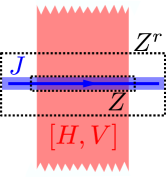
Figure 5. The supports of $[H,V]$ and $J$, and the sets $Z$ and $Z^{r}$ in a neighbourhood of the location where the current is measured.

The expression on the right is almost of the type as appeared in the definition of adiabatic curvature, except that there we demanded that $A$ threads fluxes $\phi_{1},\phi_{2}$. In our situation, $\phi_{1}A_{1}$ threads a flux $\phi$, but $\phi_{2}A_{2}$ threads a flux $2\phi_{2}\ell E=\phi_{2}\Delta v$. This shows that the $\omega(\cdot)$ of the above commutator is given by $(\Delta v)\kappa$ instead of $\kappa$. This proves Theorem 4.3.

5.7. Proof of Lemma 4.4

The same as above, but with different vector potentials $A_{1}^{\prime},A_{2}^{\prime}$ that are however related to $A_{1},A_{2}$ by gauge transformations.

5.8. Proof of Lemma 4.2

Lemma 4.2 uses $\ell$ and $d\leq\ell$. We prove the lemma for $d=\ell$. This suffices because, if $d<\ell$ then we modify the potential $v$ by making it flat for $|x_{1}|\geq d$. By the locality estimate 3.2, this changes the response coefficient by ${\mathcal{O}}(1)$, which is compatible with the claim of the lemma. Now to the argument for $d=\ell$. Theorem 4.3 applies to our situation, with the modification that the path $\gamma$ in $J_{\gamma}$ has length $2(\ell+r)$, whereas we need a shortened path $\gamma^{\prime}$ of length $2\ell$. However, $J_{\gamma^{\prime}}=J_{\gamma}+{\mathcal{O}}(r)$ and this difference gives a contribution of order ${\mathcal{O}}(r)$ in the response coefficient. This follows indeed from the representation in 3.2 and the bound in Lemma 5.1(vi). Upon division by $\ell$ we get the desired claim.

5.9. Proof of Theorem 4.5

We start from the expression (Section 5.4)

$$\chi^{\mathrm{ad}}_{J,H}=\mathrm{i}\,\omega([{\mathcal{I}}(K),J]),\qquad K=K_{s=0}.$$

By Lemma 5.2 and the definition of $W$, we have $K={\mathcal{I}}(\partial_{s}H_{s}|_{s=0})={\mathcal{I}}(W)$, so that

$$\chi^{\mathrm{ad}}_{J,H}=\mathrm{i}\,\omega([{\mathcal{I}}({\mathcal{I}}(W)),J])=-\mathrm{i}\,\omega([{\mathcal{I}}(W),{\mathcal{I}}(J)])$$

From (4.7), we know that $W_{\Sigma}=\mathrm{i}[V,H]_{\Sigma}$. Since the observable $J$ is supported far from $\Lambda\setminus\Sigma$, we invoke Lemma 5.3 to get

$$\chi^{\mathrm{ad}}_{J,H}=\omega([{\mathcal{I}}([V,H]),{\mathcal{I}}(J)])+{\mathcal{O}}(r^{-\infty})$$

By Lemma 5.1 $(i),(ii),(iv)$, the right-hand side equals $-\mathrm{i}\,\omega([V,{\mathcal{I}}(J)])=\mathrm{i}\,\omega([{\mathcal{I}}(V),J])$, which was to be proven.

6. Appendix

We provide the necessary definitions for the framework of discrete one-forms $A$ on $\Gamma$.

6.1. The vector field of one-forms

Let $\Gamma^{e}:=\{(x,y)\in\Gamma^{2}\;:\;x\sim y\}$ be the set of oriented edges of $\Gamma$. For any oriented edge $(x,y)$, let $\overline{(x,y)}=(y,x)$ be the reversed edge. A one-form is a function $A:\Gamma^{e}\rightarrow{\mathbb{R}}$ such that $A(e)=-A(\overline{e})$.

6.2. Integration of one-forms along paths

For an oriented edge $(x,y)$ we define $i((x,y))=x$ and $f((x,y))=y$. An oriented path in $\Gamma$ is an ordered set of oriented edges $\gamma=(e_{1},\cdots,e_{N})$ such that $f(e_{i})=i(e_{i+1})$ for $i=1,\cdots N-1$. The integral of the one-form $A$ along the oriented path $\gamma$ is defined by

(6.1) $$\int_{\gamma}A:=\sum_{e\in\gamma}A(e).$$

6.3. Contractible loops and vortex free one-forms

For any path $\gamma=(e_{1},\cdots,e_{N})$ we write $i(\gamma)=i(e_{1})$ for the startingpoint and $f(\gamma)=f(e_{N})$ for the endpoint of the path. A loop is a path $\gamma$ for which $i(\gamma)=f(\gamma)$. We wish to classify loops as ‘contractible’ or ‘non-contractible’ in such a way that we recover the usual homology of the two-torus.

One way of doing this is to think of the discrete torus $\Gamma$ as a subset of a smooth flat torus ${\mathbb{T}}^{2}$. We associate to each edge $(x,y)$ of $\Gamma$ a curve tracing the shortest path from $x$ to $y$ in the torus ${\mathbb{T}}^{2}$. To each path $\gamma$ we associate the curve obtained by concatenating the curves associated to the edges of $\gamma$. I this way, a closed curve in ${\mathbb{T}}^{2}$ is associated to each loop in $\Gamma$. We say that the loop $\gamma$ is contractible if its associated curve is contractible in ${\mathbb{T}}^{2}$.

A one-form $A$ is exact in the region $\Sigma\subset\Gamma$ if $\oint_{\gamma}A=0$ whenever $\gamma$ is a contractible loop in $\Sigma$.

Let $\theta:\Gamma\rightarrow{\mathbb{R}}$, then we define its exterior derivative to be

(6.2) $$\mathrm{d}\theta\big{(}(x,y)\big{)}=\theta(y)-\theta(x).$$

$\mathrm{d}\theta$ is exact in any subset of $\Gamma$, the integral of $\mathrm{d}\theta$ vanishes along all loops, even the non-contractible ones.

Conversely, if $A$ is exact in the region $\Sigma$, then there exist a function $\theta:\Sigma\rightarrow{\mathbb{R}}$ such that $A\big{|}_{\Sigma^{e}}=\mathrm{d}\theta$. Indeed, pick a point $x_{0}$ in each connected component of $\Sigma$ and put $\theta(x_{0})=0$. For any other point $x$ that is path-connected to $x_{0}$, take any path $\gamma$ from $x_{0}$ to $x$ that lies in $\Sigma$ and define $\theta(x)=\int_{\gamma}A$. This definition is independent of the chosen path because $A$ is exact in $\Sigma$. Now, for any edge $(x,y)\in\Sigma^{e}$ we have

$$\mathrm{d}\theta\big{(}(x,y)\big{)}=\theta(y)-\theta(x)=\int_{\gamma_{y}}A-\int_{\gamma_{x}}A=\int_{\{(x,y)\}}A=A\big{(}(x,y)\big{)}$$

where $\gamma_{x}$ and $\gamma_{y}$ are paths in $\Sigma$ from $x_{0}$ to $x$ and to $y$ respectively.

References

- [1] Q. Niu, D.J. Thouless, and Y.-S. Wu. Quantized Hall conductance as a topological invariant. Phys. Rev. B, 31(6):3372, 1985.
- [2] J.E. Avron and R. Seiler. Quantization of the Hall conductance for general, multiparticle Schrödinger Hamiltonians. Phys. Rev. Lett., 54(4):259–262, 1985.
- [3] M.B. Hastings and S. Michalakis. Quantization of Hall conductance for interacting electrons on a torus. Commun. Math. Phys., 334:433–471, 2015.
- [4] Jean-Bernard Bru and Walter de Siqueira Pedra. Microscopic conductivity of lattice fermions at equilibrium. part ii: Interacting particles. Letters in Mathematical Physics, 106(1):81–107, 2016.
- [5] A. Giuliani, V. Mastropietro, and M. Porta. Universality of the Hall conductivity in interacting electron systems. Commun. Math. Phys., 2016.
- [6] Sven Bachmann, Wojciech De Roeck, and Martin Fraas. The adiabatic theorem and linear response theory for extended quantum systems. Communications in Mathematical Physics, pages 1–31, 2018.
- [7] Sven Bachmann, Alex Bols, Wojciech De Roeck, and Martin Fraas. Quantization of conductance in gapped interacting systems. 19(3):695–708, 2018.
- [8] Barry Simon. The statistical mechanics of lattice gases, volume 1. Princeton University Press, 2014.
- [9] D.R. Hofstadter. Energy levels and wave functions of Bloch electrons in rational and irrational magnetic fields. Phys. Rev. B, 14(6):2239–2249, 1976.
- [10] MB Hastings. The stability of free fermi hamiltonians. arXiv preprint arXiv:1706.02270, 2017.
- [11] Wojciech De Roeck and Manfred Salmhofer. Persistence of exponential decay and spectral gaps for interacting fermions. Communications in Mathematical Physics, Jul 2018.
- [12] R. Kubo. Statistical-mechanical theory of irreversible processes. I. General theory and simple applications to magnetic and conduction problems. J. Phys. Soc. Japan, 12(6):570–586, 1957.
- [13] Sven Bachmann, Wojciech De Roeck, and Martin Fraas. Adiabatic theorem for quantum spin systems. Physical review letters, 119(6):060201, 2017.
- [14] Sven Bachmann, Alex Bols, Wojciech De Roeck, and Martin Fraas. A many-body index for quantum charge transport. arXiv preprint arXiv:1810.07351, 2018.
- [15] M.B. Hastings and X.-G. Wen. Quasiadiabatic continuation of quantum states: The stability of topological ground-state degeneracy and emergent gauge invariance. Phys. Rev. B, 72(4):045141, 2005.
- [16] S. Bachmann, S. Michalakis, S. Nachtergaele, and R. Sims. Automorphic equivalence within gapped phases of quantum lattice systems. Commun. Math. Phys., 309(3):835–871, 2012.
- [17] J-B Bru and Walter de Siqueira Pedra. Lieb-Robinson bounds for multi-commutators and applications to response theory, volume 13. Springer, 2016.
- [18] D. Monaco and S. Teufel. Adiabatic currents for interacting electrons on a lattice. arXiv preprint arXiv:1707.01852, 2017.
- [19] B. Nachtergaele, R. Sims, and A. Young. Stability of gapped phases of fermionic lattice systems. In preparation.