Abstract

The Leptoquark model has been instrumental in explaining the observed lepton flavour universality violating charged ($b\to c$) and neutral ($b\to s$) current anomalies that have been the cause for substantial excitement in particle physics recently. In this article we have studied the role of one (designated as $V_{2}^{\frac{4}{3}}$) of the components of ${V}_{2}$ Vector Leptoquark doublet with electromagnetic charge $\frac{4}{3}$ in explaining the neutral current ($b\to s$) anomalies $R_{K^{(*)}}$ and $B_{s}\to\mu^{+}\mu^{-}$. Moreover, we have performed a thorough collider search for this $V_{2}^{\frac{4}{3}}$ Leptoquark using $b\bar{b}\ell^{+}\ell^{-}$ ($\ell\equiv e,\mu$) final state at the Large Hadron Collider. From our collider analysis we maximally exclude the mass of the $V_{2}^{\frac{4}{3}}$ Leptoquark up to 2340 GeV at 95% confidence level for the 13 TeV Large Hadron Collider for an integrated luminosity of 3000 ${\rm fb}^{-1}$. Furthermore, a significant portion of the allowed parameter space that is consistent with the neutral current ($b\to s$) observables is excluded by collider analysis.

1 Introduction

The discovery of the Higgs boson in 2012 by the CMS [1] and ATLAS [2] collaborations is definitely one of the greatest achievements of Large Hadron Collider (LHC). Unfortunately, it has not been able to detect signatures corresponding to any new physics (NP) particles till date. On the other hand experimental measurements of observables related to $B$ physics have, however, exhibited deviations of a few $\sigma$ from their Standard Model (SM) expectations hinting towards the existence of beyond SM (BSM) physics. $B$-physics experiments at LHCb, Belle and Babar have pointed at intriguing lepton flavour universality violating (LFUV) effects. To that end, flavour changing neutral current (FCNC) processes such as $b\to s\mu^{+}\mu^{-}$ have drawn much attention due to anomalies that have been observed recently at the LHCb and Belle experiments. A deviation of 2.6$\sigma$ has been observed in $R_{K}={\rm BR}(B^{+}\to K^{+}\mu^{+}\mu^{-})/{\rm BR}(B^{+}\to K^{+}e^{+}e^{-})$ with a value of $0.745^{+0.090}_{-0.074}\pm 0.036$ [5] from the corresponding SM prediction ($R_{K}\approx 1$ [6, 7]) for the integrated di-lepton invariant mass squared range $1<q^{2}<6$ ${\rm GeV}^{2}$. LHCb has reported a deviation in $R_{K^{*}}={\rm BR}(B^{0}\to K^{*0}\mu^{+}\mu^{-})/{\rm BR}(B^{0}\to K^{*0}e^{+}e^{-})$ at the level of $2.1-2.3\sigma$ and $2.4-2.5\sigma$ for the two $q^{2}$ ranges [0.045-1.1] (called low-bin) and [1.1-6.0] ${\rm GeV^{2}}$ (called central-bin) with values $0.660^{+0.110}_{-0.070}\pm 0.024$ [8] and $0.685^{+0.113}_{-0.069}\pm 0.047$ [8] respectively. The corresponding SM predictions are $0.92\pm 0.02$ [9] and $1.00\pm 0.01$ [6, 7] respectively.

In order to explain the above mentioned anomalies we have selected a particular extension of the SM consisting of several hypothetical particles that mediate interactions between quarks and leptons at tree-level. Hence, these particles are known as Leptoquarks (LQs). Such particles can appear naturally in several extensions of the SM (e.g., composite models [10], Grand Unified Theories [11, 12, 13, 14, 15, 16, 17, 18], superstring-inspired ${\rm E_{6}}$ models [19, 20, 21, 22] etc). Considerable amount of work regarding LQs have been done both from the point of view of their diverse phenomenological aspects [23, 24, 25], and specific properties [26, 27, 28, 29, 30, 31, 32, 33, 34, 35, 36, 37, 38, 39, 40, 41, 42, 43, 44, 45, 46, 47, 48, 49, 50, 51, 52, 53, 54, 55, 56]. Furthermore, several articles  [57, 58, 59, 60, 61, 62, 49, 63, 64, 65, 66, 67, 68, 69, 70, 71, 72, 73, 74] that explain the different flavour anomalies with different versions of LQ models exist in the literature.

In connection to the above, we consider one of the components of the ${V}_{2}$ vector leptoquark (VLQ) doublet (the $V_{2}^{\frac{4}{3}}$) that is capable of mediating the $b\to s$ observables at tree level, due to its electromagnetic charge $Q=\frac{4}{3}$. We provide bounds on the parameter space for the $V_{2}^{\frac{4}{3}}$ VLQ subject to constraints due to the observables $R_{K^{(*)}}$. Furthermore, we have used the latest experimental value $2.8^{+0.7}_{-0.6}\times 10^{-9}$ [75] of the branching fraction for the decay $B_{s}\to\mu^{+}\mu^{-}$ as another constraint in our analysis while the SM prediction for the same decay is $3.66\pm 0.23\times 10^{-9}$ [76]. Out of the eight Wilson coefficients (given in eq. 10 of sec. 3) that contribute to the above $b\to s$ observables mediated by the $V_{2}^{\frac{4}{3}}$ VLQ, only four are independent. This allows us to numerically solve for these coefficients and in turn provide constraints on the real and imaginary parts for the allowed values of the coupling products $(g_{L,R})_{b\ell}(g_{L,R})_{s\ell}$ with respect to the mass of the $V_{2}^{\frac{4}{3}}$ VLQ up to $1\sigma$ (corresponding to the $1\sigma$ experimental errors for these observables).

The LQs being potential candidates in explaining the flavour anomalies, it is only relevant that one investigates the production and decay signatures of these LQs at colliders. There exist several articles [34, 35, 36, 38, 41, 47, 77, 78] in the literature that have been dedicated to collider studies of LQs, but in most of the cases these studies have been performed on scalar LQs. The collider studies for vector LQs are limited in number [33, 38, 55, 79, 80]. Our current interest for this article being the $V^{\frac{4}{3}}_{2}$ VLQ, it is imperative that one probes this LQ at the current or future collider experiments. To the best of our knowledge, the present article is the first which deals with the collider prospects of the $V^{\frac{4}{3}}_{2}$ VLQ at the LHC. We study signatures corresponding to this VLQ for $b\bar{b}\ell^{+}\ell^{-}$ final states at the LHC with the centre of momentum (CM) energy $\sqrt{s}=13$ TeV. Although the ATLAS collaboration has also looked at the same final state [82] but they have searched for the R-parity violating scalar top partners at the 13 TeV LHC. Their exclusion limit, depending on the branching fractions of the scalar top to bottom and electron/muon, is set from 600 GeV to 1500 GeV. Using several interesting kinematic variables we maximize the signal event with respect to relevant SM backgrounds. From our collider analysis and depending on the SM bilinear couplings with $V^{\frac{4}{3}}_{2}$ VLQ we exclude the mass of this VLQ up to 2140 GeV and 2340 GeV for the two bench mark values of integrated luminosities 300 ${\rm fb}^{-1}$ and 3000 ${\rm fb}^{-1}$ respectively at the 95% confidence level (C.L.). At this point, we would like to mention that the other component ($V_{2}^{\frac{1}{3}}$) of the ${V}_{2}$ VLQ with electromagnetic charge $Q=\frac{1}{3}$ has not been considered in this analysis primarily because it is unable to mediate the $b\to s\ell^{+}\ell^{-}$ interactions. In addition, the parameter values taken in this analysis result in a small value of the branching ratio of $V_{2}^{\frac{1}{3}}$ VLQ to up type quarks and charged leptons or any final state. Hence the collider reach would be weak compared to the signal we have considered.

The paper is organised as follows. We briefly discuss the Lagrangian for the $V_{2}$ VLQ and set the notations in section 2. In section 3 we show the flavour analysis of $b\rightarrow s$ transition observables mediated by the $V^{\frac{4}{3}}_{2}$ VLQ. Section 4 is dedicated to the collider analysis for $V^{\frac{4}{3}}_{2}$ with $b\bar{b}\ell^{+}\ell^{-}$ final states. Finally, we discuss our results and conclude in section 5.

2 Effective Lagrangian of ${V_{2}}$ vector Leptoquark

LQs are special kinds of hypothetical particles that carry both lepton (L) and baryon (B) number. Consequently they couple to both leptons and quarks simultaneously. Furthermore, they possess colour charge and fractional electromagnetic charges. However, unlike the quarks they are either scalars or vectors bosons. For further discussions regarding all LQ scenarios, one can look into the review [83]. Due to the above distinguishable properties, these LQs have several phenomenological implications with respect to the other BSM particles. In general there are twelve LQs, among them six are scalars ($S_{3}$, $R_{2}$, $\tilde{R_{2}},\tilde{S_{1}},S_{1},\bar{S_{1}}$) and the rest ($U_{3}$, $V_{2}$, $\tilde{V_{2}},\tilde{U_{1}},U_{1},\bar{U_{1}}$) transform vectorially under Lorentz transformations. In the current article we are particularly interested on ${V_{2}}$ VLQ in order to explain the $b\to s$ anomalies. Under the SM gauge group ${\rm{SU(3)_{C}\times SU(2)_{L}\times U(1)_{Y}}}$ the ${V_{2}}$ VLQ transforms as $({\bf{\bar{3},2}},\frac{5}{6})$. The Lagrangian which describes the interaction for the ${V_{2}}$ VLQ with the SM fermion bilinear is given as [83]

$$\mathcal{L}^{\rm LQ}_{\boldsymbol{V_{2}}}=(g_{L})_{ij}\bar{d}_{iR}^{C}\gamma^{\mu}{\boldsymbol{V_{2}}}^{a}_{,\mu}\epsilon^{ab}L^{b}_{jL}+(g_{R})_{ij}\bar{Q}_{iL}^{C,a}\gamma^{\mu}\epsilon^{ab}{\boldsymbol{V_{2}}}^{b}_{,\mu}\ell_{jR}+{\rm h.c.},$$ (1)

with $a,b\equiv 1,2$. Here, $Q^{\sf T}_{L}\equiv(u~{}~{}~{}d)$ represents the left handed quark doublet, $L^{\sf T}_{L}\equiv(\nu_{\ell}~{}~{}~{}\ell)$ denotes for the left handed lepton doublet, $d_{R}$ stands for the right handed down type quark singlet and $\ell_{R}$ is the right handed charged lepton singlet. Left (right) handed gauge coupling constants are represented by $(g_{L(R)})_{ij}$ with the fermion generation indices $i,j\equiv 1,2,3$. To avoid the constraint due to the proton decay from ${V_{2}}$ VLQ, we set the corresponding ${V_{2}}$ couplings for di-quark interactions to zero. As the ${V_{2}}$ VLQ is transformed as doublet under ${\rm SU(2)_{L}}$ gauge group hence this ${V_{2}}$ VLQ multiplet contains two components $V_{2}^{\frac{4}{3}}$ and $V_{2}^{\frac{1}{3}}$ having electromagnetic charges $\frac{4}{3}$ and $\frac{1}{3}$ respectively. In the following we will focus only on the one component $V_{2}^{\frac{4}{3}}$ carrying electromagnetic charge $\frac{4}{3}$. From hereon, we will refer to the $V_{2}^{\frac{4}{3}}$ VLQ simply as $V_{2}$.

3 Flavour signatures

We closely follow ref. [84] in the following discussion about the operator basis relevant to $b\to s\ell^{+}\ell^{-}$ decays and the expressions for the observables. The effective dimension six Hamiltonian at the mass scale of the $b$ quark is written as [84, 85]

$$\mathcal{H}_{eff} = -\frac{4G_{F}}{\sqrt{2}}\lambda_{t}\bigg{[}\sum_{i=1}^{6}C_{i}O_{i}+\sum_{i=7,8,9,10,P,S}{}(C_{i}O_{i}+C_{i}^{\prime}(\mu)O_{i}^{\prime}(\mu))+C_{T}O_{T}+C_{T5}O_{T5}\bigg{]},$$ (2)

where $\lambda_{t}=V_{tb}V_{ts}^{*}$. The $V_{2}$ VLQ contributes to the following two-quark, two-lepton operators:

$$O_{9} = \frac{e^{2}}{g^{2}}(\bar{s}\gamma_{\mu}P_{L}b)(\bar{\ell}\gamma^{\mu}\ell)\;,~{}~{}O_{10}=\frac{e^{2}}{g^{2}}(\bar{s}\gamma_{\mu}P_{L}b)(\bar{\ell}\gamma^{\mu}\gamma_{5}\ell)\;,$$

$$O_{S} = \frac{e^{2}}{16\pi^{2}}(\bar{s}P_{R}b)(\bar{\ell}\ell)\;,~{}~{}O_{P}=\frac{e^{2}}{16\pi^{2}}(\bar{s}P_{R}b)(\bar{\ell}\gamma_{5}\ell)\;,$$ (3)

and their corresponding “primed” counterparts. The chiraly flipped “primed” operators are obtained by an $L\leftrightarrow R$ exchange in the above operators. Here $e=\sqrt{4\pi\alpha}$ represents the unit for electromagnetic charge, $g$ is the strong coupling constant and $P_{R,L}=(1\pm\gamma_{5})/2$. The four-quark operators $O_{1-6}$ and the radiative penguin operators $O_{7,8}$ are provided in ref. [86]. The decay amplitudes for the $B\to K^{*}\ell^{+}\ell^{-}$ transition in terms of the effective Wilson coefficients (WCs) evaluated at the scale $\mu=m_{b}$ are provided in [87].

The theoretical expression for the branching fraction corresponding to the $B_{s}\to\ell^{+}\ell^{-}$ decay reads [84]

$${\rm BR}(B_{s}\to\ell^{+}\ell^{-}) = \tau_{B_{s}}f_{B_{s}}^{2}m_{B_{s}}^{3}\frac{G_{F}^{2}|\lambda_{t}|^{2}\alpha^{2}}{(4\pi)^{3}}\beta_{\ell}(m_{B_{s}}^{2})\bigg{[}\frac{m_{B_{s}}^{2}}{m_{b}^{2}}|C_{S}-C_{S^{\prime}}|^{2}(1-\frac{4m_{\ell}^{2}}{m_{B_{s}}^{2}})+$$ (4)

$$|\frac{m_{B_{s}}}{m_{b}}(C_{P}-C_{P^{\prime}})+2\frac{m_{\ell}}{m_{B_{s}}}(C_{10}-C_{10}^{\prime})|^{2}\bigg{]}.$$

In the above $\beta_{\ell}=\sqrt{1-4m_{\ell}^{2}/q^{2}}$, $m_{B_{s}}$, $m_{b}$ and $m_{\ell}$ are denoted as the masses of $B_{s}$ meson, bottom quark ($b$) and charged lepton ($\ell$) respectively. $G_{F}$ is the Fermi constant, $\tau_{B_{s}}$ represents the life time while $f_{B_{s}}$ stands for the decay constant of $B_{s}$ meson. It is evident from eq. 4, that the ${\rm BR}(B_{s}\to\mu^{+}\mu^{-})$ (considering $\ell\equiv\mu$) is only sensitive to the contributions due to the differences between operators with left and right-handed quark currents, $C_{10}-C_{10}^{\prime}$, $C_{S}-C_{S}^{\prime}$ and $C_{P}-C_{P}^{\prime}$.

In contrast to the case for $B_{s}\to\mu^{+}\mu^{-}$, the decay width for $B\to K\ell^{+}\ell^{-}$ receives contributions from $C_{7}+C_{7}^{\prime}$, $C_{9}+C_{9}^{\prime}$, $C_{10}+C_{10}^{\prime}$, $C_{S}+C_{S}^{\prime}$ and $C_{P}+C_{P}^{\prime}$. The tensor operators have small contributions in LQ models [84]. The corresponding decay width reads [88]

$$\Gamma(B\to K\ell^{+}\ell^{-})=2(A_{\ell}+\frac{1}{3}C_{\ell}),$$ (5)

where

$$A_{\ell}=\int_{4m_{\ell}^{2}}^{(m_{B}-m_{K})^{2}}a_{\ell}(q^{2})dq^{2},\;\;C_{\ell}=\int_{4m_{l}^{2}}^{(m_{B}-m_{K})^{2}}c_{\ell}(q^{2})dq^{2}.$$ (6)

$a_{\ell}$ and $c_{\ell}$ are defined as:

$$a_{\ell}(q^{2}) = {\cal C}(q^{2})\Big{[}q^{2}\left(\beta_{\ell}^{2}(q^{2})\lvert F_{S}(q^{2})\rvert^{2}+\lvert F_{P}(q^{2})\rvert^{2}\right)+\frac{\lambda(q^{2})}{4}\left(\lvert F_{A}(q^{2})\rvert^{2}+\lvert F_{V}(q^{2})\rvert^{2}\right)$$

$$+4m_{\ell}^{2}m_{B}^{2}\lvert F_{A}(q^{2})\rvert^{2}+2m_{\ell}\left(m_{B}^{2}-m_{K}^{2}+q^{2}\right)\text{Re}\left(F_{P}(q^{2})F_{A}^{\ast}(q^{2})\right)\Big{]}\,,$$

$$c_{\ell}(q^{2}) = {\cal C}(q^{2})\Big{[}-\frac{\lambda(q^{2})}{4}\beta_{\ell}^{2}(q^{2})\left(\lvert F_{A}(q^{2})\rvert^{2}+\lvert F_{V}(q^{2})\rvert^{2}\right)\Big{]}\,,$$

where

$$F_{V}(q^{2}) = \left(C_{9}+C_{9}^{\prime}\right)f_{+}(q^{2})+\frac{2m_{b}}{m_{B}+m_{K}}\left(C_{7}+C_{7}^{\prime}\right)f_{T}(q^{2})\,,$$

$$F_{A}(q^{2}) = \left(C_{10}+C_{10}^{\prime}\right)f_{+}(q^{2})\,,$$

$$F_{S}(q^{2}) = \frac{m_{B}^{2}-m_{K}^{2}}{2m_{b}}\left(C_{S}+C_{S}^{\prime}\right)f_{0}(q^{2})\,,$$

$$F_{P}(q^{2}) = \frac{m_{B}^{2}-m_{K}^{2}}{2m_{b}}\left(C_{P}+C_{P}^{\prime}\right)f_{0}(q^{2})-m_{\ell}\left(C_{10}+C_{10}^{\prime}\right)\,\left[f_{+}(q^{2})-\frac{m_{B}^{2}-m_{K}^{2}}{q^{2}}\left(f_{0}(q^{2})-f_{+}(q^{2})\right)\right]\,.$$

Here

$$\mathcal{C}(q^{2}) = \frac{G_{F}^{2}\alpha^{2}\lvert\lambda_{t}\rvert^{2}}{512\pi^{5}m_{B}^{3}}\beta_{\ell}(q^{2})\sqrt{\lambda(q^{2})}\,,$$ (7)

$$\lambda(q^{2}) = q^{4}+m_{B}^{4}+m_{K}^{4}-2\left(m_{B}^{2}m_{K}^{2}+m_{B}^{2}q^{2}+m_{K}^{2}q^{2}\right)\,.$$

The functions $F_{i}$, for $i=V,A,S,P$ are defined as:

$$\langle K(k)|\bar{s}\gamma_{\mu}b|B(p)\rangle = \left[(p+k)_{\mu}-{m_{B}^{2}-m_{K}^{2}\over q^{2}}q_{\mu}\right]f_{+}(q^{2})+{m_{B}^{2}-m_{K}^{2}\over q^{2}}q_{\mu}f_{0}(q^{2})\,,$$ (8)

$$\langle K(k)|\bar{s}\sigma_{\mu\nu}b|B(p)\rangle = i\left(p_{\mu}k_{\nu}-p_{\nu}k_{\mu}\right)\frac{2f_{T}(q^{2})}{m_{B}+m_{K}}\,.$$ (9)

The form factors $f_{+}$, $f_{0}$ and $f_{T}$ have been obtained from ref. [89] where the authors perform a combined fit to the lattice computation [90] and light cone sum rules (LCSR) predictions at $q^{2}=0$ [91, 92], using the parametrization and conventions of [90].

WCs corresponding to the operators related to the $V_{2}$ VLQ (eq. 3) that contribute to a $b\to s\ell^{+}\ell^{-}$ transition are [84]:

$$C_{9} =C_{10}=\frac{-\pi}{\sqrt{2}G_{F}\lambda_{t}\alpha}\frac{(g_{R})_{b\ell}(g_{R})^{*}_{s\ell}}{M^{2}_{V_{2}}}\,,$$

$$-C_{9}^{\prime} =C_{10}^{\prime}=\frac{\pi}{\sqrt{2}G_{F}\lambda_{t}\alpha}\frac{(g_{L})_{b\ell}(g_{L})^{*}_{s\ell}}{M^{2}_{V_{2}}}\,,$$

$$C_{P} =C_{S}=\frac{\sqrt{2}\pi}{G_{F}\lambda_{t}\alpha}\frac{(g_{R})_{b\ell}(g_{L})^{*}_{s\ell}}{M^{2}_{V_{2}}}\,,$$

$$-C_{P}^{\prime} =C_{S}^{\prime}=\frac{\sqrt{2}\pi}{G_{F}\lambda_{t}\alpha}\frac{(g_{L})_{b\ell}(g_{R})^{*}_{s\ell}}{M^{2}_{V_{2}}}\,.$$ (10)

It is evident that of the eight relevant WCs, only four are independent, which we take to be $C_{9}$, $C_{10}^{\prime}$, $C_{P}$ and $C_{S}^{\prime}$. Although there is a large number of binned data for numerous other observables in the $b\to s$ sector due to LHCb, the four observables that we work with ($R_{K}$, $R^{\rm low-bin}_{K^{*}}$, $R^{\rm central-bin}_{K^{*}}$ and ${\rm BR}(B_{s}\to\mu^{+}\mu^{-})$) are known as the “clean observables”, i.e. they are precisely measured and suffer from less theoretical uncertainties in comparison to the other observables. Since we have four such observables and four independent WCs, a “fit” becomes meaningless and hence we “solve” for these coefficients. Hence, these WCs correspond to the values of the observables within their experimental ($1\sigma$) errors exactly. These solutions translate to constraints on the model parameters for the $V_{2}$ VLQ scenario. These constraints are displayed in fig. 1 for the real and imaginary parts of the coupling product. In general, however, constraints on individual couplings cannot be derived from flavour physics alone since it is the product of the couplings that enter the individual WCs (viz. eq. 10). The bands correspond to the $1\sigma$ experimental errors for the measured observables.

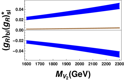
(a)

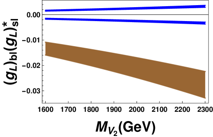
(b)

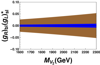
(c)

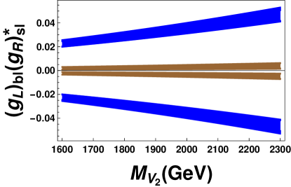
(d)

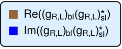
(e)

Figure 1: The constraints on the parameter spaces of the $V_{2}$ VLQ model due to the experimental values provided in introduction. The vertical axes for the plots are products of the model-couplings. In a clockwise fashion, they are: (a)$(g_{R})_{b\ell}(g_{R})_{s\ell}^{*}$ , (b)$(g_{L})_{b\ell}(g_{L})_{s\ell}^{*}$ , (c)$(g_{R})_{b\ell}(g_{L})_{s\ell}^{*}$ and (d)$(g_{L})_{b\ell}(g_{R})_{s\ell}^{*}$. The horizontal axis represents the mass of the $V_{2}$ VLQ in GeV for all four cases. The range for the same is in accordance with the limits obtained from the collider analysis provided in the next section. The brown bands correspond to the real and the blue bands correspond to the imaginary parts of the corresponding coupling products depicted along the vertical axis of each plot. The legend is provided at the bottom. In the above, $\ell=\mu$.

Fig. 1(a) displays the variation of the real and imaginary parts of the coupling product $(g_{R})_{b\ell}(g_{R})_{s\ell}^{*}$ with respect to the mass of the $V_{2}$ LQ $M_{V_{2}}$. The variation for the real (imaginary) part is due to the real (imaginary) part of the solution for the WC $C_{9}$ with respect to the experimental observables given in introduction. The real part of $C_{9}$ has a unique solution, resulting in the single brown band close to the horizontal axis in fig. 1(a). However, the imaginary part of $C_{9}$ has two sets of solutions which are symmetric with respect to 0, and hence translate into the blue bands symmetric with respect to to the horizontal axis. Similarly, the real and imaginary parts for the $C_{10}^{\prime}$ WC translate into fig. 1(b). The unique negative solution for the real part translates into the wide brown band and the solutions for the imaginary part give rise to the blue bands symmetric to the horizontal axis for the coupling product $(g_{L})_{b\ell}(g_{L})_{s\ell}^{*}$. For a benchmark value $M_{V_{2}}=1600$ GeV, the ranges for the real and imaginary parts of these coupling products are:

$${\rm Re}((g_{R})_{b\ell}(g_{R})_{s\ell}^{*}) \in [0.0019,0.0023],$$

$$~{}{\rm Im}((g_{R})_{b\ell}(g_{R})_{s\ell}^{*}) \in \big{(}[0.020,0.025],[-0.025,-0.020]\big{)};$$

$${\rm Re}((g_{L})_{b\ell}(g_{L})_{s\ell}^{*}) \in [-0.016,-0.011],$$

$$~{}{\rm Im}((g_{L})_{b\ell}(g_{L})_{s\ell}^{*}) \in \big{(}[0.0014,0.0018],[-0.0018,-0.0014]\big{)}.$$

The cases 1(c) and 1(d) are a little different from the cases discussed above. 1(c) arises due to $C_{P}$, both of whose real and imaginary part have two solutions, one positive and one negative, at both the higher and lower limits considering experimental errors. However, the regions for these solutions overlap, and hence get broad brown and blue bands both above and below the horizontal axis for each of the real and imaginary parts of the coupling product $(g_{R})_{b\ell}(g_{L})_{s\ell}^{*}$. Similarly, the different sets of solutions for the $C_{S}^{\prime}$ WC translate into fig. 1(d) for the coupling product $(g_{L})_{b\ell}(g_{R})_{s\ell}^{*}$. These solutions do not overlap as in the case of 1(c), and hence we get distinct bands corresponding to the real and imaginary parts of the corresponding coupling product. As in the former cases, we provide values for these coupling products for the benchmark value $M_{V_{2}}=1600$ GeV:

$${\rm Re}((g_{R})_{b\ell}(g_{L})_{s\ell}^{*}) \in [-0.025,0.025],$$

$$~{}{\rm Im}((g_{R})_{b\ell}(g_{L})_{s\ell}^{*}) \in [-0.0032,0.0032];$$

$${\rm Re}((g_{L})_{b\ell}(g_{R})_{s\ell}^{*}) \in \big{(}[-0.0035,-0.0014],[0.0006,0.003]\big{)},$$

$${\rm Im}((g_{L})_{b\ell}(g_{R})_{s\ell}^{*}) \in \big{(}[-0.025,-0.020],[0.020,0.025]\big{)}.$$

4 Collider Analysis

In this section we study the collider prospects of $V_{2}$ VLQ at the LHC. We look for signals where the $V_{2}$ VLQ decays into a bottom quark ($b$) and a lepton ($\ell\equiv e,\mu$) with a branching ratio that depends on the corresponding coupling. We vary the coupling of $V_{2}$ to $b$ quark and $\ell$ from 0.1 to 0.9. As a result, the branching ratio varies from $11\%$ to $47.9\%$ for individual light leptonic channels. For further simplicity, we assume the coupling of $V_{2}$ to both lepton and bottom quark to be equal while that to the rest of the quarks and leptons is fixed at 0.1. Hence, the signal we consider from VLQ pair production is two $b$-jets with $P_{T}^{b-{\rm jet}}\geq 20$ GeV and $|\eta_{b-{\rm jet}}|\leq 2.4$ and two light leptons with $P_{T}^{\ell}\geq 10$ GeV and $|\eta_{\ell}|\leq 2.4$. The dominant backgrounds from the SM processes are $t\bar{t}$ + jets, $t\bar{t}W^{\pm}$+ jets and $t\bar{t}Z$+ jets. Furthermore, the SM process which contribute sub-dominantly are $tW^{\pm}$ + jets and $ZZ$ + jets. The SM processes like $W^{+}W^{-}$ + jets, $ZW^{\pm}$ + jets, $Z$+ jets and $W^{\pm}$+ jets contribute mildly to this analysis because we tag two $b$-jets in the final states. We therefore do not consider these backgrounds in our present analysis.

Both the signal and SM background processes in this analysis have been generated using Madgraph5 [93] with the default parton distribution functions NNPDF3.0 [94]. The VLQ model file used in this analysis is obtained from FeynRules [81]. The parton level events generated from Madgraph5 are then passed through Pythia8 [95] for showering and hadronization. The backgrounds and signal events are matched properly using the MLM matching scheme [96]. The detector level simulation is done using Delphes(v3) [97] and the jets are constructed using fastjet [98] with anti-$K_{T}$ jet algorithm with radius $R=0.5$ and $P_{T}>20$ GeV. The cross-section corresponding to the background processes that have been used in this analysis are provided in table 1. The signal cross-section is calculated from Madgraph at LO (leading-order).

Background process	cross-section (pb)
$t\bar{t}$ (NNLO + NNLL)	815.96 [99]
$tW^{\pm}$ (NLO + NNLL)	71.7 [100]
$t\bar{t}W^{\pm}(Z)$ (NLO)	0.6448 (0.8736) [101]
$ZZ$ (NLO)	16.91 [102]

Table 1: The cross-sections for the background processes used in this analysis are shown with the order (of QCD corrections) provided in brackets. For $t\bar{t}$, this is calculated using the Top++2.0 program up to NNLO in perturbative QCD and soft-gluon resummation up to NNLL order with the assumption that the top quark mass is 173.2 GeV.

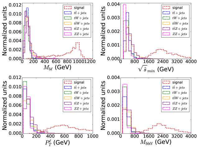
Figure 2: Kinematic variables which efficiently discriminate between signal and background events are displayed here. The signal is represented by red dashed line where the $V_{2}$ mass is considered to be 1 TeV.

We have utilized some interesting kinematic variables which efficiently discriminate the signal and background events and maximizes the signal reach at the LHC. These variables are $\sqrt{\hat{s}}_{min}$ [103, 104, 105], transverse momentum of the lepton, invariant mass of the $b$-jet and lepton, and the invariant mass of two $b$-jets and the di-lepton. In addition, we also make use of the di-lepton invariant mass to handle the backgrounds involving the $Z$-boson. The kinematic variable $\sqrt{\hat{s}}_{min}$ was originally proposed in order to measure the mass scale of NP produced at the LHC. It is defined as the minimum partonic CM energy that is consistent with the final state measured momenta and the missing transverse energy of the event. Mathematically, this variable is defined as,

$$\sqrt{\hat{s}_{\min}(M_{inv})}=\sqrt{(E^{vis})^{2}-(P_{z}^{vis})^{2}}+\sqrt{\,\not\!\vec{P}_{T}^{2}+M_{inv}^{2}}\;\;,$$ (11)

where $M_{inv}$ is the sum of the masses for the “invisible” particles. $E^{vis}=\sum_{j}e^{vis}_{j}$ is the total energy and $P_{z}^{vis}=\sum_{j}p^{z}_{j}$ the total longitudinal momentum of the “visible” particles. In this analysis we take two $b$-jets and two leptons as our “visible” particles and use their momenta for calculating $\sqrt{\hat{s}}_{min}$. Since the signal we consider here does not involve any invisible particle, the missing energy in each event is very small and can solely be attributed to mis-measurement. $M_{inv}$ is also taken to be zero due to the same reason. As per our expectations, $\sqrt{\hat{s}}_{min}$ peaks at twice the mass of the LQ as shown by the red dashed distribution in fig. 2 (top panel right plot). The VLQ mass, for this representative plot, is taken to be 1 TeV.

Similarly, the other variables like the invariant mass of the two $b$-jets and the two leptons ($M_{bb\ell\ell}$), and of one $b$-jet and corresponding lepton ($M_{b\ell}$) are also very efficient in separating the signal from the backgrounds. While the invariant mass $M_{bb\ell\ell}$ peaks at the at twice the mass of the VLQ, the variable $M_{b\ell}$ peaks at mass of the VLQ (1 TeV) as expected. Since the lepton from the VLQ is highly boosted, we also have utilized the lepton transverse momenta, $P_{T}^{\ell}$, as a discriminating variable.

With the above variables we have done a cut based analysis where the following cuts are employed to maximize the signal significance,

• $\sqrt{\hat{s}}_{min}>1600$ GeV,

• $P_{T}^{\ell}>150$ GeV,

• $M_{b\ell}>150$ GeV,

• $M_{bb\ell\ell}>1450$ GeV,

• $M_{\ell\ell}>110$ GeV.

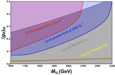
Figure 3: The $2\sigma$ exclusion limits for the 13 TeV CM energy are displayed for the signal with integrated luminosities of 300 $\rm{fb}^{-1}$ (red band) and 3000 $\rm{fb}^{-1}$ (blue band) respectively. The grey band represents the constraints from the flavour physics WC $C_{P}$ which contribute to the $b\to s\ell^{+}\ell^{-}$ transition as shown in eq. 10. The yellow band represents constraints due to the same sub-quark process coming from the $\Delta C_{9}$ WC.

After implementing the above cuts, we have calculated the signal significance using the following formula,

$${\cal S}=\sqrt{2\times[(N_{S}+N_{B})~{}{\rm ln}(1+\frac{N_{S}}{N_{B}})-N_{S}]}.$$ (12)

Here $N_{S}(N_{B})$ represent the number of signal (background) events for a given luminosity after implementing the cuts mentioned above. Eq. 12 allows us to exclude the mass of the $V_{2}$ VLQ up to 2140 GeV for the coupling $(g_{R})_{b\ell}=0.9$ at $95\%$ C.L. for 13 TeV LHC with 300 $\rm{fb}^{-1}$ of integrated luminosity. This limit is reduced to a value as low as 1.6 TeV for $(g_{R})_{b\ell}=0.1$ (displayed in fig. 3 with red band) at $95\%$ C.L. for 300 $\rm{fb}^{-1}$ of integrated luminosity. As is evident from the figure, the exclusion limit can go up to 2340 GeV for 3000 $\rm{fb}^{-1}$ at $95\%$ C.L. for $(g_{R})_{b\ell}=0.9$ and for $(g_{R})_{b\ell}=0.1$ the limit is 1.8 TeV which is represented by the blue band. Note that one might expect a better limit by limiting the other coupling(s) to a very small value (which, as mentioned earlier we have taken to be 0.1) so that the considered channel will get $100\%$ branching ratio. However, that limit as we have checked, is marginally better than for $(g_{R})_{b\ell}=0.9$ because even in this case also the branching ratio approaches $100\%$. Hence, in this analysis, the limits that we have obtained for $V_{2}$ VLQ in mass and coupling plane from the collider study in conjunction with the flavour physics constraints are more or less optimal.

As discussed earlier in sec. 3 using the WCs of the flavour physics observables like $R_{K}$, $R^{\rm low-bin}_{K^{*}}$, $R^{\rm central-bin}_{K^{*}}$ and ${\rm BR}(B_{s}\to\mu^{+}\mu^{-})$ one can obtain constraints in the VLQ mass and coupling product plane which is demonstrated in fig. 3 by the gray region. The coupling ($(g_{R})_{b\ell}$) represented by the vertical axis is obtained by setting $(g_{R,L})_{s\ell}=0.1$ in the corresponding coupling product. It is however not possible for us to put constraints on the imaginary part of individual couplings from a combined collider and flavour point of view, since the collider analysis inherently assumes the couplings to be real. We find that part of the allowed parameter space for the real part of the coupling $(g_{R})_{b\ell}$ (corresponding to a value of $(g_{R,L})_{s\ell}=0.1$) is disallowed by the collider constraints. However, the parameter space due to flavour constraints from $\Delta C_{9}$ (NP contribution to the WC $C_{9}$) is retained completely. We hence conclude that the values for $(g_{R})_{b\ell}$ that fall within the yellow band in fig. 3 represent the allowed parameter space upto $1\sigma$ with respect to the mass of the $V_{2}$ VLQ for all collider and flavour constraints taken together. At this point we remark in passing that, a similar analysis can also be done for $(g_{L})_{b\ell}$. However, from fig. 1 it is clear that one will not obtain common points for the real part of such a coupling after requiring $(g_{R,L})_{s\ell}=0.1$ from the flavour analysis alone (see figs. 1b and 1d). Moreover, most of the allowed parameter space for such a scenario will correspond to negative values of $(g_{L})_{b\ell}$ and hence will have no intersection with the constraints due to the collider analysis. This will hence provide no further insight as to the allowed parameter space for such a coupling and hence we refrain from showing the corresponding plot.

5 Conclusion

We consider a component ($V^{\frac{4}{3}}_{2}\equiv V_{2}$) of the ${V_{2}}$ VLQ of electromagnetic charge $\frac{4}{3}$ which mediates $b\to s$ neutral current processes at tree level. We use the $R_{K}$, $R^{\rm low-bin}_{K^{*}}$, $R^{\rm central-bin}_{K^{*}}$ and ${\rm BR}(B_{s}\to\mu^{+}\mu^{-})$ data along with their $1\sigma$ errors in order to numerically solve for the involved Wilson coefficients, and, in turn, provide constraints on the product of coupling with respect to the mass of the $V_{2}$ VLQ. Simultaneously, we probe this VLQ at 13 TeV LHC via $b\bar{b}\ell^{+}\ell^{-}$ final state. For a reliable collider analysis we have accounted for several relevant SM background processes. Using different interesting kinematic variables and with judicious cut selections we maximise the signal significance with respect to the SM backgrounds. Our collider study reveals that it is possible to maximally exclude the mass of the $V_{2}$ VLQ up to 2340 GeV at 95% C.L. at the 13 TeV LHC for an integrated luminosity of 3000 ${\rm fb}^{-1}$. In addition, our collier study reduces chunk of parameter space that is consistent with the $b\to s$ neutral current observables in the $(g_{R})_{b\ell}$ coupling and VLQ mass plane for a fixed value of $(g_{R,L})_{s\ell}=0.1$.

Acknowledgements AS would like to thank Ilja Dorsner for discussions regarding the implementation of the model file for ${V_{2}}$ leptoquark in FeynRules. AKS acknowledges the support received from Department of Science and Technology, Government of India under the fellowship reference number PDF/2017/002935 (SERB NPDF).

References

- [1] CMS collaboration, S. Chatrchyan et al., Observation of a new boson at a mass of 125 GeV with the CMS experiment at the LHC, Phys. Lett. B716 (2012) 30–61, [1207.7235].
- [2] ATLAS collaboration, G. Aad et al., Observation of a new particle in the search for the Standard Model Higgs boson with the ATLAS detector at the LHC, Phys. Lett. B716 (2012) 1–29, [1207.7214].
- [3] HFAG, “Average of and for FPCP 2017.” http://www.slac.stanford.edu/xorg/hflav/semi/fpcp17/RDRDs.html.
- [4] LHCb collaboration, R. Aaij et al., Measurement of the ratio of branching fractions /, Phys. Rev. Lett. 120 (2018) 121801, [1711.05623].
- [5] LHCb collaboration, R. Aaij et al., Test of lepton universality using decays, Phys. Rev. Lett. 113 (2014) 151601, [1406.6482].
- [6] S. Descotes-Genon, L. Hofer, J. Matias and J. Virto, Global analysis of anomalies, JHEP 06 (2016) 092, [1510.04239].
- [7] M. Bordone, G. Isidori and A. Pattori, On the Standard Model predictions for and , Eur. Phys. J. C76 (2016) 440, [1605.07633].
- [8] LHCb collaboration, R. Aaij et al., Test of lepton universality with decays, JHEP 08 (2017) 055, [1705.05802].
- [9] B. Capdevila, A. Crivellin, S. Descotes-Genon, J. Matias and J. Virto, Patterns of New Physics in transitions in the light of recent data, JHEP 01 (2018) 093, [1704.05340].
- [10] B. Schrempp and F. Schrempp, LIGHT LEPTOQUARKS, Phys. Lett. 153B (1985) 101–107.
- [11] H. Georgi and S. L. Glashow, Unity of All Elementary Particle Forces, Phys. Rev. Lett. 32 (1974) 438–441.
- [12] J. C. Pati and A. Salam, Is Baryon Number Conserved?, Phys. Rev. Lett. 31 (1973) 661–664.
- [13] S. Dimopoulos and L. Susskind, Mass Without Scalars, Nucl. Phys. B155 (1979) 237–252.
- [14] S. Dimopoulos, Technicolored Signatures, Nucl. Phys. B168 (1980) 69–92.
- [15] P. Langacker, Grand Unified Theories and Proton Decay, Phys. Rept. 72 (1981) 185.
- [16] G. Senjanovic and A. Sokorac, Light Leptoquarks in SO(10), Z. Phys. C20 (1983) 255.
- [17] R. J. Cashmore et al., EXOTIC PHENOMENA IN HIGH-ENERGY E P COLLISIONS, Phys. Rept. 122 (1985) 275–386.
- [18] J. C. Pati and A. Salam, Lepton Number as the Fourth Color, Phys. Rev. D10 (1974) 275–289.
- [19] M. B. Green and J. H. Schwarz, Anomaly Cancellation in Supersymmetric D=10 Gauge Theory and Superstring Theory, Phys. Lett. 149B (1984) 117–122.
- [20] E. Witten, Symmetry Breaking Patterns in Superstring Models, Nucl. Phys. B258 (1985) 75.
- [21] D. J. Gross, J. A. Harvey, E. J. Martinec and R. Rohm, The Heterotic String, Phys. Rev. Lett. 54 (1985) 502–505.
- [22] J. L. Hewett and T. G. Rizzo, Low-Energy Phenomenology of Superstring Inspired E(6) Models, Phys. Rept. 183 (1989) 193.
- [23] S. Davidson, D. C. Bailey and B. A. Campbell, Model independent constraints on leptoquarks from rare processes, Z. Phys. C61 (1994) 613–644, [hep-ph/9309310].
- [24] J. L. Hewett and T. G. Rizzo, Much ado about leptoquarks: A Comprehensive analysis, Phys. Rev. D56 (1997) 5709–5724, [hep-ph/9703337].
- [25] P. Nath and P. Fileviez Perez, Proton stability in grand unified theories, in strings and in branes, Phys. Rept. 441 (2007) 191–317, [hep-ph/0601023].
- [26] O. U. Shanker, Flavor Violation, Scalar Particles and Leptoquarks, Nucl. Phys. B206 (1982) 253–272.
- [27] O. U. Shanker, 2, 3 and 0 Constraints on Leptoquarks and Supersymmetric Particles, Nucl. Phys. B204 (1982) 375–386.
- [28] W. Buchmuller and D. Wyler, Constraints on SU(5) Type Leptoquarks, Phys. Lett. B177 (1986) 377–382.
- [29] W. Buchmuller, R. Ruckl and D. Wyler, Leptoquarks in Lepton - Quark Collisions, Phys. Lett. B191 (1987) 442–448.
- [30] J. L. Hewett and S. Pakvasa, Leptoquark Production in Hadron Colliders, Phys. Rev. D37 (1988) 3165.
- [31] M. Leurer, A Comprehensive study of leptoquark bounds, Phys. Rev. D49 (1994) 333–342, [hep-ph/9309266].
- [32] M. Leurer, Bounds on vector leptoquarks, Phys. Rev. D50 (1994) 536–541, [hep-ph/9312341].
- [33] CDF collaboration, T. Aaltonen et al., Search for Third Generation Vector Leptoquarks in Collisions at = 1.96-TeV, Phys. Rev. D77 (2008) 091105, [0706.2832].
- [34] I. Dorsner, S. Fajfer and A. Greljo, Cornering Scalar Leptoquarks at LHC, JHEP 10 (2014) 154, [1406.4831].
- [35] B. Allanach, A. Alves, F. S. Queiroz, K. Sinha and A. Strumia, Interpreting the CMS Excess with a Leptoquark Model, Phys. Rev. D92 (2015) 055023, [1501.03494].
- [36] J. L. Evans and N. Nagata, Signatures of Leptoquarks at the LHC and Right-handed Neutrinos, Phys. Rev. D92 (2015) 015022, [1505.00513].
- [37] X.-Q. Li, Y.-D. Yang and X. Zhang, Revisiting the one leptoquark solution to the R(D(∗)) anomalies and its phenomenological implications, JHEP 08 (2016) 054, [1605.09308].
- [38] B. Diaz, M. Schmaltz and Y.-M. Zhong, The leptoquark Hunter’s guide: Pair production, JHEP 10 (2017) 097, [1706.05033].
- [39] B. Dumont, K. Nishiwaki and R. Watanabe, LHC constraints and prospects for scalar leptoquark explaining the anomaly, Phys. Rev. D94 (2016) 034001, [1603.05248].
- [40] D. A. Faroughy, A. Greljo and J. F. Kamenik, Confronting lepton flavor universality violation in B decays with high- tau lepton searches at LHC, Phys. Lett. B764 (2017) 126–134, [1609.07138].
- [41] A. Greljo and D. Marzocca, High- dilepton tails and flavor physics, Eur. Phys. J. C77 (2017) 548, [1704.09015].
- [42] CMS collaboration, D. Baumgartel, Searches for the pair production of scalar leptoquarks at CMS, J. Phys. Conf. Ser. 485 (2014) 012053.
- [43] ATLAS collaboration, G. Aad et al., Searches for scalar leptoquarks in pp collisions at = 8 TeV with the ATLAS detector, Eur. Phys. J. C76 (2016) 5, [1508.04735].
- [44] ATLAS collaboration, M. Aaboud et al., Search for scalar leptoquarks in pp collisions at = 13 TeV with the ATLAS experiment, New J. Phys. 18 (2016) 093016, [1605.06035].
- [45] CMS collaboration, A. M. Sirunyan et al., Search for third-generation scalar leptoquarks and heavy right-handed neutrinos in final states with two tau leptons and two jets in proton-proton collisions at TeV, JHEP 07 (2017) 121, [1703.03995].
- [46] CMS collaboration, A. M. Sirunyan et al., Search for third-generation scalar leptoquarks decaying to a top quark and a lepton at 13 TeV, Eur. Phys. J. C78 (2018) 707, [1803.02864].
- [47] I. Doršner, S. Fajfer, D. A. Faroughy and N. Košnik, The role of the GUT leptoquark in flavor universality and collider searches, 1706.07779.
- [48] B. C. Allanach, B. Gripaios and T. You, The case for future hadron colliders from decays, JHEP 03 (2018) 021, [1710.06363].
- [49] A. Crivellin, D. Müller and T. Ota, Simultaneous explanation of R(D(∗)) and b→sμ+ μ−: the last scalar leptoquarks standing, JHEP 09 (2017) 040, [1703.09226].
- [50] G. Hiller and I. Nisandzic, and beyond the standard model, Phys. Rev. D96 (2017) 035003, [1704.05444].
- [51] D. Buttazzo, A. Greljo, G. Isidori and D. Marzocca, B-physics anomalies: a guide to combined explanations, JHEP 11 (2017) 044, [1706.07808].
- [52] L. Calibbi, A. Crivellin and T. Li, A model of vector leptoquarks in view of the -physics anomalies, 1709.00692.
- [53] S. Sahoo, R. Mohanta and A. K. Giri, Explaining the and anomalies with vector leptoquarks, Phys. Rev. D95 (2017) 035027, [1609.04367].
- [54] W. Altmannshofer, P. Bhupal Dev and A. Soni, anomaly: A possible hint for natural supersymmetry with -parity violation, Phys. Rev. D96 (2017) 095010, [1704.06659].
- [55] A. Biswas, D. Kumar Ghosh, N. Ghosh, A. Shaw and A. K. Swain, Novel collider signature of Leptoquark and observables, 1808.04169.
- [56] M. Blanke and A. Crivellin, Meson Anomalies in a Pati-Salam Model within the Randall-Sundrum Background, Phys. Rev. Lett. 121 (2018) 011801, [1801.07256].
- [57] Y. Sakaki, M. Tanaka, A. Tayduganov and R. Watanabe, Testing leptoquark models in , Phys. Rev. D88 (2013) 094012, [1309.0301].
- [58] D. Bečirević, S. Fajfer, N. Košnik and O. Sumensari, Leptoquark model to explain the -physics anomalies, and , Phys. Rev. D94 (2016) 115021, [1608.08501].
- [59] O. Popov and G. A. White, One Leptoquark to unify them? Neutrino masses and unification in the light of , and anomalies, Nucl. Phys. B923 (2017) 324–338, [1611.04566].
- [60] C.-H. Chen, T. Nomura and H. Okada, Excesses of muon , , and in a leptoquark model, Phys. Lett. B774 (2017) 456–464, [1703.03251].
- [61] D. Bečirević and O. Sumensari, A leptoquark model to accommodate and , JHEP 08 (2017) 104, [1704.05835].
- [62] A. K. Alok, B. Bhattacharya, A. Datta, D. Kumar, J. Kumar and D. London, New Physics in after the Measurement of , Phys. Rev. D96 (2017) 095009, [1704.07397].
- [63] N. Assad, B. Fornal and B. Grinstein, Baryon Number and Lepton Universality Violation in Leptoquark and Diquark Models, Phys. Lett. B777 (2018) 324–331, [1708.06350].
- [64] D. Aloni, A. Dery, C. Frugiuele and Y. Nir, Testing minimal flavor violation in leptoquark models of the anomaly, JHEP 11 (2017) 109, [1708.06161].
- [65] I. G. B. Wold, S. L. Finkelstein, A. J. Barger, L. L. Cowie and B. Rosenwasser, A Faint Flux-Limited Lyman Alpha Emitter Sample at , Astrophys. J. 848 (2017) 108, [1709.06092].
- [66] D. Müller, Leptoquarks in Flavour Physics, EPJ Web Conf. 179 (2018) 01015, [1801.03380].
- [67] G. Hiller, D. Loose and I. Nišandžić, Flavorful leptoquarks at hadron colliders, Phys. Rev. D97 (2018) 075004, [1801.09399].
- [68] A. Biswas, D. K. Ghosh, A. Shaw and S. K. Patra, anomalies in light of extended scalar sectors, 1801.03375.
- [69] S. Fajfer, N. Košnik and L. Vale Silva, Footprints of leptoquarks: from to , Eur. Phys. J. C78 (2018) 275, [1802.00786].
- [70] A. Monteux and A. Rajaraman, B Anomalies and Leptoquarks at the LHC: Beyond the Lepton-Quark Final State, 1803.05962.
- [71] D. Bečirević, B. Panes, O. Sumensari and R. Zukanovich Funchal, Seeking leptoquarks in IceCube, JHEP 06 (2018) 032, [1803.10112].
- [72] J. Kumar, D. London and R. Watanabe, Combined Explanations of the and Anomalies: a General Model Analysis, 1806.07403.
- [73] A. Crivellin, C. Greub, F. Saturnino and D. Müller, Importance of Loop Effects in Explaining the Accumulated Evidence for New Physics in B Decays with a Vector Leptoquark, 1807.02068.
- [74] A. Angelescu, D. Bečirević, D. A. Faroughy and O. Sumensari, Closing the window on single leptoquark solutions to the -physics anomalies, JHEP 10 (2018) 183, [1808.08179].
- [75] LHCb, CMS collaboration, V. Khachatryan et al., Observation of the rare decay from the combined analysis of CMS and LHCb data, Nature 522 (2015) 68–72, [1411.4413].
- [76] C. Bobeth, M. Gorbahn, T. Hermann, M. Misiak, E. Stamou and M. Steinhauser, in the Standard Model with Reduced Theoretical Uncertainty, Phys. Rev. Lett. 112 (2014) 101801, [1311.0903].
- [77] P. Bandyopadhyay and R. Mandal, Revisiting scalar leptoquark at the LHC, Eur. Phys. J. C78 (2018) 491, [1801.04253].
- [78] N. Vignaroli, Seeking LQs in the plus missing energy channel at the high-luminosity LHC, 1808.10309.
- [79] I. Doršner and A. Greljo, Leptoquark toolbox for precision collider studies, JHEP 05 (2018) 126, [1801.07641].
- [80] CMS collaboration, A. M. Sirunyan et al., Search for leptoquarks coupled to third-generation quarks in proton-proton collisions at 13 TeV, Submitted to: Phys. Rev. Lett. (2018) , [1809.05558].
- [81] A. Alloul, N. D. Christensen, C. Degrande, C. Duhr and B. Fuks, FeynRules 2.0 - A complete toolbox for tree-level phenomenology, Comput. Phys. Commun. 185 (2014) 2250–2300, [1310.1921].
- [82] ATLAS collaboration, T. A. collaboration, A search for B-L R-parity-violating scalar tops in = 13 TeV collisions with the ATLAS experiment, .
- [83] I. Doršner, S. Fajfer, A. Greljo, J. F. Kamenik and N. Košnik, Physics of leptoquarks in precision experiments and at particle colliders, Phys. Rept. 641 (2016) 1–68, [1603.04993].
- [84] N. Kosnik, Model independent constraints on leptoquarks from processes, Phys. Rev. D86 (2012) 055004, [1206.2970].
- [85] B. Grinstein, M. J. Savage and M. B. Wise, in the Six Quark Model, Nucl. Phys. B319 (1989) 271–290.
- [86] C. Bobeth, M. Misiak and J. Urban, Photonic penguins at two loops and dependence of , Nucl. Phys. B574 (2000) 291–330, [hep-ph/9910220].
- [87] A. J. Buras, M. Misiak, M. Munz and S. Pokorski, Theoretical uncertainties and phenomenological aspects of decay, Nucl. Phys. B424 (1994) 374–398, [hep-ph/9311345].
- [88] C. Bobeth, G. Hiller and G. Piranishvili, Angular distributions of decays, JHEP 12 (2007) 040, [0709.4174].
- [89] W. Altmannshofer and D. M. Straub, New physics in transitions after LHC run 1, Eur. Phys. J. C75 (2015) 382, [1411.3161].
- [90] HPQCD collaboration, C. Bouchard, G. P. Lepage, C. Monahan, H. Na and J. Shigemitsu, Rare decay form factors from lattice QCD, Phys. Rev. D88 (2013) 054509, [1306.2384].
- [91] P. Ball and R. Zwicky, New results on decay formfactors from light-cone sum rules, Phys. Rev. D71 (2005) 014015, [hep-ph/0406232].
- [92] M. Bartsch, M. Beylich, G. Buchalla and D. N. Gao, Precision Flavour Physics with and , JHEP 11 (2009) 011, [0909.1512].
- [93] J. Alwall, R. Frederix, S. Frixione, V. Hirschi, F. Maltoni, O. Mattelaer et al., The automated computation of tree-level and next-to-leading order differential cross sections, and their matching to parton shower simulations, JHEP 07 (2014) 079, [1405.0301].
- [94] NNPDF collaboration, R. D. Ball et al., Parton distributions for the LHC Run II, JHEP 04 (2015) 040, [1410.8849].
- [95] T. Sjöstrand, S. Ask, J. R. Christiansen, R. Corke, N. Desai, P. Ilten et al., An Introduction to PYTHIA 8.2, Comput. Phys. Commun. 191 (2015) 159–177, [1410.3012].
- [96] S. Hoeche, F. Krauss, N. Lavesson, L. Lonnblad, M. Mangano, A. Schalicke et al., Matching parton showers and matrix elements, in HERA and the LHC: A Workshop on the implications of HERA for LHC physics: Proceedings Part A, pp. 288–289, 2005, hep-ph/0602031, DOI.
- [97] DELPHES 3 collaboration, J. de Favereau, C. Delaere, P. Demin, A. Giammanco, V. Lemaître, A. Mertens et al., DELPHES 3, A modular framework for fast simulation of a generic collider experiment, JHEP 02 (2014) 057, [1307.6346].
- [98] M. Cacciari, G. P. Salam and G. Soyez, FastJet User Manual, Eur. Phys. J. C72 (2012) 1896, [1111.6097].
- [99] M. Czakon and A. Mitov, Top++: A Program for the Calculation of the Top-Pair Cross-Section at Hadron Colliders, Comput. Phys. Commun. 185 (2014) 2930, [1112.5675].
- [100] N. Kidonakis, Theoretical results for electroweak-boson and single-top production, PoS DIS2015 (2015) 170, [1506.04072].
- [101] F. Maltoni, D. Pagani and I. Tsinikos, Associated production of a top-quark pair with vector bosons at NLO in QCD: impact on searches at the LHC, JHEP 02 (2016) 113, [1507.05640].
- [102] F. Cascioli, T. Gehrmann, M. Grazzini, S. Kallweit, P. Maierhöfer, A. von Manteuffel et al., ZZ production at hadron colliders in NNLO QCD, Phys. Lett. B735 (2014) 311–313, [1405.2219].
- [103] P. Konar, K. Kong and K. T. Matchev, : A Global inclusive variable for determining the mass scale of new physics in events with missing energy at hadron colliders, JHEP 03 (2009) 085, [0812.1042].
- [104] P. Konar, K. Kong, K. T. Matchev and M. Park, RECO level and subsystem : Improved global inclusive variables for measuring the new physics mass scale in events at hadron colliders, JHEP 06 (2011) 041, [1006.0653].
- [105] A. K. Swain and P. Konar, Constrained and reconstructing with semi-invisible production at hadron colliders, JHEP 03 (2015) 142, [1412.6624].